Metastability versus collapse following a quench in attractive Bose-Einstein condensates

Abstract

We consider a Bose-Einstein condensate (BEC) with attractive two-body interactions in a cigar-shaped trap, initially prepared in its ground state for a given negative scattering length, which is quenched to a larger absolute value of the scattering length. Using the mean-field approximation, we compute numerically, for an experimentally relevant range of aspect ratios and initial strengths of the coupling, two critical values of quench: one corresponds to the weakest attraction strength the quench to which causes the system to collapse before completing even a single return from the narrow configuration (“pericenter”) in its breathing cycle. The other is a similar critical point for the occurrence of collapse before completing two returns. In the latter case, we also compute the limiting value, as we keep increasing the strength of the post-quench attraction towards its critical value, of the time interval between the first two pericenters. We also use a Gaussian variational model to estimate the critical quenched attraction strength below which the system is stable against the collapse for long times. These time intervals and critical attraction strengths—apart from being fundamental properties of nonlinear dynamics of self-attractive BECs—may provide clues to the design of upcoming experiments that are trying to create robust BEC breathers.

I Introduction

Presently, at least two experimental groups Everitt et al. (2015); Hulet (2016) are trying to realize Gross-Pitaevskii breathers Zakharov and Shabat (1972); Satsuma and Yajima (1974); Sakaguchi and Malomed (2004); Prilepsky and Derevyanko (2007); Yanay et al. (2009); Dunjko and Olshanii (2015) in attractive Bose-Einstein condensates (BECs) Pethick and Smith (2008). Their immediate goal is to create conditions such that the system is well-described by the one-dimensional (1D) integrable nonlinear Schrödinger equation (NLSE),

$$i\psi_{t}=-\frac{1}{2}\psi_{xx}+\eta\left|\psi\right|^{2}\psi$$ (1)

Ablowitz and Segur (1981), with $\eta<0$, and then to excite a breather—a “nonlinear superposition” of fundamental NLSE solitons whose centers of mass coincide and which are at rest relative to each other Cardoso et al. (2010). Experimentally, the effectively 1D approximation is provided by placing the BEC in a elongated, cigar-shaped trap Castin (2004). The breather that is the principal target of the current experimental efforts is shown in Fig. 1. Apart from being objects of interest in their own right, breathers are also potentially useful in atomic interferometry Dunjko and Olshanii (2015).

Figure 1: The $\mathbf{1\,\mathord{:}\,3}$ breather. The density profile, at three points of time, of an exact two-soliton solution of the integrable 1D NLSE, built of fundamental solitons with coinciding centers, zero velocities, and norms $1/4$ and $3/4$. The solid line corresponds to the initial profile, the dotted line to the profile at $1/4$ density period, and the dashed line to $1/2$ period.

Breathers may be excited by quenching the nonlinearity strength $\eta$ in Eq. (1). Here and below, by the “strength” of a negative quantity we mean its magnitude, and, accordingly, by “stronger” and “weaker” we will mean interaction strengths which are larger and smaller in magnitude, respectively. In BECs, the quench can be applied via magnetically tuned Feshbach resonances Chin et al. (2010); Nguyen et al. (2014). Here one may take advantage of a special property of the integrable NLSE: Consider an $N$-soliton breather, composed of $N$ fundamental solitons with norm ratios $1\,\mathord{:}\,3\,\mathord{:}\,5\,\mathord{:}\,7\,\mathord{:}\,\ldots\,\,\mathord{:}\,(2N-1)$ (an “odd-norm-ratio breather”), with their phases synchronized initially. At the point in its breathing cycle at which it is the widest (the “apocenter”), its wave function is the same as for a fundamental soliton generated by Eq. (1) with the value of $\eta$ which is smaller by a factor of $N^{2}$ Satsuma and Yajima (1974). Thus, for example, to excite the $1\,\mathord{:}\,3$ breather, we first prepare a fundamental soliton of the NLSE, and then apply the quench, suddenly multiplying $\eta$ by $4$.

Following the quench, the system will start to “breathe,” alternating between a narrow density profile (the “pericenter”) and a wide one (the “apocenter”). For the quench factor close to $4$, numerical simulations produce breathings of the longitudinal density profile which resemble the picture generated by the exact two-soliton solution displayed in Fig. 1, which includes the development, at the pericenter, of the two “dwarf satellite peaks” adjacent to the central peak. Note that the satellite peaks are an interference effect, and do not imply fragmentation of the matter wave. Generally, this picture is quantitatively correct when (1) the 1D approximation is accurate enough, for which we need the effective coupling strength—the product of the absolute value of the scattering length and of the number of particles—to be as small as possible; (2) there is no longitudinal confinement; and (3) the quench factor is close to $4$. For smaller quenches, the satellite peaks do not emerge, while the profile (qualitatively speaking) oscillates between the solid-line and the dotted-line shapes in Fig. 1. On the other hand, for much larger quenches, the breathings become more complex. In particular, if the quench is close to $n^{2}$, with integer $n$, the breathings resemble the well-known exact solutions for $n$-solitons Satsuma and Yajima (1974). For example, the three-dimensional (3D) breathings displayed in Fig. 2 are similar to those of the integrable 1D $3$-soliton with the norm ratio $1\,\mathord{:}\,3\,\mathord{:}\,5$, since the quench is close to 9.

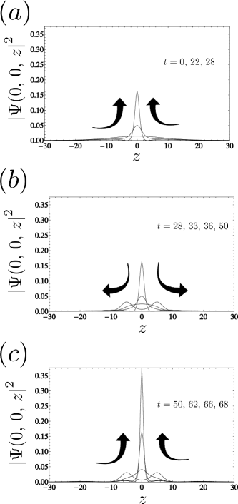
Figure 2: A complex breather. The axial density profile at several points in time of a 3D breather. We are using the “natural units” introduced in the text preceding Eq. (7). The breather is obtained by initializing the system in the ground state of the 3D GPE with $\gamma_{z}=0$ and $\beta=(1/8)\beta_{\text{GS}}$; here $\beta_{\text{GS}}$ is the ground-state critical value of the coupling constant. Then, at $t=0$, we apply the quench factor $9.6$ to produce $\beta=1.2\beta_{\text{GS}}$. Because the quench is close to $3^{2}$, the breathings resemble those of the exact $3$-soliton solution in 1D. Note that the post-quench coupling strength is supercritical, and the variational model of Sec. II suggests that the system eventually collapses. Panel (a) shows the solitary wave initially narrowing until it reaches the “pericenter” at $t=28$. After that, as shown in (b), the system widens until reaching the “apocenter” at $t=50$. The double-peak structure at this moment is a notable feature of the 1D $3$-soliton, although it can also occur for $2$-solitons whose constituent fundamental solitons have comparable norms Dunjko and Olshanii (2015). In panel (c) the system narrows again, until reaching a new, even narrower “pericenter”. Then, the breather begins to widen again (not shown here). Additionally, although it is not well visible on the scale of these plots, following the quench there appears radiation emitted by the breather. Radiation is present in the integrable solution as well, if the quench factor is not exactly the square of an integer Satsuma and Yajima (1974).

Actual experiments deal with 3D settings, even if they correspond to elongated traps. As is well known, 3D self-attractive BECs are unstable against collapse Zakharov and Synakh (1975); Zakharov et al. (1985); Zakharov and Kuznetsov (1986); Sulem and Sulem (1999); Bergé and Rasmussen (2002) whenever the coupling strength exceeds a certain critical value (however, see ). The collapse has been observed and extensively studied experimentally too Gerton et al. (2000); Roberts et al. (2001); Donley et al. (2001); Cornish et al. (2006); Altin et al. (2011); Compton et al. (2012); Eigen et al. (2016). On the theoretical side, a study of direct relevance to the present work was reported in Ref. Gammal et al. (2001). Similar to what we do below, that work also used the mean-field approximation, i.e., the Gross-Pitaevskii equation [GPE, see Eq. (2) below]. It aimed to compute the “ground-state (GS) critical value” (i.e., the value of the coupling strength below which there is a stable GS within the mean-field model, whereas the GS does not exist above the critical value) for the full range of aspect ratios of the cylindrically symmetric trap. For completeness’ sake, we reproduce those results in Table 1 below.

However, breathers are excited states of the system, rather than a GS. Thus, the boundaries of the parameter regime in which the system is stable against dynamical collapse of such states should be re-investigated. To this end, suppose we prepare the BEC in its GS at some sub-critical value of the coupling constant, $\beta_{\text{i}}$ [see Eq. (2) below and the related text for the precise definition of $\beta$], and then quench it to some $\beta_{q}=q\beta_{\text{i}}$, with $q>1$. For every given aspect ratio of the trap and $\beta_{\text{i}}$, there is a critical value of $\beta_{q}$, $\beta_{(\infty)}$, such that the system is stable against collapse at $\left|\beta_{q}\right|<\left|\beta_{(\infty)}\right|$ (at the GPE level) for indefinitely long times, whereas the collapse eventually happens at $\left|\beta_{q}\right|>\left|\beta_{(\infty)}\right|$. Intuitively, one may expect that $\left|\beta_{(\infty)}\right|<\left|\beta_{\text{GS}}\right|$, where $\beta_{\text{GS}}$ is the GS critical value of the coupling. The variational analysis reported in Sec. II turns the intuition into an explicit argument, and provide an estimate for $\beta_{(\infty)}$ (whose absolute value indeed turns out to be bounded by $\left|\beta_{\text{GS}}\right|$, within the variational model). Nevertheless, it is not known, and we do not aim to address this rather complex issue here, whether $\left|\beta_{(\infty)}\right|<\left|\beta_{\text{GS}}\right|$ always holds in the framework of the full GPE.

Note that experimentally relevant time scales cannot be effectively infinite relative to the breathing period Hulet (2016). Thus, it is relevant to consider metastability too.

What we observe numerically is that, in some parameter regions, immediately following the quench, the system keeps shrinking while the height of the central peak increases, leading to an immediate collapse. However, at other values of the parameters, the system completes one or more cycles of sequential narrowing and broadening before it finally collapses, which may be categorized as a delayed collapse Biasi et al. (2017), a kind of metastability. The variational treatment produced in Sec. II offers a qualitative picture for this kind of the metastability.

We should mention that Biasi et al. Biasi et al. (2017) carried out a study very much related to ours, which we discuss in Appendix D. We should also mention the work of Mardonov et al. Mardonov et al. (2015), which studies how one can use spin-orbit coupling to control the collapse of a 2D condensate, even blocking it completely in some regimes.

We will study two kinds of quench-critical coupling strengths, which can be done with reasonable accuracy. One is $\beta_{(1)}$, the smallest (in its absolute value) coupling strength the quench to which causes the system to collapse immediately, before completing even one return from the pericenter. The other, $\beta_{(2)}$, is a critical value for the occurrence of the collapse before completing two returns. In the latter case, we also compute the limiting value, as we keep increasing the coupling strength towards the critical point, of the time interval between the first two pericenters. Here we assume (as corroborated by numerical results) that, as we keep all other parameters fixed, if the system does not collapse before completing a single return from the pericenter for a particular value of the post-quench coupling, it will not collapse either for any smaller value. Conversely, if the system does collapse for a given value of the coupling, it will collapse as well for all larger values. Similar statements hold when considering the collapse before completing two returns. This justifies defining the term “critical” for the above-mentioned special values of the quench factor.

As usual, we start the analysis from the 3D GPE including the harmonic-oscillator trapping potential with transverse and longitudinal frequencies $\omega_{\perp}$ and $\omega_{z}$ Pethick and Smith (2008),

$$i\hbar\partial_{t}\Psi=-\frac{\hbar^{2}}{2m}\nabla^{2}\Psi+gN_{\text{a}}\left|\Psi\right|^{2}\Psi$$

$$+\frac{1}{2}m\left(\omega_{r}^{2}\left(x^{2}+y^{2}\right)+\omega_{z}^{2}z^{2}\right)\Psi\,,$$ (2)

with normalization $\int_{V}\,\left|\Psi(\vec{r},\,t)\right|^{2}\,dV=1$. Here $m$ is the atomic mass, $N_{\text{a}}$ the number of atoms, and $g=4\pi\hbar^{2}a/m$ the coupling constant, $a$ being the scattering length of interatomic interactions. Dimensional analysis shows that the problem has two dimensionless parameters. The usual choice are the following two Gammal et al. (2001): the anisotropy parameter $\gamma_{z}\equiv\omega_{z}/\omega_{r}$, and the parameter $\beta\equiv a_{3D}N_{\textrm{a}}/a_{\perp}$, where $a_{\perp}=\sqrt{\hbar/(m\omega_{r})}$, which compares the strength of the nonlinearity to the strength of the transversal confinement.

For numerical work, it makes sense to use “natural” units, namely those in which $\hbar=m=\omega_{r}=1$ (see Appendix A).

Note that for realistic description of experiments, one would need to include the three-body losses in the model as well as gain from the thermal cloud. But for the purposes of this paper, we will take a more theoretical approach and study the GPE without these terms.

In Table 1, for the sake of completeness we include the tabulated values of $\left|\beta_{\text{GS}}(\gamma_{z})\right|$ from Gammal et al. Gammal et al. (2001).

$\gamma_{z}$	0.01	0.02	0.05	0.1	0.2	0.3	0.5	1.0
$\left|\beta_{\text{GS}}(\gamma_{z})\right|$	0.676	0.676	0.677	0.675	0.666	0.654	0.629	0.575

Table 1: The values of $\left|\beta_{\text{GS}}(\gamma_{z})\right|=(N_{\textrm{a}}\left|a_{3D}\right|)_{\text{crit}}/a_{\perp}$ as a function of the aspect ratio $\gamma_{z}$, for cigar-shaped trapping configurations, as reproduced from Ref. Gammal et al. (2001). In terms of notation adopted in that work, $\gamma_{z}=\lambda$ and $\left|\beta_{\text{GS}}(\gamma_{z})\right|=\lambda^{-1/6}k(\lambda)$.

II The variational model

As the first step of the analysis, we address the problem variationally Anderson et al. (1979); Anderson (1983); Desaix et al. (1989, 1991); Pérez-García et al. (1996). We will be using the following effective equations for matter-wave Gaussian widths ($\mathit{w}_{x}$, $\mathit{w}_{y}$, and $\mathit{w}_{z}$) derived in Ref. Pérez-García et al. (1996); the approach of Ref. Eleftheriou and Huang (2000), although not variational, is similar in spirit. Very similar equations were also used in the study of collapse in Ref. Carr and Castin (2002), except that here it was assumed that the density profile in the $z$-direction is a $\operatorname{sech}$-squared, the shape of the exact 1D single soliton.

$$m\ddot{\mathit{w}}_{x} =\frac{\hbar^{2}}{m\mathit{w}_{x}^{3}}+\frac{gN_{\text{a}}}{(2\pi)^{3/2}}\frac{1}{\mathit{w}_{x}^{2}\mathit{w}_{y}\mathit{w}_{z}}-m\omega_{r}^{2}\mathit{w}_{x}\,,$$

$$m\ddot{\mathit{w}}_{y} =\frac{\hbar^{2}}{m\mathit{w}_{y}^{3}}+\frac{gN_{\text{a}}}{(2\pi)^{3/2}}\frac{1}{\mathit{w}_{x}\mathit{w}_{y}^{2}\mathit{w}_{z}}-m\omega_{r}^{2}\mathit{w}_{y}\,,$$ (3)

$$m\ddot{\mathit{w}}_{z} =\frac{\hbar^{2}}{m\mathit{w}_{z}^{3}}+\frac{gN_{\text{a}}}{(2\pi)^{3/2}}\frac{1}{\mathit{w}_{x}\mathit{w}_{y}\mathit{w}_{z}^{2}}-m\omega_{z}^{2}\mathit{w}_{z}\,,$$

where $\ddot{\mathit{w}}_{x}\equiv d^{2}\mathit{w}_{x}/dt^{2}$, and similarly for $\mathit{w}_{y}$ and $\mathit{w}_{z}$. Here the Gaussian widths are variational parameters in the Gaussian ansatz,

$$\Psi(x,\,y,\,z,\,t)=A(t)e^{i\theta(t)}$$

$$\times\exp\left[-\frac{1}{2}\left(\frac{x^{2}}{\mathit{w}_{x}^{2}(t)}+\frac{y^{2}}{\mathit{w}_{y}^{2}(t)}+\frac{z^{2}}{\mathit{w}_{z}^{2}(t)}\right)\right.$$

$$\left.+\frac{i}{2\hbar}\left(p_{x}(t)x^{2}+p_{y}(t)y^{2}+p_{z}(t)z^{2}\right)\right]\,.$$ (4)

The amplitude in the ansatz may be expressed in terms of the Gaussian widths and the norm $N(t)$ of the wave function (the norm is not a priori constrained to be constant, though we do assume that the wave function is normalized to unity at $t=0$, $N(0)=1$):

$$A(t)=\frac{1}{\pi^{3/4}}\sqrt{\frac{N(t)}{\mathit{w}_{x}(t)\mathit{w}_{y}(t)\mathit{w}_{z}(t)}}\,.$$

Here we assumed that the center of mass of the solitary wave is at rest, hence that the dynamics is restricted to the evolution of the longitudinal and transverse widths. Besides the Gaussian widths, this ansatz contains several other real-valued variational parameters: $N(t)$, the instantaneous norm of the wave function; $\theta(t)$, the part of the complex phase that depends only on time but not on the spatial coordinates; and the so-called “chirps” $p_{x,y,z}$ Anderson (1983); Desaix et al. (1989). The necessity of these “chirps” is well-known, but not really explained in the literature; we provide a brief discussion of them in the Appendix.

The GPE (2) is the Euler-Lagrange equation that extremizes the action $S=\int_{V}dV\int dt\,\mathcal{L}$, with the Lagrangian density

$$\mathcal{L}=i\frac{\hbar}{2}\left(\Psi\dot{\Psi}^{\ast}-\dot{\Psi}\Psi^{\ast}\right)+\frac{\hbar^{2}}{2m}\left|\nabla\Psi\right|^{2}$$

$$+\frac{1}{2}gN_{\text{a}}\left|\Psi\right|^{4}+\frac{1}{2}m\left(\omega_{r}^{2}\left(x^{2}+y^{2}\right)+\omega_{z}^{2}z^{2}\right)\left|\Psi\right|^{2}\,.$$

To get a variational approximation, we substitute the Gaussian variational ansatz of Eq. (4) into $\mathcal{L}$ and perform the 3D spatial integration over all space. This results in an effective Lagrangian $L$ which is a function of the variational parameters. Now one demans that the usual Euler-Lagrange equations (ELEs) be satisfied for each variational parameter. The ELE for $\theta(t)$ gives that the norm $N(t)$ is constant in time, and is therefore 1 at all times. The ELEs for the chirps enable us to express them in terms of the Gaussian widths: $p_{x}=m\dot{\mathit{w}}_{x}/\mathit{w}_{x}$, and similarly for $y$- and $z$-components [note that there is a typo in Ref. Pérez-García et al. (1996), where $\hbar$ must not be squared in Eq. (11a)]. Finally, the ELEs for the widths will depend also on the chirps, but not on $\theta(t)$. Since the chirps can be expressed in terms of the widths, we end up with a homogeneous system (3) involving the widths only and none of the other variational parameters. In principle, there is also an ELE for the norm, which gives the equation of motion for $\theta(t)$, but this is not of interest to us.

Clearly, there are essential features of the actual GPE dynamics that this variational model cannot capture, such as the dwarf satellite peaks visible at the half-period in Fig. 1 and at various points in Fig. 2, and the double-peak structure at $t=50$ in the latter figure. Furthermore, the variational model does not allow for weak collapse (in which only a vanishing fraction of the solitary wave ultimately reaches the sigularity), but rather only for strong one (where that fraction is finite, in fact 100% within the variatinal model). However, it is known that the 3D GPE only supports weak collapse Zakharov and Synakh (1975); Zakharov et al. (1985); Zakharov and Kuznetsov (1986); Bergé and Rasmussen (2002); Eigen et al. (2016). Nevertheless, the variational model helps to gain qualitative understanding of the model’s dynamics.

Equations (3) have the form of the Newton’s equations of motion for a particle in a 3D potential. To help with the analysis, we impose cylindrical symmetry on the equations, setting $\mathit{w}_{x}(t)=\mathit{w}_{y}(t)$. Also, from now on we will work in the natural units (Appendix A). To get the resulting 2D Newton’s equations to also be derivable from a potential, we use a rescaled radial coordinate, $\mathit{w}_{x}(t)/\sqrt{2}=\mathit{w}_{y}(t)/\sqrt{2}\equiv r(t)$, and accordingly change the notation for the axial width, $\mathit{w}_{z}(t)\equiv z(t)$. The appropriate 2D potential is then

$$V\left(r,\,z\,\left|\,\beta,\,\gamma_{z}\right)\right.=$$

$$\frac{2}{r^{2}}+\frac{1}{2z^{2}}+\frac{\beta}{\sqrt{2}\pi^{3/2}r^{2}z}+\frac{1}{2}\left(r^{2}+\gamma_{z}^{2}z^{2}\right)\,.$$ (5)

Similar equations appear also in Ref. Carr and Castin (2002).

Thus, the “breathing” of the matter wave is modeled by the trajectory $(r(t),\,z(t))$ of a unit-mass classical particle in the potential $V$. A typical shape of this potential is shown in Fig. 3

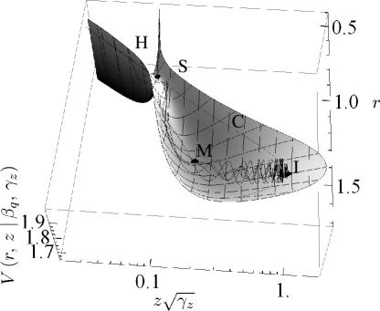
Figure 3: The effective potential for the variational approximation. This is a plot of the potential $V\left(r,\,z\,\left|\,\beta_{q},\,\gamma_{z}\right)\right.$ in Eq. (5) for $\gamma_{z}=1/50$ and $\beta_{q}=0.903\beta_{\text{GS}}^{\text{V}}$. Here $\beta_{\text{GS}}^{\text{V}}$ is the value of $\beta$ at which potential $V$ ceases to have a local minimum at this $\gamma_{z}$ (i.e. $\beta_{\text{GS}}^{\text{V}}$ is the variational prediction for the ground-state critical value of the coupling, $\beta_{\text{GS}}$). Point M is the local minimum of the potential, while S is the saddle point. Region H marks the “potential hole” which, if the system ventures into it, leads to the collapse, driving both the radial and axial widths, $r$ and $z$, to zero. Dashed curve C is the equipotential level curve of the saddle point. The $(r,\,z)$ coordinates of point I correspond to the minimum of the potential for $\beta_{\text{i}}=0.0451\beta_{\text{GS}}^{\text{V}}$. The system is first prepared in this minimum (i.e., in its ground state for $\beta=\beta_{\text{i}}$), and then $\beta$ is quenched by a factor of $q=20$ to $\beta_{q}=0.903\beta_{\text{GS}}^{\text{V}}$. Since the kinetic energy is zero immediately after the quench, the post-quench potential energy at I is the total energy of the effective particle, and, in the particular case presented here, it will have enough energy to climb over the saddle point, making the system unstable in the framework of the variational model. For the system to be energetically protected against collapse (i.e., stable over infinite times) at this particular value of post-quench coupling $\beta_{q}$, the pre-quench coupling $\beta_{\text{i}}$ should be at least $(1/8)\beta_{\text{GS}}^{\text{V}}$, i.e., one should limit the quench factor to $q<7.22$. Even so, as the plotted trajectory shows, the system completes two full returns from the pericenter before finally making it over the saddle point and collapsing.

(a similar surface was discussed in Ref. Carr and Castin (2002)). For given $\gamma_{z}>0$ and $\beta<0$, the potential has the following features: if $|\beta|$ is not too large, there is a local minimum (corresponding to the GS of the system, and labeled M in Fig. 3), a negative singularity at the origin (corresponding to the “black hole” Ueda and Huang (1999) that forms as a result of the collapse, and labeled H in the figure), and a saddle point between the two (labeled S). We always quench from the GS of some potential; hence, the effective particle corresponding to the post-quench state always starts from the rest position. If the initial position (labeled I) belongs to the “stability region”—defined as the region that both (i) includes the local minimum and (ii) is bounded by the saddle-point equipotential curve (labeled C in the figure)—then the particle does not have enough energy to climb over the saddle point and eventually fall into the singularity at the origin; hence, the system is stable against collapse. On the other hand, if I is outside the stability region, the collapse is energetically allowed. However, the particle’s trajectory may, initially at least, keep missing the singularity. Intuitively, however, one may believe that this would not continue forever: as the system is far from integrability, it should be ergodic enough for almost every trajectory, whose energy is larger than the value of potential $V$ at S, to pass, sooner or later, too close to the origin and be sucked into the collapse singularity. Therefore, quenches that place I outside the stability region always result in a system that either collapses immediately, or is effectively metastable, collapsing in a finite time. For example, in Fig. 3, we see a trajectory that misses the singularity twice before finally being sucked into it on the third approach; we found that small changes in the parameters can make a difference in which approach to the saddle point turns into a collapse.

As $|\beta|$ grows larger, the local minimum M and the saddle point S become closer, until they coalesce at some critical value $\beta_{\text{GS}}^{\text{V}}$. For still larger values of $|\beta|$, the potential contains no local minima and no saddle points, and the respective particle is never energetically protected from falling into the singularity (in particular, $\beta_{\text{GS}}^{\text{V}}$ is the variational estimate of $\beta_{\text{GS}}$). Similarly to the reasoning above, the non-integrability of the system then suggests that it will, with probability $1$, collapse in a finite time, irrespective of the initial state. In this case, the system may nevertheless be effectively metastable for some time, prior to the eventual onset of the collapse—at least if the coupling strength is not much larger than its critical value. However, numerical integration of the variational equations of motion show that once the local minimum (and so the variational ground state) is gone, metastability is very weak. In contrast, it turns out that in the full GPE, metastability continues well beyond the point where the system has no stable ground state. This is why we will not quantitatively study metastability within the variational model. Instead, we will study two kinds of metastability below, using the full GPE. The informative aspects of the variational model, beyond the “mental picture” of Fig. 3, will be presented in Fig. 4. First, however, we need to explain what functions will be plotted there.

We introduce some functions corresponding to the quantities discussed above, namely $(r_{\text{{M}}}(\beta,\,\gamma_{z}),\,z_{\text{{M}}}(\beta,\,\gamma_{z}))$, $(r_{\text{{S}}}(\beta,\,\gamma_{z}),\,z_{\text{{S}}}(\beta,\,\gamma_{z}))$, and $\beta_{\text{GS}}^{\text{V}}(\gamma_{z})$, the meaning of which is self-explanatory. The superscript “V” in the last item implies that it is produced by the variational model, as opposed to $\beta_{\text{GS}}(\gamma_{z})$, whose values are generated by the full GPE.

Our procedure that models the quench dynamics is defined as follows. (1) Fix a value of the aspect ratio, say $\gamma_{z,0}$, and of the coupling constant, say $\beta_{\text{i}}$. The latter must be sub-critical, $\left|\beta_{\text{i}}\right|<\left|\beta_{\text{GS}}^{\text{V}}(\gamma_{z})\right|$, so that there is a stable GS for this value of $\beta$. (2) Find the GS for these values of $\gamma_{z}$ and $\beta$, i.e., coordinates $(r_{\text{{M}}}(\beta_{\text{i}},\,\gamma_{z,0}),\,z_{\text{{M}}}(\beta_{\text{i}},\,\gamma_{z,0}))$ of the minimum of the potential $V\left(r,\,z\,\left|\,\beta_{\text{i}},\,\gamma_{z,0}\right)\right.$. (3) Change the coupling constant to $\beta_{q}=q\beta_{\text{i}}$, with quench factor $q>1$. In order for the following steps to make sense, we must have $\left|\beta_{q}\right|\leqslant\left|\beta_{\text{GS}}^{\text{V}}(\gamma_{z})\right|$ (as mentioned above, in terms of the variational model, the system can be, at best, metastable if $\left|\beta\right|>\left|\beta_{\text{GS}}^{\text{V}}\right|$; below, we study metastability using the full GPE). (4) Find coordinates $(r_{\text{{S}}}(\beta_{q},\,\gamma_{z,0}),\,z_{\text{{S}}}(\beta_{q},\,\gamma_{z,0}))$ of the saddle point of the post-quench potential, $V\left(r,\,z\,\left|\,\beta_{q},\,\gamma_{z,0}\right)\right.$. Now we define our long-time stability criterion in the framework of the variational model: $V\left(r_{\text{{M}}}(\beta_{\text{i}},\,\gamma_{z,0}),\,z_{\text{{M}}}(\beta_{\text{i}},\,\gamma_{z,0})\,\left|\,\beta_{q},\,\gamma_{z,0}\right)\right.<V\left(r_{\text{{S}}}(\beta_{q},\,\gamma_{z,0}),\,z_{\text{{S}}}(\beta_{q},\,\gamma_{z,0})\,\left|\,\beta_{q},\,\gamma_{z,0}\right)\right.$ (note that the argument of $r_{\text{{M}}}$ and $z_{\text{{M}}}$ is $\beta_{\text{i}}$, while everywhere else it is $\beta_{q}$). If this condition holds, then the effective particle (which, post-quench, starts motion from the initial rest position) does not have enough energy to climb over the saddle point and fall into the potential hole. In this case, the variational model predicts that the system is stable against collapse at all times. Accordingly, the critical quenched coupling strength $\beta_{(\infty)}^{\text{V}}(\beta,\,\gamma_{z})$ is defined as a solution of the equation $V\left(r_{\text{{M}}}(\beta,\,\gamma_{z}),\,z_{\text{{M}}}(\beta,\,\gamma_{z})\,\left|\,\smash{\beta}_{(\infty)}^{\text{V}},\,\gamma_{z}\right)\right.=V\left(r_{\text{{S}}}(\smash{\beta}_{(\infty)}^{\text{V}},\,\gamma_{z}),\,z_{\text{{S}}}(\smash{\beta}_{(\infty)}^{\text{V}},\,\gamma_{z})\,\left|\,\smash{\beta}_{(\infty)}^{\text{V}},\,\gamma_{z}\right)\right.$.

The results of the variational model are summarized in Fig. 4. The conclusions are as follows. In Fig. 4(a), we see that the maximal absolute value of the post-quench coupling strength (such that the system is still stable against the collapse even for infinite times, in the variational model) is about $90\%$ of $\beta_{\text{GS}}^{\text{V}}(\gamma_{z})$ for small initial $\beta_{\text{i}}$, and it steadily increases up to $100\%$ as $\beta_{\text{i}}$ approaches $\beta_{\text{GS}}^{\text{V}}$, while the dependence on $\gamma_{z}$ is weak. Figure 4(b) implies that $\beta_{\text{GS}}^{\text{V}}$ overestimates the numerically found value of $|\beta_{\text{GS}}|,$ which is given in Table 1, by about $15\%$. Figures 4(c)-(f) show how $r_{\text{{S}}}$ and $z_{\text{{S}}}$, and $r_{\text{{M}}}$ and $z_{\text{{M}}}$, depend on $\beta$ and $\gamma_{z}$. Note that, as $\beta$ approaches $\beta_{\text{GS}}^{\text{V}}(\gamma_{z})$, $(r_{\text{{S}}},\,z_{\text{{S}}})$ and $(r_{\text{{M}}},\,z_{\text{{M}}})$ approach a common value, which is close to $(1,\,1)$. Only $z_{\text{{M}}}$ has a strong dependence on $\gamma_{z}$, and only for small values of $\gamma_{z}$ and $\beta$. In general, $r_{\text{{S}}}$ and $z_{\text{{S}}}$ are always roughly equal to each other. A simple explanation of this fact, which is arguably correct within the variational model, would go as follows: reaching the saddle point heralds the beginning of the collapse, and, in the course of the collapse, the attractive interactions are overwhelming everything else. Hence, the shape of the collapsing condensate should be nearly spherical, at least within the variational model. Figures 4(c) and (d) suggest that $\beta/\beta_{\text{GS}}^{\text{V}}$ is a good estimate of this approximately common value of $r_{\text{{S}}}$ and $z_{\text{{S}}}$.

We should note that the true asymptotic shape of a collapsing single-peak solution of the GPE has been extensively studied in the literature, and there is solid evidence that the collapse is indeed asymptotically isotropic in its final stages. However, there are also some results that contradict this claim, so that open questions still remain (Appendix C).

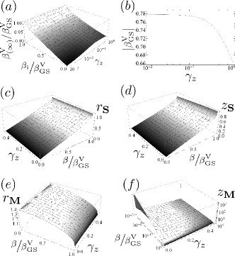
Figure 4: Results from the variational model. (a) Within the variational theory, $\beta_{(\infty)}^{\text{V}}$ is the strongest $\beta_{q}$ to which we can quench and still have the system be energetically protected from collapse. It is a variational estimate of $\beta_{(\infty)}$. Here we plot how $\beta_{(\infty)}^{\text{V}}$ depends on the aspect ratio $\gamma_{z}$ and the pre-quench coupling $\beta_{\text{i}}$. (b)$\left|\beta_{\text{GS}}^{\text{V}}\right|$ is the least upper bound on $\left|\beta\right|$ such that potential $V$ in Eq. (5) still has a minimum. It is a function of $\gamma_{z}$, and is a variational estimate of $\left|\beta_{\text{GS}}\right|$. Comparing these results to those in Table 1, we see that the variational model overestimates $\left|\beta_{\text{GS}}\right|$ by about 15%. In (c) we plot the $r$-coordinate of the saddle point of the potential as a function of $\beta$ and $\gamma_{z}$. In (d)-(f), we do the same, respectively, for the $z$-coordinate of the saddle point, and the $r$- and $z$-coordinates of the potential minimum.

III Numerical integration of the GPE

The above variational model suggests that, even following a quench that results in a supercritical coupling strength, the system may still avoid collapse for some time, in a metastable state. By means of numerical methods, we aim to address the following narrow but fundamental questions: (1) What are the critical quenches that result in an immediate collapse of the system, i.e., without even a single return from the pericenter? (2) What are the critical quenches that result in at least two returns from the pericenter (i.e., one full cycle of the breathing)? (3) In the latter case, as we approach the critical quench, what is the limiting value of the time interval between the first two passages through the pericenter?

The simulations were run by means of the GPELab toolbox for MatLab Antoine and Duboscq (2014, 2015), which necessitates the use of a uniform spatial grid. This makes it difficult to study large quenches, because the system is initially broad (requiring a large computational domain), and then drastically shrinks, requiring a closely spaced grid. For these reasons, we here report the results for the pre-quench coupling strength $\geq(1/8)\left|\beta_{\text{GS}}\right|$.

III.1 Critical quench leading to the immediate collapse

For every $\gamma_{z}$ and every initial $\beta_{\text{i}}$, we steadily increase the quench factor $q$ and keep track of $A_{\text{max,1}}$, the peak height at the first post-quench pericenter. The collapse corresponds to a divergence in $A_{\text{max,1}}$, and since the whole process looks like a critical phenomenon, one may expect to see a power-law behavior. Indeed, we always find that, as the quench factors approach the critical value, the peak heights feature a power-law singularity:

$$A_{\text{max,1}}(\beta_{q})=\frac{a}{(b-\beta_{q})^{c}}\,,$$ (6)

with $c>0$. We identify parameter $b$ with the $\beta$ corresponding to the critical quench, $\beta_{(1)}$; see a typical example in Fig. 5.

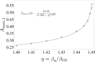
Figure 5: The power-law singularity for the first-pericenter peak heights. We start from the ground state for $\gamma_{z}=1/1000$ and $\beta_{\text{i}}=(1/8)\beta_{\text{GS}}(\gamma_{z})$, and then quench to $\beta_{q}$. The open circles are the values of $A_{\text{max,1}}$, the peak height at the first post-quench pericenter (for example, in Fig. 2 this corresponds to the peak height $\approx 0.16$, attained at $t=28$) The solid line is a fit to the power law, whose analytical form is also displayed. From the fit, we conclude that the critical value of $\beta_{q}$ is about $1.45\beta_{\text{GS}}$.

The results for $\beta_{(1)}$ obtained this way are summarized in Table 2.

$\bm{\displaystyle\beta_{(1)}/\beta_{\text{GS}}}$

as a function of $\bm{\displaystyle\beta_{\text{i}}/\beta_{\text{GS}}}$ and $\bm{\displaystyle\gamma_{z}}$

$0.125$ 0.3 0.5 0.7 0.9 0 $1.47$ $1.11$ 1.013 0.987 0.991 1/1000 $1.45$ $1.11$ 1.013 0.987 0.992 1/300 $1.34$ $1.11$ 1.013 0.987 0.992 1/50 $1.06$ $1.05$ 1.005 0.986 0.992

Table 2: The values of $\beta_{(1)}\left(\beta_{\text{i}},\,\gamma_{z}\right)/\beta_{\text{GS}}\left(\gamma_{z}\right)$, where $\left|\beta_{(1)}\left(\beta_{\text{i}},\,\gamma_{z}\right)\right|$ is the largest value of post-quench $\left|\beta\right|$ (i.e. of $\left|\beta_{q}\right|$) to which we can quench, starting from the ground state at $\beta_{\text{i}}$ and $\gamma_{z}$, so that, prior to collapse, the breather performs at least one return from the pericenter. For example, starting from the ground state at $\gamma_{z}=1/300$ and $\beta_{\text{i}}=0.3\beta_{\text{GS}}$ (where, according to Table 1, $\beta_{\text{GS}}=-0.676$), the system will immediately collapse if we quench to a $\left|\beta_{q}\right|>1.11\left|\beta_{\text{GS}}\right|$, whereas it will manage at least one return from the pericenter if $\left|\beta_{q}\right|<1.11\left|\beta_{\text{GS}}\right|$.

$\bm{\displaystyle\beta_{(2)}/\beta_{\text{GS}}\left(\gamma_{z}\right)}$

as a function of $\bm{\displaystyle\beta_{\text{i}}/\beta_{\text{GS}}}$ and $\bm{\displaystyle\gamma_{z}}$

$0.125$ 0.3 0.5 0.7 0.9 0 $1.233$ $1.076$ 1.013 0.987 0.991 1/1000 $1.217$ $1.075$ 1.016 0.987 0.992 1/300 $1.144$ $1.074$ 1.013 0.987 0.992 1/50 $1.031$ $1.032$ 1.005 0.986 0.992

Table 3: The values of $\beta_{(2)}\left(\beta_{\text{i}},\,\gamma_{z}\right)/\beta_{\text{GS}}\left(\gamma_{z}\right)$, where $\left|\beta_{(2)}\left(\beta_{\text{i}},\,\gamma_{z}\right)\right|$ is the largest value of the post-quench $\left|\beta\right|$ (i.e. of $\left|\beta_{q}\right|$) to which we can quench, starting from the ground state at $\beta_{\text{i}}$ and $\gamma_{z}$, and still have the breather the breather completing at least two returns from the pericenter. For $\beta_{\text{i}}/\beta_{\text{GS}}\geqslant 0.5$, the entries coincide with the corresponding ones in Table 2, because it is the first approach to the pericenter that turns into a collapse (see text).

Time interval between first two pericenters
as a function of $\bm{\displaystyle\beta_{\text{i}}/\beta_{\text{GS}}}$ and $\bm{\displaystyle\gamma_{z}}$
in the limit as $\bm{\beta_{q}\to\beta_{(2)}}$

0.125 0.3 0.5 0.7 0.9 0 72 29 41 26 20 1/1000 71 30 29 38 27 1/300 61 29 33 26 27 1/50 31 28 27 26 23

Table 4: The time intervals between the breather’s first and second traversal of the breathing pericenter, in the limit as post-quench $\beta$ (i.e $\beta_{q}$) approaches $\beta_{(2)}$. We quench from the ground state at $\beta_{\text{i}}$ and $\gamma_{z}$.

We see that the largest critical values of the coupling strength—almost $50\%$ larger in magnitude than the corresponding GS critical values $\left|\beta_{\text{GS}}(\gamma_{z})\right|$—occur for small values of $\gamma_{z}$ and $\beta_{\text{i}}$. In other regimes, the critical value of the post-quench $\beta$ is close to $\beta_{\text{GS}}$: slightly larger than $\beta_{\text{GS}}$ if $\gamma_{z}$ is larger but $\beta_{\text{i}}$ is still small, and slightly smaller than $\beta_{\text{GS}}$ if $\beta_{\text{i}}$ is close to $\beta_{\text{GS}}$, regardless of the value of $\gamma_{z}$. The lack of dependence on $\gamma_{z}$ when $|\beta|$ is large makes sense, because when $\beta_{\text{i}}$ is close to $\beta_{\text{GS}}$, the GS has a very small size and a roughly spherical shape, as in this case the interactions completely dominate over the harmonic trapping.

III.2 Critical quench leading to the delayed collapse

Here we seek another kind of critical quench, determined by the largest value of the quench factor that still allows the system to return from the pericenter at least twice. As the quench increases, the collapse that prevents the system from accomplishing this may happen either on the second approach to the pericenter, or already on the first. In the latter case, the critical value of the post-quench coupling will be the same as in the previous section. Numerically, we observe that the second approach leads to collapse if the pre-quench coupling is weaker than about $\beta_{\text{i}}=(1/2)\beta_{\text{GS}}$, whereas if the pre-quench coupling is stronger than that, then the system collapses on the first approach. Therefore, there is a crossover $\beta_{\text{i}}$ at which the occurrence of the collapse switches from the second approach to the first. Thus we conclude that, except for the crossover point $\beta_{\text{i}}$, for any given $\gamma_{z}$ and $\beta_{\text{i}}$, as the critical quench is approached, the peak height increases, according to a singular power law, at exactly one of the pericenters. The variational model of Sec. II provides an intuitive reason for this: if a pericenter is a precursor of the collapse (in the sense that it turns into a collapse if we slightly increase the coupling strength), then the pericenter corresponds to the effective particle approaching the origin in a somewhat fine-tuned, a “just-right” way. As the quench continuously increases, it is not surprising that, eventually, one of the first two visits by the particle to the region around the origin starts to resemble the “just-right” way of the approach. But it would be surprising if this started to happen for both of the particle’s first two visits, the latter actually requiring another fine-tuning, this time in $\beta_{\text{i}}$, leading to the crossover $\beta_{\text{i}}$.

The critical value of the coupling can therefore be determined just as in the previous section: by monitoring, as the quench increases, the peak heights at the first two pericenters. Eventually, one of these heights will start to increase (considered as a function of the quench) according to a singular power law, and we can again use the curve-fitting method of Fig. 5 to figure out the critical value of the coupling strength. The corresponding results are summarized in Table 3.

As the quench keeps increasing, one can also keep track of the time interval between the first two pericenters. In the limit of the quench approaching the critical point, these time intervals converge to finite values, which are presented in Table 4.

IV Summary and outlook

We have numerically studied, within the mean-field (GPE-based) approximation, the dynamical collapse of a class of excited states in a BEC with attractive two-body interactions [characterized by the interaction constant $\beta<0$ in Eq. (7)], in a cigar-shaped potential trap of aspect ratio $\gamma_{z}$. The excited states in question are produced by preparing the system in its GS (ground state) for some $(\gamma_{z},\,\beta_{\text{i}})$, and then quenching the coupling strength to some $\beta_{q}$ with a larger absolute value. For relatively weak quenches, the result is a stable excited state of the BEC that undergoes oscillations in its width and amplitude, i.e., a breather. When the width of the system, viewed as a function of time, attains a minimum or maximum, we say that the system is at its “pericenter” or “apocenter,” respectively. On the other hand, for very strong quenches, the system collapses immediately. For intermediate quenches, the system becomes metastable, exhibiting several pericenter-apocenter breathing cycles before collapsing. We have tabulated, for a range of values of $\gamma_{z}$ and $\beta_{\text{i}}$, the following quantities: (1) the smallest $\left|\beta_{q}\right|$ starting from which the collapse occurs immediately (Table 2); (2) the smallest $\left|\beta_{q}\right|$ at which the system collapses before completing two returns from the pericenter, i.e., in the course of its first or second shrinkage stage (Table 3); (3) the limiting value, as $\left|\beta_{q}\right|$ keeps increasing towards the critical value from Table 3, of the time interval between the first two pericenters (Table 4). The collapse is always identified by the following method: we monitor the peak height of the density profile at the pericenters of interest, as $\left|\beta_{q}\right|$ steadily increases. When $\beta_{q}$ gets close to the critical value, the pericenter peak height features a singular power-law dependence on $\beta_{q}$. By fitting the peak heights to the power-law approximation given by Eq. (6), we have found the critical value of $\beta_{q}$, see Fig. 5. In Sec. II, we have also studied the stability in the framework of a variational model, which offers useful intuition for the understanding of (near-)collapse dynamics. Moreover, this model provides the only currently available estimate for the critical value of the quench below which the system is stable for indefinitely long times [see Fig. 4(a)]: ignoring the weak dependence on the aspect ratio $\gamma_{z}$, the value of $\left|\beta\right|$ attained by the quench must fall below $\approx 90\%$ of $\left|\beta_{\text{GS}}(\gamma_{z})\right|$, for small initial $\beta_{\text{i}}$. This upper limit increases approximately linearly towards $100\%$ of $\beta_{\text{GS}}$ as $\beta_{\text{i}}$ approaches $\beta_{\text{GS}}$.

As a possible extension of the present work, one can study what kinds of parameter regimes allow for metastability on time scales at which the upcoming experiments may run. If they may be much longer than a few breathing cycles, or if the pre-quench interaction strength is weaker than $(1/8)\left|\beta_{\text{GS}}\right|$, the new theoretical studies may require more powerful computational resources than what is used in the present work.

On the other hand, if the time scales available to the simulations are sufficiently long, we envision studying chaotic dynamics of breathers. In particular, one can see in Fig. 6 that the breathing need not be periodic.

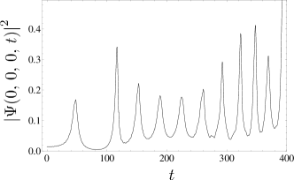
Figure 6: Nonperiodic breathing. The time evolution of the density’s peak height, following a quench from the ground state corresponding to parameters $(\gamma_{z}=0,\,\beta_{\text{i}}=0.125\beta_{\text{GS}})$ to $\beta_{q}=1.23\beta_{\text{GS}}$. The ten complete peaks correspond to pericenters; the 11th approach to the pericenter likely results in a collapse. The peak-to-peak time intervals go from $69$ for the first one, to $36$ for the second one, to $22$ for the ninth one (in the natural units).

The study of chaotic dynamics can be carried out at the level of dynamics of classical particles Zaslavsky (2005) (which actually corresponds to the variational model), and at the level of the classical-field dynamics Cvitanović (2000) (which corresponds to simulations of the full GPE). Eventually, in this system one may also be able to study quantum effects in chaos as well Wimberger (2014).

Next, an immediate objective may be to theoretically substantiate the intuitively expected and numerically observed singular power-law dependence of the pericenter peak heights on the coupling strength (Fig. 5). To the best of our knowledge, what has been extensively studied so far are self-similar solutions that exhibit power-law divergences as functions of time for a fixed supercritical interaction strength Sulem and Sulem (1999). In contrast, the power-law observed in Fig. 5 is a function of the interaction strength, as it is approaching the critical value from below.

Finally, for realistic description of experiments, one should include the loss and gain terms into the GPE. After all, when the BEC becomes unstable and collapses, it loses particles through three-body recombination. Thus closer the system comes to a collapse, the more relevent the loss terms are expected to be.

Appendix A The natural units

The “natural” units in this problem are those in which $\hbar=m=\omega_{r}=1$. It follows that the natural units of time, length, and mass, respectively, are $u_{T}=1/\omega_{r}$, $u_{L}=a_{\perp}=\sqrt{\hbar/(m\omega_{r})}$, and $u_{M}=m$. In the natural units, the GPE simplifies to

$$i\partial_{t}\Psi=-\frac{1}{2}\nabla^{2}\Psi+4\pi\,\beta\left|\Psi\right|^{2}\Psi$$

$$+\frac{1}{2}\left(x^{2}+y^{2}+\gamma_{z}^{2}z^{2}\right)\Psi\,,$$ (7)

where we used the fact that, in the natural units, $\omega_{z}$ has the numerical value $\gamma_{z}$, and $gN_{\text{a}}$ has the numerical value $4\pi\,\beta$. Of course, the above equation can also be interpreted as a change of variables: we introduce $\bar{x}=x/u_{L}$ (and similarly for the $y$- and $z$-components) and $\bar{t}=t/u_{T}$, and define the function $\bar{\Psi}(\bar{x},\,\bar{y},\,\bar{z},\,\bar{t})=u_{L}^{3/2}\,\Psi(u_{L}\bar{x},\,u_{L}\bar{y},\,u_{L}\bar{z},\,u_{T}\bar{t})$. Note that $\bar{\Psi}$ is normalized to 1 when integrated over $\bar{x}$, $\bar{y}$, and $\bar{z}$. We invert this, obtaining $\Psi(x,\,y,\,z,\,t)=u_{L}^{-3/2}\,\bar{\Psi}(x/u_{L},\,y/u_{L},\,z/u_{L},\,t/u_{T})$, and insert it into Eq. (2). We then express $x$, $y$, $z$, and $t$ in terms of $\bar{x}$, $\bar{y}$, $\bar{z}$, and $\bar{t}$, and simplify. We get a “barred” version of Eq. (7): that very equation except that all of $x$, $y$, $z$, $t$, and $\Psi$ have bars on them. But since $\bar{x}$ is the numerical value of $x$ when using natural units (and similarly for $y$, $z$, $t$ and $\Psi$), we see that the “barred” version of Eq. (7) is numerically identical to the actual Eq. (7) provided that in the latter we use the natural units. And we have already seen that in those units, Eq. (7) is numerically identical to Eq. (2).

Appendix B The “chirps” in the variational ansatz

It is well known that any variational ansatz for the wave function $\Psi$, like that in Eq. (4), must have a spatially-dependent phase whose functional form is $x^{2}$ times a function of time, plus the corresponding terms for the $y$- and $z$-components. (For example, in 1D, the functional form of the phase would be the same if instead of the Gaussian density profile one assumed a $\operatorname{sech}$-squared Desaix et al. (1991), which is the exact profile of a single GPE soliton.) Despite it being well-known, it has proved difficult to find a published reference that explains these facts. Reference Pérez-García et al. (1996) says that Ref. Desaix et al. (1991) has show that these terms ‘are essential if one wants to obtain reliable results’. From this one might expect that the latter reference compares what happens when these terms are excluded as compared to when they are present. But this is not what that reference does: instead, it compares the variational method (where such a term is simply included without comment) to a different, non-variational method. Indeed, we can see that completely excluding these terms leads to a stationary solution. Namely, excluding these terms is equivalent to setting $p_{x}=0$ (and similarly for the other two components); but since $p_{x}=m\dot{\mathit{w}}_{x}/\mathit{w}_{x}$, we get $\dot{\mathit{w}}_{x}=0$ (and similarly for the $x$- and $y$-components).

The closest to an explanation that we’ve been able to find in primary literature appears in Ref. Desaix et al. (1989), which says only that these chirps should expected from ‘[p]hysical intuition based on well-known results from linear and nonlinear pulse propagation theory’. On the other hand, Shaw Shaw (2004) suggests that these terms were motivated by the exact solution for a freely expanding Gaussan, a point to which we will return shortly.

Moreover, the literature seems to be in agreement Shaw (2004); Mikhailov (1999) that Ref. Anderson (1983) is the original reference for this functional form; however, in that paper it just appears without comment.

Here we will try to justify the presence and the functional form of these chirps in the Gaussan ansatz a bit more explicitly. First of all, the exact solution for a freely propagating Gaussian wavepacket with a stationary center of mass has this form Shaw (2004). Second, one can always write $\Psi=\sqrt{\rho}e^{iR/\hbar}$, where $\rho$ and $R$ are real-valued functions of $x$, $y$, $z$, and $t$. Inserting this into the GPE, the imaginary part of the resulting equation gives the equation of continuity, $\dot{\rho}+\vec{\nabla}\cdot\left(\rho\vec{\nabla}R/m\right)=0$. And from the latter it immediately follows that as soon as the density $\rho$ has any time dependence at all, the phase $R$ must have a nonzero spatial gradient and so must depend on the spatial coordinates. Moreover, in 1D it is easy to show that if $\rho$ is a Gaussian with width $\mathit{w}_{x}(t)$, then in fact the only way to satisfy the 1D continuity equation is to have $R=\frac{1}{2}x^{2}m\dot{\mathit{w}}_{x}/\mathit{w}_{x}$. The ansatz in Eq. (4) is a natural generalization of this, and it is easy to show that it does satisfy the 3D equation of continuity provided that $p_{y}=m\dot{\mathit{w}}_{y}/\mathit{w}_{y}$, and similarly for the $z$-components. Admittedly, we don’t have a proof that this functional form of the phase is the only possible one that will satisfy the 3D continuity equation when $\rho$ is a 3D gaussian, but it is a reasonable conjecture. Finally, this ansatz results in Eqs. (3), and they are known to give very good results when compared to numerics—for example for the frequencies of small oscillations around the equilibrium point Pérez-García et al. (1996), and for predictions for the onset of collapse, equilibrium widths, and dynamical evolution laws of the condensate parameters Pérez-García et al. (1997).

We hope that all these considerations provide a sufficient justification for the presence of the “chirps” in the variational ansatz.

Appendix C Asymptotic isotropy of a collapsing single-peak solution of the GPE

The true asymptotic shape of a collapsing single-peak solution of the GPE has been extensively studied in the literature, but open questions and even a degree of controversy still remain. On the one hand, it is known that asymptotically anisotropic collapsing solutions do formally exist Pelletier (1987) and have been reported in earlier numerically studies Degtyarev and Zakharov (1974). Moreover, these works gave physical arguments why it is that the anisotropic rather than isotropic collapsing solutions should be stable. On the other hand, not only has a numerical linear stability analysis showed that isotropic collapse is stable with respect to anisotropic disturbances Vlasov et al. (1989), but also the most recent high-quality numerical studies have never seen any asymptotically anisotropic collapsing solutions. Instead they have found that initially anisotropic one-peak solutions become isotropic near the collapse point, see Refs. Landman et al. (1991); Akrivis et al. (2003) and p. 130 of Ref. Sulem and Sulem (1999). Unfortunately, analytic results are still lacking.

Appendix D Discussion of results of Biasi et al. Biasi et al. (2017) in light of our own results

Biasi et al. Biasi et al. (2017) carried out a study very much related to ours, but with the following differences: 1. their system was radially symmetric, while ours is not; 2. their initial states were Gaussians, whereas for us they were the ground states of our system; 3. the number of spatial dimensions they considered went from two all the way to seven, whereas we only studied the 3D case; 4. their system was propagated until either it collapsed or some a priori specified maximal time was reached, no matter how many times it “bounced” from the pericenter; in our case, we concentrated on thresholds for transition between immediate collapse and collapse after a single bounce, and for transition between collapse after a single bounce and collapse after two. For some parameter choices their system was at these same transition points (in terms of how many bounces the system was able to complete before collapsing), and so in those particular cases (e.g. those labeled $\epsilon_{1}$ and $\epsilon_{2}$ in their Fig. 1), their system and ours do not differ with respect to the number of completed bounces; 5. they studied temporal evolution of the energy spectrum of low-lying modes as well as the mode-mode coupling coefficients, whereas we have not; 6. their criterion for collapse was apparent numerical divergence of the height of the central peak of the density distribution, whereas we used the procedure outlined in Sec. III.1.

The plots for $\epsilon_{1}$ and $\epsilon_{2}$ in their Fig. 1 are consistent with the general pattern we observed in our data, and they would correspond to $\beta_{(1)}/\beta_{\text{GS}}=0.67514$ (see our Table 2) and $\beta_{(2)}/\beta_{\text{GS}}=0.67510$ (see our Table 3), respectively. In our terms, we have that post-quench $\beta=\frac{1}{8}\sqrt{\frac{\pi}{2}}\epsilon^{2}\sigma^{3}$, where $\sigma$ is $\sqrt{2/5}$ in their Fig 1 and $\sqrt{1/2}$ in their Fig 2. Of course, since their initial states are not the same as ours, we wouldn’t be able to directly compare the results quantitatively even if we had done simulations for $\gamma_{z}=1$.

Their Fig. 2 shows that the total time to collapse is a very complicated non-monotonic function of the coupling strength $\epsilon$. We don’t have a plot corresponding to it, but we can make an educated guess as to what is happening. First of all, note that both the number of bounces and the time intervals between them generally change with changing $\epsilon$, which could easily result in a complicated plot. The most striking feature of their Fig. 2, however, are the sharp peaks in the time-to-collapse. These are likely the result of the system “lingering” at the threshold of collapse for that particular bounce, a bit like when an object climbs a hill with just barely enough energy to go over it. (As we have seen above, variationally speaking, actually it is not merely the question of total available energy, but also of the correct “aim” for the saddle point; see Sec. II.) And once $\epsilon$ passes (as it is lowered) this tricky threshold value, the collapses may start happening more quickly—until the next time $\epsilon$ is fine-tuned at the threshold of collapse during a particular bounce, which would produce another peak in their Fig. 2. The scenario we just outlined is consistent with their statement, ‘Roughly speaking, each step corresponds to a number of bounces in the harmonic potential. At the boundary between steps, $t_{c}$ presents a bump’. Unfortunately, we cannot confirm this scenario from our own data, because in effect we have the equivalent of just two points from their Fig. 2. Note that what is being varied in our Tables 2) and 3 are the aspect ratio and the initial state, both of which are completely fixed in their Fig. 2; if we fix them, then each table gives just one threshold value of post-quench $\beta$.

References

- Everitt et al. (2015) P. J. Everitt, M. A. Sooriyabandara, G. D. McDonald, K. S. Hardman, C. Quinlivan, M. Perumbil, P. Wigley, J. E. Debs, J. D. Close, C. C. Kuhn, and N. P. Robins, “Observation of breathers in an attractive Bose gas,” (2015), arXiv:1509.06844 [cond-mat.quant-gas] .
- Hulet (2016) R. G. Hulet, private communication (2016).
- Zakharov and Shabat (1972) V. F. Zakharov and A. B. Shabat, Zh. Eksp. Teor. Fiz. 61, 118 (1972), [Sov. Phys. JETP 34, 62 (1972)].
- Satsuma and Yajima (1974) J. Satsuma and N. Yajima, Prog. Theor. Phys. (Suppl.) 55, 284 (1974).
- Sakaguchi and Malomed (2004) H. Sakaguchi and B. A. Malomed, Phys. Rev. E 70, 066613 (2004).
- Prilepsky and Derevyanko (2007) J. E. Prilepsky and S. A. Derevyanko, Phys. Rev. E 75, 036616 (2007).
- Yanay et al. (2009) H. Yanay, L. Khaykovich, and B. A. Malomed, Chaos 19, 033145 (2009).
- Dunjko and Olshanii (2015) V. Dunjko and M. Olshanii, “Superheated integrability and multisoliton survival through scattering off barriers,” (2015), arXiv:1501.00075 [cond-mat.quant-gas] .
- Pethick and Smith (2008) C. J. Pethick and H. Smith, Bose-Einstein Condensation in Dilute Gases, 2nd ed. (Cambridge University Press, Cambridge, UK, 2008).