GRay2: A General Purpose Geodesic Integrator for Kerr Spacetimes

Abstract

Fast and accurate integration of geodesics in Kerr spacetimes is an important tool in modeling the orbits of stars and the transport of radiation in the vicinities of black holes. Most existing integration algorithms employ Boyer-Lindquist coordinates, which have coordinate singularities at the event horizon and along the poles. Handling the singularities requires special numerical treatment in these regions, often slows down the calculations, and may lead to inaccurate geodesics. We present here a new general-purpose geodesic integrator, GRay2, that overcomes these issues by employing the Cartesian form of Kerr-Schild coordinates. By performing particular mathematical manipulations of the geodesic equations and several optimizations, we develop an implementation of the Cartesian Kerr-Schild coordinates that outperforms calculations that use the seemingly simpler equations in Boyer-Lindquist coordinates. We also employ the OpenCL framework, which allows GRay2 to run on multi-core CPUs as well as on a wide range of GPU hardware accelerators, making the algorithm more versatile. We report numerous convergence tests and benchmark results for GRay2 for both time-like (particle) and null (photon) geodesics.

1. Introduction

Integrating geodesics of particles and photons in the spacetimes of Kerr black holes is an important aspect of theoretical modeling of various astrophysical phenomena, from the orbits of stars and compact objects around supermassive black holes (see, e.g., Alexander, 2017) to the transport of radiation through their accretion flows (see, e.g., Yuan & Narayan, 2014). Fast geodesic integrators are also critical in fitting data of, e.g., stars in orbit around the black hole in the center of the Milky Way (Boehle et al., 2016; Gillessen et al., 2017), of rotationally broadened fluorescence lines from accreting black holes in the X-rays (Miller, 2007), or of interferometric data taken with the Event Horizon Telescope that aims to take the first image of a supermassive black holes with horizon scale resolution (see, e.g., Doeleman et al., 2008, 2012).

Calculations of test-particle orbits (time-like geodesics) around black holes has been traditionally done in a post-Newtonian approximation, focusing on N-body effects (see, e.g., Brem et al., 2014; Hamers et al., 2014, for recent work), or by solving simultaneously for the dynamical spacetime of the cluster of particles (see Shapiro & Teukolsky, 1992, and references therein). More recently, fast algorithms have been developed that follow the orbits of test particles in stationary black-hole spacetimes, with no approximations (Yang & Wang, 2014; Zhang et al., 2015).

Integrations of null geodesics (ray tracing) in Kerr spacetimes can be traced back to Bardeen (1973), Cunningham (1975), and Luminet (1979), where the images of accretion disks and the outlines of the shadows of Schwarzschild and extreme Kerr black holes were first obtained. More recently, methods of combining polarized radiative transfer with ray tracing (see, e.g., Broderick & Blandford, 2003, 2004; Gammie & Leung, 2012; Younsi et al., 2012; Schnittman & Krolik, 2013) as well as a variety of open-source algorithms for fast radiative transfer calculations have been developed (see, e.g., Dexter & Agol, 2009; Dolence et al., 2009; Chan et al., 2013; Yang & Wang, 2013; Pu et al., 2016; Dexter, 2016).

In an earlier article, we described GRay (Chan et al., 2013), the first publicly available numerical algorithm that made explicit use of general-purpose computing on graphics processing units (GPU) for ray tracing in relativistic spacetimes. GRay uses the high computational horsepower of GPUs to speed up this computationally intensive problem. It achieved 1–2 orders of magnitude speed up compared traditional CPU-base algorithms and allowed us to generate large, high-cadence simulations of the observable properties of accreting black holes (Chan et al., 2015b, a; Psaltis et al., 2015; Kim et al., 2016; Ball et al., 2016; Medeiros et al., 2016a, b).

Even though GRay is very fast and efficient, it uses a standard physical setup of the ray-tracing problem as well as numerical methods that have a number of limitations. For example, like most of the other algorithms, GRay employs the Boyer-Lindquist (BL) coordinates to take advantage of the symmetry of the Kerr spacetime, which greatly simplifies the derivation and evaluation of the Christoffel symbols. However, the various coordinate singularities in the BL coordinates cause numerical difficulties. Moreover, as in many other algorithms, GRay uses the so called fast-light approximation (see, however, Dolence et al., 2009). This means that, when solving the radiative transfer equation along each ray, the fluid is assumed to be time independent, or equivalently, the speed of each photon is taken to be effectively infinite. This approximation greatly simplifies the algorithms because only a single snapshot of the underlying matter through which radiation propagates is needed in the radiative transfer calculation at each time step. However, this assumption affects the time variability properties of the simulations at the fastest timescales near the black-hole horizons (Dolence et al., 2009), which will be important in interpreting the upcoming observations with the Event Horizon Telescope (Kim et al., 2016; Medeiros et al., 2016a, b).

In order to overcome these difficulties, we describe here GRay2, a new open source, hardware accelerated, geodesic integration algorithm. We improve the geodesic integration in GRay2 by switching to the Cartesian form of Kerr-Schild (KS) coordinates, overcoming all coordinate singularities and increasing the overall accuracy of the calculations. We also switch to OpenCL, which allows GRay2 to run on multi-core CPUs as well as on a wide range of hardware accelerators, making the algorithm more versatile. Finally, GRay2 can handle both time-like (test particle) and null (photon) geodesics, making it applicable to calculations of both stellar orbits and radiative transfer.

In the next section, we discuss the limitations of using the BL coordinates and derive an optimized form of geodesic equations in the Cartesian KS coordinates. In section 2.2, we provide the details of using coordinate time instead of the affine parameter to integrate the geodesic equations. In section 2.3, we summarize the implementation details of GRay2. In section 3, we perform a convergence study using unstable spherical photon orbits and stable particle orbits. In section 4, we report benchmark results of GRay2 running on a wide range of CPUs and GPUs and demonstrate that GPUs can be up to two orders of magnitude faster than a single CPU core and that integrating in Cartesian KS coordinates can outperform integrating in BL coordinates. Finally, we summarize our findings in section 5.

2. The GRay2 Algorithm

2.1. Implementation of the Cartesian Kerr-Schild Coordinates

Letting $M$ and $a$ be the mass and spin parameter of a Kerr black hole, the Boyer-Lindquist line element reads

$$ds^{2} =-\left(1-\frac{2M\mathcal{r}}{\varrho^{2}}\right)d\mathcal{t}^{2}-\frac{4M\mathcal{r}a\sin^{2}\!\vartheta}{\varrho^{2}}d\varphi d\mathcal{t}+\frac{\varrho^{2}}{\varDelta}d\mathcal{r}^{2}$$

$$\!\!\!+\varrho^{2}d\vartheta^{2}+\left(\mathcal{r}^{2}+a^{2}+\frac{2M\mathcal{r}a^{2}\sin^{2}\!\vartheta}{\varrho^{2}}\right)\sin^{2}\!\vartheta d\varphi^{2},$$ (1)

where $\varrho^{2}\equiv\mathcal{r}^{2}+a^{2}\cos^{2}\vartheta$ and $\varDelta\equiv\mathcal{r}^{2}-2M\mathcal{r}+a^{2}$. The spherical polar nature of the BL coordinates introduces unnecessary coordinate singularities along the poles, in addition to the coordinate singularities at the event horizons. When integrating geodesics numerically, these coordinate singularities can cause significant difficulties. Although there exist algorithms to overcome these difficulties (see, e.g., the method introduced by Chan et al., 2013), the poles can still cause numerical problems such as slowing down the calculations, leading to inaccurate geodesics, and even crashing the algorithms for extreme cases such as computing a face-on image of a black hole accretion disk at inclination $i=0^{\circ}$.

In GRay2, we resolve the coordinate singularities by employing the Cartesian form of the KS coordinates

$$g_{\alpha\beta} =\eta_{\alpha\beta}+fl_{\alpha}l_{\beta},$$ (2)

where $\eta_{\alpha\beta}\equiv\mathrm{diag}(-1,1,1,1)$ is the Minkowski metric,

$$f =\frac{2r^{3}}{r^{4}+a^{2}z^{2}},$$ (3)

$$l_{\alpha} =\left(1,\frac{rx+ay}{r^{2}+a^{2}},\frac{ry-ax}{r^{2}+a^{2}},\frac{z}{r}\right),$$ (4)

and $r$ is defined implicitly by

$$x^{2}+y^{2}+z^{2}=r^{2}+a^{2}\left(1-z^{2}/r^{2}\right).$$ (5)

Its Cartesian nature not only completely avoids the coordinate singularities along the poles but requires no special treatment in the integrator. This is an advantage for implementing numerical integrators on modern hardware accelerators, such as GPUs, because these massive parallel stream processors use the Single-Instruction Multiple-Data (SIMD) paradigm, which are inefficient in handling branch instructions (i.e., conditional statements).

Besides the poles, both the spherical and Cartesian KS coordinates are also horizon-penetrating—there is no coordinate singularity at the event horizons. We can, in principle, integrate geodesics through the event horizon into the interior of the black hole. In fact, this property makes the spherical polar form of KS coordinates the default choice for many GRMHD codes (see, e.g., Gammie et al., 2003; Nagataki, 2009; Sa̧dowski et al., 2013; Ryan et al., 2015; White et al., 2016), as no special boundary treatment is required at the horizons.

Given that all the elements are non-zero in the Cartesian KS metric, this may seem at first to be a computationally very expensive coordinate system to work with. A rough operation-count goes as following. For the BL coordinates, there are 5 independent, non-zero elements in the metric, 10 independent elements in the metric derivative tensor $g_{\mu\nu,\alpha}$, and 20 independent Christoffel symbols. In contrast, in the Cartesian KS coordinates, we need to compute all 10 independent metric elements. The metric is time-independent but does not use any spatial symmetry, resulting in 30 independent elements in the metric derivative tensor. Since the metric derivative tensor tends to be the most complicated part of the calculation, this suggests that the computation of the 40 Christoffel symbols in the KS coordinates requires roughly 3 times more operations than in the BL coordinates. Therefore, we expect solving the geodesic equations in the Cartesian KS coordinates to be at least 3 times more expensive than in the BL coordinates.

For each geodesic, we need to solve all four second-order ordinary differential equations, if we integrate with respect to the affine parameter $\lambda$. Comparing to the methods that use the Killing vectors (see, e.g., Psaltis & Johannsen, 2012; Chan et al., 2013), this is a

$$\frac{2\times(8~{}\mbox{variables})}{2\times(6~{}\mbox{variables})+(1~{}\mbox{constant})}-1=23\%$$ (6)

increase in the bandwidth requirement. Nevertheless, as we will show in our benchmarks, geodesic integration is in general compute-bounded, meaning that the performance is limited by the speed of the computation and not by the speed of transferring data. Alternatively, we can also integrate the geodesic equations with respect to the coordinate time $t$ (see next section). This way, the number of dynamic variables reduces to six, which is the same as for GRay (Chan et al., 2013).

One of the important improvements in GRay2 is that, by a series of mathematical manipulations and regrouping, we significantly reduce the operation-count of the geodesic equations in the Cartesian KS coordinates. Let $\lambda$ be the affine parameter and $\dot{x}^{\mu}\equiv dx^{\mu}/d\lambda$. Our manipulations start by realizing that, although the Christoffel symbols $\varGamma^{\mu}_{\alpha\beta}$ provide an elegant form of writing the geodesic equations

$$\ddot{x}^{\mu} =-\varGamma^{\mu}_{\alpha\beta}\dot{x}^{\alpha}\dot{x}^{\beta},$$ (7)

it is actually more efficient to go back a step and write the equations in terms of the metric derivative tensor as

$$\ddot{x}^{\mu} =-\frac{1}{2}g^{\mu\nu}(g_{\nu\alpha,\beta}+g_{\nu\beta,\alpha}-g_{\alpha\beta,\nu})\dot{x}^{\alpha}\dot{x}^{\beta}$$ (8)

$$=-g^{\mu\nu}g_{\nu\alpha,\beta}\dot{x}^{\alpha}\dot{x}^{\beta}+\frac{1}{2}g^{\mu\nu}g_{\alpha\beta,\nu}\dot{x}^{\alpha}\dot{x}^{\beta}.$$ (9)

We can combine the first two terms in equation (8) because the product of an anti-symmetric tensor and a symmetric tensor vanishes—there is no need to explicitly symmetrize $\alpha$ and $\beta$ for $g_{\nu\alpha,\beta}$ from a computational point of view. Furthermore, equation (9) can be written as following by replacing the indices $\nu\rightarrow\beta\rightarrow\alpha\rightarrow\gamma$ for the first term and $\nu\rightarrow\alpha\rightarrow\beta\rightarrow\gamma$ for the second term

$$\ddot{x}^{\mu} =-\left(g^{\mu\beta}\dot{x}^{\alpha}-\frac{1}{2}g^{\mu\alpha}\dot{x}^{\beta}\right)g_{\beta\gamma,\alpha}\dot{x}^{\gamma}.$$ (10)

For each geodesic, $\dot{x}^{\mu}$ depend only on $\lambda$. Although we still need to evaluate all 30 independent non-zero elements of $g_{\beta\gamma,\alpha}$, we can store their results into the 12 non-zero elements the term outside the parenthesis in the above equation and reuse them in the summation of each $\mu$. Therefore, even in this general form without specifying a metric, the geodesic equations are in fact simpler than how they look, at least in terms of operation-count.

Next, by substituting the definition of the Cartesian KS metric (2) into equation (10), we obtain

$$\ddot{x}^{\mu} =-\left(\eta^{\mu\beta}\dot{x}^{\alpha}-\frac{1}{2}\eta^{\mu\alpha}\dot{x}^{\beta}\right)\dot{x}_{\beta,\alpha}+Fl^{\mu}$$ (11)

with

$$F \equiv f\left(l^{\beta}\dot{x}^{\alpha}-\frac{1}{2}l^{\alpha}\dot{x}^{\beta}\right)\dot{x}_{\beta,\alpha}.$$ (12)

In the above equations, the Minkowski metric $\eta^{\mu\nu}$ effectively picks out different components of the derivative tensor and applies different signs. Hence, we can split the equations and optimize them further as

$$\ddot{x}^{0} =\dot{x}^{\alpha}\dot{x}_{0,\alpha}-F,$$ (13)

$$\ddot{x}^{i} =-\dot{x}^{\alpha}\left(\dot{x}_{i,\alpha}-\frac{1}{2}\dot{x}_{\alpha,i}\right)+Fl^{i}.$$ (14)

Note that the positions of the indices 0 and $i$ do not match on the two sides of the above equations. This is not an error; equations (13) and (14) are no longer tensor equations.

In the above new form, the right hand sides (RHS) of the geodesic equations in the Cartesian KS coordinates have only $\sim 65\%$ more floating-point operations than in the BL coordinates. This is less than half of the operations compared to our rough estimate. Furthermore, the evaluation of the RHS uses many matrix-vector products, which are optimized in modern hardware. Indeed, as we show below, our benchmarks (Table 2 and 3) show that using the Cartesian KS on discrete GPUs can outperform its BL counterpart.

2.2. Coordinate Time Integration

In order to efficiently overcome the fast-light approximation, we need to control the integration of a geodesic to a targeted time according to the GRMHD simulations, which are usually performed in the spherical KS coordinates (see, e.g., Gammie et al., 2003; Sa̧dowski et al., 2013). This minimizes both the data reading and memory overhead by requiring only sequential reading with at most two snapshots in memory. In addition, we can take advantage of the fact that GPUs have special purpose hardware for accelerating interpolation, which makes accessing GRMHD simulations essentially free of overhead.

In GRay2, we develop two classes of methods to integrate the geodesic equations to a target KS coordinate time: (i) by directly integrating the geodesics with respect to the KS coordinate time and (ii) by applying different root finders to the numerical solutions to match the targeted time. In this section, we will limit our discussion to method (i) and derive the geodesic equations in terms of the KS coordinate time. Again, these equations are used in GRay2 mainly to overcome the fast-light approximation. Although they also reduce the required bandwidth of the geodesic integrator, the performance impact is very minor.

Letting $v^{\mu}\equiv dx^{\mu}/dt$ and using the chain rule, it is straightforward to derive the geodesic equations in the following form

$$\frac{dv^{i}}{dt} =-\varGamma^{i}_{\alpha\beta}v^{\alpha}v^{\beta}+\varGamma^{0}_{\alpha\beta}v^{\alpha}v^{\beta}v^{i}.$$ (15)

Note that we only consider the spatial components of the geodesic equations. The time component $dv^{0}/dt=0$ is trivial and consistent with the spatial part of the equations (see, e.g., Will, 1993). Substituting the definition of the Christoffel symbols, we get

$$\frac{dv^{i}}{dt} =-\frac{1}{2}g^{\prime i\nu}(g_{\nu\alpha,\beta}+g_{\nu\beta,\alpha}-g_{\alpha\beta,\nu})v^{\alpha}v^{\beta},$$ (16)

where $g^{\prime i\nu}\equiv g^{i\nu}-v^{i}g^{0\nu}$. Equations (16) and (8) have the same form. Hence, the optimizations we carried out in the last section are still applicable; equation (16) can be optimized to the generic form

$$\frac{dv^{i}}{dt} =-\left(g^{\prime i\beta}v^{\alpha}-\frac{1}{2}g^{\prime i\alpha}v^{\beta}\right)g_{\beta\gamma,\alpha}v^{\gamma}.$$ (17)

Finally, substituting the definition of the Cartesian KS metric, we obtain

$$\frac{dv^{i}}{dt} =-v^{\alpha}\left(v_{i,\alpha}-\frac{1}{2}v_{\alpha,i}\right)+Fl^{i}$$

$$\hskip 102.0pt-(v^{\alpha}v_{0,\alpha}-F)v^{i}.$$ (18)

The first two terms in the RHS of the above equation (i.e., first line) match the RHS of equation (14), while the last term (i.e., second line) matches the RHS of equation (13). This is expected and in fact shows that integrating with respect to the affine parameter and coordinate time have the same computational complexity. Therefore, because numerically integrating geodesics is compute bounded, the choice between integrating with respect to the affine parameter or with respect to the coordinate time will depend on the application of GRay2 and not on the detailed performance of each method. If one cares only about calculating the shapes of geodesics, then using coordinate time will reduce the number of variables and save some bandwidth as shown by equation (6). If, on the other hand, the radiative transfer equation needs to be integrated along a geodesic, then using the affine parameter will give the gravitational redshift with no additional computations.

2.3. Additional Implementation Improvements

In addition to the improvements in the coordinate system and numerical scheme, we have made a number of additional implementation improvements in GRay2. One of them is the adoption of OpenCL, an open standard for parallel programming, for executing massively parallel jobs on heterogeneous platforms. Without any modification of the source code, GRay2 runs on multi-core CPUs as well as accelerators such as GPUs, Intel Xeon Phi, and potentially Field-Programmable Gate Arrays (FPGA).

Another significant change is the adoption of the high performance computing (HPC) framework lux (Chan, 2017) for software portability and run time optimizations. With lux, the algorithms in GRay2 are broken down into very small modules, with multiple implementations for each of them. This allows the users to easily construct an appropriate compilation of modules that are specific to each application. In addition, lux benchmarks the algorithms at run time and allows GRay2 to automatically migrate to the most efficient algorithm. Finally, lux allows GRay2 to use all hardware resources on a single computing node. It even automatically balances the work load across the CPU cores and accelerators.

A typical application of GRay2 is to render millions of mock images of accretion flows onto black holes based on the output of GRMHD simulations, for different model parameters, such as electron number density scale and the electron-to-ion temperature ratio(see, e.g., Chan et al., 2015b, a). Because a single mock image takes only a few seconds to render, there is no need to consider inter-node communication. Instead, millions of GRay2 jobs can be submitted at the same time and each job runs in parallel, independently from each other. With this “trivially parallelizable” user case in mind, OpenCL and lux allows GRay2 to run on a wide range of hardware and platforms. For example, one can compute part of the jobs on an Apple desktop, part of the jobs on a local HPC cluster with GPUs, part of the jobs in a supercomputing center with Xeon Phi, and the rest of the jobs in commercial clouds such as the Amazon Web Services. This flexibility allows us to to report benchmarks for the implementation of (i) different forms of the equations, (ii) different data structures, and (iii) different precisions in section 4.

Figure 1 shows a screenshot of GRay2 in its interactive mode, which allows for the simultaneous integration and visualization of geodesics in a black-hole spacetime.

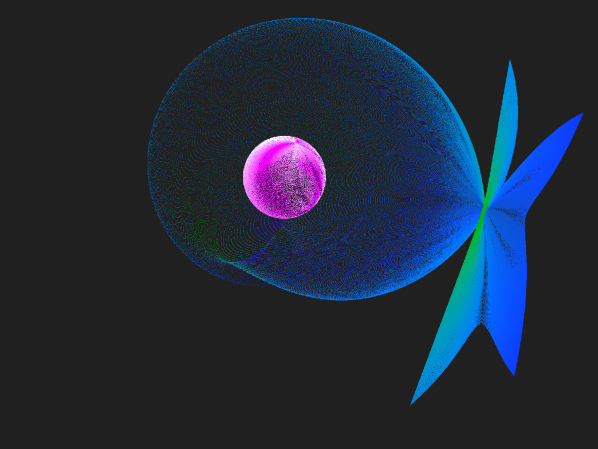
Figure 1.— A screenshot of GRay2 in its interactive mode, which allows a user to integrate and visualize the photon positions in real time. For this particular calculation, we set up a grid of photons originating at a large distance from a black hole with a spin of 0.999. This grid is deformed as it passes near the black hole event horizon. Some of the photons, shown in pink here, are trapped near the horizon. Some others, shown in green and blue, are deflected at large angles.

3. Convergence Tests

In this section, we perform a number of tests with GRay2, in situations that resemble expected realistic applications. By default, GRay2 uses the classic 4th-order Runge-Kutta scheme, which is very robust and provides fast (4th-order) convergence rates. We are interested here in its long term behavior in the Cartesian KS coordinates (see, e.g., Springel, 2005, for an explanation on the importance of long term behaviors of integrators). Typical gravitational deflection type of tests are not useful for this purpose because, in the Cartesian KS coordinates, the geodesic equations are trivial at large radii. In such cases, even though we could make the spatial interval of a geodesic arbitrarily long, the numerical error would still be dominated by a short segment of the geodesic near the black hole. This does not help to monitor the long term behavior of the integrators. Instead, we employ in our convergence tests closed, albeit often unstable, photon and particle orbits that can be integrated for long times.

3.1. Unstable Spherical Photon Orbits

Motivated by the interactive visualization by Stein (2016), we designed a set of tests using the unstable spherical photon orbits of Teo (2003). These orbits are non-trivial and are excellent for observing the long term behavior of the integrators. While their instability may seem like a problem at first, it makes the numerical errors accumulate (and grow) instead of canceling out and ensures that the worst numerical scenario is explored in our tests.

Teo (2003) showed that any spherical orbits must lie between the radii of the prograde and retrograde circular equatorial orbits,

$$r_{\mathrm{p}} \equiv 2M\left\{1+\cos\left[\frac{2}{3}\cos^{-1}\!\left(-\frac{|a|}{M}\right)\right]\right\},$$ (19)

$$r_{\mathrm{r}} \equiv 2M\left\{1+\cos\left[\frac{2}{3}\cos^{-1}\!\left(\frac{|a|}{M}\right)\right]\right\},$$ (20)

which satisfy the inequalities $M\leq r_{\mathrm{p}}\leq 3M\leq r_{\mathrm{r}}\leq 4M$. Therefore, our test orbits will be very close to the black hole—an ideal place to probe the performance of the integrators. Although no spherical orbits can pass the event horizon, some of them can pass the ergosphere,

$$r_{\mathrm{e}}=M+\sqrt{M^{2}-a^{2}\cos^{2}\theta}.$$ (21)

Note that we use the spherical KS coordinates $r$ and $\theta$ in the above equations because they are equal to the BL coordinates $\mathcal{r}$ and $\vartheta$.

Table 1Parameters For The Convergence Study with Null Geodesics.

Label	$a/M$	$r/M$	$\varPhi/M$	$Q/M^{2}$	​​​$\max(|\cos\theta|)$​​​	$\Delta\phi$
A	1	1.8 $\sqrt{2}$	1.36	12.8304	0.9387	12.0334
B	1	2 $\sqrt{2}$	1	16	0.9717	10.8428
C	1	$1+\sqrt{2}$	0	22.3137	1	3.1761
D	1	$1+\sqrt{3}$	-1	25.8564	0.9819	-3.7138
E	1	3 $\sqrt{2}$	-2	27	0.9352	-4.0728
F	1	$1+2\sqrt{2}$	-6	9.6274	0.4634	-4.7450

We list in Table 1 the parameters we use for our convergence study. The first column shows the label of the tests. We consider only the extreme Kerr black hole, $a=M$, and vary the radii of the spherical orbits. These two input parameters are listed in the second and third columns. With these two parameters, we can compute the normalized angular momentum $\varPhi$ and the normalized Carter’s constant $Q$ to initialize the orbits. For each test case, we also list, in the last two columns, the theoretical maximum altitude, $\max(|\cos\theta|)$, that the orbit can reach and the theoretical change in the azimuthal angle, $\Delta\phi$, within one complete polar oscillation. Although the spherical KS angle $\phi$ is different from the BL angle $\varphi$, their difference depends only on $r$ (see the Appendix). Hence, $\Delta\phi=\phi_{1}-\phi_{0}$ and $\Delta\varphi=\varphi_{1}-\varphi_{0}$ are equal to each other for the same spherical orbit.

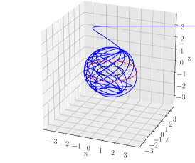
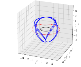
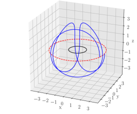
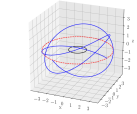
Figure 2.— Representative unstable spherical photon orbits around a black hole with $a=M$ used in our convergence study. (All panels) Blue lines are the photon orbits; black solid circles are the (physical) singularities; and red dashed circles mark the radii of the spherical orbits on the equatorial planes. All orbits start by moving upward from the positive $x$ sides of the red dashed circles. (Top-left) The orbit for Test A, which passes the ergosphere multiple times. Since the orbit is unstable, the small truncation and round off errors in the integrator get amplified as expected and the photon eventually leaves the $r=1.8M$ sphere and flies to infinity. (Top-right) The orbit for Test C. This is the special case where the photon exactly passes through the poles. See Figure 3 for a zoomed-in view of the north polar region. (Bottom-left) The orbit for Test E. The negative photon angular momentum cancels out the frame dragging effect exactly on the equator. (Bottom-right) The orbit for Test F. The initial angular momentum of the photon is negative enough that, unlike the other tests, the photon moves in the negative $\phi$ direction.

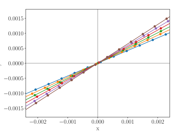
Figure 3.— A zoomed-in view of the north pole of Test A in the top-left panel of Figure 2. The solid circles are the actual steps of the 4th-order Runge-Kutta integrator with step size $\Delta\lambda=1/1024$ and the color lines simply join them together for readability. The first pass is the blue line from top-right, the second pass is the orange line from bottom left, etc.

Figure 2 shows a representative set of unstable spherical photon orbits that we used. For all panels, the blue lines are the photon orbits; the black solid circles are the (physical) singularities; and the red dashed circles mark the radii of the spherical orbits on the equatorial planes. All orbits start by moving upward from the positive $x$ sides of the red dashed circles.

The top-left panel shows Test A. In this case, the radius of the orbit is small enough and the polar momentum is large enough that the orbit oscillates in-and-out across the ergosphere, which GRay2 in Cartesian KS has no problem handling. Note that, since the orbit is unstable and we do not put any constraints on the integrator in GRay2, the small truncation and round off errors in the integrator get amplified as expected. Because of the accumulation of these numerical errors, the photon eventually leaves the $r=1.8M$ sphere and flies to infinity.

The top-right panel shows Test C, for which the whole orbit is now outside the ergosphere. Although the photon does not have any angular momentum in this case ($\varPhi=0$), the orbit is tilted on the equatorial plane because of frame dragging. Also, this is the special case for which the photon exactly passes the poles multiple times at $x=y=0$ and $z\approx\pm 2.41$. In Figure 3 we zoom into the north polar region of Test C. The solid circles are the actual steps of the 4th-order Runge-Kutta integrator with step size $\Delta\lambda=1/1024$ and the colored lines simply join them together for clarity. The first pass is the blue line from lower-left; the second pass is the orange line from top-right; etc. Again, the integrator has no problem handling the pole because there is no coordinate singularity in the Cartesian KS coordinates.

In the bottom-left panel, we plot the unstable spherical photon orbit for Test E. Although the photon angular momentum is negative, it cancels out the frame dragging effect exactly on the equatorial plane so the photon moves vertically when it passes the equator. In the bottom-right panel, we plot the photon orbit for Test F. This time, the initial angular momentum is negative enough that the photon finally moves in the negative $\phi$ direction.

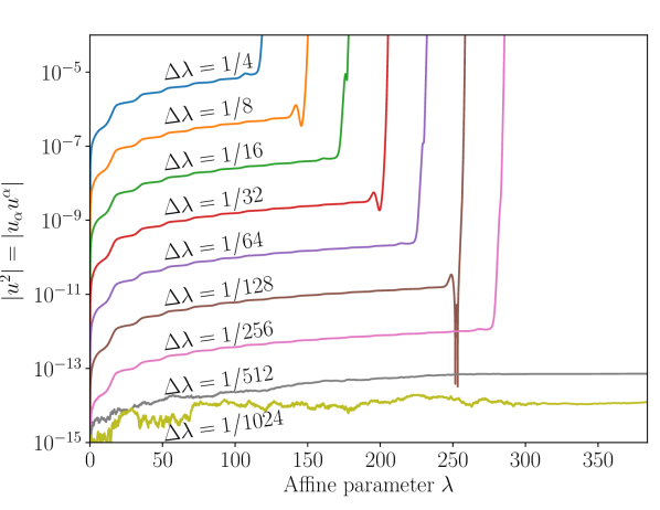
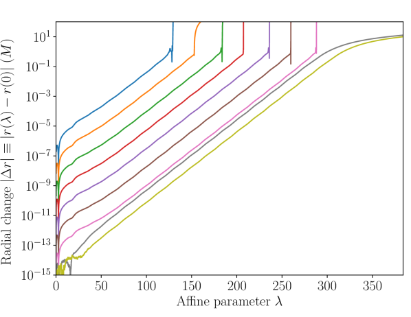
Figure 4.— (Left) The time evolution of $u^{2}=u_{\alpha}u^{\alpha}$ for Test A. We use nine different step sizes in this test, namely, $\Delta\lambda=1/4$, 1/8, …, 1/512, and 1/1024, which are labeled in the left panel. For all step sizes, $u^{2}$ is initially of order $10^{-16}$ and increases approximately linearly until the numerical solutions blow up. (Right) The change of the radius of the photon orbit as a function of $\lambda$. The color coding of the curves follows that of the left panel.

In Figure 4, we plot two of the error indicators for Test A. The left panel shows the time evolution of $u^{2}=u_{\alpha}u^{\alpha}$. It is a constant of motion and should remain zero for photons. In GRay2, because we integrate the geodesic equations without explicitly using any constants of motion, $u^{2}$ is, in principle, unconstrained in the numerical integration. Therefore, its value is a good measure of the numerical errors. We use nine different step sizes in this test, covering the range $\Delta\lambda=1/4$, 1/8, …, 1/512, and 1/1024, which are labeled on the left panel. For all step sizes, $u^{2}$ is initially of order $10^{-16}$ and increases approximately linearly until the numerical solutions blow up. Clearly, a smaller step size leads to smaller $u^{2}$ and, hence, smaller error.

To understand why the numerical solutions blow up, we plot the changes of the radius of the photon orbit as a function of $\lambda$ in the right panel. Recalling that the tests are for unstable spherical photon orbits, $|\Delta r|\equiv|r(\lambda)-r(0)|$ should grow exponentially, with an amplitude proportional to the perturbation—or to the numerical errors in our case—of the orbits. The coloring of the curves is identical to the left panel, namely, blue is for $\Delta\lambda=1/4$, orange is for $\Delta\lambda=1/8$, etc. All the curves grow as expected and blow up at around $|\Delta r|\sim 1$. This is not a coincidence. In fact, for all orbits except the gray and yellow ones, the photons approach the physical singularities as they depart from their spherical orbits. When they get very close to the singularities, the fixed time steps fail to integrate the geodesics, resulting in significant jumps in both $u^{2}$ and $\Delta r$. For the gray and yellow curves, the photons actually move away from the singularities as they depart from the spherical orbits. Therefore, although the photons approach infinity (linearly), $u^{2}$ always remain small.

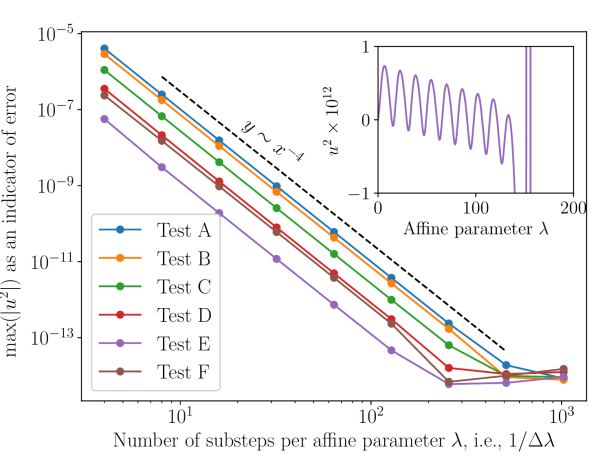
Figure 5.— Results of the convergence study using the integral of motion $u^{2}$. Here, we plot $\max(u^{2})$ for $0\leq\lambda<64$ for the six test problems we performed, as a function of the step $\Delta\lambda$ in the affine parameter. GRay2 converges at 4th order it used the 4th-order Runge-Kutta scheme. The amplitude of the error decreases as $r$ increases except for Test E. This is an artifact of the oscillatory behavior of $u^{2}$, in this test, shown in the inset.

In Figure 5, we summarize the convergence properties of our algorithm as quantified by the integral of motion $u^{2}$. We plot $\max(|u^{2}|)$ for $0\leq\lambda\leq 64$ for all six test problems. For each test problem, we change $\Delta\lambda$ in the range 1/4, 1/8, 1/16, …, to 1/1024. As Figure 4 already showed, the errors decrease as we use smaller step sizes and GRay2 converges at 4th order—an expected result because of the 4th-order Runge-Kutta scheme we are using.

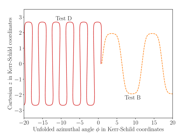
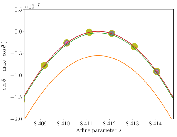
Figure 6.— (Left) Unfolded photon orbits in a cylindrical coordinate projection. The vertical axis is the Cartesian $z$ in the Kerr-Schild coordinates. The horizontal axis is the unfolded azimuthal angle $\phi$ in the Kerr-Schild coordinates. We only plot two representative curves here for Tests B and D. (Right) Zoom-in view of the first peak of Model B as a function of the affine parameter $\lambda$ with different step sizes. The solid circles are the actual output of the GRay2. For each step size, we fit a quadratic equation to the largest three circles. The quadratic equations are then plotted as the different curves here. The color scheme of the solid circles and the curves matches those of Figure 4.

For a more detailed test of the geodesics, in the left panel of Figure 6, we unfold the photon orbits in the azimuthal direction and plot the coordinate $z$ as a function of $\phi$. To avoid overlap between the oscillatory curves, we plot the orbits only for Test B and D. The photon in Test B has positive angular momentum, hence it moves toward positive $\phi$. In the same figure, the photon in Test D has a small negative angular momentum. Although its overall orbit points toward negative $\phi$, the photon changes its direction near the equator because of the stronger frame dragging effect there.

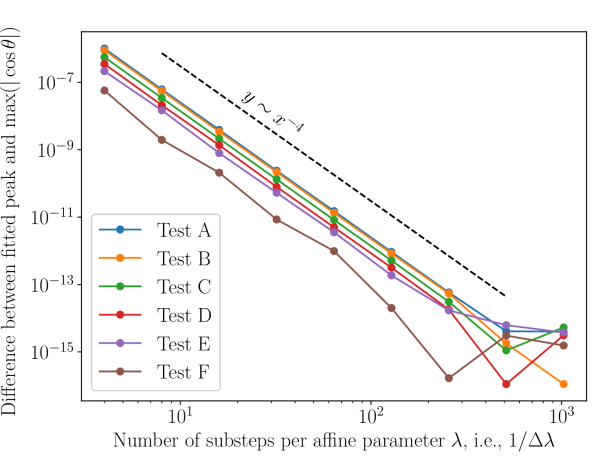
Figure 7.— Results of the convergence study using the maximum polar angles a photon reaches during its orbit. The plot is similar to Figure 5. It shows that the difference between the fitted peak value of the numerical solution converges to the analytical one at the expected 4-th order.

The peak values of the $z-$coordinate in the left panel of Figure 6 can be calculated analytically, are given in equation (8) in Teo (2003) and listed in the sixth column of our Table 1. We can use these as a second convergence test of GRay2. (Note that, for convenience, we plot in the following figures the maximum cosine of the polar angle, i.e., $\max|\cos\theta|$, instead of the maximum $z-$coordinate of each photon orbit). The numerical values at the local maxima depend strongly on the resolution because of sampling effect. This is illustrated in the right panel of Figure 6, where we zoom into the first peak of Model B as a function of the affine parameter $\lambda$ with different step sizes. The solid circles are the actual steps of the 4th-order Runge-Kutta scheme. It is clear that the circles are offset from the locations of the peaks. To overcome this sampling effect in polluting our convergence test, we fit a quadratic equation to the largest three points for each resolution. The curves in the right panel of Figure 6 correspond to these quadratic equations. From the plot, even the red curve with $\Delta\lambda=1/32$ is visually indistinguishable from the more accurate curves at this scale. Only at $\Delta\lambda=1/16$, the green curve starts to deviate from the more accurate curves. We compute the differences between the peak values of the fitted quadratic equations and the analytical values. The results are plotted in Figure 7, which shows again a 4th-order convergence rate for all the tests.

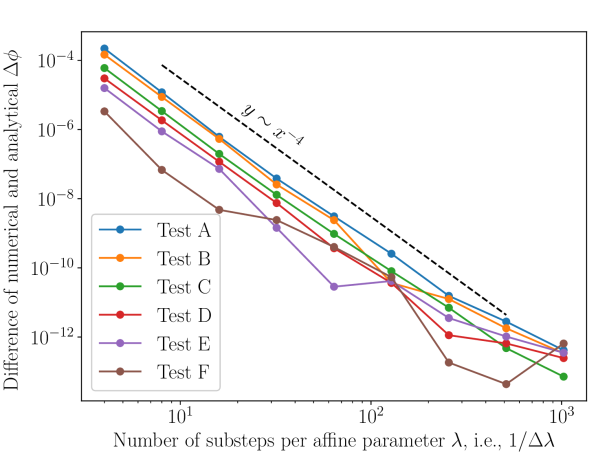
Figure 8.— Results of the convergence study using the change in the azimuth of the photon orbit during one complete oscillation in latitude. The plot is similar to Figure 5 and 7. It shows that the difference between the numerical and analytic values of $\Delta\phi$ converges at the expected 4-th order.

Our final convergence test uses another result from Teo (2003), who derived the equation to integrate the change in azimuth for one complete oscillation in latitude. Although there is still a sampling effect due to the change of step size, its resolution is much simpler. We simply use linear interpolation to obtain the root of $z(\phi)$ at the first complete cycle and subtract the initial coordinate $\phi$ from it. This numerical value is then compared with the numerical integration of equation (17) in Teo (2003). The final result is plotted in Figure 8, which again shows a 4th-order convergence rate for all the tests.

3.2. Stable Circular Particle Orbits

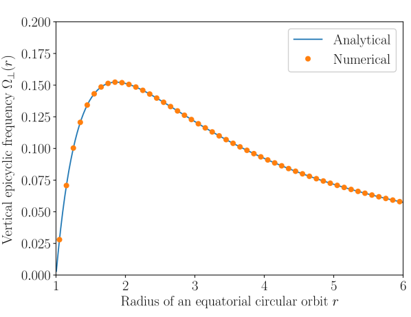
Figure 9.— Vertical epicyclic frequency as a function of orbital radius. We use GRay2 to integrate a nearly circular time-like geodesics around a black hole of spin $a=1$. We introduce a small initial vertical velocity $v_{z}=10^{-12}$ to induce vertical oscillation and precession. We then compare the numerical vertical epicyclic frequencies (orange circles) with its analytical expression (blue solid line). The fractional difference between the two curves at a radius $r<1.5$ is less than $10^{-13}$.

Since GRay2 makes no specific assumption about geodesics, it can integrate orbits for massive test particles, i.e., time-like geodesics, without any modification of the integrator. As a second set of convergence tests, we integrate stable, nearly circular orbits at different radii around a black hole with a spin of $a=1$.

Nearly circular orbits in general relativity precess because of the deviation of the effective gravitational potential from the Newtonian $1/r$ form. One can describe completely their motion along the three polar coordinates using three independent oscillatory frequencies, one azimuthal (the orbital frequency $\Omega$), one radial (the radial epicyclic frequency $\kappa$), and one vertical (the vertical epicyclic frequency $\Omega_{\perp}$). The radial epicyclic frequency vanishes at the location of the innermost stable circular orbit and becomes imaginary inside that radius. In the same region, the vertical epicyclic frequency is significantly smaller than the orbital frequency. All three frequencies for a nearly circular orbit can be calculated analytically (see, e.g., Silbergleit & Wagoner, 2008).

In order to force a small precession of the orbital plane of a test particle, we introduce a small vertical velocity, $v_{z}=10^{-12}$, to the initial conditions that would otherwise lead to a circular orbit. We then use the numerical orbit to calculate the vertical epicyclic frequency (as measured by an observer at infinity) and compare it to the analytic expression. In order to avoid the numerical effects described in the previous section, we perform linear interpolations between the calculated points in $z(t)$ and measure the time interval between successive maxima.

In Figure 9, we overplot the numerical measurement from GRay2 on the analytic expression, as a function of the radius of the orbit in BL coordinates. The numerical and analytical results are indistinguishable. In fact, for $r\lesssim 1.5$, the difference between the numerical and analytical results is less than $10^{-13}$. For all other convergence properties related to the test-particle orbits, we found no appreciable difference with the results shown earlier for the null geodesics.

4. Profiling and Benchmarks

Table 2Benchmark results for integration of null geodesics

Precision	Coordinates	Data Order	i7-3720QM	E5-2650$\times 2$	HD4000	GT650M	M2090	K20X	GTX780	Titan Black
Single	BL	AoS	43.1	6.07	2.99	2.49	0.597	0.223	0.174	0.167
Single	BL	SOA	49.4	6.01	2.98	2.89	0.597	0.219	0.170	0.175
Single	KS	AoS	57.5	6.27	4.53	2.69	0.995	0.420	0.311	0.297
Single	KS	SoA	54.8	6.20	4.55	2.31	0.995	0.422	0.315	0.309
Double	BL	AoS	55.4	16.6	—	70.6	—	3.90	6.44	1.65
Double	BL	SoA	56.7	16.2	—	80.6	—	3.90	6.44	1.66
Double	KS	AoS	66.0	17.4	—	59.1	—	2.41	6.95	1.15
Double	KS	SoA	63.1	17.5	—	59.0	—	2.40	6.96	1.15

In section 2.1, we reduced the operation-count of the geodesic equations in the Cartesian KS coordinates by a series of mathematical manipulations. This suggests that, theoretically, solving this optimized form of geodesic equations is not much more expensive than in the BL coordinates. In this section, we look at the actual benchmarks on different devices to support our assertions.

The most direct method to compare the performances of the geodesic equations in the Cartesian KS and BL forms is to look at the elapsed time for a single 4th-order Runge-Kutta time step of a single ray, which contains four evaluations of the RHS of the geodesic equations. However, modern accelerators such as GPUs are effectively vector processors. They are only efficient when a large number of threads are executed in parallel. In addition, these accelerators are not general purpose devices. Driving them requires a host—usually a full power CPU—to compile the kernels and send instructions and data to the devices. These overheads can sometimes be quite significant compared to the computations.

Table 3Benhcmarks Results for Null Geodesics

Precision	Coordinates	Data Order	i7-3720QM	E5-2650$\times$2	HD4000	GT650M	M2090	K20X	GTX780	Titan Black
Single	BL	AoS	2.25	16.0	32.5	39.0	163	436	558	582
Single	BL	SoA	1.95	16.0	32.3	33.3	161	439	566	549
Single	KS	AoS	1.74	16.0	22.2	37.3	101	239	323	338
Single	KS	SoA	1.81	16.0	21.8	42.9	99.7	235	315	321
Double	BL	AoS	4.79	16.0	—	3.76	—	68.1	41.2	161
Double	BL	SoA	4.57	16.0	—	3.22	—	66.5	40.3	156
Double	KS	AoS	4.22	16.0	—	4.71	—	116	40.1	242
Double	KS	SoA	4.44	16.0	—	4.75	—	117	40.2	243

We design our benchmarks to reduce the impacts of the above factors. Following the approach found in a typical application, we use GRay2 to integrate backwards null geodesics from an image at an initial radius $r=1024M$ toward a black hole of spin $a=0.999M$. The integration is performed by executing the same OpenCL kernel $\sim 64$ times, until all photons pass by or are close enough to the event horizon, or escape to distances larger than the initial radius. The kernel performs host-to-device communication once right after it starts the 4th-order Runge-Kutta methods with fixed step size 1024 times. It also performs device-to-host communications once more just before it ends. We measure the elapsed time between the instants when the kernel starts and ends. Typically, the elapsed time is reduced a bit after the first few kernel executions due to instruction loading and caching and then saturates toward a steady value.

Because the performance of GPUs is sensitive to how the computations are grouped and distributed to different sub-processors (for CPUs they are called “cores”; for nVidia GPUs they care called “multiprocessors”), in order to measure the peak performance, we repeat the above process with five different resolutions of images: $64\times 64$, $128\times 128$, $256\times 256$, $512\times 512$, and $1024\times 1024$, and allow lux’s run time performance tuning algorithm to choose the optimal workgroup size. We compute the elapsed time of a single step for each ray by dividing the shortest measured time by 1024 and the total number of rays.

We list the benchmark results in Table 2. The first three columns are the precision, the coordinate system, and the data-order used in GRay2, respectively. The numbers in all other columns are in nanoseconds. The 4th column is for a mobile/laptop 4-core CPU and the 5th column is for two 8-core server CPUs (i.e., 16 cores in total). The 6th column is for an Intel integrated graphics chip. The 7th–11th columns are for different nVidia GPUs.

All the tested processors, except Intel HD4000, support both single and double precisions. For nVidia’s Tesla M2090, our workstation failed to compile GRay2’s OpenCL kernel—this may be due to the limitation of the driver or a bug in the OpenCL implementation. For CPUs, the performance of single precision is only slightly (or a factor of a few) faster than for double precision. For the mobile and consumer graphics chips GT650M and GTX780, single precision is significantly faster—up to a factor of $\sim 28$—than double precision. This is no surprise. Single precision operations are good enough for computer graphics and gaming applications. Hence, a large number of transistors on these consumer graphics chips are used to perform single precision operations only. For the HPC specific GPU Tesla K20X and high-end graphics cards nVidia Titan Black, the performance difference between single and double precisions is less dramatic.

For single precision, integrating in the KS coordinates is slightly more expensive than in the BL coordinates but the difference is usually less than $\sim 70\%$ (except for K20X). This supports our estimate in section 2.1 that integrating in KS coordinates has roughly 65% more operations compared to integrating in BL coordinates. For double precision, it is interesting to note that, for most GPUs (except GTX780), KS integration is actually faster than BL integration by up to $\sim 40\%$. There are two main reasons for this. First, BL coordinates require evaluations of trigonometric functions, which are expensive in double precision. Second, the equations in KS are highly symmetric, which allows the compiler to optimize them by hardware-accelerated vector instructions.

Finally, there is no significant difference between the two different approaches to ordering the structures and arrays for these benchmarks. This is just an indication that our benchmarks successfully overcome memory access overhead and are able to reveal the actual computation performance.

In order to more easily read off the performance gain, we convert the elapsed time in Table 2 to speedups in Table 3. Larger numbers mean higher speedups. We use a single core of the E5-2650 CPU as our baseline. Hence, two E5-2650 CPUs give us 16 cores in the 5th column. For single precision, most of the GPUs are $100-600$ times faster than a single E5-2650 core. For double precision, although the speedups are not as large, the HPC specific Tesla K20X and high-end graphics cards nVidia Titan Black are still two orders of magnitude faster than a single E5-2650 core.

5. Summary

In this paper, we presented GRay2, a new open source, hardware-accelerated, general relativistic integrator for time-like and null geodesics. By using the Cartesian form of Kerr-Schild coordinates, integration in GRay2 avoids all coordinate singularities at the pole and at the horizon that are present in Boyer-Lindquist coordinates. Using a rearranged form of the geodesic equations (see equations [13] and [14]) makes the integrator in Cartesian KS coordinates as efficient as in BL coordinates. In addition, by using the OpenCL standard and the HPC framework lux, GRay2 runs optimally on a wide range of software platforms and hardware devices.

We carefully examined the properties of the numerical algorithm and showed that, for a number of different problems with known analytic solutions, it converges at the expected rate. We also report extensive performance benchmarks and show the significant (1-2 orders of magnitude) improvement in the efficiency of GRay2 when it is run on GPU architectures.

This algorithm is optimally suited for massively parallel integration of geodesics. It can be utilized for computing the transport of radiation through black hole accretion flows, the evolution of a cluster of particles in the vicinity of a black hole, or even direct particle or gyrokinetic simulations of plasmas in Kerr spacetimes.

References

- Alexander (2017) Alexander, T. 2017, ArXiv e-prints, arXiv:1701.04762
- Ball et al. (2016) Ball, D., Özel, F., Psaltis, D., & Chan, C. 2016, ApJ, 826, 77
- Bardeen (1973) Bardeen, J. M. 1973, in Black Holes (Les Astres Occlus), ed. C. Dewitt & B. S. Dewitt, 215–239
- Boehle et al. (2016) Boehle, A., Ghez, A. M., Schödel, R., et al. 2016, ApJ, 830, 17
- Brem et al. (2014) Brem, P., Amaro-Seoane, P., & Sopuerta, C. F. 2014, MNRAS, 437, 1259
- Broderick & Blandford (2003) Broderick, A., & Blandford, R. 2003, MNRAS, 342, 1280
- Broderick & Blandford (2004) —. 2004, MNRAS, 349, 994
- Chan et al. (2013) Chan, C., Psaltis, D., & Özel, F. 2013, ApJ, 777, 13
- Chan et al. (2015a) Chan, C., Psaltis, D., Özel, F., et al. 2015a, ApJ, 812, 103
- Chan et al. (2015b) Chan, C., Psaltis, D., Özel, F., Narayan, R., & Sa̧dowski, A. 2015b, ApJ, 799, 1
- Chan (2017) Chan, C. K. 2017, in preparation
- Cunningham (1975) Cunningham, C. T. 1975, ApJ, 202, 788
- Dexter (2016) Dexter, J. 2016, MNRAS, 462, 115
- Dexter & Agol (2009) Dexter, J., & Agol, E. 2009, ApJ, 696, 1616
- Doeleman et al. (2008) Doeleman, S. S., Weintroub, J., Rogers, A. E. E., et al. 2008, Nature, 455, 78
- Doeleman et al. (2012) Doeleman, S. S., Fish, V. L., Schenck, D. E., et al. 2012, Science, 338, 355
- Dolence et al. (2009) Dolence, J. C., Gammie, C. F., Mościbrodzka, M., & Leung, P. K. 2009, ApJS, 184, 387
- Gammie & Leung (2012) Gammie, C. F., & Leung, P. K. 2012, ApJ, 752, 123
- Gammie et al. (2003) Gammie, C. F., McKinney, J. C., & Tóth, G. 2003, ApJ, 589, 444
- Gillessen et al. (2017) Gillessen, S., Plewa, P. M., Eisenhauer, F., et al. 2017, ApJ, 837, 30
- Hamers et al. (2014) Hamers, A. S., Portegies Zwart, S. F., & Merritt, D. 2014, MNRAS, 443, 355
- Kim et al. (2016) Kim, J., Marrone, D. P., Chan, C., et al. 2016, ApJ, 832, 156
- Luminet (1979) Luminet, J.-P. 1979, A&A, 75, 228
- Medeiros et al. (2016a) Medeiros, L., Chan, C., Özel, F., et al. 2016a, ArXiv e-prints, arXiv:1610.03505
- Medeiros et al. (2016b) Medeiros, L., Chan, C., Ozel, F., et al. 2016b, ArXiv e-prints, arXiv:1601.06799
- Miller (2007) Miller, J. M. 2007, ARA&A, 45, 441
- Nagataki (2009) Nagataki, S. 2009, ApJ, 704, 937
- Psaltis & Johannsen (2012) Psaltis, D., & Johannsen, T. 2012, ApJ, 745, 1
- Psaltis et al. (2015) Psaltis, D., Özel, F., Chan, C., & Marrone, D. P. 2015, ApJ, 814, 115
- Pu et al. (2016) Pu, H.-Y., Yun, K., Younsi, Z., & Yoon, S.-J. 2016, ApJ, 820, 105
- Ryan et al. (2015) Ryan, B. R., Dolence, J. C., & Gammie, C. F. 2015, ApJ, 807, 31
- Sa̧dowski et al. (2013) Sa̧dowski, A., Narayan, R., Tchekhovskoy, A., & Zhu, Y. 2013, MNRAS, 429, 3533
- Schnittman & Krolik (2013) Schnittman, J. D., & Krolik, J. H. 2013, ApJ, 777, 11
- Shapiro & Teukolsky (1992) Shapiro, S. L., & Teukolsky, S. A. 1992, Philosophical Transactions of the Royal Society of London Series A, 340, 365
- Silbergleit & Wagoner (2008) Silbergleit, A. S., & Wagoner, R. V. 2008, ApJ, 680, 1319
- Springel (2005) Springel, V. 2005, MNRAS, 364, 1105
- Stein (2016) Stein, L. C. 2016, Kerr Spherical Photon Orbits, https://duetosymmetry.com/tool/kerr-circular-photon-orbits/
- Teo (2003) Teo, E. 2003, General Relativity and Gravitation, 35, 1909
- White et al. (2016) White, C. J., Stone, J. M., & Gammie, C. F. 2016, ApJS, 225, 22
- Will (1993) Will, C. M. 1993, Theory and Experiment in Gravitational Physics, 396
- Yang & Wang (2013) Yang, X., & Wang, J. 2013, ApJS, 207, 6
- Yang & Wang (2014) Yang, X.-L., & Wang, J.-C. 2014, A&A, 561, A127
- Younsi et al. (2012) Younsi, Z., Wu, K., & Fuerst, S. V. 2012, A&A, 545, A13
- Yuan & Narayan (2014) Yuan, F., & Narayan, R. 2014, ARA&A, 52, 529
- Zhang et al. (2015) Zhang, F., Lu, Y., & Yu, Q. 2015, ApJ, 809, 127