The Star Formation Main Sequence in the Hubble Space Telescope Frontier Fields

Abstract

We investigate the relation between star formation rate (SFR) and stellar mass (M), i.e. the Main Sequence (MS) relation of star-forming galaxies, at $1.3\leq z<6$ in the first four HST Frontier Fields, based on rest-frame UV observations. Gravitational lensing combined with deep HST observations allows us to extend the analysis of the MS down to $\log M/$$M_{\odot}$$\sim 7.5$ at $z\lesssim 4$ and $\log M/$$M_{\odot}$$\sim 8$ at higher redshifts, a factor of $\sim$10 below most previous results. We perform an accurate simulation to take into account the effect of observational uncertainties and correct for the Eddington bias. This step allows us to reliably measure the MS and in particular its slope. While the normalization increases with redshift, we fit an unevolving and approximately linear slope. We nicely extend to lower masses the results of brighter surveys. Thanks to the large dynamic range in mass and by making use of the simulation, we analyzed any possible mass dependence of the dispersion around the MS. We find tentative evidence that the scatter decreases with increasing mass, suggesting larger variety of star formation histories in low mass galaxies. This trend agrees with theoretical predictions, and is explained as either a consequence of the smaller number of progenitors of low mass galaxies in a hierarchical scenario and/or of the efficient but intermittent stellar feedback processes in low mass halos. Finally, we observe an increase in the SFR per unit stellar mass with redshift milder than predicted by theoretical models, implying a still incomplete understanding of the processes responsible for galaxy growth.

I. Introduction

A key step to understanding galaxy evolution is estimating galaxy redshifts and physical properties, in particular the star formation rate (SFR) and the stellar mass (M). They directly probe the process of gas conversion into stars and subsequent stellar mass build-up. The analysis of large, statistically significant galaxy samples has allowed the establishment of the existence of a well-defined relation between the SFR and the stellar mass, called Main Sequence (MS hereafter), a subject of study of a large number of papers in the literature (Brinchmann et al. 2004; Noeske et al. 2007; Elbaz et al. 2007; Daddi et al. 2007; Santini et al. 2009; Peng et al. 2010; see Speagle et al. 2014 for a compilation of results and more references).

The MS has been traditionally parameterized as a power-law of the form $\log SFR=\alpha\log M+\beta$. In recent years, however, many studies have reported evidence that the MS flattens at high masses ($M\sim 10^{10-11}M_{\odot}$) (e.g. Magnelli et al., 2014; Whitaker et al., 2014; Schreiber et al., 2015), with the turnover mass increasing with redshift (Tasca et al., 2015; Lee et al., 2015; Tomczak et al., 2016) and at the same time becoming less evident (Whitaker et al., 2014; Schreiber et al., 2015). Recently, the analysis of Dunlop et al. (2017) (see also Koprowski et al. 2016) ascribes the observed flattening at $z\gtrsim 2$ to the inability of correctly recovering the SFR in deeply obscured high-mass galaxies when rest-frame optical/UV tracers are adopted (although some of the works above are based on FIR estimators, this is qualitatively consistent with the weakening of the mass turnover with redshift).

The existence of the MS is universally recognized, and there is general consensus of an increasing normalization with redshift, associated with a higher rate of gas accretion in the early Universe. However, the details and in particular the MS slope vary from one study to the other, ranging from $\sim 0.6$ to 1, most strongly depending on the sample selection and SFR tracer adopted (Santini et al., 2009; Rodighiero et al., 2014; Speagle et al., 2014). Nevertheless, the majority of recent results point towards a roughly linear and unevolving slope (Whitaker et al., 2014; Schreiber et al., 2015; Tasca et al., 2015; Tomczak et al., 2016), at least out to $z\sim 4$.

Physically, the existence itself and the tightness of the MS relation (scatter of $\sim$0.25–0.4 dex, Rodighiero et al. 2011; Speagle et al. 2014; Schreiber et al. 2015) suggest similarity in the gas accretion histories of galaxies. The flattening at high masses has been interpreted as due to either the contribution of the bulge to the stellar mass (while the SFR comes primarily from the disk, Schreiber et al. 2015) or the onset of quenching processes (Tasca et al., 2015). According to some work (e.g. Renzini & Peng, 2015; Whitaker et al., 2015), it seems to arise from an incorrect separation of passive and quenched galaxies from star-forming ones.

While the majority of galaxies occupy the locus of the MS, outliers are also observed with intense levels of SFR given their stellar mass. These two populations have been associated with different growth mechanisms (Daddi et al., 2010; Genzel et al., 2010; Elbaz et al., 2011): MS galaxies are thought to grow on long timescales as a consequence of smooth gas accretion from the Intergalactic Medium (IGM), while MS outliers, also called starbursts, seem to be triggered by mergers and form stars with high efficiency, although this view is currently debated (e.g. Narayanan et al., 2012; Kennicutt & Evans, 2012; Santini et al., 2014; Mancuso et al., 2016). The latter, being very rare, despite their high level of SFR, seem to contribute modestly to the cosmic star formation history (Rodighiero et al., 2011; Sargent et al., 2012; Lamastra et al., 2013).

The latest deep multi-band surveys allowed us to observe fainter and fainter galaxies and probe the MS to stellar masses as faint as $\sim 10^{9}$$M_{\odot}$ at $z>3$ (see, e.g., the results of the HST CANDELS survey, Salmon et al., 2015). A different, complementary approach involves exploiting gravitational lensing, i.e. using galaxy clusters as natural telescopes able to amplify the light emitted by background sources. The HST Frontier Fields program (Lotz et al., 2017) combined the capabilities of the two photometric cameras ACS and WFC3 onboard HST with the power of gravitational lensing to realize the deepest images ever produced in six different pointings, each targeting one $z\sim 0.3-0.5$ cluster together with their background galaxies. In parallel, HST produced six images of close-by fields, referred to as parallel fields.

In this paper we take advantage of the HST Frontier Fields program to investigate the MS relation at $1.3\leq z<6$ down to very low masses ($\log M/$$M_{\odot}$$\sim 7.5$ at $z\lesssim 4$ and $\log M/$$M_{\odot}$$\sim 8$ at higher redshifts). The paper is organized as follows. Sect. II describes the data set and the method applied to estimate stellar masses and SFR. Sects. III, IV and V present our results, respectively on the MS relation, its scatter and the evolution of the SFR per unit mass. Finally, Sect. VI summarizes the results. In the following, we adopt the $\Lambda$-CDM concordance cosmological model (H₀ = 70 km/s/Mpc, $\Omega_{M}=0.3$ and $\Omega_{\Lambda}=0.7$) and a Salpeter (1955) IMF. All magnitudes are in the AB system.

II. Data set and method

We use the multiwavelength catalogs of the first four HST Frontier Fields clusters (field 1: Abell2744; field 2: MACS0416; field 3: MACS0717; field 4: MACS1149) developed within the ASTRODEEP project, publicly released by our team and also available through an interactive CDS interface.

The four fields are presented in Merlin et al. (2016, fields 1 and 2) and Di Criscienzo et al. (2017, fields 3 and 4). The 10 bands photometric catalogs include the B435, V606 and I814 ACS/HST bands, the Y105, J125, JH140 and H160 images from WFC3/HST, the K_s band from Hawk-I/VLT (fields 1 and 2) and MOSFIRE/Keck (fields 3 and 4) and IRAC 3.6 and 4.5$\mu$m data. The source detection has been carried out with SExtractor (Bertin & Arnouts, 1996) on the H band image, with the addition of faint sources detected on a weighted average of the processed Y, J, JH and H images. Photometry in the other bands has been derived with the template-fitting code T-PHOT (Merlin et al., 2015), which uses galaxy shapes in the detection band as prior information. The method adopted to assemble the multiwavelength catalogs is described in details in Merlin et al. (2016) and Di Criscienzo et al. (2017). For our analysis we applied a magnitude cut of H$<$27.5. This limit corresponds to a detection completeness, assessed through simulations taking into account the variation of the intracluster light across the image (Merlin et al., 2016), of 90-95% for point-like sources and 50-80% for extended disks with 0.2” half-light radius, depending on the field.

Photometric redshifts, when spectroscopy is unavailable (i.e. for 94% of the parent sample), have been obtained as the median value of six different techniques, as detailed in Castellano et al. (2016, fields 1 and 2) and Di Criscienzo et al. (2017, fields 3 and 4). This approach reduces the scatter and the fraction of outliers as well as minimizes systematics possibly associated to each individual method (Dahlen et al., 2013).

Observed physical parameters, such as stellar masses, have been derived with a SED fitting approach. We used Bruzual & Charlot (2003) stellar population models and included nebular continuum and line emission following Schaerer & de Barros (2009) as detailed in Castellano et al. (2014). We adopted delayed-$\tau$ star formation histories (SFH) of the form $\psi(t)\propto t^{2}/\tau^{3}\cdot{\rm exp}(-t/\tau)$. These are rising-declining laws peaking at $t=2\tau$. We set $\tau\geq 0.6$ Gyr, forcing high redshift galaxies ($z\gtrsim 4$) to experience the increasing phase. This choice is motivated by the results of Salmon et al. (2015), who measured on their high-z galaxy sample a SFH increasing with time as a power-law with index 1.4 or maybe higher due to possible incompleteness at low stellar mass. However, since stellar masses are only mildly sensitive to the choice of the SFH (Santini et al. 2015, although there may be exceptions for peculiar galaxy populations, see also, e.g., Michałowski et al. 2012, 2014), this choice does not significantly affect our results. Stellar metallicities range from 0.02$Z_{\odot}$ to Solar, the dust reddening E(B-V) is comprised between 0 and 1.1 and the extinction law can be either Calzetti et al. (2000) or SMC (Prevot et al., 1984). 1$\sigma$ uncertainties on the stellar masses were computed by accounting for all the solutions within $\chi_{min}+1$.

K and IRAC fluxes affected by heavy blending issues (Merlin et al., 2015) have not been considered in the SED fitting, neither for photo-z (Castellano et al., 2016) nor for physical parameters. We checked that their removal has no systematic effect on the inferred stellar masses. We have then excluded from our analysis sources at $z\geq 4$ whose K and IRAC fluxes have been ignored as their SEDs result highly unconstrained and, as a consequence, their inferred properties are highly unreliable. They amount to $\sim$7% of the H-selected sample.

SFRs were estimated from observed UV rest-frame photometry using the same technique as Castellano et al. (2012). Briefly, the UV slope $\beta$ was obtained by fitting the observed photometric points adopting a power-law approximation for the 1280–2600Å  spectral range, and the Meurer et al. (1999) relation was assumed to infer the extinction used to correct the 1600Å  luminosity. Finally, the dust-corrected luminosity was converted into a SFR estimate with the Kennicutt & Evans (2012) factor. This method avoids issues associated with SED parameter degeneracy, particularly serious for the SFR estimate. However, it limits the analysis to $z\geq 1.3$, where the available photometry samples the UV rest-frame spectral region. After visual inspection of sources with extreme values of the UV slope, we removed sources with $\beta>1$ or $\beta\leq-3.5$, mostly caused by noisy photometry ($\sim$8% of the sample in the redshift range analysed). 1$\sigma$ errors on the SFRs were computed by considering the uncertainty in fitting the UV slope due to photometric errors as well as a scatter of 0.55 dex around the Meurer et al. (1999) relation (see also Fudamoto et al., 2017), with the two contributions summed in quadrature. We note that recent ALMA results have found consistency with the Meurer et al. (1999) law at $z\sim 3$, while suggesting a possible evolution towards lower attenuations at $z$ larger than 4 or 5 (Capak et al., 2015; Bouwens et al., 2016; Fudamoto et al., 2017). The nature of the attenuation law at high redshift is however still debated in the recent literature, and consistency with a Calzetti/Meurer law is found by some other studies (e.g. Scoville et al., 2015; Cullen et al., 2017).

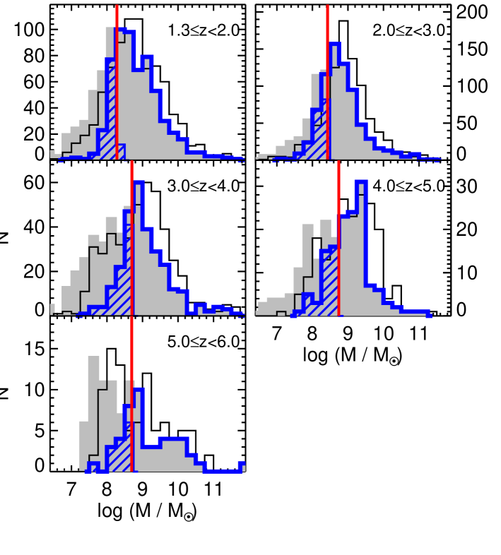
Figure 1.— Stellar mass distribution for the $H<27.5$ sample in the four cluster fields in different redshift bins. The thin black open and grey shaded histograms show the observed and demagnified stellar mass distributions, respectively. The vertical red line shows the mass at which the sample is 90% complete (see text). The thick blue open histograms represent the sample used in the analysis, with the hatched parts showing the galaxies recovered thanks to gravitational lensing. These galaxies have stellar mass below the mass limit, but were included in the sample as their observed mass has been amplified above the threshold (see text).

Intrinsic physical parameters were inferred after correcting for the magnification due to gravitational lensing. The procedure adopted to estimate the magnification factor from the shear and mass surface density maps provided by different teams is described in details in Castellano et al. (2016) (see Priewe et al. 2017 and Meneghetti et al. 2016 for references and for a comparison between different models). We adopted the median magnification, thus excluding possible outlier values associated with a particular model. For fields 1 and 2, at variance with the released catalogs, we only adopted the most updated maps available to date (i.e. v3). This results into the adoption of 6, 8, 7 and 7 models, respectively for the four cluster fields. The magnification factor for the entire sample has a median value of 2, but can reach values as high as $\sim$60, as shown in Castellano et al. (2016).

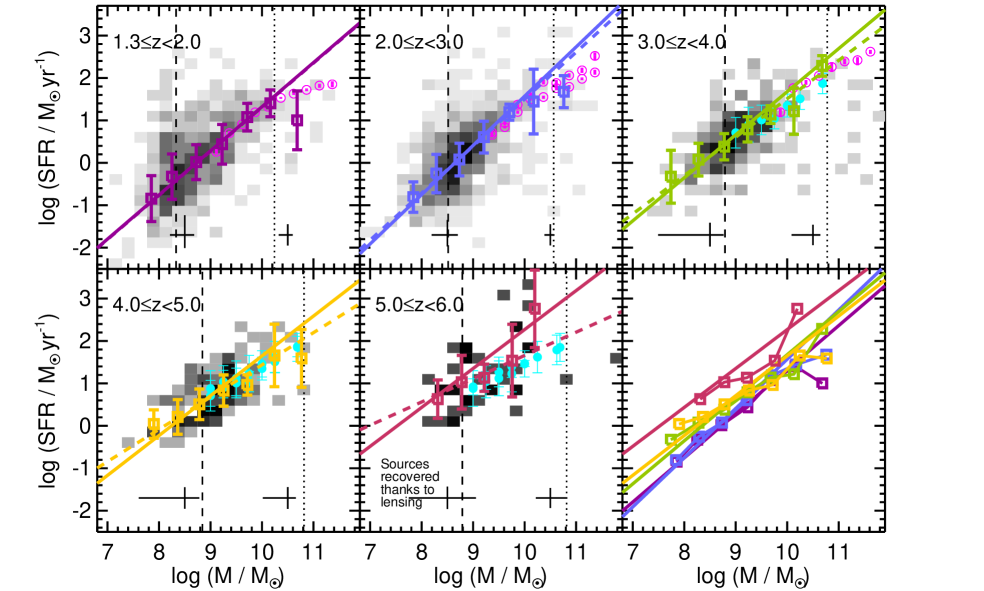
Figure 2.— Relation between the SFR and the stellar mass in different redshift bins. The plane is coloured according to the density of sources, increasing from lightest (0.1% of the total number of sources in that redshift interval) to darkest (6.3%) shades on a linear scale. The open boxes show 2$\sigma$ clipped average values. The dashed coloured lines show the best-fit linear relation obtained with a 2$\sigma$ clipping procedure at stellar masses below the redshift-dependent turnover mass fitted by Tomczak et al. (2016), to avoid the region where the linearity breaks up. The solid coloured lines show the “true” underlying Main Sequence, after correcting for the Eddington bias. At the bottom of each redshift panel, the error bars show the median 1$\sigma$ uncertainties on stellar masses and SFRs for galaxies in the $\log M/$$M_{\odot}$$=$8-9 and 10-11 bins. The dashed vertical lines show the observational mass completeness limit of the sample at the central redshift in each bin: all sources to the left of these lines have been recovered thanks to gravitational lensing. The dotted vertical lines show the turnover mass at the central redshift in each bin as taken from Tomczak et al. (2016). At $z>4$ we adopted the threshold observed at $z=4$. The open magenta and solid cyan circles show the results of Tomczak et al. (2016) and Salmon et al. (2015), respectively. Bottom right panel: Average values and “true” Main Sequence relations in all redshift bins, colour-coded accordingly.

Table 1SFR - Stellar mass relation average values for the cluster Frontier Fields.

$1.3\leq z<2$			$2\leq z<3$			$3\leq z<4$			$4\leq z<5$			$5\leq z<6$
(1)	(2)	(3)	(1)	(2)	(3)	(1)	(2)	(3)	(1)	(2)	(3)	(1)	(2)	(3)
7.85	-0.84	0.54	7.84	-0.81	0.36	7.74	-0.33	0.62	7.90	0.04	0.33	–	–	–
8.25	-0.33	0.53	8.29	-0.25	0.45	8.28	0.07	0.39	8.36	0.21	0.41	8.31	0.63	0.45
8.72	0.02	0.41	8.73	0.08	0.39	8.78	0.38	0.31	8.78	0.51	0.36	8.78	1.03	0.63
9.23	0.44	0.47	9.21	0.61	0.37	9.23	0.79	0.30	9.25	0.83	0.37	9.22	1.13	0.32
9.71	1.08	0.32	9.70	1.19	0.19	9.68	1.14	0.21	9.72	0.96	0.24	9.76	1.54	0.86
10.16	1.40	0.31	10.17	1.44	0.76	10.13	1.22	0.54	10.24	1.66	0.74	10.20	2.76	0.91
10.68	1.00	0.69	10.76	1.68	0.38	10.68	2.28	0.24	10.77	1.59	0.68	–	–	–

Note. — (1): $<$$\log M/$$M_{\odot}$$>$; (2): $<$$\log SFR/$($M_{\odot}$/yr)$>$; (3): $\sigma_{\log SFR}$. Average values and associated scatter have been obtained with a 2$\sigma$ clipping procedure.

Table 2Main Sequence best-fit parameters (corrected for the Eddington bias).

Redshift	$\alpha$	$\beta$
$1.3\leq z<2$	1.04 $\pm$ 0.03	1.01 $\pm$ 0.04
$2\leq z<3$	1.16 $\pm$ 0.03	1.22 $\pm$ 0.03
$3\leq z<4$	1.02 $\pm$ 0.04	1.37 $\pm$ 0.03
$4\leq z<5$	0.94 $\pm$ 0.06	1.37 $\pm$ 0.05
$5\leq z<6$	0.92 $\pm$ 0.15	1.99 $\pm$ 0.13

Note. — Data have been fitted to the functional shape $\log SFR=\alpha\log(M/M_{9.7})+\beta$, where $M_{9.7}=10^{9.7}$$M_{\odot}$, with a 2$\sigma$ clipping procedure.

For studying the MS relation and inferring its slope, it is important to consider a sample that is complete above a given stellar mass. Our sample is selected in the H band, but there is a dispersion in the relation between H band magnitude and stellar mass. Therefore, we assessed the mass completeness limit of our sample by following the procedure outlined in Fontana et al. (2004). Briefly, considering a passively evolving dust-free model, we compute the minimum mass given the magnitude limit of the data and the $M/L$ distribution distribution allowed by the adopted stellar library. Then we use the observed $M/L$ distribution close to the magnitude limit at different redshifts to account for the galaxies that are not observed. We set the mass limit as the mass above which 90% of objects are observed. This redshift-dependent limit is shown as a red vertical line in Fig. 1. However, a fraction of objects intrinsically below the mass limit are actually observed above this threshold thanks to gravitational lensing, boosting the flux from intrinsically fainter, less massive objects. The magnification only depends on the relative position of the lensed and lensing galaxies and not on their physical properties. In particular, it does not depend on their SFR, which will be randomly distributed, in a statistical sense. Based on this argument, we included in our analysis galaxies with intrinsic stellar mass below the mass limit, pushed above the threshold by gravitational lensing magnification. Fig. 1 shows how gravitational lensing allows us to extend the analysis up to a factor of $\sim$10 below the strict observational mass limit (hatched region of the final mass distribution represented by the blue histogram).

After excluding 17 objects at $z>3$ which have been a-posteriori visually inspected due to their suspect very high SFR with respect to the MS, and which turned out to have bad fits due to very noisy photometry, the final sample includes 1711 sources in the redshift range $1.3\leq z<6$.

III. The Main Sequence relation

III.1. Observed Main Sequence

We show in Fig. 2 the relation between SFR and stellar mass, i.e., the MS, in different redshift bins, from $z$$=$1.3 to $z$$=$6. By means of a 2$\sigma$-clipping analysis, we compute average values in bins of stellar mass (reported in Table 1). We recover the mass turnover at high masses, at least out to $z$$=$3, while above this value the turnover moves to higher masses where we lack the required statistics due to the small sky area covered. At the opposite tail, we observe an extension of the MS relation down to stellar masses only rarely probed in previous studies.

In the bottom right panel of Fig. 2 we report the average SFR values in bins of stellar mass at different redshifts. We observe an overall mild increase in the normalisation with redshift and a mild flattening of the slope (at least out to $z\sim 5$, although we note that the highest redshift bin is noisier as it includes fainter sources and is more affected by poor number statistics).

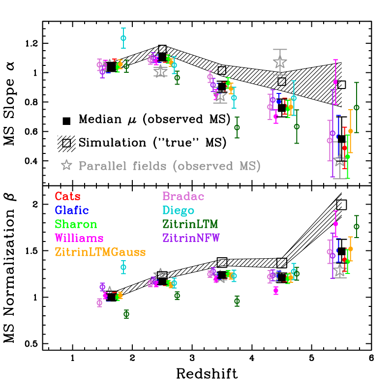
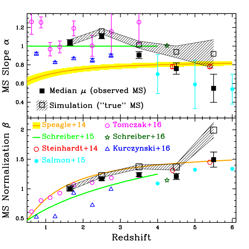
Figure 3.— Evolution of the slope (top panels) and normalization at $\log M/M_{\sun}=9.7$ (bottom panels) of the Main Sequence. In both left and right panels, solid black squares show the observed MS parameters (computed adopting median magnification corrections), while open black squares and the hatched region show the MS parameters and associated 1$\sigma$ uncertainties after correction for the Eddington bias (“true” MS). Left panel: Coloured circles represent the observed MS parameters obtained using the different lensing models, as indicated by the legend in the bottom panel. Open coloured circles refer to lensing models that are not available for all fields: only the fields for which the relevant model was available have been used in these cases. As a consequence, these models show a larger dispersion due to the decreased statistics (the results according to the ‘Diego’ model, only available for field 2, have not been plotted in the highest redshift bin due to poor number statistics). For reference, the MS parameters obtained for the four parallel fields are also shown as grey open stars. The symbols are slightly shifted around the central redshift in each bin for visualization purposes. Right panel: Comparison with MS parameters inferred by previous works, according to the legend in the bottom panel. Normalizations have been rescaled to $\log M/M_{\sun}=9.7$, and the associated error bars have not been shown since they depend on the choice of the mass at which the MS is normalized.

We fit our entire sample (not just the average values) with the linear relation

$$\log SFR=\alpha\log(M/M_{9.7})+\beta$$ (1)

where $M_{9.7}=10^{9.7}$$M_{\odot}$, avoiding the high-mass region where the linearity breaks up. To determine this threshold we used the redshift-dependent best-fit turnover mass obtained by Tomczak et al. (2016) and its value at $z=4$ for higher redshift. We adopt a 2$\sigma$-clipping procedure to remove the outliers: we iteratively reject all points more than 2$\sigma$ apart from the best-fit, where $\sigma$ is calculated as the standard deviation of the residuals. The best-fits are shown as dashed curves in Fig. 2. The evolution of the MS slope and normalization is shown in Fig. 3 (black solid boxes). To verify the robustness of our results against details associated with the magnification correction, in the left panel of Fig. 3 we also show the best-fit MS parameters obtained with each individual lensing model instead of the median magnification. The global picture is unaffected, and the scatter among the various results can be regarded as a measure of the observational uncertainty on the MS parameterization to be associated with lensing modelling. To further confirm that our results are not driven by uncertainties in the magnification corrections, we also compare the MS parameters with those obtained from the parallel fields, where the magnification is very modest.

Overall, we apparently observe a decline in the slope from $\sim 1$ at $z<3$ to $\sim 0.6$ at $z\sim 6$, associated with an increase in the normalization across the entire redshift range studied.

III.2. Correction of the Eddington bias

Since measurement errors in the physical parameters can be high, especially for high redshift faint sources, we tried to take into account their influence on the inferred MS relation. In other words, we correct here the fitted MS for the Eddington bias, that is, we try to recover the intrinsic, “true” MS, that, once convolved with measurement errors, gives rise to the observed relation.

We run a Monte Carlo simulation comprising the following steps:

• Starting from an arbitrary MS, we populate the relation with a realistic logN-logS distribution and a given Gaussian scatter. To this aim, we start from the initial observed sample without applying any magnitude or mass cut. To increase the statistics we replicated the observed distribution 100 times. Given the observed redshift and stellar mass, we assign to each source the SFR predicted by the MS, starting from the observed relation and the observed scatter (the latter is plotted as a black line in Fig. 4). For stellar masses lower than $\log M/$$M_{\odot}$$=$8 and larger than $\log M/$$M_{\odot}$$=$10.3, where our measurement of the scatter is affected by poor number statistics, we adopt a standard value of 0.3 dex.

• We randomly perturb each source in stellar mass and SFR adding Gaussian noise based on the 1$\sigma$ uncertainties on these parameters associated with each object.

• We fit the resulting sample using exactly the same method adopted on real data, i.e., applying the magnitude and mass cuts and adopting a 2$\sigma$-clipping procedure to infer the MS.

• We iteratively modify the input MS, both in slope and normalization, until the best-fit simulated relation matches the observed MS within a tolerance of 0.02 in both parameters. Similarly, we modify the input scatter until the simulated scatter is consistent the observed one. At $\log M/M_{\sun}$$<$8 and $\log M/M_{\sun}$$>$10.3 we assume an input scatter equal to the scatter in the 8$<$$\log M/M_{\sun}$$<$8.8 and 9.6$<$$\log M/M_{\sun}$$<$10.3 mass bins, respectively, since our data prevent us to reliably evaluate the scatter outside this mass range.

• We iterate the procedure 100 times. The resulting parameters and associated uncertainties of the “true” MS as well as its scatter in bins of stellar mass are obtained by computing the average and standard deviation of the best-fit values and of the standard deviation of log(SFR) over the 100 iterations.

The “true” MS are plotted as solid lines in Fig. 2. The best-fit parameters are reported in Table 2, where the uncertainties have been obtained by adding in quadrature the uncertainties on the “true” MS with those on the observed MS. The evolution of the “true” MS is shown by the hatched region in Fig. 3. Once corrected for the Eddington bias, the slope of the MS is consistent with unity across the 1.3–6 redshift range, while the normalization increases with redshift.

The Eddington bias has a negligible effect at $z\lesssim 3$, but it is responsible for a flattening of the relation at higher redshift. It is therefore crucial to take into account the effect of measure uncertainties to reliably estimate the slope of the MS.

III.3. Comparison with previous works

As first step, we compare our results with the analysis of Tomczak et al. (2016), who measured the SFR by stacking on far-infrared images. As shown in Fig. 2, we find excellent agreement despite the completely different approach to estimate the SFR, both concerning the slope and normalization of the relation as well as the turnover at high masses. This agreement corroborates the use of dust-corrected UV luminosity as a SFR tracer for the overall population.

At $z>3$ we compare our MS relations with those of Salmon et al. (2015), based on the CANDELS survey, and once again the agreement is very good (Fig. 2), especially as far as the observed flattening at high-$z$ is concerned. Compared to CANDELS results, we managed, by exploiting gravitational lensing, to extend the analysis to stellar masses more than a factor of 10 lower, probing galaxies with $\log M/$$M_{\odot}$$\sim 7.5$ at $z\lesssim 4$ and $\log M/$$M_{\odot}$$\sim 8$ at higher redshifts.

We also compared our results with the deep analysis of Sawicki (2012). They reach stellar masses as low as $10^{8}$$M_{\odot}$ at $z\sim 2.2$, although their sample is based on a UV-selection and is slightly less complete towards dusty objects (in comparison, our sample is $\sim 1.5$ magnitudes deeper in the UV and includes a few percent of source with E(B-V)$>$0.5). They find a comparable normalization and a flatter slope ($0.89\pm 0.03$).

Another work of almost similar depth as ours is the analysis of Kurczynski et al. (2016), based on HUDF data. They reach stellar masses of $10^{7}$ $M_{\odot}$  at $z<2$ and $10^{8}$ $M_{\odot}$  at $2<z<3$. They find roughly constant slopes around 0.85-0.9 and increasing normalization with decreasing cosmic times, both slightly lower than ours at comparable redshifts.

We show in the right panel of Fig. 3 a comparison of the MS parameters reported by this work with those inferred by some of the most recent studies as well as with the parameterization published by Speagle et al. (2014) and based on a rich compilation of literature results. While there is a general consensus regarding an increasing normalization with redshift (e.g., Santini et al., 2009; Speagle et al., 2014; Schreiber et al., 2015; Tasca et al., 2015; Salmon et al., 2015; Lee et al., 2015; Tomczak et al., 2016), the slope is more uncertain and highly dependent on the details of the analysis, on the SFR tracer adopted and on the sample selection (Santini et al., 2009; Rodighiero et al., 2014; Speagle et al., 2014), as well as, as we showed, on observational uncertainties. Unevolving, approximately linear slopes, as found by our analysis, are reported by the majority of studies cited few lines above, especially at $z\lesssim 4$, while the high redshift work of Salmon et al. (2015) based on CANDELS data reports shallower slopes, ranging from $0.70\pm 0.21$ at $z\sim 4$ to $0.54\pm 0.16$ at $z\sim 6$: their shallower slopes are probably a consequence of the effect of observational uncertainties, that we have corrected thanks to the simulation described in the Sect. III.2.

IV. The scatter around the Main Sequence

The existence of a relation on the SFR–stellar mass diagram as been interpreted as evidence that galaxy growth is likely regulated by cold gas accretion from the IGM on long timescales (e.g. Dekel et al., 2009). In this scenario, the tightness of the MS is related to the level of similarity of the gas accretion histories (see e.g. Shimakawa et al., 2017). It is interesting to investigate whether the scatter around the MS depends on the stellar mass.

The observed scatter around the MS is computed as the standard deviation of log(SFR) after a 2$\sigma$-clipping procedure to remove the MS outliers, and it is shown by the black lines in Fig. 4 as a function of the stellar mass (we do not show the highest redshift bin due to the higher noise level and poorer statistics, which make it difficult to accurately evaluate the scatter). If we focus on the common mass range (9$\lesssim$log$M/$$M_{\odot}$$\lesssim$10), the observed scatter is comparable with that measured by previous works (e.g. Salmon et al., 2015; Schreiber et al., 2015).

The intrinsic scatter around the MS is smaller than the observed one, as the true scatter is convolved with the MS evolution within each bin as well as with the scatter arising from uncertainties in deriving the redshift and the physical parameters (Speagle et al., 2014). To account for the effect of observational uncertainties, we consider the scatter assumed as input to the simulation described in Sect. III.2 (blue stars and lines in Fig. 4), such that the simulated scatter (red circles) matches the observed one. This can be regarded as the intrinsic scatter, except for the fact that it is convolved with the evolution of the MS within each redshift bin. In two of the redshift-mass bins the simulated scatter turns out to be significantly larger than the observed one even by assuming no intrinsic scatter in the simulation. This suggests that the large observational uncertainties completely dominate the scatter of the data points around the MS and/or the simplified assumptions in our simulation (e.g. the assumption of Gaussian noise) hamper the evaluation of the intrinsic scatter in these bins.

Overall however, we observe an indication, although not very robust, that the intrinsic scatter decreases with the stellar mass, although this trend seems to be reversed (or is impossible to evaluate, as discussed above) at $3<z<4$. This tentative trend is in contrast with recent studies reporting no dependency on the stellar mass (Whitaker et al., 2012; Schreiber et al., 2015; Salmon et al., 2015; Kurczynski et al., 2016), although not extending to masses lower than $10^{9}$$M_{\odot}$(except for the latter study). It instead agrees with the results of Salim et al. (2007), who finds that in the local Universe the scatter declines by 0.11 dex per order of magnitude in stellar mass from $10^{8}$ to $10^{10.5}$$M_{\odot}$.

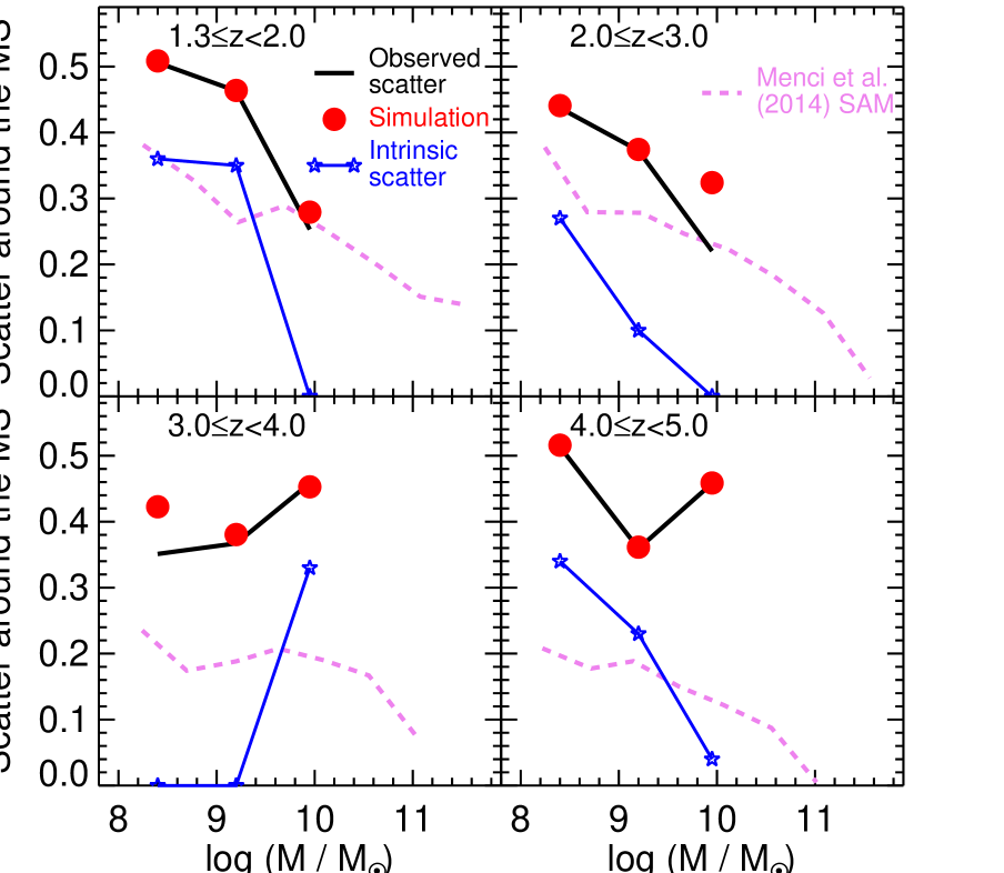
Figure 4.— Scatter around the MS as a function of stellar mass, in different redshift bins. The black lines show the observed scatter, i.e. the standard deviation of log(SFR), as inferred through a 2$\sigma$-clipping procedure. The red circles are the scatter computed from the simulation, using the same technique. Blue stars connected by blue lines show the intrinsic scatter, i.e. the scatter assumed as input in the simulation such that the output simulated scatter matches the observed one. Dashed pink lines are the predictions of the hierarchical model of galaxy formation of Menci et al. (2014), where the scatter has been computed with the same technique adopted on the data.

An increase in the scatter around the MS at low stellar masses as well as low redshift is a natural outcome of theoretical models of galaxy formation, and arises from the hierarchical structure formation and/or from the highly efficient stellar feedback processes in small halos (e.g. Merlin et al., 2012; Lamastra et al., 2013; Hopkins et al., 2014). To visualize this effect, we plot in Fig. 4 the predictions of the semi-analytical model of Menci et al. (2014), which, not surprisingly, forecasts a smaller scatter than the observations as it is not affected by measurement errors. In a hierarchical scenario, high mass galaxies have a large number of progenitors already collapsed at high-$z$, as they formed in high density regions of the primordial dark matter density field. The SFHs of these progenitor galaxies are peaked at high redshift since the gas cooling and the star formation efficiency are extremely efficient at early epochs. In addition, due to the higher compactness and lower virial temperatures of high-$z$ dark matter halos, supernova feedback is less efficient at heating/expelling the gas from the galaxy. Conversely, the smaller number of progenitors of low mass galaxies, and their different collapse time allowing also more prolonged star formation activity, lead to a larger variety of their SFHs.

V. The evolution of the specific SFR

We investigate here the evolution of the average, or typical, specific SFR, i.e. the SFR per unit stellar mass (sSFR=SFR/$M$), which captures information on the mass build-up process across cosmic time. Indeed, theoretical models in which galaxy growth is dominated by cold accretion predict that the sSFR should increase with redshift as $(1+z)^{2.25}$ (e.g. Dekel et al., 2009; Davé et al., 2011a).

Since the sSFR is not constant with the stellar mass (i.e. the slope of the MS is not unitary at all redshifts), we derived the average sSFR at constant stellar mass. We considered the $\log M/$$M_{\odot}$$=9.5-10$ mass bin (average value $<\log M/$$M_{\odot}$$>\sim 9.7$). Despite adopting a fixed stellar mass at all redshifts implies considering a different galaxy population at different times, this allows an easy comparison with previous results computed at the reference mass of $\log M/$$M_{\odot}$$=9.7$, and allows us to extend the analysis of the evolution of the sSFR outside the redshift range probed by the present work (i.e. at $z<1.3$ and $z>6$). We computed the observed average values by means of a 2$\sigma$-clipping procedure directly on the galaxies in this mass bin, without using the best-fit MS relation (black solid squares). Given that the MS slope at high-$z$ is sometimes found to be (slightly) sub-linear, the sSFR is a decreasing function of the stellar mass. Not to run the risk of underestimating the average sSFR, it is therefore essential to ensure completeness at the chosen mass bin. The chosen mass bin is well above the completeness level in our data. Finally, to take into account the effect of observational uncertainties, we make use of the Eddington-corrected MS estimated from the simulation (Sect. III.2) and compute the typical sSFR at $\log M/$$M_{\odot}$$=9.7$ (black open squares). We adopt the same procedure for the data from the literature when the average value is not available at the relevant mass.

Our results are in line with the compilation of data from previous works (see Fig. 5). Until a few years ago, observations appeared to show that the sSFR increased steeply from $z\sim 0$ to $z\sim 2$ (e.g. Noeske et al., 2007; Santini et al., 2009; Karim et al., 2011) and flattened at higher redshift (e.g. Stark et al., 2009; González et al., 2010; Reddy et al., 2012; González et al., 2010; Labbé et al., 2010; McLure et al., 2011), in sharp contrast with theoretical predictions (see e.g. Weinmann et al., 2011). The improvement in the dust-correction estimates and the inclusion of nebular lines in SED modelling have led to higher sSFR estimates at high redshift, alleviating the tension with theoretical models. A moderate increase in the sSFR compared to its value at $z\sim 2$ is now found in many studies (Stark et al., 2013; González et al., 2014; Tasca et al., 2015; Mármol-Queraltó et al., 2016; Koprowski et al., 2016), especially at $z\gtrsim 5$. Nevertheless, the evolution seems overall milder than that expected in an accretion-dominated scenario, although some results are getting closer (de Barros et al., 2014; Faisst et al., 2016). We note, however, that given the scatter in the MS, a flat trend cannot be ruled out.

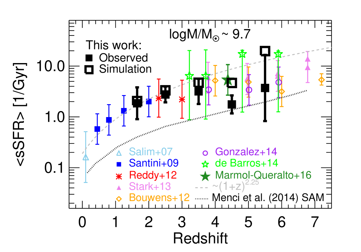
Figure 5.— Evolution of the average sSFR as a function of redshift for $\log M/$$M_{\odot}$$\sim 9.7$ galaxies. Error bars show the standard deviation of log sSFR, computed with a 2-$\sigma$ clipping procedure. Black squares are the results of this work: solid symbols are the observed values in the $\log M/$$M_{\odot}$$\sim 9.5-10$ mass bin, open ones are the result of the simulation, computed from the corrected MS at $\log M/$$M_{\odot}$$=9.7$. The other symbols present results from the literature according to the legend. When the average sSFR was not available at the chosen mass (as for Santini et al. 2009 and Salim et al. 2007), we computed it by means of the best-fit MS relations. As for the results of Mármol-Queraltó et al. (2016), we only considered their 3.8-5.0 redshift bin, whose median stellar mass is equal to $\log M/$$M_{\odot}$$\sim 9.7$, and we adopted a scatter of 0.3 dex. The black dotted line is the prediction of the semi-analytical model of galaxy formation of Menci et al. (2014) in the $\log M/$$M_{\odot}$$\sim 9.5-10$ mass bin. The dashed gray curve shows the prediction of accretion-dominated models (e.g. Dekel et al., 2009), normalized to the bulk of data points at $z\sim 2$. We note that the dip shown by our observed values at $z\sim 4.5$ is explained by the average lower SFR compared to the MS relation around the reference stellar mass because of poor number statistics (Fig. 2).

We observe an evolution by a factor of $\sim 2$ from $z\sim 5.5$ to $z\sim 1.6$. Although a steeper trend is found when correcting for the Eddington bias, the large scatter associated to the highest redshift bin prevent us from drawing firm conclusions in this regard. The observed decrease is lower than that predicted by theoretical models in the same redshift interval (a factor of $\sim 8$), implying that some sort of star formation suppression at high redshift is required to match the observations (feedback effects can modify the trend, see e.g. Davé et al. 2011b), that the effect of metallicity should be taken into account (Krumholz & Dekel, 2012) and that other processes besides pure accretion are at play in assembling galaxies, such as mergers (e.g. Tasca et al., 2015; Faisst et al., 2016). The evolution of the sSFR is a critical observable to understand all these processes regulating star formation and galaxy growth. We note that a tension between observations and theoretical models is also observed in terms of absolute values of the sSFR (see the predictions of Menci et al. 2014 semi-analytical model). This effect is closely connected with the well-known overall lower normalization of the predicted MS compared to the observed one (e.g. Santini et al., 2009; Lamastra et al., 2013).

VI. Summary

We have studied the Main Sequence relation of star forming galaxies, i.e., the relation between galaxy SFR and stellar mass, in the first four HST Frontier Fields. Thanks to gravitational lensing amplification of faint sources from massive foreground galaxy clusters, we could extend the analysis to masses lower than has usually been possible with the deepest data available before the Frontier Fields program and a factor of $\sim$10 lower than most studies. We investigated the redshift range $1.3\leq z<6$ and probed stellar masses down to $\log M/$$M_{\odot}$$\sim 7.5$ at $z\lesssim 4$ and $\log M/$$M_{\odot}$$\sim 8$ at higher redshifts. We find that the MS relation extends to such low masses. At the opposite side, we recover the mass turnover at high masses at $z<3$, i.e., where we have enough statistics at $\log M/$$M_{\odot}$$\gtrsim 10.5$. We run an accurate Montecarlo simulation to take into account the effect of measure uncertainties on stellar masses and SFRs and correct for the Eddington bias. Such step is crucial to reliably measure the slope of the MS, which tends to be flattened by observational errors at $z\gtrsim 3$. We find increasing normalizations with redshift and an approximately linear unevolving slope.

The combination of deep HST observations and gravitational lensing allows us to observe tentative evidence that the scatter around the MS relation increases at low stellar masses, although we cannot make a strong claim. If verified, this result implies a higher level of uniformity in the SFHs at high masses, in agreement with observations in the local Universe and with the predictions of theoretical models of galaxy evolution.

We confirm the previously observed mild increase in the average sSFR from $z\sim 1.6$ to $z\sim 5.5$ by a factor of $\sim$2, in tension with the steeper trend predicted by accretion-driven models (a factor of $\sim 8$ in the same redshift interval). Being able to reproduce the evolution of the sSFR is crucial to understand the processes regulating the star formation and galaxy growth at different cosmic epochs and assessing the relative importance of gas accretion versus merging as well as the role of feedback mechanisms.

JWST observations in the next future will allow to extend the analysis of the MS to even lower masses. Discerning between a MS that keeps extending to faint sources and a broken relation will provide hints on physical mechanisms such as feedback and reionization, or cold vs warm dark matter scenarios.

References

- Bertin & Arnouts (1996) Bertin, E., & Arnouts, S. 1996, A&AS, 117, 393
- Bouwens et al. (2016) Bouwens, R., Aravena, M., Decarli, R., et al. 2016, ArXiv: 1606.05280, arXiv:1606.05280
- Brinchmann et al. (2004) Brinchmann, J., Charlot, S., White, S. D. M., et al. 2004, MNRAS, 351, 1151
- Bruzual & Charlot (2003) Bruzual, G., & Charlot, S. 2003, MNRAS, 344, 1000
- Calzetti et al. (2000) Calzetti, D., Armus, L., Bohlin, R. C., et al. 2000, ApJ, 533, 682
- Capak et al. (2015) Capak, P. L., Carilli, C., Jones, G., et al. 2015, Nature, 522, 455
- Castellano et al. (2012) Castellano, M., Fontana, A., Grazian, A., et al. 2012, A&A, 540, A39
- Castellano et al. (2014) Castellano, M., Sommariva, V., Fontana, A., et al. 2014, A&A, 566, A19
- Castellano et al. (2016) Castellano, M., Amorín, R., Merlin, E., et al. 2016, A&A, 590, A31
- Cullen et al. (2017) Cullen, F., McLure, R. J., Khochfar, S., Dunlop, J. S., & Dalla Vecchia, C. 2017, ArXiv e-prints, arXiv:1701.07869
- Daddi et al. (2007) Daddi, E., Dickinson, M., Morrison, G., et al. 2007, ApJ, 670, 156
- Daddi et al. (2010) Daddi, E., Elbaz, D., Walter, F., et al. 2010, ApJ, 714, L118
- Dahlen et al. (2013) Dahlen, T., Mobasher, B., Faber, S. M., et al. 2013, ApJ, 775, 93
- Davé et al. (2011a) Davé, R., Finlator, K., & Oppenheimer, B. D. 2011a, MNRAS, 416, 1354
- Davé et al. (2011b) Davé, R., Oppenheimer, B. D., & Finlator, K. 2011b, MNRAS, 415, 11
- de Barros et al. (2014) de Barros, S., Schaerer, D., & Stark, D. P. 2014, A&A, 563, A81
- Dekel et al. (2009) Dekel, A., Birnboim, Y., Engel, G., et al. 2009, Nature, 457, 451
- Di Criscienzo et al. (2017) Di Criscienzo, M., Merlin, E., Castellano, S., et al. 2017, A&A, submitted
- Dunlop et al. (2017) Dunlop, J. S., McLure, R. J., Biggs, A. D., et al. 2017, MNRAS, 466, 861
- Elbaz et al. (2007) Elbaz, D., Daddi, E., Le Borgne, D., et al. 2007, A&A, 468, 33
- Elbaz et al. (2011) Elbaz, D., Dickinson, M., Hwang, H. S., et al. 2011, A&A, 533, A119
- Faisst et al. (2016) Faisst, A. L., Capak, P., Hsieh, B. C., et al. 2016, ApJ, 821, 122
- Fontana et al. (2004) Fontana, A., Pozzetti, L., Donnarumma, I., et al. 2004, Astronomy & Astrophysics, 424, 23
- Fudamoto et al. (2017) Fudamoto, Y., Oesch, P. A., Schinnerer, E., et al. 2017, ArXiv e-prints, arXiv:1705.01559
- Genzel et al. (2010) Genzel, R., Tacconi, L. J., Gracia-Carpio, J., et al. 2010, MNRAS, 407, 2091
- González et al. (2014) González, V., Bouwens, R., Illingworth, G., et al. 2014, ApJ, 781, 34
- González et al. (2010) González, V., Labbé, I., Bouwens, R. J., et al. 2010, ApJ, 713, 115
- Hopkins et al. (2014) Hopkins, P. F., Kereš, D., Oñorbe, J., et al. 2014, MNRAS, 445, 581
- Karim et al. (2011) Karim, A., Schinnerer, E., Martínez-Sansigre, A., et al. 2011, ApJ, 730, 61
- Kennicutt & Evans (2012) Kennicutt, R. C., & Evans, N. J. 2012, ARA&A, 50, 531
- Koprowski et al. (2016) Koprowski, M. P., Dunlop, J. S., Michałowski, M. J., et al. 2016, MNRAS, 458, 4321
- Krumholz & Dekel (2012) Krumholz, M. R., & Dekel, A. 2012, ApJ, 753, 16
- Kurczynski et al. (2016) Kurczynski, P., Gawiser, E., Acquaviva, V., et al. 2016, ApJ, 820, L1
- Labbé et al. (2010) Labbé, I., González, V., Bouwens, R. J., et al. 2010, ApJ, 716, L103
- Lamastra et al. (2013) Lamastra, A., Menci, N., Fiore, F., & Santini, P. 2013, A&A, 552, A44
- Lee et al. (2015) Lee, N., Sanders, D. B., Casey, C. M., et al. 2015, ApJ, 801, 80
- Lotz et al. (2017) Lotz, J. M., Koekemoer, A., Coe, D., et al. 2017, ApJ, 837, 97
- Magnelli et al. (2014) Magnelli, B., Lutz, D., Saintonge, A., et al. 2014, A&A, 561, A86
- Mancuso et al. (2016) Mancuso, C., Lapi, A., Shi, J., et al. 2016, ApJ, 833, 152
- Mármol-Queraltó et al. (2016) Mármol-Queraltó, E., McLure, R. J., Cullen, F., et al. 2016, MNRAS, 460, 3587
- McLure et al. (2011) McLure, R. J., Dunlop, J. S., de Ravel, L., et al. 2011, MNRAS, 418, 2074
- Menci et al. (2014) Menci, N., Gatti, M., Fiore, F., & Lamastra, A. 2014, A&A, 569, A37
- Meneghetti et al. (2016) Meneghetti, M., Natarajan, P., Coe, D., et al. 2016, ArXiv e-prints, arXiv:1606.04548
- Merlin et al. (2012) Merlin, E., Chiosi, C., Piovan, L., et al. 2012, MNRAS, 427, 1530
- Merlin et al. (2015) Merlin, E., Fontana, A., Ferguson, H. C., et al. 2015, A&A, 582, A15
- Merlin et al. (2016) Merlin, E., Amorín, R., Castellano, M., et al. 2016, A&A, 590, A30
- Meurer et al. (1999) Meurer, G. R., Heckman, T. M., & Calzetti, D. 1999, ApJ, 521, 64
- Michałowski et al. (2012) Michałowski, M. J., Dunlop, J. S., Cirasuolo, M., et al. 2012, A&A, 541, A85
- Michałowski et al. (2014) Michałowski, M. J., Hayward, C. C., Dunlop, J. S., et al. 2014, A&A, 571, A75
- Narayanan et al. (2012) Narayanan, D., Krumholz, M. R., Ostriker, E. C., & Hernquist, L. 2012, MNRAS, 421, 3127
- Noeske et al. (2007) Noeske, K. G., Weiner, B. J., Faber, S. M., et al. 2007, ApJ, 660, L43
- Peng et al. (2010) Peng, Y.-j., Lilly, S. J., Kovač, K., et al. 2010, ApJ, 721, 193
- Prevot et al. (1984) Prevot, M. L., Lequeux, J., Prevot, L., Maurice, E., & Rocca-Volmerange, B. 1984, A&A, 132, 389
- Priewe et al. (2017) Priewe, J., Williams, L. L. R., Liesenborgs, J., Coe, D., & Rodney, S. A. 2017, MNRAS, 465, 1030
- Reddy et al. (2012) Reddy, N. A., Pettini, M., Steidel, C. C., et al. 2012, ApJ, 754, 25
- Renzini & Peng (2015) Renzini, A., & Peng, Y.-j. 2015, ApJ, 801, L29
- Rodighiero et al. (2011) Rodighiero, G., Daddi, E., Baronchelli, I., et al. 2011, ApJ, 739, L40
- Rodighiero et al. (2014) Rodighiero, G., Renzini, A., Daddi, E., et al. 2014, MNRAS, 443, 19
- Salim et al. (2007) Salim, S., Rich, R. M., Charlot, S., et al. 2007, ApJS, 173, 267
- Salmon et al. (2015) Salmon, B., Papovich, C., Long, J., et al. 2015, ArXiv e-prints, arXiv:1512.05396
- Salpeter (1955) Salpeter, E. E. 1955, ApJ, 121, 161
- Santini et al. (2009) Santini, P., Fontana, A., Grazian, A., et al. 2009, A&A, 504, 751
- Santini et al. (2014) Santini, P., Maiolino, R., Magnelli, B., et al. 2014, A&A, 562, A30
- Santini et al. (2015) Santini, P., Ferguson, H. C., Fontana, A., et al. 2015, ApJ, 801, 97
- Sargent et al. (2012) Sargent, M. T., Béthermin, M., Daddi, E., & Elbaz, D. 2012, ApJ, 747, L31
- Sawicki (2012) Sawicki, M. 2012, MNRAS, 421, 2187
- Schaerer & de Barros (2009) Schaerer, D., & de Barros, S. 2009, A&A, 502, 423
- Schreiber et al. (2015) Schreiber, C., Pannella, M., Elbaz, D., et al. 2015, A&A, 575, A74
- Scoville et al. (2015) Scoville, N., Faisst, A., Capak, P., et al. 2015, ApJ, 800, 108
- Shimakawa et al. (2017) Shimakawa, R., Koyama, Y., Prochaska, J. X., et al. 2017, ArXiv e-prints, arXiv:1705.01127
- Speagle et al. (2014) Speagle, J. S., Steinhardt, C. L., Capak, P. L., & Silverman, J. D. 2014, ApJS, 214, 15
- Stark et al. (2009) Stark, D. P., Ellis, R. S., Bunker, A., et al. 2009, ApJ, 697, 1493
- Stark et al. (2013) Stark, D. P., Schenker, M. A., Ellis, R., et al. 2013, ApJ, 763, 129
- Steinhardt et al. (2014) Steinhardt, C. L., Speagle, J. S., Capak, P., et al. 2014, ApJ, 791, L25
- Tasca et al. (2015) Tasca, L. A. M., Le Fèvre, O., Hathi, N. P., et al. 2015, A&A, 581, A54
- Tomczak et al. (2016) Tomczak, A. R., Quadri, R. F., Tran, K.-V. H., et al. 2016, ApJ, 817, 118
- Weinmann et al. (2011) Weinmann, S. M., Neistein, E., & Dekel, A. 2011, MNRAS, 417, 2737
- Whitaker et al. (2012) Whitaker, K. E., van Dokkum, P. G., Brammer, G., & Franx, M. 2012, ApJ, 754, L29
- Whitaker et al. (2014) Whitaker, K. E., Franx, M., Leja, J., et al. 2014, ApJ, 795, 104
- Whitaker et al. (2015) Whitaker, K. E., Franx, M., Bezanson, R., et al. 2015, ApJ, 811, L12