GMC Collisions As Triggers of Star Formation. IV.
The Role of Ambipolar Diffusion

Abstract

We investigate the role of ambipolar diffusion (AD) in collisions between magnetized giant molecular clouds (GMCs), which may be an important mechanism for triggering star cluster formation. Three dimensional simulations of GMC collisions are performed using a version of the Enzo magnetohydrodynamics code that has been extended to include AD. The resistivities are calculated using the 31-species chemical model of Wu et al. (2015). We find that in the weak-field, $10\>{\rm\mu G}$ case, AD has only a modest effect on the dynamical evolution during the collision. However, for the stronger-field, $30\>{\rm\mu G}$ case involving near-critical clouds, AD results in formation of dense cores in regions where collapse is otherwise inhibited. The overall efficiency of formation of cores with $n_{\rm H}\geq 10^{6}\>{\rm cm}^{-3}$ in these simulations is increases from about 0.2% to 2% once AD is included, comparable to observed values in star-forming GMCs. The gas around these cores typically has relatively slow infall at speeds that are a modest fraction of the free-fall speed.

1 Introduction

Collisions between giant molecular clouds (GMCs) have been proposed as a mechanism to initiate the conditions necessary for gas to form massive stars and star clusters (e.g., Scoville et al. 1986; Tan 2000). These conditions are expected to involve there being a large mass of dense gas in gravitationally unstable clumps and cores, e.g., as potentially traced by Infrared Dark Clouds (IRDCs) (see, e.g., Tan et al. 2014). Magnetic fields could play an important role in this process, especially if they inhibit collapse and regulate the star formation rate (SFR) in GMCs during the normal circumstances when they are not colliding (e.g., McKee 1989; Li et al. 2014). Average SFRs in GMCs are known to be very inefficient per local free-fall time (Zuckerman & Evans, 1974; Krumholz & Tan, 2007), but to also show large variation (Lee et al., 2016), which could be caused by triggering by cloud collisions.

During the process of collapse from low density gas conditions to dense cores and protostars, the mass-to-magnetic flux ratio increases by many orders of magnitude and a threshold must be crossed of gas initially being magnetically subcritical (i.e., $B$-fields are strong enough to resist collapse) to being magnetically super-critical ($B$-fields are not strong enough to stop collapse). The imperfect coupling between the gas and the magnetic field leads to ambipolar diffusion (or ion-neutral drift) (Mestel & Spitzer, 1956), which is one way to allow for collapse to be accelerated, especially in situations where strong field gradients are created such as a cloud-cloud collision.

Magnetic field strengths within the diffuse interstellar medium (ISM) have been measured via the Zeeman effect with values of $6\pm 1.8\,{\rm\mu G}$ (Heiles & Troland, 2005) over a wide range of observed column densities. The magnetic field strength remains roughly independent of gas density until a threshold density, $n_{\rm H}\sim 300\,\,{\rm cm}^{-3}$, is reached, after which it begins to increase with gas density as $B\propto\rho^{\kappa}$ with $\kappa\simeq 0.65$ (Crutcher, 1999; Falgarone et al., 2008; Crutcher et al., 2010). This increase can be interpreted as being due to flux freezing in the collapse of spherical, weakly-magnetized clouds (Mestel, 1966). Such a dependence of $B$-field strength with density has also been seen in the simulations of self-gravitating turbulence of, e.g., Li et al. (2015) and Mocz et al. (2017). In more strongly magnetized clouds, i.e., with Alfvén Mach numbers $\lesssim 1$, a shallower relation, with $\kappa\simeq 0.5$ is expected (Tritsis et al., 2015; Mocz et al., 2017) and Tritsis et al. (2015) have also argued that such a value of $\kappa$ is a better match to the observational data.

Concerning the collapse of GMCs, clumps and massive cores, since typical temperatures are $\sim 15\,{\rm K}$, thermal pressure alone is incapable of providing significant support against gravity. Both magnetic fields and turbulence are in principle capable of supporting the clouds, if sufficiently strong. The degree of support provided by the magnetic field is measured by the mass-to-flux ratio $\mu$,

$$\mu=\frac{M/\Phi}{1/\sqrt{63G}},$$ (1)

where $M$ is the cloud mass and $\Phi$ is the magnetic flux through the cloud. Here $\mu$ has been normalized to the critical value, so that $\mu<1$ is the condition for stability against collapse in the limit of ideal MHD (Mouschovias & Spitzer, 1976). In the case of initially subcritical clouds, ambipolar diffusion allows gas to be redistributed across flux tubes, creating structures that are locally supercritical and unstable. For sufficiently supercritical clouds, ambipolar diffusion is not requisite for collapse to occur, especially if large magnetic field and/or velocity gradients are created in the cloud. One mechanism that may induce such gradients is GMC collisions.

Observationally, inferring the mass-to-flux ratio in interstellar clouds is difficult due to projection effects associated with measuring the magnetic field and the column density along the field line. Crutcher et al. (2009) attempted to measure the change in the projected mass-to-flux ratio between cores and their surrounding envelopes and concluded that the mass-to-flux ratio decreases from the envelope to core. An increase in the mass-to-flux ratio from the envelope to the core is expected to be a sign of ambipolar diffusion acting in subcritical clouds, a result not favored by the Crutcher et al. (2009) analysis. However, Mouschovias & Tassis (2009, 2010) have called into question the validity of the conclusions on statistical grounds (but, see also Li et al. 2015).

Li & Houde (2008) proposed that the action of ambipolar diffusion could be inferred through the differing velocity dispersions observed for spatially coincident ions and neutrals. At scales above the ambipolar diffusion dissipation scale, the ions and neutrals are expected to remain well-coupled, resulting in near-identical power spectra for the two species. Below the dissipation scale, however, ion modes are quickly damped while the neutrals experience negligible drag due to the ions. While it may not be feasible to observe the dissipation scale directly, the velocity dispersion retains information about all scales smaller than the beam size. The technique has been applied multiple times with the resulting dissipation scales being on the order of $10^{-3}$ to $10^{-2}\,{\rm pc}$ (Li et al., 2010; Hezareh et al., 2010, 2014).

In this paper we investigate the role ambipolar diffusion plays during the process of GMC-GMC collisions. Wu et al. (2015, hereafter Paper I) and Wu et al. (2017b, hereafter Paper II) investigated how such collisions can trigger dense clump formation, including magnetic fields treated under the assumption of ideal magneto-hydrodynamics (MHD) and a model of the multiphase interstellar medium. In Wu et al. (2017a, hereafter Paper III), star formation was explicitly included in the simulations with various sub-grid models investigated, including examples in which a mass-to-flux threshold criterion needs to be reached in order for gas in a cell to be able to form stars.

This work expands upon Papers I and II through the inclusion of ambipolar diffusion, modifications to the heating and cooling model, and the expansion to larger effective resolutions. Section 2 describes the numerical model, including the initial conditions (Section 2.1), the treatment of heating and cooling (Section 2.2), the inclusion of ambipolar diffusion (Section 2.3), and the calculation of resistivities (Section 2.4). The results are presented in Section 3 and the conclusions in Section 4. Tests of the ambipolar diffusion module are described in Appendix A.

2 Model of Colliding and Non-Colliding GMCs

The model presented here is very similar to that presented in Paper II, with the differences confined to updates to the heating and cooling model and the inclusion of ambipolar diffusion.

2.1 Initial Conditions

The simulation volume is a $L=128\,{\rm pc}$ sided cube filled with an ambient medium with $n_{\rm H,0}=10\,{\rm cm^{-3}}$. Two identical, spherical GMCs with radii $R_{\rm GMC}=20\,{\rm pc}$ and $n_{\rm H,0}=100\,{\rm cm^{-3}}$ are embedded within the ambient medium and offset with an impact parameter $b=0.5R_{\rm GMC}$. In addition to the hydrogen component, the gas contains heavier species in abundances representative of the local interstellar medium.

Within each model cloud, a turbulent velocity field is initialized with a spectrum $v_{\rm k}^{2}\propto k^{-4}$, where $k$ is the wavenumber. For gas with $T=15\,{\rm K}$, the virial scale Mach number $\mathcal{M}_{s}=\sigma/c_{\rm s}=23$. The $k$-modes are chosen to be in the range $2<k/(\pi/L)<20$. In addition to the turbulent velocity spectrum, the clouds are imparted with a relative velocity $v_{\rm rel}$ with the fiducial value being $v_{\rm rel}=10\,{\rm km\,s^{-1}}$, although we also investigate the stationary (non-colliding) case $v_{\rm rel}=0\,{\rm km\,s^{-1}}$. In the simulation frame of reference, half of the gas is given a velocity of $+v_{\rm rel}/2$, while the other half given a velocity of $-v_{\rm rel}/2$.

A uniform magnetic field with field strength $B=10\,{\rm\mu G}$ or $30\,{\rm\mu G}$ is initialized with a direction at an angle $\theta=60^{\circ}$ relative to the collision axis of the clouds. Ignoring the contribution from the ambient medium and taking the flux through the cloud to be $\Phi=\pi R_{\rm GMC}^{2}B_{0}$, the initial mass-to-flux ratios are $\mu_{0}=3.8$ for the $10\,{\rm\mu G}$ runs and $\mu_{0}=1.3$ for the $30\,{\rm\mu G}$ runs, both supercritical and globally unstable against collapse. Due to their large extents, each cloud may fragment along the field lines, creating objects with smaller, potentially subcritical, mass-to-flux ratios.

Due to the spherical geometry adopted for the model GMCs, the central flux tube is loaded with more mass resulting in a central mass-to-flux ratio, $\mu_{\rm center}$, of

$$\mu_{\rm center}\sim\frac{N/B_{0}}{1/\sqrt{63G}}=\frac{2R_{\rm GMC}\rho_{0}/B_{0}}{1/\sqrt{63G}}=\left\{\begin{matrix}5.7,&B=10\,{\rm\mu G}\\ 1.9,&B=30\,{\rm\mu G}\end{matrix}\right.\,\,.$$ (2)

The larger values of $\mu$ associated with the central flux tubes through the cloud could potentially result in preferential collapse in these regions compared to near the cloud boundaries.

To investigate the role of ambipolar diffusion, identical initial conditions are run with ambipolar diffusion enabled and with ambipolar diffusion disabled (i.e., in the ideal MHD limit).

The top grid resolution is $128^{3}$ with 4 levels of refinement, resulting in the smallest grid size being $\Delta x=0.0625\,{\rm pc}$. Grid refinement is based on the requirement that the Jeans length is resolved with at least 8 zones. While it has been pointed out by Federrath et al. (2011) that a minimum of 30 zones per Jeans length is required to resolve turbulence on the Jeans scale, this is computationally prohibitive given the range of scales in the problem and the quadratic scaling of the ambipolar diffusion timestep with grid size. As the minimum effective grid size is $\Delta x=0.0625\,{\rm pc}$, the collapse of gas on core-scales is unresolved. At the maximum refinement level and for $T=10\,{\rm K}$ molecular gas, the Jeans length is no longer resolved by 8 zones at $3\times 10^{3}\,{\rm cm^{-3}}$, 4 zones at $1.2\times 10^{4}\,{\rm cm^{-3}}$, and 1 zone at $2\times 10^{5}\,{\rm cm^{-3}}$. This should be kept in mind when interpreting details of the collapse of individual cores.

2.2 Heating and Cooling

Heating and cooling are implemented using the Grackle chemistry and cooling library (Smith et al., 2017). The heating and cooling rates are the same as in Wu et al. (2015), although updating to Grackle 2.2 allows for the use of the mean molecular weight generated by the PyPDR and CLOUDY (Ferland et al., 2013) codes. In the previous Grackle 2.1 code, the mean molecular weight was determined by an analytic fit as a function of temperature and was independent of density. While the mean molecular weights in the analytic fit agree with the new tabular values in the cold, dense molecular gas, there is a divergence between the two at higher temperatures and lower gas densities. Additionally, the cooling timestep $\Delta t_{\rm cool}$ is now included in the total dynamical timestep. This ensures that gas does not, through unphysical means, diverge too far from equilibrium temperatures. For numerical expediency, however, a minimum cooling timestep $\Delta t_{\rm cool,min}\sim 600\,{\rm yr}$ is included as the cooling timestep can become prohibitively small at large densities. The cooling timestep takes the form

$$\Delta t_{\rm cool}=\max\left(\frac{0.2\rho e}{|\Gamma-\Lambda|+\epsilon},\Delta t_{\rm cool,min}\right),$$ (3)

where $\rho$ is the gas density, $e$ is the specific internal energy, $\Gamma$ is the volumetric heating rate, $\Lambda$ is the volumetric cooling rate, and the small factor $\epsilon$ is included to avoid divergence at thermal equilibrium. This timestep is used in calculating the dynamical timestep and is independent of the internal subcycling used by the Grackle cooling routine. These changes result in a small difference in the gas temperatures at low densities between results presented in Paper II and those presented here.

2.3 Ambipolar Diffusion

Ambipolar diffusion is included in Enzo’s Dedner MHD solver (Dedner et al., 2002; Wang & Abel, 2009) through the modification of the induction equation to include non-ideal terms:

$$\frac{\partial\boldsymbol{B}}{\partial t}-\boldsymbol{\nabla}\times\left(\boldsymbol{v}\times\boldsymbol{B}\right)=-\boldsymbol{\nabla}\times\left(D_{\rm AD}\left(\boldsymbol{\nabla}\times\boldsymbol{B}\right)\times\boldsymbol{b}\times\boldsymbol{b}\right),$$ (4)

where $D_{\rm AD}=c^{2}\eta_{\rm AD}/4\pi$ is the ambipolar diffusion constant, $\eta_{\rm AD}$ is the resistivity, and $\boldsymbol{b}$ is a unit vector in the direction of $\boldsymbol{B}$. The terms on the right hand side of equation 4 are included as an explicit update in the source term step. To ensure stability, the explicit timestep is limited by the ambipolar diffusion timestep,

$$\Delta t_{\rm AD}=\frac{\delta\min\left(\Delta x^{2},\Delta y^{2},\Delta z^{2}\right)}{D_{\rm AD}},$$ (5)

where $\delta=0.1$ is a safety factor included to ensure stability (Mac Low et al., 1995).

The inclusion of ambipolar diffusion can introduce time steps much shorter than the dynamical time step. Enzo periodically rebuilds the grid to accommodate the movement of gas. As the ambipolar diffusion update does not move gas through the grid, it may be unnecessary to undergo the expensive process of rebuilding the grid on the ambipolar diffusion time scale. To avoid this, the ambipolar diffusion time step is only included after the time to rebuild the grid is calculated, thus resulting in the grid being rebuilt on the ideal MHD dynamical time scale instead of the ambipolar diffusion timescale.

Additionally, the energy equation is modified to include frictional heating between the ions and neutrals which, in the strong coupling limit, takes the form

$$\left(\frac{\partial e\rho}{\partial t}\right)_{\rm AD}=\frac{4\pi\eta_{\rm AD}}{c}\left|\nabla\times B\right|^{2}.$$ (6)

Previous studies differ on whether such heating is capable of being comparable to, e.g., the cosmic ray heating rate. Padoan et al. (2000, 2012) found that the ambipolar diffusion heating rate is comparable to the cosmic ray heating rate for Alfvén Mach numbers of order unity; however, this comparison was made assuming a low cosmic ray ionization rate of $\zeta_{\rm CR}=10^{-17}\,\,{\rm s^{-1}}$, much smaller than the value of $\zeta_{\rm CR}=10^{-16}\,\,{\rm s^{-1}}$ used here. Li et al. (2012) found that turbulent ambipolar diffusion heating is unlikely to contribute significantly except in the case of an extremely large, turbulent molecular cloud, and even then, the heating is likely to be localized to regions affected by shocks.

The ambipolar diffusion heating rate can be estimated from Equation 6,

$$\left(\frac{\partial e\rho}{\partial t}\right)_{\rm AD} =\frac{c^{2}\eta_{\rm AD}}{16\pi^{2}}|\nabla\times B|^{2}\sim\frac{c^{2}\eta_{\rm AD}B^{2}}{16\pi^{2}L_{B}^{2}}$$ (7)

$$=1.53\times 10^{-27}\left(\frac{\eta_{\rm AD}}{0.1\,{\rm s^{-1}}}\right)\left(\frac{B}{10\,{\rm\mu G}}\right)^{2}$$

$$\times\left(\frac{L_{B}}{0.0625\,{\rm pc}}\right)^{-2}\,\,{\rm erg\,cm^{-3}\,s^{-1}}$$ (8)

where $L_{B}$ is a characteristic scale for magnetic field fluctuations normalized to the smallest grid scale in our simulations. While this estimate does not take into account the character of the turbulence, it at least shows that heating due to ambipolar diffusion is potentially influential.

Standard AD code tests are presented in Appendix A.

2.4 Calculation of the Resistivity

The calculation of the resistivity within a cell is done under the assumption of strong coupling between the ions and neutrals and in the limit of negligible momentum associated with the ions. Following standard derivations (e.g., Parks 1991), the conductivities are

$$\sigma_{s} = \frac{n_{s}e^{2}\tau_{s{\rm n}}}{m_{s}}$$ (9)

$$\sigma_{\parallel} = \sum_{s}\sigma_{s}$$ (10)

$$\sigma_{\perp} = \sum_{s}\frac{\sigma_{s}}{1+\left(\omega_{s}\tau_{s{\rm n}}\right)^{2}}$$ (11)

$$\sigma_{\rm H} = -\sum_{s}\frac{\sigma_{s}\omega_{s}\tau_{s{\rm n}}}{1+\left(\omega_{s}\tau_{s{\rm n}}\right)^{2}},$$ (12)

where $\omega_{s}=qB/mc$ and $\tau_{s{\rm n}}$ is the momentum exchange timescale for particles of species $s$ with neutral particles. The associated resistivities are

$$\eta_{\parallel} = \frac{1}{\sigma_{\parallel}}$$ (13)

$$\eta_{\perp} = \frac{\sigma_{\perp}}{\sigma_{\perp}^{2}+\sigma_{\rm H}^{2}}$$ (14)

$$\eta_{\rm H} = \frac{\sigma_{\rm H}}{\sigma_{\perp}^{2}+\sigma_{\rm H}^{2}}.$$ (15)

As the Ohmic contribution to the resistivity is isotropic, it can be taken to be equal to $\eta_{\parallel}$ and then subtracted from the $\eta_{\perp}$, yielding the ambipolar resistivity, $\eta_{\rm AD}=\eta_{\perp}-\eta_{\parallel}$.

The resistivity is calculated using the chemical abundances derived from the chemical model of Paper I. The momentum exchange timescale $\tau_{ss^{\prime}}$ between species $s$ and $s^{\prime}$ is

$$\tau_{ss^{\prime}}=\frac{m_{s}+m_{s^{\prime}}}{m_{s^{\prime}}n_{s^{\prime}}\left<\sigma w\right>_{ss^{\prime}}}$$ (16)

where the mass and abundance of species $s$ are given by $m_{s}$ and $n_{s}$, respectively, and $\left<\sigma w\right>_{ss^{\prime}}$ is the momentum-exchange coefficient (see Table 1). While other formulations include a correction for the presence of helium, the model of Paper I contains helium as a separate species and, as such, collisions between helium and other species are included separately.

Figure 1: Abundances of the most abundant ions (left) and neutrals (right) plotted as a function of density, assuming the temperature is that given by thermal equilibrium. Although still included in the model, the less abundant ions have been left off for the sake of clarity.

Additionally, neutral species beyond $\rm H_{2}$, $\rm H$, and $\rm He$ are ignored as their abundances are small and there are uncertainties in the momentum exchange coefficients.

The neutral gas is assumed to move with a single velocity $\boldsymbol{v}_{\rm n}$, i.e., there is no drift between neutral species. This allows for the total ion neutral collision timescale $\tau_{s{\rm n}}$ to be written as

$$\tau_{s{\rm n}}=\left(\tau_{s{\rm H}}^{-1}+\tau_{s{\rm H_{2}}}^{-1}+\tau_{s{\rm He}}^{-1}\right)^{-1}.$$ (17)

Table 1 contains the choices of momentum exchange coefficients for the various ions within the chemical model, with all the coefficients being a function of either temperature $T$ or $\theta=\log(T/K)$. In cases where a momentum exchange coefficient is not available for a specific ion, the coefficient for a similar ion is used. Specifically, for atomic ions the momentum exchange coefficient for $\rm C^{+}$ is used, and for molecular ions the coefficient for $\rm HCO^{+}$ is used.

In cases where a momentum exchange coefficient is not available for a specific neutral species ($n_{2}$), the Langevin approximation is employed to relate the missing rate to a known one ($n_{1}$),

$$\left<\sigma w\right>_{\rm in_{2}}=\left[\frac{\left(m_{\rm i}+m_{n_{2}}\right)m_{\rm n_{1}}p_{\rm n_{2}}}{\left(m_{\rm i}+m_{\rm n_{1}}\right)m_{\rm n_{2}}p_{\rm n_{1}}}\right]^{1/2}\left<\sigma w\right>_{\rm in_{1}},$$ (18)

where the polarizabilities for the neutral species are $p_{\rm He}=0.207$, $p_{\rm H}=0.667$, $p_{\rm H_{2}}=0.804$ (Pinto & Galli, 2008).

As the fits in Table 1 often cover a limited range of temperatures and with the fits occasionally yielding negative values at high temperatures, the rate coefficients for $T=1000\,{\rm K}$ are used when $T>1000\,{\rm K}$. This is of negligible impact as the gas is much cooler in regions where ambipolar diffusion is active.

There are a number of omissions in the calculation of the resistivity. The chemical model of Wu et al. (2015) does not contain dust grains as a chemical species, although it does contain radiative cooling from dust. For the densities investigated, it is unlikely that the resistivity will be altered significantly as the dust grains do not become the dominant charge carrier until $n_{\rm H_{2}}\sim 10^{7}\,{\rm cm^{-3}}$. The lack of grains also precludes the possibility of the freeze-out of heavier species such as $\rm HCO^{+}$ and $\rm H_{3}O^{+}$. Freeze-out of heavier species would reduce the mean ion mass and thus the coupling of the gas to the magnetic field. A more thorough discussion of the impact of grains on the resistivity can be found in Zhao et al. (2016) and a discussion of the effects of non-equilibrium chemistry can be found in Tassis et al. (2012a, b). Additionally, the model also does not have atomic species heavier than oxygen. Atomic ions such as $\rm Na^{+}$ and $\rm Mg^{+}$ may be important charge carriers at higher densities.

Figure 2: The ambipolar diffusion resistivity $\eta_{\rm AD}$ as a function of $n_{\rm H}$ for individual temperatures (dashed lines) and along the equilibrium temperature curve (solid line). The dotted line is resistivity derived from an isothermal, single-ion model (see text). The magnetic field strength is taken to be $B=10\,{\rm\mu G}$.

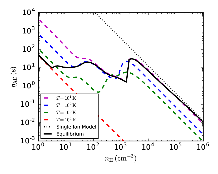
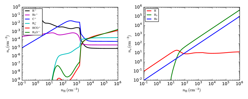
Figure 1 shows the chemical abundances as a function of $n_{\rm H}$ for equilibrium gas temperatures. The plot can roughly be divided into three regimes: the low density gas dominated by protons and neutral atomic hydrogen, the intermediate range where the neutral component is now molecular but the dominant ion is $\rm C^{+}$, and the final region where the ion density is dominated by $\rm HCO^{+}$, $\rm H_{3}O^{+}$ and $\rm H_{3}^{+}$.

Many works adopt a simplified chemical model wherein cosmic ray ionization resulting in a representative ion, often $\rm HCO^{+}$, is balanced with dissociative recombination (Elmegreen, 1979). Adopting the nomenclature of Chen & Ostriker (2012), the resistivity from such a model is given by $\eta_{\rm AD}=B^{2}/c^{2}\alpha\rho_{\rm i}\rho_{\rm n}$ where $\alpha=3.7\times 10^{13}\,{\rm cm^{3}\,s^{-1}\,g^{-1}}$ and the the ion number density is given by $n_{i}=10^{-6}\chi_{i}\left(\rho_{\rm n}/\mu_{\rm n}\right)^{1/2}$. The parameter $\chi_{\rm i}=10^{6}\sqrt{\zeta_{\rm CR}/\alpha_{\rm gas}}$ relates the rates of creation and destruction of the ion species. The value of $\chi_{\rm i}=3$ used by Chen & Ostriker (2012) is adopted for the purpose of comparison.

Figure 2 shows the computed resistivity for a number of fixed temperatures in addition to the resistivity along the equilibrium temperature curve. At high densities where the gas is approximately isothermal, there is good agreement with the single ion model. The models begin to diverge when the primary ions become atomic, with the models further diverging as the gas temperature increases at lower densities.

Table 1: Momentum Exchange Coefficients

Interaction	$\left<\sigma w\right>_{\rm in}$  $\left(\times 10^{-9}\,\,{\rm cm^{3}\,s^{-1}}\right)$	Source	Comment
Collisions with $\rm e^{-}$
$\rm e^{-}$-$\rm H$	$\sqrt{T}\left(2.841+0.093\theta+0.245\theta^{2}-0.089\theta^{3}\right)$	Pinto & Galli (2008)
$\rm e^{-}$-$\rm He$	$0.428\sqrt{T}$	Pinto & Galli (2008)
$\rm e^{-}$-$\rm H_{2}$	$\sqrt{T}\left(0.535+0.203\theta-0.163\theta^{2}+0.050\theta^{3}\right)$	Pinto & Galli (2008)
Collisions with ${\rm H^{+}}$
$\rm H^{+}$-$\rm H$	$0.649T^{0.375}$	Pinto & Galli (2008)
$\rm H^{+}$-$\rm He$	$1.424+7.438\times 10^{-6}T-6.734\times 10^{-9}T^{2}$	Pinto & Galli (2008)
$\rm H^{+}$-$\rm H_{2}$	$1.003+0.050\theta+0.136\theta^{2}-0.014\theta^{3}$	Pinto & Galli (2008)
Collisions with $\rm He^{+}$
$\rm He^{+}$-$\rm H$	$4.71\times 10^{-1}$	Schunk & Nagy (2004)
$\rm He^{+}$-$\rm He$	$2.0\times 8.73\times 10^{-2}(1-0.093\log T)^{2}$	Schunk & Nagy (2004)
Collisions with ${\rm H_{3}^{+}}$
$\rm H_{3}^{+}$-$\rm H_{2}$	$2.693-1.238\theta+0.663\theta^{2}-0.089\theta^{3}$	Pinto & Galli (2008)
Collisions with molecular ions ${\rm M^{+}}$ other than $\rm H_{3}^{+}$
$\rm M^{+}$-$\rm H_{2}$	$\sqrt{T}\left(1.476-1.409\theta+0.555\theta^{2}-0.0775\theta^{3}\right)$	Pinto & Galli (2008)	Adopted rate for $\rm HCO^{+}$
Collisions with atomic ions ${\rm A^{+}}$ other than $\rm H^{+}$, $\rm He^{+}$
$\rm A^{+}$-$\rm H$	$1.983+0.425\theta-0.431\theta^{2}+0.114\theta^{3}$	Pinto & Galli (2008)	Adopted rate for $\rm C^{+}$

Note. — The momentum exchange coefficients are functions of both $T$ and $\theta=\log\left(T/K\right)$.

2.5 Parameter Study

Table 2: Summary of Simulations

Model	Name	$v_{\rm rel}$	B	AD
		$\rm(km\,s^{-1})$	$(\mu G)$
Fiducial B-Field Strength
1	Ideal Colliding	$10$	$10$	No
2	Ideal Non-colliding	$0$	$10$	No
3	AD Colliding	$10$	$10$	Yes
4	AD Non-colliding	$0$	$10$	Yes
Strong B-Field
5	Ideal Colliding	$10$	$30$	No
6	Ideal Non-colliding	$0$	$30$	No
7	AD Colliding	$10$	$30$	Yes
8	AD Non-colliding	$0$	$30$	Yes

A parameter study of eight simulations is performed, varying the magnetic field strength, relative velocity of the clouds (i.e., colliding and non-colliding cases), and whether or not ambipolar diffusion is included. The run parameters are listed in Table 2: the ideal MHD simulations represent a subset of the parameters investigated in Paper II. Each simulation is run for $4\,{\rm Myrs}$, as in Paper II.

3 Results

Analysis of the runs is performed with the goal of specifically comparing the ideal and AD simulation results. Many of the analyses performed in Paper II resulted in limited differences between ideal and AD runs and are thus not discussed here.

The visualizations are made in a rotated coordinate system $\left(x^{\prime},y^{\prime},z^{\prime}\right)$ rotated by $\left(\theta,\phi\right)=\left(15^{\circ},15^{\circ}\right)$ relative to the coordinates $\left(x,y,z\right)$ used in the simulation. This limits the contribution to the projected quantities of the planar density enhancement associated with the colliding ambient medium around the clouds (note, the ambient gas around each GMC, of ten times smaller density, is also assumed to be moving with the same velocity as the GMC). While this enhancement does not contribute significantly to the dynamics, it can be visible in plots of projected quantities due to the long path lengths involved.

To better quantify differences between ideal and AD MHD runs, we focus on density-weighted quantities,

$$\langle X\rangle_{\rho}=\frac{\int X\rho dV}{\int\rho dV},$$ (19)

and their associated variance

$$\sigma^{2}_{X}=\langle X^{2}\rangle_{\rho}-\langle X\rangle_{\rho}^{2}.$$ (20)

Unless otherwise noted, the integrations take place over the central $64^{3}\,{\rm pc^{3}}$.

3.1 Cloud Evolution and the Formation of Dense Cores

3.1.1 Density Distribution Functions

Figure 3 shows the evolution of the mass surface density for each of the AD MHD runs, colliding and non-colliding, over a period of 4 Myr. On these larger scales, cloud evolution progresses in the same basic manner as in Paper II. In the non-colliding simulations overdense regions are created by the converging flows and shocks resulting from the initial internal turbulence that is injected into the GMCs, as well as a modest degree of collapse caused by the GMCs being gravitationally unstable. In the colliding simulations, which Figure 3 shows viewed in a direction perpendicular to the collision axis, a more substantial amount of dense gas is created in the regions of the GMCs compressed by the collision.

Figure 3: Evolution of mass surface density from 1 to 4 Myr (panels left to right) for each AD run. First row: $B=10\>{\rm\mu G}$, colliding; 2nd row: $B=10\>{\rm\mu G}$, non-colliding; 3rd row: $B=30\>{\rm\mu G}$, colliding; bottom row: $B=30\>{\rm\mu G}$, non-colliding. These figures show the overall evolution of cloud structures as a result of internal turbulence and, in the first and third rows, of the 10$\>{\rm km\>s}^{-1}$ GMC-GMC collision. Density differences resulting from AD compared to the ideal MHD case occurring on small scales are presented in the next figures.

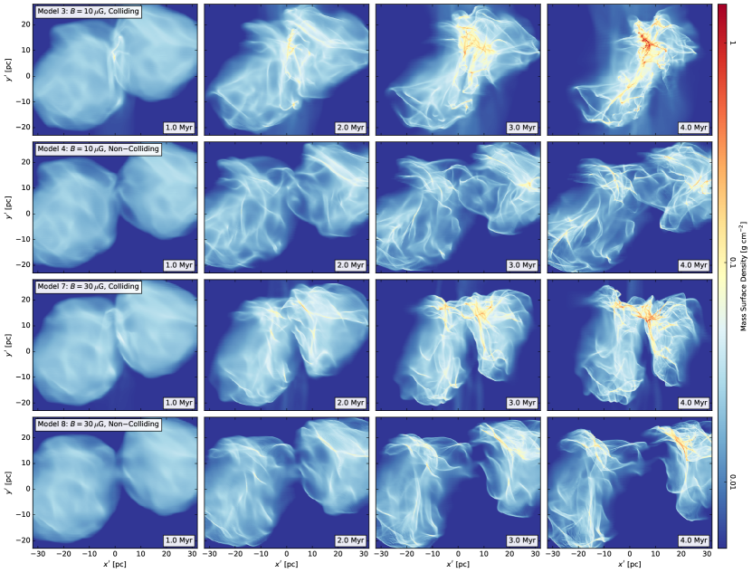
For the $10\,{\rm\mu G}$ cases, there are limited morphological differences between the ideal and AD MHD runs. However, the colliding $30\,{\rm\mu G}$ ideal and AD MHD runs do exhibit more significant qualitative differences. In particular, a larger number of dense cores and filaments are seen to form in the AD simulation. This is illustrated in Figure 6, which zooms in to the main $\sim$25 pc by $\sim$30 pc concentration of dense gas that is created by the GMC-GMC collision. The AD case has $22$ cores with densities $n_{\rm H}\geq 10^{5}\,{\rm cm^{-3}}$, while the ideal case only has $15$ cores at $t=4.0\,\,{\rm Myrs}$. The total mass found in the cores is $3880\,{M_{\odot}}$ for the AD case compared to $1520\,{M_{\odot}}$ for the ideal case. The larger degree of morphological difference in the $30\,{\rm\mu G}$ ideal and AD runs is expected both due to the increased magnetic support and the scaling of resistivity with magnetic field strength, $\eta_{\rm AD}\propto B^{2}$.

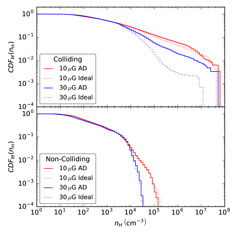
The effects of ambipolar diffusion can also be seen in the cumulative distribution function (CDF) for the gas density. In general, magnetic fields act to inhibit collapse, preventing the gas from reaching higher densities. Thus including ambipolar diffusion should reduce magnetic support and allow higher densities to be achieved. Figure 4 shows the CDFs for the non-colliding and colliding runs at $t=4$ Myr.

For the non-colliding clouds (Figure 4, bottom panel), higher densities are created by local turbulence and gravitational instability set-up as part of the initial conditions. The GMCs threaded by 10 $\rm\mu G$ $B$-fields achieve maximum densities of $n_{\rm H}\sim 10^{5}\>{\rm cm^{-3}}$, while those with 30 $\rm\mu G$ $B$-fields only reach $n_{\rm H}\sim 3\times 10^{4}\>{\rm cm^{-3}}$. Including AD leads to only modest changes in the CDFs.

For the colliding GMCs, much higher densities are achieved by the end of the simulation runs at 4 Myr, which we note is similar to the free-fall time of the initial GMCs, i.e., 4.35 Myr. We consider the mass fraction above densities of $n_{\rm H}=10^{6}\>{\rm cm}^{-3}$, which is a typical density achieved in pre-stellar cores in IRDCs (e.g., Tan et al. 2013; Kong et al. 2017a, b). In the simulations with $B=10\>{\rm\mu G}$, in the ideal case this fraction is about 4%, rising to about 6% when AD is implemented. For the $B=30\>{\rm\mu G}$ runs, the effect of AD is more pronounced. The ideal run has a mass fraction of only 0.2% with $n_{\rm H}>10^{6}\>{\rm cm}^{-3}$, while with AD this increases by about a factor of 10 to 2%. These percentages are similar to the star formation efficiencies per free-fall time inferred from observational studies of GMCs (e.g., Zuckerman & Evans, 1974; Krumholz & Tan, 2007; Lee et al., 2016), however a full quantitative comparison would require simulations that explicitly include star formation from the dense gas and localized feedback from the newly formed stars.

We note that the differences in the CDFs between these four runs start to emerge at densities greater than a few $\times 10^{3}\>{\rm cm}^{-3}$. This is likely to be due in part to the local maxima in the ambipolar resistivity at $n_{\rm H}\sim 3000\,{\rm cm^{-3}}$ (see Figure 2).

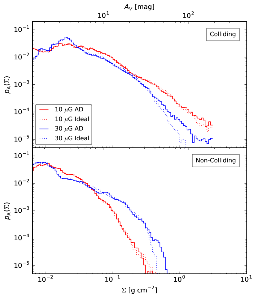
Figure 5 shows the PDF of mass surface density of the central $\left(32\,{\rm pc}\right)^{2}$ regions shown in Figure 3 (and the equivalent regions in the ideal MHD simulations). We observe small differences between the ideal and AD runs for the $10\,{\rm\mu G}$ cases, while in the $30\,{\rm\mu G}$ runs the AD cases consistently have more gas at higher mass surface densities than in their ideal MHD counterparts, and that the deviations become prominent at a few$\times 10^{-1}\,{\rm g\,cm^{-2}}$. This is consistent with the results seen in the PDFs of gas density as well as the qualitative differences seen in Figure 6, which zooms in to part of this region.

In summary, AD can have a significant impact on raising the efficiency of dense, $n_{\rm H}\gtrsim 10^{6}\>{\rm cm}^{-3}$ gas formation in the collision of moderately magnetized, but still supercritical, GMCs. AD would thus also be expected to enhance the star formation activity that arises in such collisions.

Figure 4: Cumulative distribution functions of density for colliding (top panel) and non-colliding (bottom panel) runs at $t=4\,{\rm Myrs}$.

Figure 5: The area weighted $\Sigma$-PDFs for the colliding (top panel) and non-colliding (bottom panel) runs at $t=4.0\,{\rm Myrs}$ for the central $(32\,{\rm pc})^{2}$ regions for each run.

3.1.2 A Sample Core

As a case study, we examine a region of Figure 6 which exhibits core formation in the AD case but no core formation in the ideal case. This region is not necessarily representative, but is presented to highlight differences between the AD and ideal cases.

Figure 7 shows a comparison of an example $4\,{\rm pc}\times 4\,{\rm pc}$ region for both the ideal and AD $B=30\,{\rm\mu G}$ colliding runs. Panel (a) of this figure shows that the AD case exhibits an increased number of high mass surface density ($\Sigma\gtrsim 1.0\,{\rm g\,cm^{-2}}$) structures, including a central core that does not form in the ideal MHD case. This core sits within a dense, branched filament, which is much more pronounced in the AD case. This core also reveals itself as a location of stronger $B$-field strength (panels b and c) and of lower temperature, $T\sim 10\,{\rm K}$ (panel d). Relatively high localized infall velocities (and velocity gradients), including flows along the filament, are also present around the core in the AD simulation (panels e and f).

Figure 6: Comparison of the mass surface densities of the $B=30\,{\rm\mu G}$ ideal (Model 5, left) and $B=30\,{\rm\mu G}$ AD (Model 7, right) colliding cloud cases at $t=4.0\,\,{\rm Myrs}$. The panels show a zoomed-in region centered on the densest gas structures that are created by the collision. Note the presence of a larger number of dense cores in the right panel in the simulation that includes ambipolar diffusion.

Figure 7: A comparison of a $4\,{\rm pc}\times 4\,{\rm pc}$ region for the AD case (left panels in each pair) and the ideal case (right panels in each pair) for the $30\,{\rm\mu G}$ colliding cloud simulations. The region is selected to highlight collapse and fragmentation in the AD MHD run that is not found in the ideal MHD run. (a) Mass surface density. The overplotted streamlines follow the magnetic field lines. (b) Density-weighted line of sight magnetic field ($B_{z}$). (c) Density-weighted plane of sky magnetic field strength. (d) Density-weighted temperature. (e) Density-weighted line of sight velocity. (f) Density-weighted plane-of-sky velocity. Vectors indicate the direction of the flow.

Figure 8: Density slices along each cardinal direction centered on the central core in the AD simulation (Model 7) in Figure 7. Arrows indicate the local velocity. The largest projected velocity in each slice is approximately $10\,{\rm km\,s^{-1}}$.

Figure 9: Density (top panel), velocity (middle panel), and local Alfvén speed (bottom panel) profiles along each axis through the center of the core in Figure 8. The coordinates are normalized so that the density peak is at the origin, and the velocities are in the frame of the density peak. In the middle panel, the dashed line shows the free fall speed $v_{\rm ff}=\sqrt{2GM_{\rm enc}/R}$.

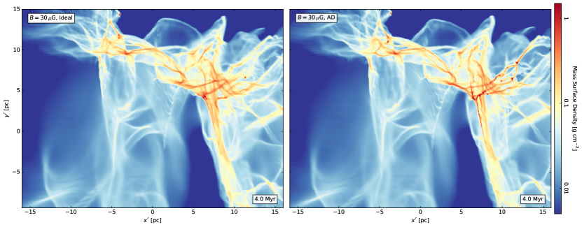
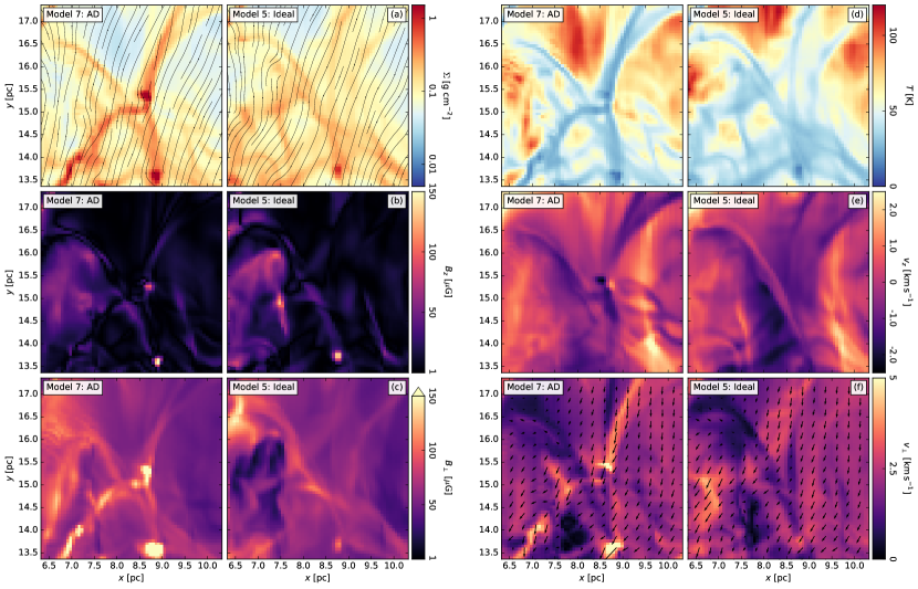
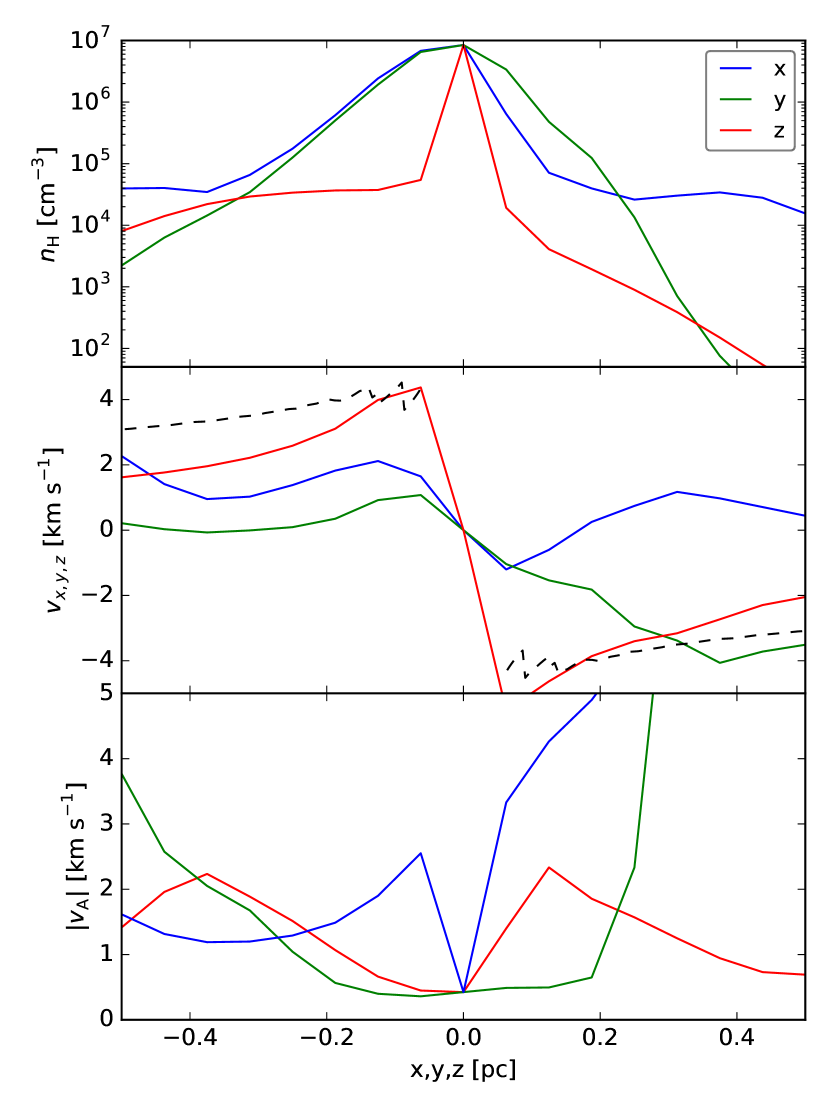
Figure 8 shows density slices through the central core formed in the $30\,{\rm\mu G}$ AD run in the field shown in Figure 7. The core exhibits a flattened disk-like morphology, i.e., being elongated in the $x$-$y$ plane, and appears to be accreting from surrounding filamentary structures. The velocity flow patterns generally show infall to the core, but there are also strong velocity gradients seen in the $x$-$y$ plane indicating a degree of rotational support.

In Figure 9 we plot density and velocity profiles along the coordinate axes centered on the core. The relatively extended density structures in the $x$ and $y$ directions compared to the $z$ direction are apparent. Infall velocities are supersonic and trans-Alfvénic. However, relative to the free-fall velocity $v_{\rm ff}=\sqrt{2GM_{\rm enc}/R}$ for a sphere of radius $R$ and associated enclosed mass $M_{\rm enc}$, the velocities along the $x$ and $y$ axes are a factor of several below $v_{\rm ff}$, while along the $z$ axis, the velocities can be comparable to $v_{\rm ff}$.

3.2 Magnetic Fields

3.2.1 The $B$ vs $n_{\rm H}$ Relation

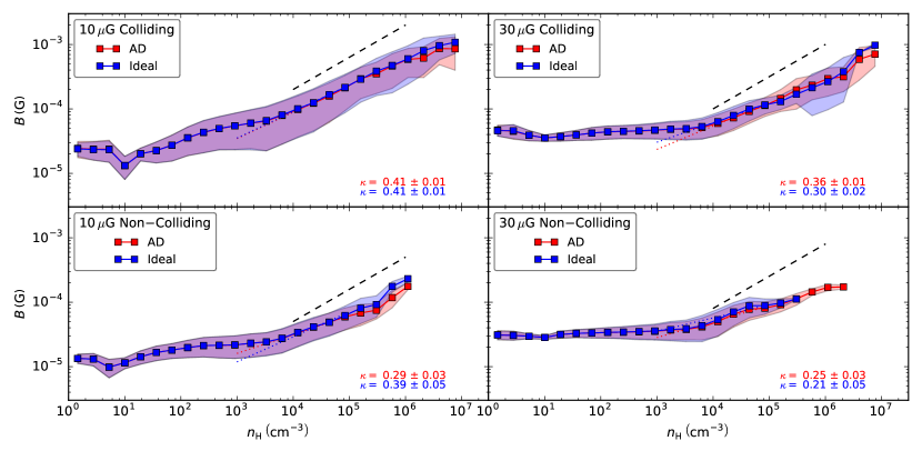
We examine how the magnetic field strength varies with gas density. Figure 10 shows the density-weighted average magnetic field strength as a function of $n_{\rm H}$ for the simulation outputs at 4 Myr. It also shows the dispersion, $\pm\sigma_{B}$, of the field strength about this average. The ideal and AD runs show similar behavior over most of the density range, with deviations confined to the highest densities, in part because runs with AD are able to achieve higher densities, i.e., in the non-colliding $B=30\>{\rm\mu G}$ case. At low densities, i.e., material external to the initial GMCs, the field strength is observed to remain approximately constant. Then in the weaker, $10\>{\rm\mu G}$ initial field case, the field strength is seen to start increasing at densities of $n_{\rm H}\sim 100\>{\rm cm}^{-3}$ in the colliding GMCs, but at higher densities in the non-colliding simulation. In the $30\>{\rm\mu G}$ cases, the gas density above which the $B$-field strength is seen to start rising is higher still, i.e., at several $\times 10^{3}\>{\rm cm}^{-3}$.

The black dashed lines in Figure 10 show a scaling $B\propto n_{\rm H}^{\kappa}$ with $\kappa=0.5$, which is the prediction of some models of clouds with trans-Alfvénic turbulence (e.g., Mocz et al. 2017). Note that clouds with super-Alfvénic turbulence are expected to have a steeper relation with $\kappa\simeq 2/3$ (Li et al. 2015; Mocz et al. 2017). There is expected to be a small decrease in $\kappa$ due to ambipolar diffusion. Fiedler & Mouschovias (1993) found AD causes $\kappa$ to drop from 0.50 to $0.44$-$0.50$ within the context of axisymmetric, isothermal collapse. In our simulations, the equilibrium temperature decreases from $20\,{\rm K}$ at $n_{\rm H}=10^{3}\,{\rm cm^{-3}}$ to $7\,{\rm K}$ at $n_{\rm H}=10^{6}\,{\rm cm^{-3}}$. For polytropes of the form $P\propto\rho^{\gamma}$, the expected magnetic field scaling becomes $B\propto\rho^{\gamma/2}$ which would imply a smaller value of $\kappa$ for gas that is cooling during its collapse. This effect may explain, at least in part, why for all our simulation cases, the actual magnetic field strength scales with an exponent less than $1/2$, i.e., we find $\kappa\simeq 0.2$ to 0.4 (measured over the range $10^{3}\>{\rm cm}^{-3}<n_{\rm H}<10^{5}\>{\rm cm}^{-3}$).

Figure 10: The distribution of magnetic field strengths as a function of gas density for the four simulation set-ups, each with and without AD. Solid squares show the density-weighted mean magnetic field for ideal (blue) and AD (red) MHD runs. The shaded regions show the $\pm 1\sigma_{\rm B}$ dispersion of magnetic field strengths about this average. The dashed black line shows the scaling $B\propto n_{\rm H}^{1/2}$. The dotted lines are fits to the respective density-weighted lines between $n_{\rm H}=10^{3}\,{\rm cm^{-3}}$ to $10^{5}\,{\rm cm^{-3}}$ with the associated power-law scaling listed in the lower right corner.

3.2.2 The Mass-to-Flux Ratio of Cells

Paper III developed a star formation subgrid model in which only cells achieving a particular mass-to-flux ratio $\mu_{\rm cell}$ are allowed to form star particles. This model defines the in-cell mass-to-flux ratio $\mu_{\rm cell}$ as

$$\mu_{\rm cell}=\frac{\Delta x\rho\sqrt{G}}{c_{1}B},$$ (21)

where $c_{1}$ is the geometry-dependent factor establishing the critical value, with the adopted value here being $c_{1}=1/\sqrt{63}$ as in equation 1. There are a number of caveats concerning the quantity $\mu_{\rm cell}$. As defined, $\mu_{\rm cell}$ is inherently a local, numerical construct and is not related to the stability of a self-gravitating object.

The explicit dependence on $\Delta x$ means its value will depend on the resolution at which it is evaluated. It does, however, have potential value as input for a subgrid star formation model, which aims to have sensitivity to the degree of local magnetic support in the gas.

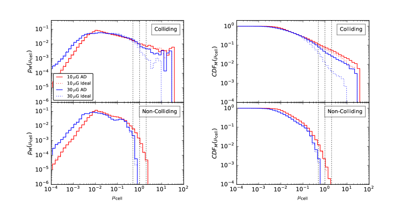
Given that the simulations of Paper III were done in the limit of ideal MHD, how $\mu_{\rm cell}$ changes in the limit of explicit non-ideal MHD, i.e., with AD, is of interest. Figure 11 shows the density-weighted distributions for $\mu_{\rm cell}$ for the colliding and non-colliding cases. The non-colliding cases exhibit relatively minor differences in the distribution of $\mu_{\rm cell}$ for the ideal and AD cases, as would be expected given the small changes in volume density distributions. The $30\,{\rm\mu G}$ colliding case exhibits the greatest differences between the ideal and AD runs with approximately four times as much mass in supercritical cells in the AD MHD case compared to the ideal MHD case. This would lead to correspondingly higher levels of star formation activity in simulations using such a subgrid model. Simulations with AD and star formation will be presented in a future paper in this series.

Figure 11: The mass-weighted PDF (left column) and CDF (right column) for the in-cell mass-to-flux ratios for all colliding (top row) and non-colliding (bottom row) runs. The three vertical dotted lines represent values of $\mu_{\rm cell}=0.5$, $1.0$, and $2.0$, the threshold values for star formation used in Paper III.

3.2.3 Relative Orientations: B vs N

Figure 12: The histogram shape parameters $\xi$ vs column density $N_{\rm H}$ for each of the colliding runs. The blue, green, and red lines represent the lines of sight along the $x^{\prime}$, $y^{\prime}$, and $z^{\prime}$ axes, respectively. The fitting parameters for each line of sight is labelled in its respective color.

As in Paper II, the magnetic field orientations are investigated via the Histogram of Relative Orientations (HRO, Soler et al. 2013). The HRO quantifies the relative orientation between the filamentary structures seen in column density $N_{\rm H}$ and the plane-of-sky polarization,

$$\phi=\arctan\left(\frac{\boldsymbol{\nabla}N_{\rm H}\cdot\boldsymbol{p}}{|\boldsymbol{\nabla}N_{\rm H}\times\boldsymbol{p}|}\right).$$ (22)

The polarization $\boldsymbol{p}$ is a pseudo-vector defined by

$$\boldsymbol{p}=\left(p\sin\chi\right)\boldsymbol{x}+\left(p\cos\chi\right)\boldsymbol{y},$$ (23)

where $p$ is the polarization fraction and $\chi$ is the polarization angle. A discussion of the calculation of $\chi$ can be found in Paper II. The HRO is then created from the distribution of angles $\phi$.

The convexity of the HRO is defined by the shape parameter,

$$\xi=\frac{A_{\rm c}-A_{\rm e}}{A_{\rm c}+A_{\rm e}},$$ (24)

where $A_{\rm c}$ is the area under the central region ($-22.5^{\circ}<\phi<22.5^{\circ}$) and $A_{\rm e}$ is the area under the extrema ($-90^{\circ}<\phi<-22.5^{\circ}$ and $22.5^{\circ}<\phi<90^{\circ}$). Within this formalism, $\xi>0$ indicates a concave histogram with $\boldsymbol{p}$ perpendicular to the iso-$N_{\rm H}$ contours while $\xi<0$ indicates a convex histogram with $\boldsymbol{p}$ parallel to the iso-$N_{\rm H}$ contours.

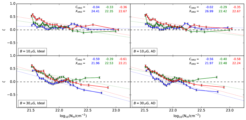
Figure 12 shows $\xi$ as a function of $N_{\rm H}$ for all the colliding runs in the parameter study, along with fits taking the form

$$\xi\left(N_{\rm H}\right)=C_{\rm HRO}\left[\log\left(N_{\rm H}/{\rm cm^{2}}\right)-X_{\rm HRO}\right].$$ (25)

The same trends found in Paper II for ideal magnetohydrodynamics are found in the runs in this paper, although the parameters for the fits are slightly different, which can be attributed to the changes in numerical methods outlined in previous sections. Between ideal and AD runs, there appears to be little difference, except for small increases in $\xi$ at the highest column densities.

3.3 Temperature Structure and Resistive Heating

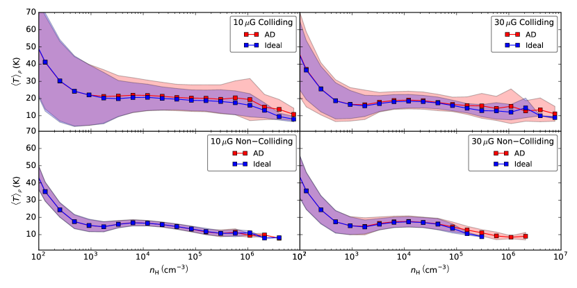
Localized variations of temperature in the ideal and AD runs were already apparent in Figure 7d, but were driven mostly by the variation in local density structures that arose between the two simulations. To determine the effect of ambipolar diffusion heating, we examine the density-weighted temperature $\langle T\rangle_{\rho}$ for both the ideal and AD runs. Figure 13 shows $\langle T\rangle_{\rho}$ for each run as well as the $1\sigma$ dispersion about these averages. From comparison with the equilibrium temperature versus density relation (Paper I), we see that the majority of the mass stays close to thermal equilibrium. However, runs with ambipolar diffusion tend to exhibit a consistent increase in temperature for $n_{\rm H}\gtrsim 10^{3}\,{\rm cm^{-3}}$, with more significant temperature increases seen in the colliding runs and/or the more strongly magnetized cases.

Resistive heating has a limited effect on gas at densities below $10^{3}\,{\rm cm^{-3}}$. Compared to their non-colliding counterparts, colliding clouds exhibit more significant resistive heating, as would be expected given the magnetic field gradients generated in the collision and collapse. Additionally, the stronger field cases exhibit more significant heating, with temperature increases approaching $10\%$, as would be expected given the increased resistivity ($\eta_{\rm AD}\propto B^{2}$).

As with the differences in the density distribution, the increased role of resistive heating at $\sim 10^{3}\,{\rm cm^{-3}}$ is due to the peak in resistivity caused by the transition from being dominated by atomic ions to being dominated by molecular ions.

Figure 13: The density-weighted temperature for ideal (blue) and AD (red) MHD runs (panels, as labelled). The shaded regions show the $\pm 1\sigma_{\rm T}$ dispersion around these average temperatures.

4 Discussion and Conclusions

In this paper we have developed and implemented ambipolar diffusion in the Enzo code. We have then investigated the role of ambipolar diffusion in collisions between GMCs, using resistivities calculated from the chemical model of Paper I.

The strongest effects of ambipolar diffusion are seen in the simulations of colliding GMCs that start with mean $B$-fields of 30 $\rm\mu G$ (i.e., the strong field case), although note that these GMCs are still magnetically supercritical. The formation of dense, $\gtrsim 10^{6}\>{\rm cm}^{-3}$ gas is greatly promoted, by factors of $\sim 10$, in the simulation that includes ambipolar diffusion. One may expect that such differences would also extend to star formation rates in these GMCs, to be investigated in a future paper in this series. In the simulations with initial $B$-field strengths of 10 $\rm\mu G$, the GMCs are initially magentically supercritical to a greater degree and ambipolar diffusion plays a smaller role.

Resistive heating that arises in the AD simulations also has only a minor influence on the mass-averaged temperatures, although excursions to higher temperatures are seen, e.g., in the $1\sigma$ dispersion, which may have important implications for astrochemical processes, such as CO freeze-out, normally expected to occur for $T\lesssim 20\>$K.

Since some recent studies of IRDCs have inferred $\sim{\rm mG}$ $B$-field strengths (Pillai et al., 2015, 2016) and thus trans- or sub-Alfvénic turbulence, there may be an important role for non-ideal MHD processes, such as ambipolar diffusion, in regulating star formation activity in such systems. Other non-ideal MHD processes, such as reconnection diffusion (Lazarian & Vishniac, 1999; Eyink et al., 2011), may also need to be considered for a complete understanding of the star formation process in such systems.

Appendix A Tests of the Ambipolar Diffusion Module

A.1 C-Shock Test

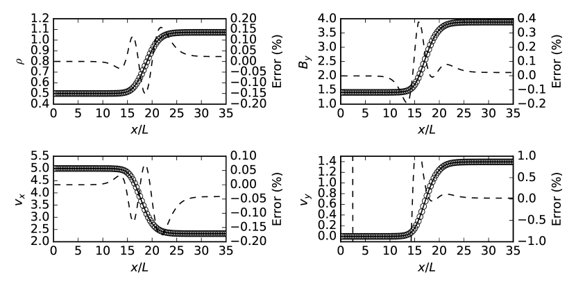
The case of a C-shock can be solved semi-analytically and has been used as a test case for implementations of ambipolar diffusion (Mac Low et al., 1995). Mac Low et al. (1995) provide a semi-analytic solution in the form of a first-order ordinary differential equation,

$$\left(\frac{1}{\bar{\rho}^{2}}-\frac{1}{M_{\rm s}^{2}}\right)L\frac{\partial\bar{\rho}}{\partial x}=\frac{b_{y}}{M_{\rm A}\left(b_{y}^{2}+\cos^{2}\theta\right)}\left(b_{y}-\bar{\rho}\left(\frac{b_{y}-b_{y,0}}{M_{\rm A}^{2}}\cos^{2}\theta+\sin\theta\right)\right),$$ (A1)

where dimensionless density is $\bar{\rho}=\rho/\rho_{0}$, and the dimensionless, perpendicular component of the magnetic field is $b_{y}=B_{y}/B_{0}$. $b_{y,0}=\sin\theta$. The sonic and Alfvén Mach numbers are given by $M_{\rm s}=v_{s}/c_{s}$ and $M_{\rm A}=v_{s}/v_{{\rm A},0}$, respectively. The shock length scale is $L=D/v_{{\rm A},0}=B_{0}/\left(\gamma\rho_{i}\sqrt{4\pi\rho_{0}}\right)$. The system is closed with the auxiliary equation

$$b_{y}^{2}=b_{y,0}^{2}+2M_{\rm A}^{2}\left(\bar{\rho}-1\right)\left(\frac{1}{\bar{\rho}}-\frac{1}{M_{\rm s}^{2}}\right).$$ (A2)

Equation A1 can be integrated to get a final steady-state solution.

To generate the C-shock in the simulation, a one-dimensional shock tube is initialized with a discontinuity at the midpoint and the upwind and downwind fluid variables given in Table 3. The system is then allowed to evolve and the results are fit to the semi-analytic solution derived from equations A1 and A2. The results are shown in Figure 14 and are in excellent agreement.

Table 3: C-Shock Initial Conditions

	Upwind Value	Downwind Value
$\rho\,({\rm g\,cm^{-3}})$	$0.5$	$1.0727$
$B_{x}\,({\rm G})$	$5.01325$	$5.01325$
$B_{y}\,({\rm G})$	$5.01325$	$13.7574$
$v_{x}\,({\rm cm\,s^{-1}})$	$5.0$	$2.3305$
$v_{y}\,({\rm cm\,s^{-1}})$	$0$	$1.3953$

Figure 14: The density, perpendicular magnetic field, and velocity components from the C-shock test. The results of the test are shown as open circles while the solution to Eqn. A1 is shown a solid line. The dashed line indicates the relative error.

A.2 Protostellar Collapse: Isothermal Case

To set up a protostellar collapse, a cylinder of density $\rho=1.167\times 10^{-21}\,{\rm g\,cm^{-3}}$ with radius of $0.75\,{\rm pc}$ and height $1.5\,{\rm pc}$ is placed within a cubic computational domain of side $2\,{\rm pc}$. A uniform $20\,{\rm\mu G}$ magnetic field is initialized along the cylinder’s axis. This results in an initial dimensionless mass-to-flux ratio $\mu_{0}=0.55$.

The top grid resolution is $128^{3}$ with grid refinement done to ensure that the local Jeans length is resolved with at least 8 zones per Jeans length. A maximum of 6 levels of refinement are used resulting in a top grid size of $0.0325\,{\rm pc}$ and a grid size of $4.88\times 10^{-4}\,{\rm pc}$ on the finest grid. To facilitate comparison with other similar non-turbulent collapse models, the resistivity is taken to be of the form $\eta_{\rm AD}=\min\left(100,29B^{2}/\rho^{3/2}\right)$. The maximum value placed on $\eta_{\rm AD}$ both mimics the role of UV in increasing the ionization and prevents the resistivity from becoming prohibitively large in low density regions.

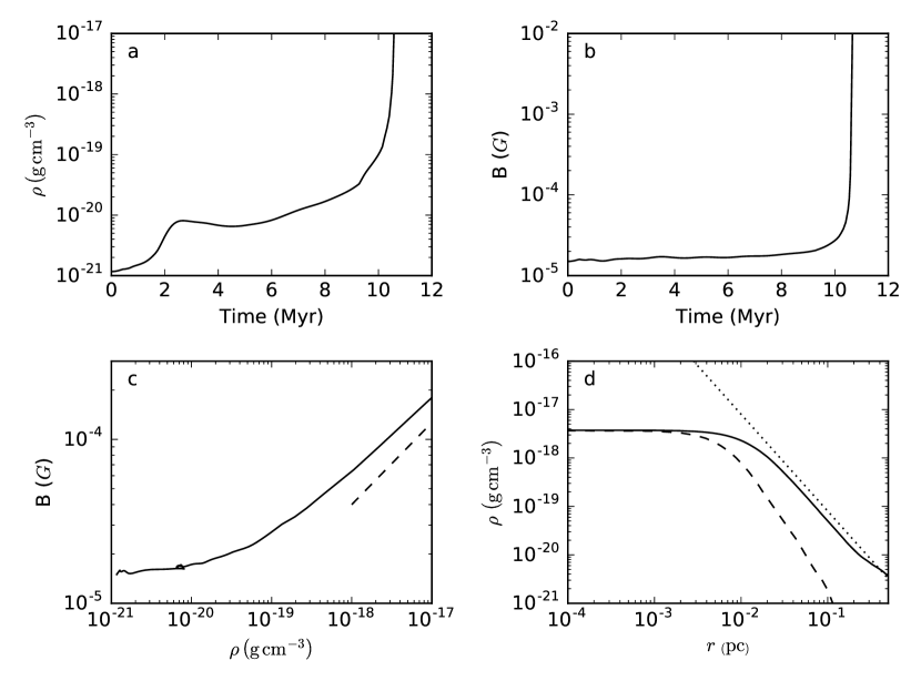
The results are shown in Figure 15. As has been seen in similar axisymmetric models, the gas initially collapses along the magnetic field, resulting in a bounce just after $t=2\,{\rm Myrs}$, as can be seen in Figure 15a. Via ambipolar diffusion, gravity draws gas through the field, increasing the central density while leaving the magnetic field strength roughly unchanged (see Figure 15b). Once sufficient gas has been accumulated (around $11\,{\rm Myrs}$), runaway collapse begins with central density and magnetic field strength increasing dramatically.

Figure 15c shows the $B-\rho$ relation for the central density and magnetic field. Once dynamic collapse begins, the magnetic field scales roughly $\rho^{1/2}$, with the scaling being slightly shallower than the expected $B\propto\rho^{1/2}$ scaling due to the continued action of ambipolar diffusion during the collapse. Figure 15d shows the profiles through the center-of-mass of the cloud at $t=11\,{\rm Myrs}$. Along directions perpendicular to the initial magnetic field, the density decreases as $\rho\propto r^{-2}$, as expected.

Figure 15: The results the collapse test. (a) The time evolution of the peak gas density. (b) The time evolution of the peak magnetic field strength. (c) The magnetic field strength as a function of peak gas density (solid line). The dashed line shows a scaling of $B\propto\rho^{1/2}$. (d) density profiles through the center of the profile perpendicular to the initial magnetic field direction (solid line) and parallel to the initial field direction (dashed line). The dotted line shows a $\rho\propto r^{-2}$ scaling.

References

- Chen & Ostriker (2012) Chen, C.-Y., & Ostriker, E. C. 2012, ApJ, 744, 124
- Crutcher (1999) Crutcher, R. M. 1999, ApJ, 520, 706
- Crutcher et al. (2009) Crutcher, R. M., Hakobian, N., & Troland, T. H. 2009, ApJ, 692, 844
- Crutcher et al. (2010) Crutcher, R. M., Wandelt, B., Heiles, C., Falgarone, E., & Troland, T. H. 2010, ApJ, 725, 466
- Dedner et al. (2002) Dedner, A., Kemm, F., Kröner, D., et al. 2002, Journal of Computational Physics, 175, 645
- Elmegreen (1979) Elmegreen, B. G. 1979, ApJ, 232, 729
- Eyink et al. (2011) Eyink, G. L., Lazarian, A., & Vishniac, E. T. 2011, ApJ, 743, 51
- Falgarone et al. (2008) Falgarone, E., Troland, T. H., Crutcher, R. M., & Paubert, G. 2008, A&A, 487, 247
- Federrath et al. (2011) Federrath, C., Sur, S., Schleicher, D. R. G., Banerjee, R., & Klessen, R. S. 2011, ApJ, 731, 62
- Ferland et al. (2013) Ferland, G. J., Porter, R. L., van Hoof, P. A. M., et al. 2013, Rev. Mexicana Astron. Astrofis., 49, 137
- Fiedler & Mouschovias (1993) Fiedler, R. A., & Mouschovias, T. C. 1993, ApJ, 415, 680
- Heiles & Troland (2005) Heiles, C., & Troland, T. H. 2005, ApJ, 624, 773
- Hezareh et al. (2014) Hezareh, T., Csengeri, T., Houde, M., Herpin, F., & Bontemps, S. 2014, MNRAS, 438, 663
- Hezareh et al. (2010) Hezareh, T., Houde, M., McCoey, C., & Li, H.-b. 2010, ApJ, 720, 603
- Kong et al. (2017a) Kong, S., Tan, J. C., Caselli, P., et al. 2017a, ApJ, 834, 193
- Kong et al. (2017b) —. 2017b, ArXiv e-prints, arXiv:1701.05953
- Krumholz & Tan (2007) Krumholz, M. R., & Tan, J. C. 2007, ApJ, 654, 304
- Lazarian & Vishniac (1999) Lazarian, A., & Vishniac, E. T. 1999, ApJ, 517, 700
- Lee et al. (2016) Lee, E. J., Miville-Deschênes, M.-A., & Murray, N. W. 2016, ApJ, 833, 229
- Li et al. (2014) Li, H.-B., Goodman, A., Sridharan, T. K., et al. 2014, Protostars and Planets VI, 101
- Li & Houde (2008) Li, H.-b., & Houde, M. 2008, ApJ, 677, 1151
- Li et al. (2010) Li, H.-b., Houde, M., Lai, S.-p., & Sridharan, T. K. 2010, ApJ, 718, 905
- Li et al. (2015) Li, P. S., McKee, C. F., & Klein, R. I. 2015, MNRAS, 452, 2500
- Li et al. (2012) Li, P. S., Myers, A., & McKee, C. F. 2012, ApJ, 760, 33
- Mac Low et al. (1995) Mac Low, M.-M., Norman, M. L., Konigl, A., & Wardle, M. 1995, ApJ, 442, 726
- McKee (1989) McKee, C. F. 1989, ApJ, 345, 782
- Mestel (1966) Mestel, L. 1966, MNRAS, 133, 265
- Mestel & Spitzer (1956) Mestel, L., & Spitzer, Jr., L. 1956, MNRAS, 116, 503
- Mocz et al. (2017) Mocz, P., Burkhart, B., Hernquist, L., McKee, C. F., & Springel, V. 2017, ApJ, 838, 40
- Mouschovias et al. (2011) Mouschovias, T. C., Ciolek, G. E., & Morton, S. A. 2011, MNRAS, 415, 1751
- Mouschovias & Spitzer (1976) Mouschovias, T. C., & Spitzer, Jr., L. 1976, ApJ, 210, 326
- Mouschovias & Tassis (2009) Mouschovias, T. C., & Tassis, K. 2009, MNRAS, 400, L15
- Mouschovias & Tassis (2010) —. 2010, MNRAS, 409, 801
- Padoan et al. (2000) Padoan, P., Zweibel, E., & Nordlund, Å. 2000, ApJ, 540, 332
- Padoan et al. (2012) —. 2012, ApJ, 755, 182
- Parks (1991) Parks, G. K. 1991, Physics of space plasmas - an introduction (Redwood City, CA: Addison-Wesley Publishing Co.)
- Pillai et al. (2015) Pillai, T., Kauffmann, J., Tan, J. C., et al. 2015, ApJ, 799, 74
- Pillai et al. (2016) Pillai, T., Kauffmann, J., Wiesemeyer, H., & Menten, K. M. 2016, A&A, 591, A19
- Pinto & Galli (2008) Pinto, C., & Galli, D. 2008, A&A, 484, 17
- Schunk & Nagy (2004) Schunk, R. W., & Nagy, A. F. 2004, Ionospheres (Cambridge, UK: Cambridge University Press), 570
- Scoville et al. (1986) Scoville, N. Z., Sanders, D. B., & Clemens, D. P. 1986, ApJ, 310, L77
- Smith et al. (2017) Smith, B. D., Bryan, G. L., Glover, S. C. O., et al. 2017, MNRAS, 466, 2217
- Soler et al. (2013) Soler, R., Carbonell, M., & Ballester, J. L. 2013, ApJS, 209, 16
- Tan (2000) Tan, J. C. 2000, ApJ, 536, 173
- Tan et al. (2014) Tan, J. C., Beltrán, M. T., Caselli, P., et al. 2014, Protostars and Planets VI, 149
- Tan et al. (2013) Tan, J. C., Kong, S., Butler, M. J., Caselli, P., & Fontani, F. 2013, ApJ, 779, 96
- Tassis et al. (2012a) Tassis, K., Willacy, K., Yorke, H. W., & Turner, N. J. 2012a, ApJ, 753, 29
- Tassis et al. (2012b) —. 2012b, ApJ, 754, 6
- Tritsis et al. (2015) Tritsis, A., Panopoulou, G. V., Mouschovias, T. C., Tassis, K., & Pavlidou, V. 2015, MNRAS, 451, 4384
- Turk et al. (2011) Turk, M. J., Smith, B. D., Oishi, J. S., et al. 2011, ApJS, 192, 9
- Wang & Abel (2009) Wang, P., & Abel, T. 2009, ApJ, 696, 96
- Wu et al. (2017a) Wu, B., Tan, J. C., Christie, D., et al. 2017a, ApJ, 841, 88
- Wu et al. (2017b) Wu, B., Tan, J. C., Nakamura, F., et al. 2017b, ApJ, 835, 137
- Wu et al. (2015) Wu, B., Van Loo, S., Tan, J. C., & Bruderer, S. 2015, ApJ, 811, 56
- Zhao et al. (2016) Zhao, B., Caselli, P., Li, Z.-Y., et al. 2016, MNRAS, 460, 2050
- Zuckerman & Evans (1974) Zuckerman, B., & Evans, II, N. J. 1974, ApJ, 192, L149