A sharp oracle inequality for Graph-Slope
Abstract
Following recent success on the analysis of the Slope estimator, we provide a sharp oracle inequality in term of prediction error for Graph-Slope, a generalization of Slope to signals observed over a graph. In addition to improving upon best results obtained so far for the Total Variation denoiser (also referred to as Graph-Lasso or Generalized Lasso), we propose an efficient algorithm to compute Graph-Slope. The proposed algorithm is obtained by applying the forward-backward method to the dual formulation of the Graph-Slope optimization problem. We also provide experiments showing the practical applicability of the method.
keywords:
[class=MSC]keywords:
and
and
t1J. Salmon and S. Vaiter were supported by the CNRS PE1 “ABS” grant.
1 Introduction
Many inference problems of interest involve signals defined on discrete graphs. This includes for instance two-dimensional imaging but also more advanced hyper-spectral imaging scenarios where the signal lives on a regular grid. Two types of structure arise naturally in such examples: The first type of structures comes from regularity or smoothness of the signal, which led to the development of wavelet methods. The second type of structure involves signals with few sharp discontinuities. For instance in one dimension, piecewise constant signals appear when transition states are present, the graph being a 1D path. In imaging, where the underlying graph is a regular 2D grid, occlusions create piece-wise smooth signals rather than smooth ones.
This paper studies regularizers for signals with sharp discontinuities. A popular choice in imaging is the Total Variation (TV) regularization [24]. For 1D signals, TV regularization has also long been used in statistics [18]. If an additional regularization is added, this is sometimes referred to as the fused Lasso [30, 32, 13].
A natural extension of such methods to arbitrary graphs relies on analysis penalties [15] which involve the incidence matrix of the underlying graph, see for instance [25] or the Edge Lasso of [26]. Such penalties have the form
| (1.1) |
where is a tuning parameter and is the (edge-vertex) incidence matrix of the graph defined below, and represents the signal to be recovered. This approach is notably different from contributions in machine learning where penalties, i.e., Laplacian regularization, have been considered for spectral clustering [27, 20] (see also [33] for a review). Theoretical results in favor of the norm instead of the squared norm are studied in [25].
Penalties based on regularization with the graph incidence matrix have recently been analyzed [16], including an analysis of their approximation algorithm. They are of interest as they do not suffer from the (shrinkage) bias created by the convex norm. However, such methods present the difficulty that in the general case they lead to non-convex problems. Note that the 1D path is an exception since the associated optimization problem can be solve using dynamic programming [1]. Concerning the bias reduction though, simpler remedies could be used, including least-squares refitting on the model space associated, applying for instance the CLEAR method [14].
Following the introduction of the Slope regularization in the context of high dimensional regression [10], we propose Graph-Slope, its generalization to contexts where the signal is supported on a graph. In linear regression, Slope [10] is defined as follows. Given tuning parameters with at least one strict inequality, define the ordered norm by
| (1.2) |
where for any , we use the notation111following the notation considered in [7] for the non-increasing rearrangement of its amplitudes . Then, given a design matrix and a response vector , the Slope estimator is defined as a solution of the minimization problem
| (1.3) |
If the parameters are all equal, then Slope is equal to the Lasso with tuning parameter .
Slope presents several advantages compared to Lasso in sparse linear regression. First, Slope provably controls the False Discovery Rate (FDR) for orthogonal design matrices [10] and experiments show that this property is also satisfied for some non-orthogonal design matrices [10]. Second, it appears that Slope has more power than Lasso in the sense that Slope will discover more nonzero coefficients of the unknown target vector [10]. An interpretation of this phenomenon is that Lasso shrinks small coefficients too heavily and may thus miss the smallest nonzero coefficients of the target vector. On the other hand, the Slope penalty induces less shrinkage on small coefficients, leading to more power. Third, while Lasso with the universal parameter is known to achieve the rate of estimation of order (where is the sparsity of the unknown target vector, the number of measurements and the number of covariates), Slope achieves the optimal rate of estimation of order [28, 4].
We propose a theoretical and experimental analysis of Graph-Slope, the counterpart estimator of Slope for signals defined on graphs. Graph-Slope is defined in the next section. Our theoretical contribution for Graph-Slope borrows some technical details recently introduced in [17] to control the Mean Squared Error (MSE) for the Generalized Lasso.
Last but not least, we provide an efficient solver to compute the Graph-Slope estimator. It relies on accelerated proximal gradient descent to solve the dual formulation [3, 12, 22]. To obtain an efficient solver, we leverage the seminal contribution made in [36] showing the link between ordered norm (1.2) and isotonic regression. Hence, we can use fast implementations of the PAVA algorithm (for Pool Adjacent Violators Algorithm, see for instance [6]), available for instance in scikit-learn [23] for this purpose. Numerical experiments illustrate the benefit of Graph-Slope, in particular in terms of True Discovery Rate (TDR) performance.
A high level interpretation of our simulation results is as follows. In the model considered in this paper, a sharp discontinuity of the signal corresponds to an edge of the graph with nonzero coefficient. Since Graph-Lasso uses an -penalty, the penalty level is uniform across all edges of the graph. Edges with small coefficients are too heavily penalized with Graph-Lasso. Using Graph-Slope lets us reduce the penalty level on the edges with small coefficients. This leads to the discovery of more discontinuities of the true signal as compared to Graph-Lasso.
1.1 Model and notation
Let be an undirected and connected graph on vertices, , and edges, . This graph can be represented by its edge-vertex incidence matrix (we drop the reference to when no ambiguity is possible) defined as
| (1.4) |
where . The matrix is the so-called graph Laplacian of . The Laplacian is invariant under a change of orientation of the graph.
For any , we denote by the pseudo norm of : , and for any matrix , we denote by its Moore-Penrose pseudo-inverse. The canonical basis of is denoted .
For any norm on , the associated dual norm reads at
| (1.5) |
As a consequence, for every , one has .
In this work, we consider the following denoising problem for a signal over a graph. Assume that each vertex of the graph carries a signal . For each vertex of the graph, one observes , a noisy perturbation of . In vector form, one observes the vector and aims to estimate , i.e.,
| (1.6) |
where is a noise vector. We will say that an edge of the graph carries the signal . In particular, if two vertices and are neighbours and if they carry the same value of the signal, i.e., , then the corresponding edge carries the constant signal. The focus of the present paper is on signals that have few discontinuities. A signal has few discontinuities if has few nonzero coefficients, i.e., is small, or equivalently if most edges of the graph carry the constant signal. In particular, if , we say that is a vector of -sparsity .
1.2 The Graph-Slope estimator
We consider in this paper the so-called Graph-Slope variational scheme:
| (1.7) |
where
| (1.8) |
with satisfying , and using for any vector the notation222following the notation from [7]. for the non-increasing rearrangement of its amplitudes . According to [10], is a norm over if and only if with at least one strict inequality. This is a consequence of the observation that if then one can rewrite the Slope-norm of as the maximum over all (the set of permutations over ), of the quantity :
| (1.9) |
The Generalized Lasso (also sometimes referred to as TV denoiser) relies on regularization. It was recently investigated in [17, 25], and can be defined as
| (1.10) |
where is the standard norm, and is a tuning parameter.
If then for all , so that the minimization problems (1.10) and (1.7) are the same. On the other hand, if for some , then the optimization problems (1.10) and (1.7) differ. For instance, if , all coefficients of are equally penalized in the Graph-Lasso (1.10), while coefficients of are not uniformly penalized in the Graph-Slope optimization problem (1.7). Indeed, in the Graph-Slope optimization problem (1.7), the largest coefficient of is penalized as in (1.10) but smaller coefficients of receive a smaller penalization. The Graph-Slope optimization problem (1.7) is more flexible than (1.10) as it allows the smaller coefficients of to be less penalized than its larger coefficients. We will see in the next sections that this flexibility brings advantages to both the theoretical properties of as well as its performance in simulations, as compared to .
2 Theoretical guarantees: sharp oracle inequality
We can now state the main theoretical result of the paper, a sharp oracle inequality for the Graph-Slope. For any integer and weights , define
| (2.1) |
Theorem 2.1.
Assume that the Graph-Slope weights are such that the event
| (2.2) |
has probability at least . Then, for any , we have with probability at least
| (2.3) |
where is defined in (2.1) and the compatibility factor is defined as
| (2.4) |
Proof.
Let be a minimizer of the right hand side of (2.3) and let . Define the function by
| (2.5) |
Let also . By Lemma A.3 and Lemma A.1 with , for any , we have
| (2.6) | ||||
| (2.7) | ||||
| (2.8) | ||||
| (2.9) | ||||
| (2.10) |
where for the last inequality we used the elementary inequality .
By Lemma A.4 we have with and where is the orthogonal projection onto . Furthermore, has dimension 1 so that is a random variable with 1 degree of freedom. Thus for any with we have
| (2.11) |
Let us define the function by
| (2.12) |
Then, by the definition of and (2.11), we have almost surely . By a standard bound on random variable with 1 degree of freedom, we have . Furthermore, the function is is 1-Lipschitz and . By the Gaussian concentration theorem [11, Theorem 10.17], we have
| (2.13) |
where is the median of the random variable . Combining these two probability bounds with the union bound, we obtain with probability at least .
To complete the proof, it remains to show that
| (2.14) |
By definition of the median, it is enough to show that
| (2.15) |
By Lemma A.4 and the fact that , we obtain that for all ,
| (2.16) | ||||
| (2.17) |
where we used the duality between and for the second term and the fact that the transpose and the Moore-Penrose pseudo-inverse commute, which implies .
We now bound from above on the event (2.2). On the event (2.2),
| (2.18) | ||||
| (2.19) | ||||
| (2.20) |
Consider such that and . Then, by the definition of given in defined in (2.4) we have
| (2.21) |
Consider such that and , then we have trivially
| (2.22) |
Thus, we have proved that on the event (2.2) that has probability at least , (2.15) holds. This implies (2.14) by definition of the median. ∎
The constant is sometimes referred to as the compatibility factor of . Bounds on the compatibility factor are obtained for a large class of random and deterministic graphs [17]. For instance, for graphs with bounded degree, the compatibility factor is bounded from below (see for instance [17, Lemma 3]). In linear regression, constants that measure the correlations of the design matrix have been proposed to study the Lasso and the Dantzig selector: [8] defined the Restricted Eigenvalue constant, [31] defined the Compatibility constant, [35] defined the Cone Invertibility factors and [13] defined the Compatibility factor, to name a few. The Weighted Restricted Eigenvalue constant was also defined in [4] to study the Slope estimator. These constants are the linear regression analogs of defined in (2.4).
2.1 does not provide an explicit choice for the weights . These weights should be large enough so that the event (2.2) has probability at least . These weights should also be as small as possible in order to minimize the right hand side of (2.3). Define by
| (2.23) |
and let be a nondecreasing rearrangement of . Inequality (2.29) below reads
| (2.24) |
Thus, if the event
| (2.25) |
has probability greater than , then the event (2.2) has probability greater than as well, and the conclusion of 2.1 holds. This observation can be used to justify the following heuristics for the choice of the tuning parameters . This heuristics can be implemented provided that the Moore-Penrose pseudo-inverse and the probability distribution of the noise random vector are both known. These heuristics go as follows. Assume that one has generated independent copies of the random vector , and denote by the empirical probability distribution with respect to these independent copies of , and the empirical cumulative distribution function (cdf) of . Next, define as the th quantile of , so that
As , by the Glivenko-Cantelli theorem, converges to the cdf of at uniformly in . Hence if is large enough, then for all we have By the union bound over ,
thus the event (2.2) has probability greater than with respect to the probability distribution of . This simple scheme provides a computational heuristic to choose the weights .
The following corollaries propose a theoretical choice for the weights. To state these corollaries, let us write
following the notation in [17].
Corollary 1.
Assume that the Graph-Slope weights satisfy for any
| (2.26) |
Then, for any , the oracle inequality (2.3) holds with probability at least .
Note that if , then the event (2.2) reduces to . The random variable is the maximum of correlated Gaussian random variables with variance at most , so that (2.2) has probability at least provided that is of order .
Proof of 1.
It is enough to show that if the weights satisfy (2.26) then the event (2.2) has probability at least .
Define by (2.23) and let be a nondecreasing rearrangement of . For each , the random variable is a centered Gaussian random variable with variance at most . By definition of the dual norm, and [7, Corrolary II.4.3], we have
| (2.27) | ||||
| (2.28) | ||||
| (2.29) | ||||
| (2.30) |
where . Thus, by Lemma A.5 below, the event (2.2) has probability at least . ∎
Under an explicit choice of tuning parameters, 1 yields the following result.
Corollary 2.
Under the same hypothesis as 2.1 but with the special choice for any , then for any , we have with probability at least
| (2.31) |
Proof.
We apply Lemma A.2 with the choice ∎
When the true signal satisfies , the previous bound reduces to
| (2.32) |
2 is an improvement w.r.t. the bound provided in [17, Theorem 2] for the TV denoiser (also sometimes referred to as the Generalized Lasso) relying on regularization defined in Eq. (1.10).
Indeed, the contribution of the second term in 2 is reduced from (in [17, Theorem 2]) to . Thus the dependence of the right hand side of the oracle inequality in the confidence level is significantly reduced compared to the result of [17, Theorem 2].
A similar bound as in 2 could be obtained for regularization adapting the proof from [4, Theorem 4.3]. However such a better bound would be obtained for a choice of regularization parameter relying on the -sparsity of the signal. The Graph-Slope does not rely on such a quantity, and thus Graph-Slope is adaptive to the unknown -sparsity of the signal.
Remark 1.
The optimal theoretical choice of parameter requires the knowledge of the noise level from the practitioner. Whenever the noise level is not known, the practitioner can use the corresponding Concomitant estimator to alleviate this issue [21, 5, 29], see also [19] for efficient algorithms to compute such scale-free estimators.
3 Numerical experiments
3.1 Algorithm for Graph-Slope
In this section, we propose an algorithm to compute a solution of the highly structured optimization problem (1.7). The data fidelity term is a convex smooth function with -Lipschitz gradient, and the map is the pre-composition by a linear operator of the norm whose proximal operator can be easily computed [36, 10]. Thus, the use of a dual or primal-dual proximal scheme can be advocated.
Problem (1.7) can be rewritten as
| (3.1) |
where is a smooth, -Lipschitz strictly convex function and is a convex, proper, lower semicontinuous function (see for instance [2, p. 275]). Its dual problem reads
| (3.2) |
where is the convex conjugate of , i.e., for any
| (3.3) |
Classical computations leads to the following dual problem
| (3.4) |
The dual formulation (3.4) can be rewritten as an unconstrained problem, using for any set , and any , the notation
The quadratic term in is constant and can be dropped. Thus the optimization problem (3.4) is equivalent to
| (3.5) |
The formulation in (3.5) is now well suited to apply an accelerated version of the forward-backward algorithm such as FISTA [3]. As a stopping criterion, we use a duality gap criterion: , where
| (3.6) |
for a feasible pair and by for an unfeasible pair. In practice we set as a default value. Algorithm 1 summarizes the dual FISTA algorithm applied to the Graph-Slope minimization problem.
We recall that the proximity operator of a convex, proper, lower semicontinuous function is given as the unique solution of the optimization problem
| (3.7) |
To compute the proximity operator of , we use the Moreau’s decomposition [22, p. 65] which links it to the proximity operator of the dual Slope-norm,
| (3.8) | ||||
| (3.9) |
where is the projection onto the unit ball associated to the dual norm scaled by a factor . The proximity operator of can be obtained obtained in several ways [36, 10]. In our numerical experiments, we use the connection between this operator and the isotonic regression following [36], which can be computed in linear time. Under the assumption that the quantity is positive, non-increasing (which is obtained by sorting and restoring the signs and ordering afterwards, see details in [36, Eq. (24)]), computing is equivalent to solving the problem
| (3.10) |
We have relied on the fast implementation implementation of the PAVA algorithm (for Pool Adjacent Violators Algorithm, see for instance [6]), available in scikit-learn [23] to solve this inner problem.
The source code used for our numerical experiments is freely available at http://github.com/svaiter/gslope_oracle_inequality.
3.2 Synthetic experiments
To illustrate the behavior of Graph-Slope, we first propose two synthetic experiments in moderate dimension. The first one is concerned with the so-called “Caveman” graph and the second one with the 1D path graph.
For these two scenarios, we analyze the performance following the same protocol. For a given noise level , we use the bounds derived in 2.1 (we dropped the constant term 8) and in [17], i.e.,
| (3.11) |
For every between 0 and , we generate 1000 signals as follows. We draw uniformly at random among all the subsets of of size . Then, we let be the projection onto and generate a vector . We then construct where is a given constant (here ). This constrains the signal to be of -sparsity at most .
We corrupt the signals by adding a zero mean Gaussian noise with variance , and run both the Graph-Lasso estimator and the Graph-Slope estimator. We then compute the mean of the mean-squared error (MSE), the false detection rate (FDR) and the true detection rate (TDR). To clarify our vocabulary, given an estimator and a ground truth , the MSE reads , while the FDR and TDR read, respectively,
| (3.12) |
and
| (3.13) |
where for any , .
Example on Caveman
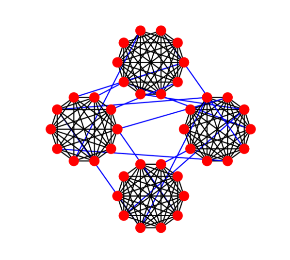
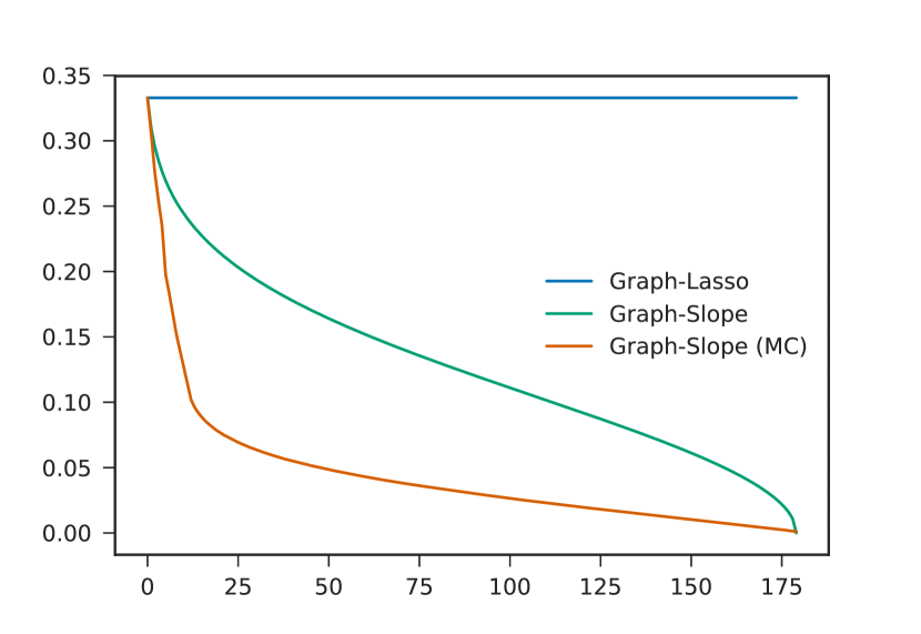
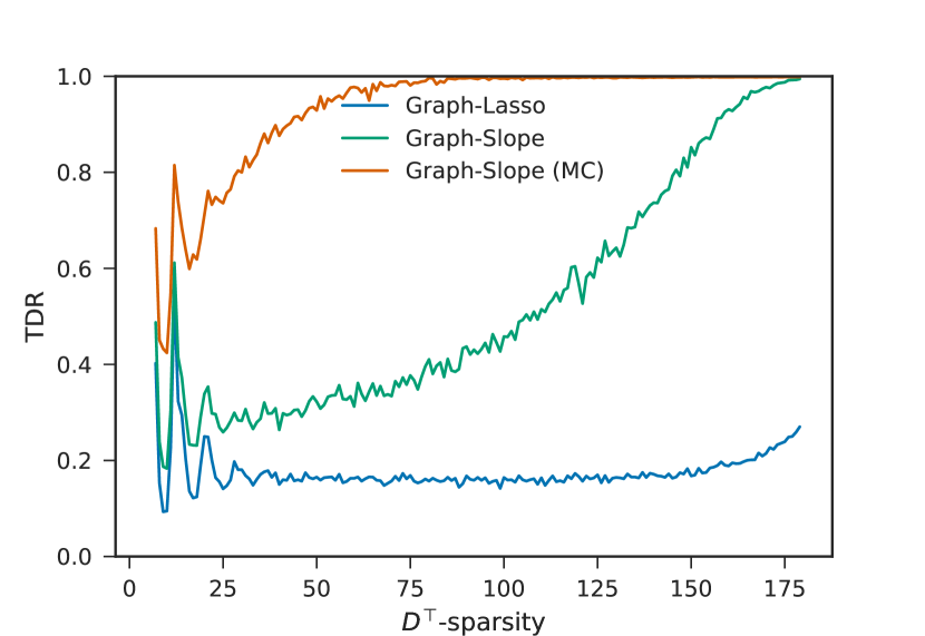
The caveman model was introduced in [34] to model small-world phenomenon in sociology. Here we consider its relaxed version, which is a graph formed by cliques of size (hence ), such that with probability , an edge of a clique is linked to a different clique. In our experiment, we set , () and . We provide a visualisation of such a graph in Figure 1(a). For this realization, we have . The rewired edges are indicated in blue in Figure 1(a) whereas the edges similar to the complete graph on 10 nodes are in black. The signals are generated as random vectors of given -sparsity with a noise level of . Figure 1(b) shows the weights decay.
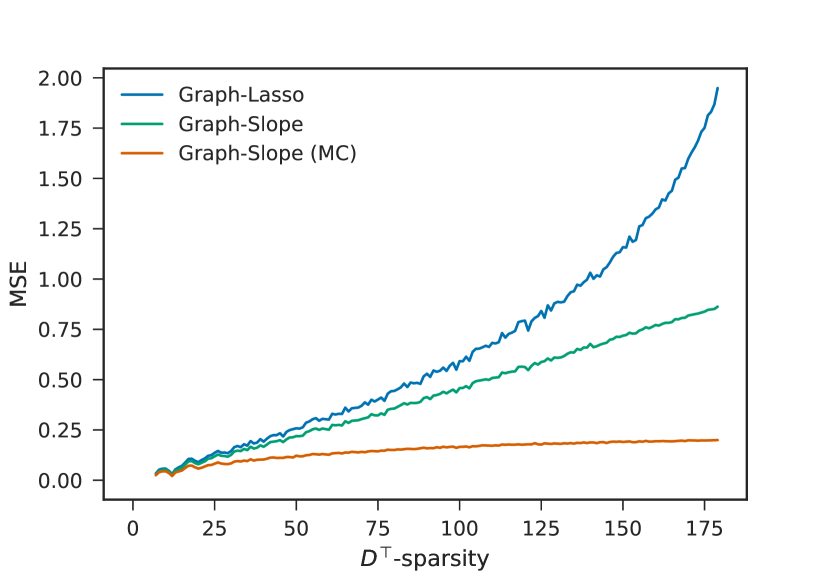
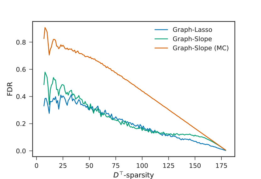
Figures 1(c)–1(e) represent the evolution of the MSE and TDR in function of the level of -sparsity. We observe that while the MSE is close between the Graph-Lasso and the Graph-Slope estimator at low level of sparsity, the TDR is vastly improved in the case of Graph-Slope, with a small price concerning the FDR (a bit more for the Monte Carlo choice of the weights). Hence empirically, Graph-Slope will make more discoveries than Graph-Lasso without impacting the overall FDR/MSE, and even improving it.
(MSE)
(FDR)
(TDR)
Example on a path: 1D–Total Variation
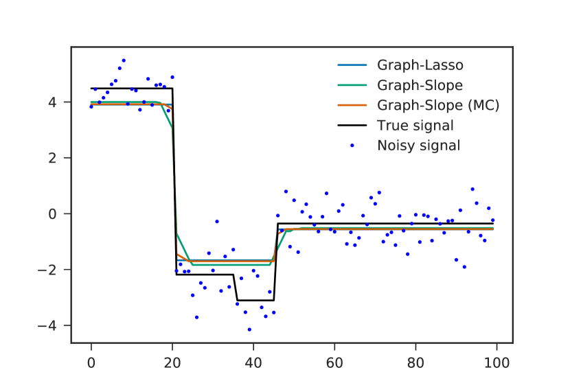
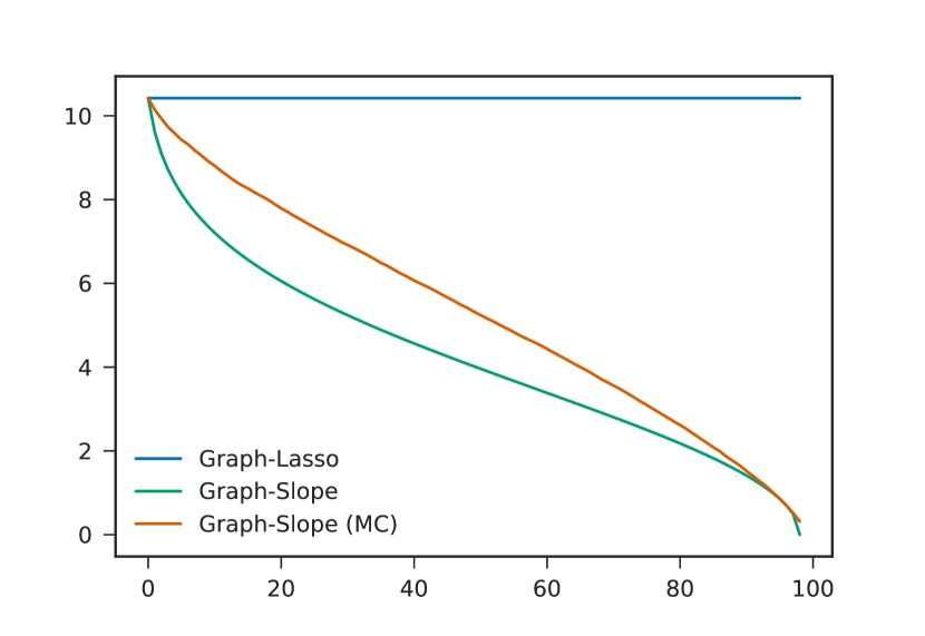
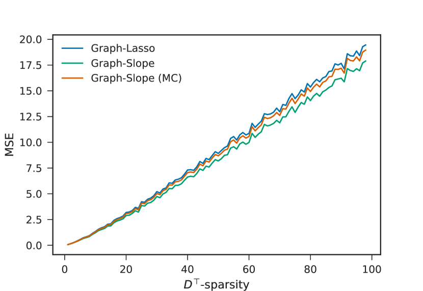
The classical 1D–Total Variation corresponds to the Graph-Lasso estimator when is the path graph over vertices, hence with edges. In our experiments, we take , and a very sparse gradient (). According to these values, and taking a random amplitude for each step, we generate a piecewise-constant signal. We display a typical realization of such a signal in Figure 2(a). Figure 2(b) shows the weights decay. Note that in this case, the Monte–Carlo weights shape differs from the one in the previous experiment. Indeed, they are adapated to the underlying graph, contrary to the theoretical weights which depend only on the size of the graph. Figures 2(c)–2(e) represent the evolution of the MSE and TDR in function of the level of -sparsity. Here, Graph-Slope does not improve the MSE significantly. However, as for the caveman experiments, Graph-Slope is more likely to make more discoveries than Graph-Lasso for a small price concerning the FDR.
(MSE)
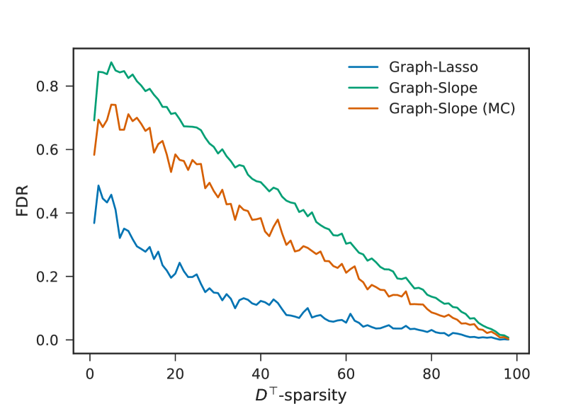
(FDR)
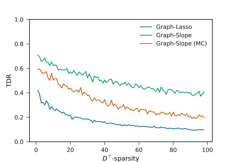
(TDR)
3.3 Example on real data: Paris roads network
To conclude our numerical experiments, we present our result on a real-life graph, the road network of Paris, France. Thanks to the Python module osmnx [9], which downloads and simplifies OpenStreetMap data, we run our experiments on streets (edges) and intersections (vertices).
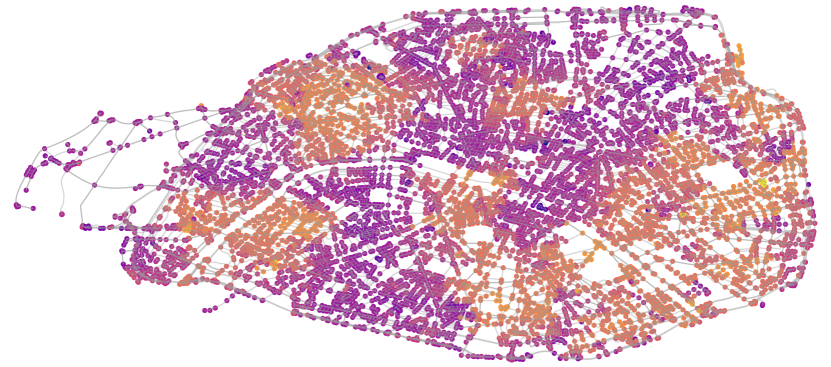
The ground truth signal is constructed as in [16] as follows. Starting from 30 infection sources, each infected intersections has probability to infect each of its neighbors. We let the infection process run for 8 iterations. The resulting graph signal is represented in Figure 3(a) with -sparsity 1586. We then corrupt this signal by a zero mean Gaussian noise with standard-deviation , leading to the observations represented in Figure 3(b).
Instead of using the parameters given in (3.11), we have computed the oracle parameters for the Graph-Lasso and Graph-Slope estimators by evaluating for 100 parameters of the form
| (3.14) |
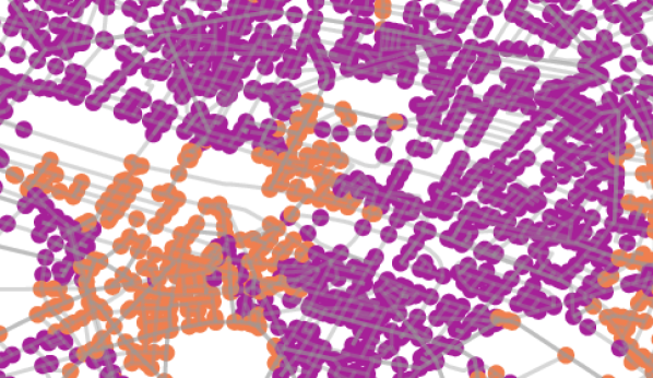
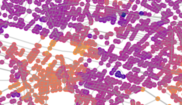
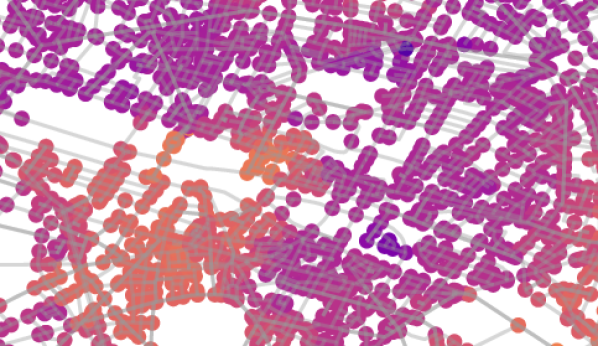
where lives on a geometric grid inside . The best one in terms of MSE (i.e., in term of ) is refered to as the oracle parameter. The results are illustrated in Figure 3(c) for Graph-Lasso and in Figure 3(d) for Graph-Slope. We can see the benefit of Graph-Slope, for instance in the center of Paris where the sources of infections are better identified as shown in the close-up, see Figures 3(e)–3(g).

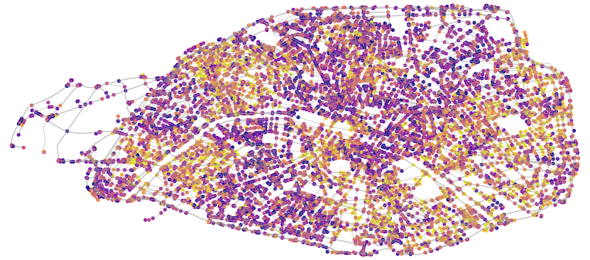
MSE=0.070,FDR=83.4%,
TDR=52.1%

MSE=0.074,FDR=88.6%,
TDR=73.5%

Appendix A Preliminary lemmas
Lemma A.1.
Let . For any two such that we have
| (A.1) |
where and .
Proof.
This is a consequence of [4, Lemma A.1]. We provide a proof here for completeness. The second inequality is simple consequence of the Cauchy-Schwarz inequality. Indeed, .
Let and and note that . Let be a permutation of such that . The first inequality can be rewritten as
| (A.2) |
where the supremum is taken over all permutations of . We now prove (A.2). Let be a permutation of such that for all . Then by the triangle inequality, we have
| (A.3) |
for each since . Furthermore, for each , it holds that so that . Thus,
| (A.4) |
It is clear that . Finally, notice that it is always possible to find a permutation such that is non-decreasing. For such choice of we have . ∎
Lemma A.2.
For the choice of weights: , the following inequalities hold true
| (A.5) |
Proof.
Reminding Stirling’s formula , one can check that
| (A.6) |
∎
Lemma A.3.
Let , , and a solution of Problem (1.7). Then, for all ,
| (A.7) |
Proof.
The objective function of the minimization problem (1.7) is the sum of two convex functions. The first term, i.e., the function , is ()-strongly convex with respect to the Euclidean norm . The sum of a 1-strongly convex function and a convex function is 1-strongly convex, and thus by multiplying by we have
| (A.8) |
for all and for any in the subdifferential of the objective function (1.7) at . Since is a minimizer of , we can choose in the above display. For , the previous display is equivalent to the claim of the Lemma. ∎
Lemma A.4.
Let us suppose that the graph has connected components . Then,
| (A.9) |
where for any , the vectors are defined by
| (A.10) |
Moreover, the orthogonal projection over is denoted by and is the component-wise averaging given by
| (A.11) |
Furthermore, if is a connected graph then .
Proof.
The proof can be done for the simple case of a connected graph (i.e., ), and the result can be generalized by tensorization of graph for components. Hence, we assume that . For any , the definition of the incidence matrix yields that for all . Since all vertices are connected, by recursion all the ’s are identical, and . The converse is proved in the same way. ∎
Lemma A.5 (Proposition E.2 in [4]).
Let be centered Gaussian random variables (not necessarily independent) with variance at most . Then,
| (A.12) |
References
- [1] I. E. Auger and C. E. Lawrence. Algorithms for the optimal identification of segment neighborhoods. Bull. Math. Biol., 51(1):39–54, 1989.
- [2] H. H. Bauschke and P. L. Combettes. Convex analysis and monotone operator theory in Hilbert spaces. Springer, New York, 2011.
- [3] A. Beck and M. Teboulle. A fast iterative shrinkage-thresholding algorithm for linear inverse problems. SIAM J. Imaging Sci., 2(1):183–202, 2009.
- [4] P. C Bellec, G. Lecué, and A. B. Tsybakov. Slope meets lasso: improved oracle bounds and optimality. arXiv preprint arXiv:1605.08651, 2016.
- [5] A. Belloni, V. Chernozhukov, and L. Wang. Square-root Lasso: pivotal recovery of sparse signals via conic programming. Biometrika, 98(4):791–806, 2011.
- [6] M. J. Best and N. Chakravarti. Active set algorithms for isotonic regression; a unifying framework. Math. Program., 47(1-3):425–439, 1990.
- [7] R. Bhatia. Matrix analysis, volume 169 of Graduate Texts in Mathematics. Springer-Verlag, New York, 1997.
- [8] P. J. Bickel, Y. Ritov, and A. B. Tsybakov. Simultaneous analysis of lasso and dantzig selector. Ann. Statist., 37(4):1705–1732, 08 2009.
- [9] G. Boeing. OSMnx: New Methods for Acquiring, Constructing, Analyzing, and Visualizing Complex Street Networks. ArXiv e-prints ArXiv:1611.01890, 2016.
- [10] M. Bogdan, E. van den Berg, C. Sabatti, W. Su, and E. J. Candès. SLOPE-adaptive variable selection via convex optimization. Ann. Appl. Stat., 9(3):1103, 2015.
- [11] S. Boucheron, G. Lugosi, and P. Massart. Concentration inequalities: A nonasymptotic theory of independence. Oxford University Press, 2013.
- [12] P. L. Combettes and J.-C. Pesquet. Proximal splitting methods in signal processing. In Fixed-point algorithms for inverse problems in science and engineering, volume 49 of Springer Optim. Appl., pages 185–212. Springer, New York, 2011.
- [13] A. S. Dalalyan, M. Hebiri, and J. Lederer. On the prediction performance of the Lasso. Bernoulli, 23(1):552–581, 2017.
- [14] C.-A. Deledalle, N. Papadakis, J. Salmon, and S. Vaiter. CLEAR: Covariant LEAst-square Re-fitting with applications to image restoration. SIAM J. Imaging Sci., 10(1):243–284, 2017.
- [15] M. Elad, P. Milanfar, and R. Rubinstein. Analysis versus synthesis in signal priors. Inverse problems, 23(3):947–968, 2007.
- [16] Z. Fan and L. Guan. -estimation of piecewise-constant signals on graphs. ArXiv e-prints ArXiv:1703.01421, 2017.
- [17] J.-C. Hütter and P. Rigollet. Optimal rates for total variation denoising. ArXiv e-prints ArXiv:1603.09388, 2016.
- [18] E. Mammen and S. van de Geer. Locally adaptive regression splines. Ann. Statist., 25(1):387–413, 1997.
- [19] E. Ndiaye, O. Fercoq, A. Gramfort, V. Leclère, and J. Salmon. Efficient smoothed concomitant lasso estimation for high dimensional regression. In NCMIP, 2017.
- [20] A. Y. Ng, M. I. Jordan, and Y. Weiss. On spectral clustering: Analysis and an algorithm. In NIPS, volume 14, pages 849–856, 2001.
- [21] A. B. Owen. A robust hybrid of lasso and ridge regression. Contemporary Mathematics, 443:59–72, 2007.
- [22] N. Parikh, S. Boyd, E. Chu, B. Peleato, and J. Eckstein. Proximal algorithms. Foundations and Trends in Machine Learning, 1(3):1–108, 2013.
- [23] F. Pedregosa, G. Varoquaux, A. Gramfort, V. Michel, B. Thirion, O. Grisel, M. Blondel, P. Prettenhofer, R. Weiss, V. Dubourg, J. Vanderplas, A. Passos, D. Cournapeau, M. Brucher, M. Perrot, and E. Duchesnay. Scikit-learn: Machine learning in Python. J. Mach. Learn. Res., 12:2825–2830, 2011.
- [24] L. I. Rudin, S. Osher, and E. Fatemi. Nonlinear total variation based noise removal algorithms. Phys. D, 60(1-4):259–268, 1992.
- [25] V. Sadhanala, Y.-X. Wang, and R. J. Tibshirani. Total variation classes beyond 1d: Minimax rates, and the limitations of linear smoothers. In NIPS, pages 3513–3521, 2016.
- [26] J. Sharpnack, A. Singh, and A. Rinaldo. Sparsistency of the edge lasso over graphs. In AISTATS, volume 22, pages 1028–1036, 2012.
- [27] J. Shi and J. Malik. Normalized cuts and image segmentation. IEEE Trans. Pattern Anal. Mach. Intell., 22(8):888–905, 2000.
- [28] W. Su and E. J. Candès. Slope is adaptive to unknown sparsity and asymptotically minimax. Ann. Statist., 44(3):1038–1068, 2016.
- [29] T. Sun and C.-H. Zhang. Scaled sparse linear regression. Biometrika, 99(4):879–898, 2012.
- [30] R. Tibshirani, M. A. Saunders, S. Rosset, J. Zhu, and K. Knight. Sparsity and smoothness via the fused LASSO. J. R. Stat. Soc. Ser. B Stat. Methodol., 67(1):91–108, 2005.
- [31] S. van de Geer and P. Bühlmann. On the conditions used to prove oracle results for the Lasso. 3:1360–1392, 2009.
- [32] V. Viallon, S. Lambert-Lacroix, H. Hoefling, and F. Picard. On the robustness of the generalized fused lasso to prior specifications. Statistics and Computing, 26(1-2):285–301, 2016.
- [33] U. Von Luxburg. A tutorial on spectral clustering. Statistics and computing, 17(4):395–416, 2007.
- [34] D. J. Watts. Networks, dynamics, and the small-world phenomenon. American Journal of Sociology, 105(2):493–527, 1999.
- [35] F. Ye and C.-H. Zhang. Rate minimaxity of the lasso and dantzig selector for the lq loss in lr balls. J. Mach. Learn. Res., 11(Dec):3519–3540, 2010.
- [36] X. Zeng and M. A. T. Figueiredo. The Ordered Weighted Norm: Atomic Formulation, Projections, and Algorithms. ArXiv e-prints arXiv:1409.4271, 2014.