Scalable Online Convolutional Sparse Coding

Abstract

Convolutional sparse coding (CSC) improves sparse coding by learning a shift-invariant dictionary from the data. However, existing CSC algorithms operate in the batch mode and are expensive, in terms of both space and time, on large data sets. In this paper, we alleviate these problems by using online learning. The key is a reformulation of the CSC objective so that convolution can be handled easily in the frequency domain and much smaller history matrices are needed. We use the alternating direction method of multipliers (ADMM) to solve the resultant optimization problem, and the ADMM subproblems have efficient closed-form solutions. Theoretical analysis shows that the learned dictionary converges to a stationary point of the optimization problem. Extensive experiments show that convergence of the proposed method is much faster and its reconstruction performance is also better. Moreover, while existing CSC algorithms can only run on a small number of images, the proposed method can handle at least ten times more images.

I Introduction

In recent years, sparse coding has been widely used in signal processing [1, 2] and computer vision [3, 4]. In sparse coding, each data sample is represented as a weighted combination of a few atoms from an over-complete dictionary learned from the data. Despite its popularity, sparse coding cannot capture shifted local patterns that are common in image samples. Often, it has to first extract overlapping image patches, which is analogous to manually convolving the dictionary with the samples. As each sample element (e.g., an image pixel) is contained in multiple overlapping patches, the separately learned representations may not be consistent. Moreover, the resultant representation is highly redundant [5].

Convolutional sparse coding (CSC) addresses this problem by learning a shift-invariant dictionary composed of many filters. Local patterns at translated positions of the samples are easily extracted by convolution, and eliminates the need for generating overlapping patches. Each sample is approximated by the sum of a set of filters convolved with the corresponding codes. The learned representations are consistent as they are obtained together. CSC has been used successfully in various image processing applications such as super-resolution image reconstruction [6], high dynamic range imaging [7], image denoising and inpainting [8]. It is also popular in biomedical applications, e.g., cell identification [9], calcium image analysis [10], tissue histology classification [11] and segmentation of curvilinear structures [12]. CSC has also been used in audio processing applications such as piano music transcription [13].

A number of approaches have been proposed to solve the optimization problem in CSC. In the pioneering deconvolutional network (DeconvNet) [14], simple gradient descent is used. As convolution is slow in the spatial domain, fast convolutional sparse coding (FCSC) [5] formulates CSC in the frequency domain, and the alternating direction method of multipliers (ADMM) [15] is used to solve the resultant optimization problem. Its most expensive operation is the inversion of a convolution-related linear operator. To alleviate this problem, convolutional basis pursuit denoising (CBPDN) [16] exploits a special structure of the dictionary, while the global consensus ADMM (CONSENSUS) [17] utilizes the matrix inverse lemma to simplify computations. Fast and flexible convolutional sparse coding (FFCSC) [8] further introduces mask matrices so as to handle incomplete samples that are common in image/video inpainting and demosaicking applications. Note that all these algorithms operate in the batch mode (i.e., all the samples/codes have to be accessed in each iteration). Hence they can become expensive, in terms of both space and time, on large data sets.

In general, online learning has been commonly used to improve the scalability of machine learning algorithms [18, 19]. While batch learning algorithms train the model after arrival of the whole data set, online learning algorithms observe the samples sequentially and update the model incrementally. Moreover, data samples need not be stored after being processed. This can significantly reduce the algorithm’s time and space complexities. In the context of sparse coding, an efficient online algorithm is proposed in [20]. In each iteration, information necessary for dictionary update is summarized in fixed-sized history matrices. The space complexity of the algorithm is thus independent of sample size. Recently, this has also been extended for large-scale matrix factorization [21].

However, though CSC is similar to sparse coding, the online sparse coding algorithm in [20] cannot be directly used. This is because convolution in CSC needs to be performed in the frequency domain for efficiency. Moreover, the sizes of history matrices depend on dimensionality of the sparse codes, which becomes much larger in CSC than in sparse coding. Storing the resultant history matrices can be computationally infeasible.

In this paper, we propose a scalable online CSC algorithm for large data sets. The algorithm, which will be called Online Convolutional Sparse Coding (OCSC), is inspired by the online sparse coding algorithm of [20]. It avoids the above-mentioned problems by reformulating the CSC objective so that convolution can be handled easily in the frequency domain and much smaller history matrices are needed. We use ADMM to solve the resultant optimization problem. It will be shown that the ADMM subproblems have efficient closed-form solutions. Consequently, to process a given number of samples, OCSC has the same time complexity as state-of-the-art batch CSC methods but requires much less space. Empirically, as OCSC updates the dictionary after coding each sample, it converges much faster than batch CSC methods. Theoretical analysis shows that the learned dictionary converges to a stationary point of the optimization problem. Extensive experiments show that convergence of the proposed method is much faster and its reconstruction performance is also better. Moreover, while existing CSC algorithms can only run on a small number of images, the proposed method can at least handle ten times more images.

The rest of the paper is organized as follows. Section II briefly reviews online sparse coding, the ADMM, and batch CSC methods. Section III describes the proposed online convolutional sparse coding algorithm. Experimental results are presented in Section IV, and the last section gives some concluding remarks.

Notations: For vector $a\in\mathbb{R}^{m}$, its $i$th element is denoted $a(i)$, its $\ell_{2}$ norm is $\|a\|_{2}=\sqrt{\sum_{i=1}^{m}a^{2}(i)}$, its $\ell_{1}$ norm is $\|a\|_{1}=\sum_{i=1}^{m}|a(i)|$, and $\text{Diag}(a)$ reshapes $a$ to a diagonal matrix with elements $a[i]$’s. Given another vector $b\in\mathbb{R}^{n}$, the convolution $a*b$ is a vector $c\in\mathbb{R}^{m+n-1}$, with $c(k)=\sum_{j=\max(1,k+1-n)}^{\min(k,m)}a(j)b(k-j+1)$. For matrix $A\in\mathbb{R}^{m\times n}$ with elements $A(i,j)$’s, $\text{vec}(A)\in\mathbb{R}^{mn}$ stacks the columns of $A$ to a vector. Given another matrix $B\in\mathbb{R}^{m\times n}$, the Hadamard product is $A\odot B=[A(i,j)B(i,j)]$. The identity matrix is denoted $I$, and the conjugate transpose is denoted $(\cdot)^{\dagger}$.

The Fourier transform that maps from the spatial domain to the frequency domain is denoted ${\cal F}$, and ${\cal F}^{-1}$ is the inverse Fourier transform. For a variable $u$ in the spatial domain, its corresponding variable in the frequency domain is denoted $\tilde{u}$.

II Related Works

II-A Online Sparse Coding

Given $N$ samples $\{x_{i},\dots,x_{N}\}$, where each $x_{i}\in\mathbb{R}^{P}$, sparse coding learns an over-complete dictionary $D\in\mathbb{R}^{P\times L}$ of $L$ atoms and sparse codes $\{z_{i}\}$ [1]. It can be formulated as the following optimization problem:

$$\min_{D\in\mathcal{D},\{z_{i}\}}\frac{1}{N}\sum_{i=1}^{N}\frac{1}{2}\|x_{i}-Dz_{i}\|^{2}_{2}+\beta\|z_{i}\|_{1},$$ (1)

where $\mathcal{D}=\{D:\left\|D(:,l)\right\|_{2}\leq 1\text{ for $l=1,\dots,L$}\}$ and $\beta\geq 0$. Many efficient algorithms have been developed for solving (1). Examples include K-SVD [1] and active set method [2]. However, they require storing all the samples, which can become infeasible when $N$ is large.

To solve this problem, an online learning algorithm for sparse coding that processes samples one at a time is proposed in [20]. After observing the $t$th sample $x_{t}$, the sparse code $z_{t}$ is obtained as

$$z_{t}=\arg\min_{z}\frac{1}{2}\|x_{t}-D_{t-1}z\|^{2}_{2}+\beta\|z\|_{1},$$ (2)

where $D_{t-1}$ is the dictionary obtained at the $(t-1)$th iteration. After obtaining $z_{t}$, $D_{t}$ is updated as

$$D_{t} = \arg\min_{D\in\mathcal{D}}\frac{1}{t}\sum_{i=1}^{t}\frac{1}{2}\|x_{i}-Dz_{i}\|^{2}_{2}+\beta\|z_{i}\|_{1}$$ (3)

$$= \arg\min_{D\in\mathcal{D}}\text{tr}(D^{\top}DA_{t}^{\text{(osc)}}-2D^{\top}B_{t}^{\text{(osc)}}),$$ (4)

where

$$A_{t}^{\text{(osc)}} = \frac{1}{t}\sum_{i=1}^{t}z_{i}z_{i}^{\top}\in\mathbb{R}^{L\times L},$$ (5)

$$B_{t}^{\text{(osc)}} = \frac{1}{t}\sum_{i=1}^{t}x_{i}z_{i}^{\top}\in\mathbb{R}^{P\times L}.$$ (6)

Each column $D_{t}(:,l)$ in (4) can be obtained by coordinate descent. $A_{t}^{\text{(osc)}}$ and $B_{t}^{\text{(osc)}}$ can also be updated incrementally as

$$A_{t}^{\text{(osc)}} = \frac{t-1}{t}A_{t-1}^{\text{(osc})}+\frac{1}{t}z_{i}z_{i}^{\top},$$

$$B_{t}^{\text{(osc)}} = \frac{t-1}{t}B_{t-1}^{\text{(osc)}}+\frac{1}{t}x_{i}z_{i}^{\top}.$$ (7)

Using $A_{t}^{\text{(osc)}}$ and $B_{t}^{\text{(osc)}}$, one does not need to store all the samples and codes to update $D_{t}$. The whole algorithm is shown in Algorithm 1.

Algorithm 1 Online sparse coding [20].

0:  samples $\{x_{i}\}$.

1:  Initialize: dictionary $D_{0}$ as a Gaussian random matrix, $A_{0}^{\text{(osc)}}=\mathbf{0}$, $B_{0}^{\text{(osc)}}=\mathbf{0}$;

2:  for $t=1,2,\dots,T$ do

3:     draw $x_{t}$ from $\{x_{i}\}$;

4:     obtain sparse code $z_{t}$ using (2);

5:     update history matrices $A_{t}^{\text{(osc)}},B_{t}^{\text{(osc)}}$ using (7);

6:     update dictionary $D_{t}$ using (4) by coordinate descent;

7:  end for

8:  return  $D_{T}$.

The following assumptions are made in [20].

Assumption 1.

1. Samples $\{x_{i}\}$ are generated i.i.d. from some distribution with $\|x_{i}\|_{2}$ bounded.

2. The code $z_{t}$ is unique w.r.t. data $x_{t}$.

3. The objective in (4) is strictly convex with lower-bounded Hessians.

Theorem 1 ([20]).

With Assumption 1, the distance between $D_{t}$ and the set of stationary points of the dictionary learning problem converges almost surely to 0 when $t\rightarrow\infty$.

II-B Alternating Direction Method of Multipliers (ADMM)

ADMM [15] has been popularly used for solving optimization problems of the form

$$\min_{x,y}\;f(x)+g(y)\;:\;Ax+By=c,$$ (8)

where $f,g$ are convex functions, and $A,B$ (resp. $c$) are constant matrices (resp. vector). It first constructs the augmented Lagrangian of problem (8)

$$f(x)+g(y)+\nu^{\top}(Ax+By-c)+\frac{\rho}{2}\|Ax+By-c\|^{2},$$ (9)

where $\nu$ is the dual variable, and $\rho>0$ is a penalty parameter.

At the $\tau$th iteration, the values of $x$ and $y$ (denoted as $x_{\tau}$ and $y_{\tau}$) are updated by minimizing (9) w.r.t. $x$ and $y$ in an alternating manner. Define the scaled dual variable $u_{\tau}={\nu_{\tau}}/\rho$. The ADMM updates can be written as

$$x_{\tau} =\arg\min_{x}f(x)+\frac{\rho}{2}\|Ax+By_{\tau-1}-c+u_{\tau-1}\|_{2}^{2},$$

$$y_{\tau} =\arg\min_{y}g(y)+\frac{\rho}{2}\|Ax_{\tau}+By-c+u_{\tau-1}\|_{2}^{2},$$ (10)

$$u_{\tau} =u_{\tau-1}+Ax_{\tau}+By_{\tau}-c.$$ (11)

The above procedure converges to the optimal solution at a rate of $O(1/T)$ [22], where $T$ is the number of iterations.

II-C Convolutional Sparse Coding

Convolutional sparse coding (CSC) learns a dictionary $D\in\mathbb{R}^{M\times K}$ composed of $K$ filters, each of length $M$, that can capture the same local pattern at different translated positions of the samples. This is achieved by replacing the multiplication between dictionary and code by convolution. While each $x_{i}$ in sparse coding is represented by a single code $z_{i}\in\mathbb{R}^{K}$, each $x_{i}$ in CSC is represented by $K$ codes stored together in the matrix $Z_{i}\in\mathbb{R}^{P\times K}$.

The dictionary and codes are obtained by solving the following optimization problem:

$$\min_{D\in\mathcal{D},\{Z_{i}\}}\!\frac{1}{N}\!\sum_{i=1}^{N}\!\frac{1}{2}\|x_{i}\!-\!\sum_{k=1}^{K}D(:,k)\!*\!Z_{i}(:,k)\|^{2}_{2}+\beta\|Z_{i}\|_{1},\!$$ (12)

where $*$ denotes convolution in the spatial domain.

Convolution can be accelerated in the frequency domain via the convolution theorem [23]: $\mathcal{F}({D}(:,k)*{Z}(:,k))=\mathcal{F}({D}(:,k))\odot\mathcal{F}({Z}(:,k))$, where ${D}(:,k)$ is first zero-padded to $P$-dimensional. Hence, recent CSC methods [5, 8, 16, 17] choose to operate in the frequency domain. Let $\tilde{x}_{i}\equiv\mathcal{F}(x_{i})$, $\tilde{D}(:,k)\equiv\mathcal{F}(D(:,k))$ and $\tilde{Z}_{i}(:,k)\equiv\mathcal{F}(Z_{i}(:,k))$. (12) is reformulated as

$$\min_{\tilde{D},\{\tilde{Z}_{i}\}} \frac{1}{N}\sum_{i=1}^{N}\frac{1}{2P}\|\tilde{x}_{i}-\sum_{k=1}^{K}\tilde{D}(:,k)\odot\tilde{Z}_{i}(:,k)\|^{2}_{2}+\beta\sum_{k=1}^{K}\|\mathcal{F}^{-1}(\tilde{Z}_{i}(:,k))\|_{1}\!\!$$

s.t. $$\|\mathcal{H}(\mathcal{F}^{-1}(\tilde{D}(:,k)))\|_{2}^{2}\leq 1,k=1,\dots,K,$$

where the factor $\frac{1}{P}$ in the objective comes from the Parseval’s theorem [24], and $\mathcal{H}$ is the linear operation that removes the extra $P-M$ dimensions in $\mathcal{F}^{-1}(\tilde{D}(:,k))$.

Problem (II-C) can be solved by block coordinate descent [5, 8, 16, 17], which updates $\{\tilde{Z}_{i}\}$ and $\tilde{D}$ alternately.

II-C1 Updating $\{\tilde{Z}_{i}\}$

Given $\tilde{D}$, the $\{\tilde{Z}_{i}\}$ can be obtained one by one for each $i$th sample as

$$\min_{\tilde{Z}_{i},{U}_{i}} ~{}~{}\frac{1}{2P}\|\tilde{x}_{i}\!-\!\sum_{k=1}^{K}\tilde{D}(:,k)\odot\tilde{Z}_{i}(:,k)\|^{2}_{2}+\beta\|U_{i}\|_{1}$$ (13)

s.t. $$~{}~{}U_{i}(:,k)=\mathcal{F}^{-1}(\tilde{Z}_{i}(:,k)),\;k=1,\dots,K,$$

where $U_{i}$ is introduced to decouple the loss and the $\ell_{1}$-regularizer in (II-C). This can then be solved by ADMM [5, 8, 16, 17].

II-C2 Updating $\tilde{D}$

Given $\{\tilde{Z}_{i}\}$, $\tilde{D}$ can be obtained as

$$\min_{\tilde{D},V} \frac{1}{2NP}\sum_{i=1}^{N}\|\tilde{x}_{i}-\sum_{k=1}^{K}\tilde{D}(:,k)\odot\tilde{Z}_{i}(:,k)\|^{2}_{2}$$ (14)

s.t. $$\begin{cases}\mathcal{F}(V(:,k))=\tilde{D}(:,k),&k=1,\dots,K,\\ \|\mathcal{H}((V(:,k)))\|_{2}^{2}\leq 1,&k=1,\dots,K,\end{cases}$$

where $V$ is introduced to decouple the loss and constraint in (II-C). This can again be solved by using ADMM [5, 8, 16, 17].

After obtaining $\{\tilde{Z}_{i}\}$ and $\tilde{D}$, the sparse codes can be recovered as $Z_{i}(:,k)=\mathcal{F}^{-1}(\tilde{Z}_{i}(:,k))$ for $i=1,\dots,N$, and the dictionary filters as $D(:,k)=\mathcal{H}(\mathcal{F}^{-1}(\tilde{D}(:,k)))$.

The above algorithms all need $O(NPK)$ in space. They differ mainly in how to compute the linear system involved with $\tilde{D}$ in the ADMM subproblems. FCSC [5] directly solves the subproblem, which takes $O(NK^{3}P)$ time. CBPDN [16] exploits a special structure in the dictionary and reduces the time complexity to $O(N^{2}KP)$, which is efficient for small $N$. The CONSENSUS algorithm [17] utilizes the matrix inverse lemma to reduce the time complexity to $O(NKP^{2})$. The state-of-the-art is FFCSC [8], which incorporates various linear algebra techniques (such as Cholesky factorization [25] and cached factorization [25]) to reduce the time complexity to $O(NK^{2}P)$.

III Online Convolutional Sparse Coding

Existing CSC algorithms operate in the batch mode, and need to store all the samples and codes which cost $O(NPK)$ space. This becomes infeasible when the data set is large. In this section, we will scale up CSC by using online learning.

After observing the $t$th sample $x_{t}$, online CSC considers the following optimization problem which is analogous to (12):

$$\min_{D\in\mathcal{D},\{Z_{i}\}}\frac{1}{t}\sum_{i=1}^{t}\frac{1}{2}\|x_{i}\!-\!\sum_{k=1}^{K}D(:,k)*Z_{i}(:,k)\|^{2}_{2}+\beta\|Z_{i}\|_{1}.$$ (15)

To solve problem (15), some naive approaches are first considered in Section III-A. The proposed online convolutional sparse coding algorithm is then presented in Section III-B. It takes the same time complexity for one data pass as state-of-the-art batch CSC algorithms, but has a much lower space complexity (Section III-C). The convergence properties of the proposed algorithm is discussed in Section III-D.

III-A Naive Approaches

As in batch CSC, problem (15) can be solved by alternating minimization w.r.t. the codes and dictionary (as in Section II-C). Given the dictionary, the codes are updated as in (13). Given the codes, the dictionary is updated by solving the following optimization subproblem analogous to (14):

$$\min_{\tilde{D},V} \frac{1}{2tP}\sum_{i=1}^{t}\|\tilde{x}_{i}-\sum_{k=1}^{K}\tilde{D}(:,k)\odot\tilde{Z}_{i}(:,k)\|^{2}_{2}$$ (16)

s.t. $$\begin{cases}\mathcal{F}(V(:,k))=\tilde{D}(:,k),&k=1,\dots,K,\\ \|\mathcal{H}(V(:,k))\|_{2}^{2}\leq 1,&k=1,\dots,K.\end{cases}$$

However, solving (16) as in Section II-C2 requires keeping all the samples and codes, and is computationally expensive on large data sets.

Alternatively, the objective in (16) can be rewritten as

$$\frac{1}{2tP}\sum_{i=1}^{t}\left\|\tilde{x}_{i}\!-\!\dot{D}\dot{z}_{i}\right\|^{2}_{2},$$ (17)

where

$$\dot{D}=[\text{Diag}(\tilde{D}(:,1)),\dots,\text{Diag}(\tilde{D}(:,K))],$$ (18)

and $\dot{z}_{i}=\text{vec}(\tilde{Z}_{i})$. This is of the form in (3). Hence, we may attempt to reuse the online sparse coding in Algorithm 1, and thus avoid storing all the samples and codes. However, recall that online learning the dictionary is possible because one can summarize the observed samples into the history matrices $A_{t}^{\text{(osc)}},B_{t}^{\text{(osc)}}$ in (5), (6). For (17), the history matrices become

$${A}_{t}^{\text{(naive)}} = \frac{1}{t}\sum_{i=1}^{t}\dot{z}_{i}\dot{z}_{i}^{\dagger}\in\mathbb{R}^{PK\times PK},$$ (19)

$${B}_{t}^{\text{(naive)}} = \frac{1}{t}\sum_{i=1}^{t}\tilde{x}_{i}\dot{z}_{i}^{\dagger}\in\mathbb{R}^{P\times PK}.$$

In typical CSC applications, the number of image pixels $P$ is at least in the tens of thousands, and $N$ may only be in the thousands. Hence, the $O(K^{2}P^{2})$ space required for storing ${A}_{t}^{\text{(naive)}}$ and ${B}_{t}^{\text{(naive)}}$ is even higher than the $O(NKP)$ space required for batch methods.

III-B Proposed Algorithm

Note that $\dot{D}$ in (18) is composed of a number of diagonal matrices. By utilizing this special structure, the following Proposition rewrites the objective in (16) so that much smaller history matrices can be used.

Proposition 2.

The objective in (16) is equivalent to the following apart from a constant:

$$\frac{1}{2P}\sum_{p=1}^{P}\tilde{D}(p,:)\left(\frac{1}{t}\sum_{i=1}^{t}\tilde{Z}_{i}^{\dagger}(:,p)\tilde{Z}_{i}(p,:)\right)\tilde{D}^{\dagger}(:,p)-\frac{1}{P}\sum_{p=1}^{P}\tilde{D}(p,:)\left(\frac{1}{t}\sum_{i=1}^{t}\tilde{x}_{i}(p)\tilde{Z}_{i}^{\dagger}(:,p)\right),$$ (20)

The proof is in Appendix A-A. Obviously, each $\tilde{D}(p,:)$ in (20) can then be independently optimized. This avoids directly handling the much larger $P\times PK$ matrix $\dot{D}$ in (18). Let

$${A}^{p}_{t} = \frac{1}{t}\sum_{i=1}^{t}\tilde{Z}_{i}^{\dagger}(:,p)\tilde{Z}_{i}(p,:)\in\mathbb{R}^{K\times K},$$

$${b}^{p}_{t} = \frac{1}{t}\sum_{i=1}^{t}\tilde{x}_{i}(p)\tilde{Z}_{i}^{\dagger}(:，p)\in\mathbb{R}^{K}$$

in (20). The total space required for $\{{A}^{p}_{t},{b}^{p}_{t}\}$ is $O(K^{2}P)$, which is much smaller than the $O(K^{2}P^{2})$ space for storing ${A}_{t}^{\text{(naive)}}$ in (19). Moreover, as in (7), ${A}^{p}_{t}$ and ${b}^{p}_{t}$ can be updated incrementally as

$${A}^{p}_{t} =\left(1-\frac{1}{t}\right){A}^{p}_{t-1}+\frac{1}{t}\tilde{Z}_{t}^{\dagger}(:,p)\tilde{Z}_{t}(p,:),$$ (21)

$${b}^{p}_{t} =\left(1-\frac{1}{t}\right){b}^{p}_{t-1}+\frac{1}{t}\tilde{x}_{t}(p)\tilde{Z}_{t}^{\dagger}(:，p).$$ (22)

The dictionary and codes can then be efficiently updated in an alternating manner as follows.

III-B1 Updating the Dictionary

With the codes fixed, using Proposition 2, the dictionary can be updated by solving the following optimization problem:

$$(\tilde{D}_{t},V_{t}) =\arg\min_{\tilde{D},V}\frac{1}{2P}\sum_{p=1}^{P}\!\!\tilde{D}(p,:){A}^{p}_{t}\tilde{D}^{\dagger}(:,p)\!-\!2\tilde{D}(p,:){b}^{p}_{t}$$ (23)

$$\text{s.t.}\;\mathcal{F}(V(:,k))=\tilde{D}(:,k),k=1,\dots,K,\quad\|\mathcal{H}(V(:,k))\|_{2}^{2}\leq 1,k=1,\dots,K.$$

This can solved using ADMM. At the $\tau$th ADMM iteration, let $\Theta_{t,\tau}$ be the ADMM dual variable. The following shows the update equations for $\tilde{D}$ and $V$.

Updating $\tilde{D}_{t,\tau}$: From (20), $\tilde{D}_{t,\tau}$ can be updated by solving the following subproblem:

$$\tilde{D}_{t,\tau}=\arg\min_{\tilde{D}}\frac{1}{2P}\sum_{p=1}^{P}\tilde{D}(p,:){A}^{p}_{t}\tilde{D}^{\dagger}(:,p)-2\tilde{D}(p,:){b}^{p}_{t}+\frac{\rho}{2}\sum_{k=1}^{K}\|\tilde{D}(:,k)-\tilde{V}_{t,\tau-1}(:,k)+\Theta_{t,\tau-1}(:,k)\|_{2}^{2},$$

where $\tilde{V}_{t,\tau-1}(:,k)\equiv\mathcal{F}({V}_{t,\tau-1}(:,k))$. Note that $\|\tilde{D}\|_{F}^{2}=\sum_{p=1}^{P}\|\tilde{D}(p,:)\|_{2}^{2}=\sum_{k=1}^{K}\|\tilde{D}(:,k)\|_{2}^{2}$. Hence, $\sum_{k=1}^{K}\|\tilde{D}(:,k)-\tilde{V}_{t,\tau-1}(:,k)+\Theta_{t,\tau-1}(:,k)\|_{2}^{2}=\sum_{p=1}^{P}\|\tilde{D}(p,:)-\tilde{V}_{t,\tau-1}(p,:)+\Theta_{t,\tau-1}(p,:)\|_{2}^{2}$. The rows of $\tilde{D}_{t,\tau}$ can then be obtained separately as

$$\tilde{D}_{t,\tau}(p,:)\!\!\!\! = \!\!\!\!\min_{\tilde{D}(p,:)}\frac{1}{2P}(\tilde{D}(p,:){A}^{p}_{t}\tilde{D}^{\dagger}(:,p)-2\tilde{D}(p,:){b}^{p}_{t})+\frac{\rho}{2}\|\tilde{D}(p,:)-\tilde{V}_{t,\tau-1}(p,:)+\Theta_{t,\tau-1}(p,:)\|_{2}^{2}$$ (24)

$$= \!\!\!\!({b}^{p\dagger}_{t}\!+\!\rho P\tilde{V}_{t,\tau-1}(p,:)\!-\!\rho P\Theta_{t,\tau-1}(p,:)){C}^{p}_{t},$$

where ${C}^{p}_{t}=({A}^{p}_{t}+\rho PI)^{-1}$. With $\{C^{p}_{t}\}$, we do not need to store $\{A^{p}_{t}\}$.

Computing the matrix inverse ${C}^{p}_{t}\in\mathbb{C}^{K\times K}$ takes $O(K^{3})$ time. This can be simplified by noting from (21) that ${A}^{p}_{t}+\rho PI$ is the sum of rank-1 matrices and a (scaled) identity matrix. Using the Sherman-Morrison formula [25], we have

$${C}^{p}_{t}=\left\{\begin{array}[]{ll}\frac{1}{\rho P}I-\frac{1}{\rho P}\frac{\tilde{Z}_{t}^{\dagger}(:,p)\tilde{Z}_{t}(p,:)}{\rho P+\tilde{Z}_{t}(p,:)\tilde{Z}_{t}^{\dagger}(:,p)}&t=1\\ \frac{t}{t-1}\left[{C}^{p}_{t-1}-\frac{{C}^{p}_{t-1}\tilde{Z}_{t}^{\dagger}(:,p)\tilde{Z}_{t}(p,:){C}^{p}_{t-1}}{(t-1)+\tilde{Z}_{t}(p,:){C}^{p}_{t-1}\tilde{Z}_{t}^{\dagger}(:,p)}\right]&t>1\end{array}\right..$$ (25)

This takes $O(K^{2})$, instead of $O(K^{3})$, time.

Updating $V_{t,\tau}$: From (10), each column $V_{t,\tau}(:,k)$ can be updated as

$$\min_{V(:,k)}\frac{\rho}{2}\|\tilde{D}_{t,\tau}(:,k)\!-\!\mathcal{F}(V(:,k))\!+\!\Theta_{t,\tau-1}(:,k)\|_{2}^{2},\quad\text{s.t.}\|\mathcal{H}(V(:,k))\|_{2}^{2}\leq 1.$$

It has the following closed-form solution.

Proposition 3 ([29]).

$V_{t,\tau}(:,k)=\alpha/\max(\|\alpha\|_{2},1)$, where $\alpha=\mathcal{H}(\mathcal{F}^{-1}(\tilde{D}_{t,\tau}(:,k)+\Theta_{t,\tau-1}(:,k)))$.

Finally, the dual variables $\Theta_{t,\tau}$ is updated as in (11). The whole dictionary update procedure (DictOCSC) is shown in Algorithm 2. As (23) is convex, convergence to the globally optimal solution is guaranteed [22].

Algorithm 2 DictOCSC($\tilde{D}_{t-1},\{b^{p}_{t}\},\{C^{p}_{t}\}$).

0:  initial dictionary $\tilde{D}_{t-1}$, $\{{b}^{p}_{t}\}$, $\{{C}^{p}_{t}\}$;

1:  Initialize: $\tilde{D}_{t,0}=\tilde{D}_{t-1}$, $V_{t,0}=\mathbf{0}$, $\Theta_{t,0}=\mathbf{0}$;

2:  for $\tau=1,2,\dots,J$ do

3:     update $\{\tilde{D}_{t,\tau}(1,:),\dots,\tilde{D}_{t,\tau}(P,:)\}$ using (24);

4:     update $\{V_{t,\tau}(:,1),\dots,V_{t,\tau}(:,K)\}$ using Proposition 3;

5:     update $\{\Theta_{t,\tau}(:,1),\dots,\Theta_{t,\tau}(:,K)\}$ as $\Theta_{t,\tau}(:,k)=\Theta_{t,\tau-1}(:,k)+\tilde{D}_{t,\tau}(:,k)-\mathcal{F}(V_{t,\tau}(:,k))$;

6:  end for

7:  return  $\tilde{D}_{t,J}$.

In batch CSC methods, its dictionary update in (14) is also based on ADMM (Section II-C2). However, our dictionary update step first reformulates the objective as in (20). This enables each ADMM subproblem to be solved with a much lower space complexity ($O(K^{2}P)$ vs $O(NKP)$ for the state-of-the-art [8]) but still with the same iteration time complexity (i.e., $O(NK^{2}P+NKP\log P)$).

III-B2 Updating the Code

Given the dictionary, as the codes for different samples are independent, they can be updated one by one as in batch CSC methods (Section II-C1).

The whole algorithm, which will be called Online Convolutional Sparse Coding (OCSC), is shown in Algorithm 3.

Algorithm 3 Online convolutional sparse coding (OCSC).

0:  samples $\{x_{i}\}$.

1:  Initialize: dictionary $\tilde{D}_{0}$ as a Gaussian random matrix, $\{{C}_{0}^{p}\}=\mathbf{0}$, $\{{b}_{0}^{p}\}=\mathbf{0}$;

2:  for $t=1,2,\dots,T$ do

3:     $\tilde{x}_{t}=\mathcal{F}(x_{t})$, where $x_{t}$ is drawn from $\{x_{i}\}$;

4:     obtain $\tilde{Z}_{t}$ using (13);

5:     update $\{{b}^{1}_{t},\dots,{b}^{P}_{t}\}$ using (22);

6:     update $\{{C}^{1}_{t},\dots,{C}^{P}_{t}\}$ using (25);

7:     $\tilde{D}_{t}=\text{DictOCSC}(\tilde{D}_{t-1},\{b^{p}_{t}\},\{C^{p}_{t}\})$.

8:  end for

9:  for $k=1,2,\dots,K$ do

10:     $D_{T}(:,k)=\mathcal{H}(\mathcal{F}^{-1}(\tilde{D}_{T}(:,k)))$;

11:  end for

12:  return  $D_{T}$.

III-C Complexity Analysis

In Algorithm 3, the space requirement is dominated by $\{C^{p}_{t}\}$, which takes $O(K^{2}P)$ space. For one data pass which precesses $N$ samples, updating $\{C^{p}_{t}\}$ and $\{b^{p}_{t}\}$ takes $O(NK^{2}P)$ time, dictionary update takes $O(NK^{2}P)$ time, code update takes $O(NKP)$ time, and FFT/inverse FFT takes $O(NKP\log P)$ time. Hence, one data pass takes a total of $O(NK^{2}P+NKP\log P)$ time.

A comparison with the existing batch CSC algorithms is shown in Table I. As can be seen, the proposed algorithm takes the same time complexity for one data pass as the state-of-the-art FFCSC algorithm, but has a much lower space complexity ($O(K^{2}P)$ instead of $O(NKP)$).

TABLE I: Comparing the proposed online CSC algorithm with existing batch CSC algorithms.

	batch/online	convolution operation	space	time for one data pass
DeconvNet [14]	batch	spatial	$O(NKP)$	$O(NK^{2}P^{2}M)$
FCSC [5]	batch	frequency	$O(NKP)$	$O(NK^{3}P+NKP\log P)$
FFCSC [8]	batch	frequency	$O(NKP)$	$O(NK^{2}P+NKP\log P)$
CBPDN [16]	batch	frequency	$O(NKP)$	$O(N^{2}KP+NKP\log P)$
CONSENSUS [17]	batch	frequency	$O(NKP)$	$O(NKP^{2}+NKP\log P)$
OCSC	online	frequency	$O(K^{2}P)$	$O(NK^{2}P+NKP\log P)$

III-D Convergence

In this section, we show that Algorithm 3 outputs a stationary point of the CSC problem (15) when $t\rightarrow\infty$. This is achieved by connecting Algorithm 3 to a direct application of Algorithm 1 on (15).

The convolution operation in the spatial domain can be written as matrix multiplication [5, 14]. Specifically,

$$D(:,k)*Z(:,k)=\mathcal{T}(D(:,k))Z(:,k),$$ (26)

where $\mathcal{T}(x)$ is a linear operator which maps a vector to its associated Toeplitz matrix. Specifically,

$$\mathcal{T}(D(:,k))=\left[\begin{array}[]{ccccc}D(1,k)&0&0&&D(2,k)\\ D(2,k)&D(1,k)&0&\ddots&D(3,k)\\ D(3,k)&D(2,k)&D(1,k)&&D(4,k)\\ \vdots&\vdots&\vdots&\ddots&\vdots\\ D(M,k)&D(M-1,k)]&D(M-2,k)&&\\ 0&D(M,k)&D(M-1,k)&&\\ \vdots&\vdots&\vdots&\ddots&\vdots\\ 0&0&0&&D(1,k)\end{array}\right].$$

The number of columns in $\mathcal{T}(D(:,k))$ is equal to the dimension of $Z(:,k)$ (i.e., $P$).

Let $\bar{D}_{k}=\mathcal{T}(D(:,k))\in\mathbb{R}^{P\times P}$, $\mathcal{T}^{-1}$ be the inverse operator of $\mathcal{T}$ which maps $\bar{D}_{k}$ back to $D(:,k)$, $\bar{D}=\left[\bar{D}_{1},\dots,\bar{D}_{K}\right]$ and $\bar{z}_{i}=\text{vec}(Z_{i})$. Problem (15) can be rewritten as

$$\min_{\bar{D}\in\mathcal{S},\{\bar{z}_{i}\}}\frac{1}{t}\sum_{i=1}^{t}\frac{1}{2}\|x_{i}-\bar{D}\bar{z}_{i}\|^{2}_{2}+\beta\|\bar{z}_{i}\|_{1},$$ (28)

where

$$\mathcal{S}=\left\{\bar{D}_{k}:\|\mathcal{T}^{-1}(\bar{D}_{k})\|_{2}^{2}\leq 1\right\}.$$ (29)

Thus, the objective (28) is of the same form as that in (3). However, a direct use of Algorithm 1 is not feasible. First, the feasible region $\mathcal{S}$ in (29) is more complex, and coordinate descent cannot be used as there is no simple projection to $\mathcal{S}$. Second, as $\bar{z}_{i}$ is of length $KP$, the corresponding history matrices (analogous to those in (5)) require $O(K^{2}P^{2})$ space.

Though a direct application of Algorithm 1 is not practical, Theorem 1 still holds. Indeed, Theorem 1 can be further extended by relaxing its feasible region $\mathcal{C}$ on $D$. As discussed in [20], $\mathcal{C}$ can be, for example, $\{D:\|D(:,l)\|_{2}\leq 1\;\text{and}\;D(i,j)\geq 0\}$. It is mentioned in [20] that $\mathcal{C}$ has to be a union of independent constraints on each column of $D$. However, this only serves to facilitate the use of coordinate descent (step 6 in Algorithm 1), but is not required in the proof. In general, Theorem 1 holds when $\mathcal{C}$ is bounded, convex, and $\mathcal{C}\subseteq\mathcal{D}$.

The following Lemma shows that $\mathcal{S}$ in (29) satisfies the conditions. The proof is in Appendix A-B. Thus, Theorem 1 also holds for Algorithm 3, and a stationary point of problem (15) can be obtained.

Lemma 4.

$\mathcal{S}$ in (29) is bounded, convex, and a subset of $\mathcal{D}$.

III-E Discussion with [27, 28]

Here, we discuss the very recent works of [27, 28] which also consider online learning of the dictionary in CSC. Extra experiments are performed in Section B, which shows our method is much faster than them.

In the online convolutional dictionary learning (OCDL) algorithm [27], convolution is performed in the spatial domain. They started with the observation that convolution is commutative. Hence, for the summation $\sum_{k=1}^{K}D(:,k)*Z_{i}(:,k)$ in (15), we have

$$\sum_{k=1}^{K}D(:,k)*Z_{i}(:,k)=\sum_{k=1}^{K}Z_{i}(:,k)*D(:,k)=\sum_{k=1}^{K}\mathcal{T}(Z_{i}(:,k))D(:,k)=\bar{Z}_{i}\bar{d},$$ (30)

where $\bar{Z}_{i}=\left[\mathcal{T}(Z_{i}(:,1)),\dots,\mathcal{T}(Z_{i}(:,K))\right]$ with $\mathcal{T}(Z_{i}(:,k))\in\mathbb{R}^{P\times M}$ and $\bar{d}=\text{vec}(D)$. (15) can then be rewritten as

$$\min_{\bar{d},\{\bar{Z}_{i}\}}\frac{1}{2t}\sum_{i=1}^{t}\left\|{x}_{i}-\bar{Z}_{i}\bar{d}\right\|^{2}_{2}+\lambda\|\bar{Z}_{i}\|_{1}\quad\text{s.t.}\quad\|D(:,k)\|_{2}^{2}\leq 1,k=1,\dots,K,$$ (31)

where $\lambda=\beta/P$ (as each $Z_{i}(:,k)$ is repeated $P$ times in the Toeplitz matrix $\bar{Z}_{i}$). Using (31), the history matrices are constructed as

$${A}_{t}^{\text{(ocdl1)}} = \frac{1}{t}\sum_{i=1}^{t}\bar{Z}_{i}^{\top}\bar{Z}_{i}\in\mathbb{R}^{KM\times KM},$$

$${b}_{t}^{\text{(ocdl1)}} = \frac{1}{t}\sum_{i=1}^{t}\bar{Z}_{i}^{\top}x_{i}\in\mathbb{R}^{KM}.$$

Recall that $M$ is the length of filter $D(:,k)$ when CSC is solved in the spatial domain. The space complexity of [27] is dominated by $\bar{Z}_{i}$ (which takes $O(KPM)$ space) or ${A}_{t}^{\text{(ocdl1)}}$ (which takes $O(K^{2}M^{2})$ space), depending on the relative sizes of $P$ and $KM$. Though this is comparable to our $O(K^{2}P)$ space requirement, its time complexity is much larger. For one data pass, convolution in the spatial domain takes $O(NKPM)$ time and updating the history matrices above takes $O(NK^{2}PM^{2})$ time. The dictionary update in total takes $O(NK^{2}PM^{2}+NKPM)$ time. In contrast, the proposed algorithm takes $O(NK^{2}P+NKP\log P)$ time. In the experiments, $M=11\times 11$, and $P$ ranges from $32\times 32$ to $500\times 500$. Thus, the algorithm in [27] is much more expensive.

The algorithm in [28], also called online convolutional dictionary learning, considers the frequency domain and solves problem (16) as in the proposed method. First, they rewrite (16) as

$$\min_{\dot{d},\{\dot{Z}_{i}\}}\frac{1}{2tP}\sum_{i=1}^{t}\left\|\tilde{x}_{i}-\dot{Z}_{i}\dot{d}\right\|^{2}_{2}+\beta\|\dot{Z}_{i}\|_{1}\quad\text{s.t.}\quad\|\mathcal{H}(\mathcal{F}^{-1}(\tilde{D}(:,k)))\|_{2}^{2}\leq 1,k=1,\dots,K,$$

where $\dot{Z}_{i}=[\text{Diag}(\tilde{Z}_{i}(:,1)),\dots,\text{Diag}(\tilde{Z}_{i}(:,K))]$, and $\dot{d}=\text{vec}(\tilde{D})$. The history matrices are then constructed as

$${A}_{t}^{\text{(ocdl2)}} = \frac{1}{t}\sum_{i=1}^{t}\dot{Z}_{i}^{\top}\dot{Z}_{i}\in\mathbb{R}^{KP\times KP},$$

$${b}_{t}^{\text{(ocdl2)}} = \frac{1}{t}\sum_{i=1}^{t}\dot{Z}_{i}^{\top}\tilde{x}_{i}\in\mathbb{R}^{KP}.$$

They proposed to store ${A}_{t}^{\text{(ocdl2)}}$ and the history matrices in sparse format. These take $O(K^{2}P)$ space, and is the same as our $\{C^{p}_{t}\}$ in (25) which are stored in dense format. However, though their $O(\cdot)$ are the same, storing sparse matrix requires 2-3 times more space than storing dense matrix with the same number of nonzero entries, as each nonzero entry in a sparse matrix needs to be kept in the compressed sparse row (CSR) format [30]. Moreover, though [28] and the proposed method take $O(NK^{2}P)$ time to update the history matrices, using sparse matrices as in [28] is empirically slower [30]. Preliminary experiments show that with $K=100$ filters, the proposed algorithm is $5$ times faster on an $P=100\times 100$ image and $10$ times faster on an $P=200\times 200$ image.

Moreover, we use ADMM for optimization, while [27, 28] use the FISTA algorithm [31]. Empirically, ADMM has been shown to be faster than FISTA on solving the CSC problem [16]. We also empirically verify this point in Section B-B.

IV Experiments

In this section, experiments are performed on six image data sets (Table II). The Fruit, City and House data sets are standard benchmarks in CSC [5, 8, 14]. However, they are relatively small. Hence, we include three larger data sets: (i) Flower, which contains images from 102 flower categories [32]; (ii) Dog, which contains images of 120 breeds of dogs [33]; and (iii) CIFAR-10, which contains images from 10 general object classes [34]. The training images are used to learn the dictionary, which is then used to reconstruct the test set images. We use the default training and test splits provided. The images are preprocessed as in [8, 14]. We convert each image to grayscale, and perform local contrast normalization. Edge-tapering is used to blur the edges of the samples with a random Gaussian filter.

TABLE II: Summary of data sets used.

	dimension ($P$)	#training images	#testing images
Fruit	100$\times$100	10	4
City	100$\times$100	10	4
House	100$\times$100	100	4
Flower	500$\times$500	2040	6149
Dog	224$\times$224	12000	8580
CIFAR-10	32$\times$32	50000	10000

The proposed OCSC is compared with the following (batch) CSC methods:

1. Deconvolutional networks (DeconvNet) [14];

2. Fast convolutional sparse coding (FCSC) [5];

3. Fast and flexible convolutional sparse coding (FFCSC) [8];

4. Convolutional basis pursuit denoising (CBPDN) [16];

5. The global consensus ADMM (CONSENSUS) algorithm [17].

All the codes are in Matlab and obtained from the respective authors (except FCSC). We do not compare with [27, 28], as their codes are not publicly available.

We follow the hyperparameter setting in [8], and set $\beta=1$, $M=11$ and $K=100$. The batch methods are stopped when the relative changes in $\{Z_{i}\}$ (i.e., $\frac{1}{N}\sum_{i=1}^{N}\|Z_{i}-Z_{i}^{\text{old}}\|_{2}/\|Z_{i}\|_{2}$) and $D$ (i.e., $\|D-D^{\text{old}}\|_{2}/\|D\|_{2}$) are both smaller than ${10}^{-3}$. As for the proposed online method, it is stopped when the relative changes in $Z_{t}$ (i.e., $\|Z_{t}-Z_{t}^{\text{old}}\|_{2}/\|Z_{t}\|_{2}$) and $D$ (i.e., $\|D-D^{\text{old}}\|_{2}/\|D\|_{2}$) are both smaller than ${10}^{-3}$. Experiments are run on a PC with Intel i7 4GHz CPU with 32GB memory.

To compare the empirical convergence of various methods, we monitor the test set objective as in [20, 21]. This is obtained as

$$\min_{\{Z_{i}\}}\frac{1}{|\Omega|}\sum_{x_{i}\in\Omega}\frac{1}{2}\|x_{i}-\sum_{k=1}^{K}D_{t}(:,k)*Z_{i}(:,k)\|^{2}_{2}+\beta\|Z_{i}\|_{1},$$

where $\Omega$ is the test set, and $D_{t}$ is the dictionary learned after the $t$th data pass. As for image reconstruction quality, we use the peak signal-to-noise ratio on the test set [8]:

$$\text{PSNR}=\frac{1}{|\Omega|}\sum_{x_{i}\in\Omega}10\log_{10}\left(\frac{255^{2}P}{\|{x}^{\text{rec}}_{i}-{x}_{i}\|_{2}^{2}}\right),$$

where ${x}^{\text{rec}}_{i}=\sum_{k=1}^{K}D_{T}(:,k)*Z_{i}(:,k)$ is the reconstructed image for $x_{i}$ by using the final dictionary $D_{T}$. To reduce statistical variability, we repeat the experiment five times by using different dictionary initializations and orders to present images to the algorithm. The PSNR is then averaged over these five repetitions.

IV-A Small Data Sets

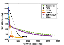
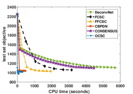
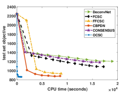
In this section, we perform experiments on the small data sets (Fruit, City and House). Figure 1 shows the test set objective vs CPU time. Though FFCSC has the same time complexity as OCSC, OCSC is still much faster. This is because batch CSC methods update the dictionary only after coding all the samples, while OCSC can refine the dictionary after coding each sample. A similar behavior is also observed between online and batch SC methods [20].

Table III compares the image reconstruction performance. As OCSC converges to a lower objective than its batch counterparts (Figure 1), it also outperforms the others in terms of image reconstruction quality. Among all methods, OCSC performs the best, which is then followed by CBPDN, FCSC and FFCSC. CONSENSUS and DeconvNet perform the worst.

(a) Fruit.

(b) City.

(c) House.

Figure 1: Test set objective vs CPU time on the small data sets.

TABLE III: Testing PSNR obtained on the small data sets. The highest and comparable PSNR (according to the pairwise t-test with 95% confidence) are in bold.

	Fruit	City	House
DeconvNet	27.41$\pm$0.13	28.11$\pm$0.25	25.39$\pm$0.27
FCSC	27.90$\pm$0.18	28.20$\pm$0.31	25.68$\pm$0.50
FFCSC	28.13$\pm$0.15	28.58$\pm$0.16	28.48$\pm$0.04
CBPDN	28.01$\pm$0.04	28.67$\pm$0.37	29.40$\pm$0.43
CONSENSUS	27.62$\pm$0.14	28.19$\pm$0.20	25.41$\pm$0.37
OCSC	28.61$\pm$0.06	28.86$\pm$0.13	29.68$\pm$0.06

Figure 2 shows the difference between the reconstructed images and the corresponding ground truths of some sample test set images from the Fruit data set. As can be seen, the images reconstructed by OCSC are most similar to the ground truths, which is then followed by CBPDN, FFCSC and FCSC. Images reconstructed by CONSENSUS and DeconvNet are the least similar to the ground truths. A similar observation is also observed on City and House, which are not reported here because of the lack of space.

(a) Ground truth.

(b) DeconvNet.

(c) FCSC.

(d) FFCSC.

(e) CBPDN.

(f) CONSENSUS.

(g) OCSC.

Figure 2: Differences between the ground truth and reconstruction on test set images of the Fruit data set.

(a) DeconvNet.

(b) FCSC.

(c) FFCSC.

(d) CBPDN.

(e) CONSENSUS.

(f) OCSC.

Figure 3: Dictionaries learned on the Fruit data set.

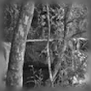
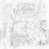
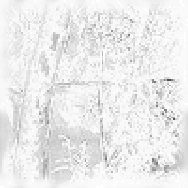
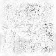
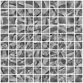
Figure 3 shows the dictionaries learned on Fruit (results on City and House are similar). As in [1], the filters are sorted in ascending order of the variance. As can be seen, dictionaries learned by FCSC, FFCSC, CBPDN and OCSC contain Gabor-style filters, while the dictionaries learned by DeconvNet and CONSENSUS are vague. We speculate that this is due to slow convergence of these two methods, as observed in Figure 1.

(a) Flower.

(b) Dog.

(c) CIFAR-10.

Figure 4: Testing PSNR with varying number of training images.

(a) Flower.

(b) Dog.

(c) CIFAR-10.

Figure 5: CPU time with varying number of training images.

IV-B Large Data Sets

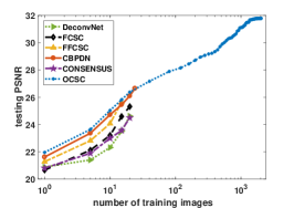
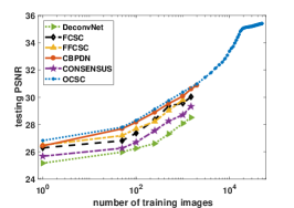
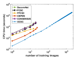
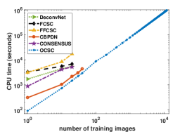
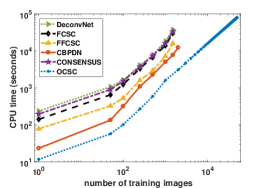
As discussed in Section III-C, the space complexity of OCSC is independent of $N$. Hence, it can handle much larger training image sets than batch CSC methods. In this section, we illustrate this on the Flower, Dog and CIFAR-10 data sets. The Flower images are large ($500\times 500$), and the batch CSC methods quickly run out of memory. To allow comparison with the batch methods, we use $K$ as 50.

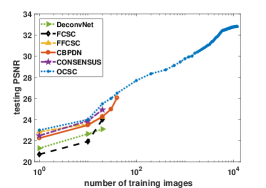
Figure 4(a) shows the testing PSNR with varying number of training images on the Flower data set. As can be seen, performance is improved with more training images. However, the batch CSC methods run out of memory quickly. Specifically, CBPDN can only handle 25 training images, while the other batch methods can only handle 20. Figures 4(b) and 4(c) show results on Dog and CIFAR-10, respectively. Among the batch methods, CBPDN can handle 40 training images on Dog and 2000 training images on CIFAR-10, while the others can only handle 20 training images on Dog and 1500 training images on CIFAR-10. On the other hand, OCSC can always handle the full training data set.

Figure 5 shows the CPU time with different numbers of training images. Given the same amount of time, OCSC can train on more images than the batch methods. Combined with Figure 4, OCSC obtains higher testing PSNR than batch methods given the same amount of time.

V Conclusion

In this paper, we proposed a scalable convolutional sparse coding methods in the online setting. By reformulating the CSC objective, the sizes of the history matrices required in the online setup can be significantly reduced. Moreover, the resultant optimization problem can be efficiently solved using ADMM, with closed-form solutions for the ADMM subproblems. We also provide theoretical guarantee on the convergence of the proposed algorithm. While the batch CSC methods need large space and heavy computation cost, extensive experiments show that the proposed method can efficiently learn from large data sets with much less space.

As for future work, we will consider introducing nonconvex regularizers to CSC. Traditionally, the convex $\ell_{1}$-regularizer is used to encourage sparsity among the codes. Though this leads to easier optimization, the resultant code may not be as sparse and accurate as when a nonconvex regularizer (such as the log-sum-penalty) is used [35]. Moreover, on large data sets, many filters are often needed to capture the presence of more local patterns. Though the proposed online algorithm has reduced the space consumption significantly compared to batch CSC methods, its space complexity still depends on the number of filters. A promising direction is to further reduce the storage by approximating the filters as linear combinations of a few base filters.

Appendix A Proofs

A-A Proposition 2

Proof.

(17) can be expanded as

$$\arg\min_{\tilde{D}}\frac{1}{2tP}\sum_{i=1}^{t}\left\|\tilde{x}_{i}-\dot{D}\dot{z}_{i}\right\|^{2}_{2}=\arg\min_{\tilde{D}}\frac{1}{2P}\text{tr}\left(\dot{D}^{\dagger}\dot{D}\left(\sum_{i=1}^{t}\frac{1}{t}\dot{z}_{i}\dot{z}_{i}^{\dagger}\right)-2\dot{D}^{\dagger}\left(\sum_{i=1}^{t}\frac{1}{t}\tilde{x}_{i}\dot{z}_{i}^{\dagger}\right)\right),$$

where $\dot{D}=[\text{Diag}(\tilde{D}(:,1)),\dots,\text{Diag}(\tilde{D}(:,K))]$, and $\dot{z}_{i}=\text{vec}(\tilde{Z}_{i})$. Thus,

$$\dot{D}^{\dagger}\dot{D}\!\!\! = \!\!\!\left[\begin{array}[]{c}\begin{smallmatrix}\tilde{D}(1,1)&&0\\ &\ddots&\\ 0&&\tilde{D}(P,1)\rule[-3.01389pt]{0.0pt}{6.02777pt}\end{smallmatrix}\\ \ddots\\ \begin{smallmatrix}\rule{0.0pt}{6.02777pt}\tilde{D}(1,K)&&0\\ &\ddots&\\ 0&&\tilde{D}(P,K)\end{smallmatrix}\end{array}\right]\cdot\left[\begin{array}[]{ccc}\begin{smallmatrix}\tilde{D}(1,1)&&0\\ &\ddots&\\ 0&&\tilde{D}(P,1)\rule[-3.01389pt]{0.0pt}{6.02777pt}\end{smallmatrix}\ddots\begin{smallmatrix}\rule{0.0pt}{6.02777pt}\tilde{D}(1,K)&&0\\ &\ddots&\\ 0&&\tilde{D}(P,K)\end{smallmatrix}\end{array}\right].$$

For $\tilde{D}(j,k)$, only when it is multiplied by elements of the same row index $\tilde{D}(j,l)$, $l=1,\dots,K$, will result in non-zero values. In other words, multiplications among different rows can be avoided. We then directly operate on each row of $\dot{D}$, which is exactly $\tilde{D}(p,:)$ if zeros are dropped. Consequently, we have the form in Proposition 2. ∎

A-B Lemma 4

Proof.

Obviously, $\mathcal{S}$ is a convex constraint set. To show $\mathcal{S}\subset\mathcal{D}$, recall that $\bar{D}=[T(D(:,1)),\dots,T(D(:,K))]$, where each $T(D(:,k))$ is the Toeplitz matrix associated with $D_{t}(:,k)$ as defined in (26). Because of the constraint $\|D(:,k)\|_{2}^{2}\leq 1$, each column $\bar{D}(:,l)$ of $\bar{D}$, satisfies $\|\bar{D}(:,l)\|_{2}^{2}\leq 1$. Thus $\|\bar{D}\|_{F}^{2}\leq KP$. Hence, $\mathcal{S}\subset\mathcal{D}$ and $\mathcal{S}$ is bounded. ∎

Appendix B Experimental Comparison with [27, 28]

In this section, we provide extra experimental results comparing OCSC with concurrent works OCDL1 [27] and OCDL2 [28] discussed in Section III-E. We use implementation by ourself as no pubic codes are available.

B-A Large Data Sets

We experiment on large data sets to test these online methods’ scalability. The evaluation metric used on empirical convergence is test set objective, on image reconstruction quality is PSNR. CIFAR-10 is used, which has a large number of small images ($P=32\times 32$). This is because a single image of Flower ($P=500\times 500$) makes both OCDL1 and OCDL2 run out of memory, even Dog ($P=224\times 224$) makes OCDL2 not work. Hence for complete comparison, we use CIFAR-10 only.

We still use the same training and test splits as in Section IV. Hyper-parameters are the same as Section IV. As a recap, we set $\beta=1$, $M=11$ and $K=100$. The methods are stopped when the relative changes in $Z_{t}$ (i.e., $\|Z_{t}-Z_{t}^{\text{old}}\|_{2}/\|Z_{t}\|_{2}$) and $D$ (i.e., $\|D-D^{\text{old}}\|_{2}/\|D\|_{2}$) are both smaller than ${10}^{-3}$.

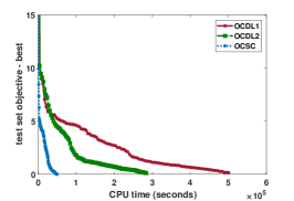
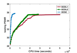
Figure 6(a) shows the test set objective vs CPU time. As shown, OCSC converges the fastest, then OCDL2 follows, OCDL1 is the slowest. OCDL1 lags behinds due to its slow convolution performed in spatial domain and the costly updating of history matrices. As for OCDL2, although it shares the efficiency of performing convolution in frequency domain, it is very slow to deal with sparse matrices. They finally reach to comparable testing objective value as they are solving the same online CSC problem. Figure 6(b) shows the testing PSNR vs CPU time. For all three methods, the testing PSNR is improved given more training images, and they can reach similar final testing PSNR. However, the CPU time needed to reach it varies a lot. In other words, given same amount of time, OCSC always gets a higher testing PSNR.

(a) CPU time v.s testing objective.

(b) CPU time v.s testing PSNR.

Figure 6: Comparison with OCDL1 [27] and OCDL2 [28] on CIFAR-10 dataset.

B-B Synthetic Data

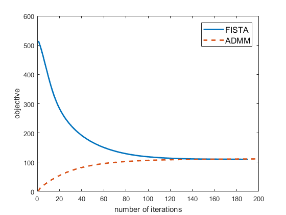
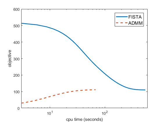
In this section, we perform experiments on synthetic data to compare the convergence speed of ADMM (used by our OCSC) and FISTA (used by both OCDL1 [27] and OCDL2 [28]) on CSC problem. We evaluate the convergence speed by training set objective vs time. We choose frequency domain to compare the efficiency of ADMM and FISTA. As shown in Figure 6(a) and Figure 6(b), although OCDL1 and OCDL2 both use FISTA, OCDL1 which operates in spatial domain is much slower than OCDL2 which operates in frequency domain. Specifically, we compare proposed ADMM on (23) with FISTA on (III-E) [28]. Note that the two problems are equivalent to (16), thus we compute the objective based on (16).

We set $K=100$, and the size of synthetic data $x\in\mathbb{R}^{P}$ where $P=10000$. The entries of $x$, $D$ and $Z$ are sampled i.i.d. from the standard normal distribution $\mathcal{N}(0,1)$, and each $D(:,:,k),k=1\dots K$ is projected to the $\ell_{2}$-norm unit ball.

The comparison of objective vs iterations and CPU time are shown in Figure 7(a) and Figure 7(b). In terms of the number of iterations, ADMM converges faster than FISTA. Then, in terms of time, FISTA is much slower than ADMM. This relates to the design of OCDL2 mentioned in [28]. Empirically, for our data, OCDL2’s history matrices need hundreds of GBs in dense format. Hence to fit into memory, OCDL2 has to operate on sparse matrices, which is much slower on matrix multiplications. This also verifies our discussion in Section III-E, ADMM converges faster than FISTA on CSC problem.

(a) Objective v.s number of iterations.

(b) Objective v.s CPU time (seconds).

Figure 7: Comparison of FISTA and ADMM on the synthetic data.

References

- [1] M. Aharon, M. Elad, and A. Bruckstein, “K-SVD: An algorithm for designing overcomplete dictionaries for sparse representation,” IEEE Transactions on Signal Processing, vol. 54, no. 11, pp. 4311–4322, Nov. 2006.
- [2] H. Lee, A. Battle, R. Raina, and A. Ng, “Efficient sparse coding algorithms,” in Advances in Neural Information Processing Systems, 2007, pp. 801–808.
- [3] J. Mairal, F. Bach, J. Ponce, G. Sapiro, and A. Zisserman, “Non-local sparse models for image restoration,” in International Conference on Computer Vision, 2009, pp. 2272–2279.
- [4] J. Yang, K. Yu, Y. Gong, and T. Huang, “Linear spatial pyramid matching using sparse coding for image classification,” in IEEE Conference on Computer Vision and Pattern Recognition, 2009, pp. 1794–1801.
- [5] H. Bristow, A. Eriksson, and S. Lucey, “Fast convolutional sparse coding,” in IEEE Conference on Computer Vision and Pattern Recognition, 2013, pp. 391–398.
- [6] S. Gu, W. Zuo, Q. Xie, D. Meng, X. Feng, and L. Zhang, “Convolutional sparse coding for image super-resolution,” in International Conference on Computer Vision, 2015, pp. 1823–1831.
- [7] A. Serrano, F. Heide, D. Gutierrez, G. Wetzstein, and B. Masia, “Convolutional sparse coding for high dynamic range imaging,” in Computer Graphics Forum, vol. 35, no. 2, 2016, pp. 153–163.
- [8] F. Heide, W. Heidrich, and G. Wetzstein, “Fast and flexible convolutional sparse coding,” in IEEE Conference on Computer Vision and Pattern Recognition, 2015, pp. 5135–5143.
- [9] M. Pachitariu, A. Packer, N. Pettit, H. Dalgleish, M. Hausser, and M. Sahani, “Extracting regions of interest from biological images with convolutional sparse block coding,” in Advances in Neural Information Processing Systems, 2013, pp. 1745–1753.
- [10] F. Andilla and F. Hamprecht, “Sparse space-time deconvolution for calcium image analysis,” in Advances in Neural Information Processing Systems, 2014, pp. 64–72.
- [11] H. Chang, J. Han, C. Zhong, A. Snijders, and J. Mao, “Unsupervised transfer learning via multi-scale convolutional sparse coding for biomedical applications,” IEEE Transactions on Pattern Analysis and Machine Intelligence, 2017.
- [12] R. Annunziata and E. Trucco, “Accelerating convolutional sparse coding for curvilinear structures segmentation by refining SCIRD-TS filter banks,” IEEE Transactions on Medical Imaging, vol. 35, no. 11, pp. 2381–2392, Nov. 2016.
- [13] A. Cogliati, Z. Duan, and B. Wohlberg, “Context-dependent piano music transcription with convolutional sparse coding,” IEEE/ACM Transactions on Audio Speech and Language Processing, vol. 24, no. 12, pp. 2218–2230, Dec. 2016.
- [14] M. Zeiler, D. Krishnan, G. Taylor, and R. Fergus, “Deconvolutional networks,” in IEEE Conference on Computer Vision and Pattern Recognition, 2010, pp. 2528–2535.
- [15] S. Boyd, N. Parikh, E. Chu, B. Peleato, and J. Eckstein, “Distributed optimization and statistical learning via the alternating direction method of multipliers,” Foundations and Trends in Machine Learning, vol. 3, no. 1, pp. 1–122, 2011.
- [16] B. Wohlberg, “Efficient algorithms for convolutional sparse representations,” IEEE Transactions on Image Processing, vol. 25, no. 1, pp. 301–315, Jan. 2016.
- [17] M. Šorel and F. Šroubek, “Fast convolutional sparse coding using matrix inversion lemma,” Digital Signal Processing, vol. 55, pp. 44–51, Aug. 2016.
- [18] N. Cesa-Bianchi and G. Lugosi, Prediction, Learning, and Games. Cambridge University Press, 2006.
- [19] S. Shalev-Shwartz, “Online learning and online convex optimization,” Foundations and Trends in Machine Learning, vol. 4, no. 2, pp. 107–194, 2012.
- [20] J. Mairal, F. Bach, J. Ponce, and G. Sapiro, “Online learning for matrix factorization and sparse coding,” Journal of Machine Learning Research, vol. 11, pp. 19–60, Jan. 2010.
- [21] A. Mensch, J. Mairal, B. Thirion, and G. Varoquaux, “Dictionary learning for massive matrix factorization,” in International Conference on Machine Learning, 2016, pp. 1737–1746.
- [22] B. He and X. Yuan, “On the convergence rate of the Douglas-Rachford alternating direction method,” SIAM Journal on Numerical Analysis, vol. 50, no. 2, pp. 700–709, Jan. 2012.
- [23] S. Mallat, A Wavelet Tour of Signal Processing. Academic Press, 1999.
- [24] W. Chew, Waves and Fields in Inhomogeneous Media. New York: IEEE, 1995, vol. 522.
- [25] A. Jennings and J. McKeown, Matrix Computation. John Wiley & Sons, 1992.
- [26] Y. Wang, Q. Yao, J. T. Kwok, and L. M. Ni, “Online convolutional sparse coding,” Preprint arXiv:1706.06972, 2017.
- [27] K. Degraux, U. S. Kamilov, P. T. Boufounos, and D. Liu, “Online convolutional dictionary learning for multimodal imaging,” arXiv preprint arXiv:1706.04256, 2017.
- [28] J. Liu, C. Garcia-Cardona, B. Wohlberg, and W. Yin, “Online convolutional dictionary learning,” arXiv preprint arXiv:1709.00106, 2017.
- [29] N. Parikh and S. Boyd, “Proximal algorithms,” Foundations and Trends in Optimization, vol. 1, no. 3, pp. 127–239, 2014.
- [30] T. A. Davis, Direct Methods for Sparse Linear Systems. SIAM, Jan. 2006.
- [31] A. Beck and M. Teboulle, “A fast iterative shrinkage-thresholding algorithm for linear inverse problems,” SIAM Journal on Imaging Sciences, vol. 2, no. 1, pp. 183–202, Jan. 2009.
- [32] M. Nilsback and A. Zisserman, “Automated flower classification over a large number of classes,” in Indian Conference on Computer Vision, Graphics & Image Processing, 2008, pp. 722–729.
- [33] A. Khosla, N. Jayadevaprakash, B. Yao, and F. Li, “Novel dataset for fine-grained image categorization,” in Workshop on Fine-Grained Visual Categorization, 2011.
- [34] A. Krizhevsky and G. Hinton, “Learning multiple layers of features from tiny images,” University of Toronto, Tech. Rep., 2009.
- [35] E. Candès, M. Wakin, and S. Boyd, “Enhancing sparsity by reweighted minimization,” Journal of Fourier Analysis and Applications, vol. 14, no. 5-6, pp. 877–905, Dec. 2008.