Lumping of Degree-Based Mean-Field and Pair Approximation Equations
for Multi-State Contact Processes

Charalampos Kyriakopoulos1    Gerrit Grossmann1    Verena Wolf1    Luca Bortolussi2 1Computer Science Department, Saarland University 2Department of Mathematics and Geosciences, University of Trieste
Abstract

Contact processes form a large and highly interesting class of dynamic processes on networks, including epidemic and information spreading networks. While devising stochastic models of such processes is relatively easy, analyzing them is very challenging from a computational point of view, particularly for large networks appearing in real applications. One strategy to reduce the complexity of their analysis is to rely on approximations, often in terms of a set of differential equations capturing the evolution of a random node, distinguishing nodes with different topological contexts (i.e., different degrees of different neighborhoods), such as degree-based mean-field (DBMF), approximate master equation (AME), or pair approximation (PA) approaches. The number of differential equations so obtained is typically proportional to the maximum degree kmaxsubscript𝑘maxk_{\mathrm{max}} of the network, which is much smaller than the size of the master equation of the underlying stochastic model, yet numerically solving these equations can still be problematic for large kmaxsubscript𝑘maxk_{\mathrm{max}}. In this paper, we consider AME and PA, extended to cope with multiple local states, and we provide an aggregation procedure that clusters together nodes having similar degrees, treating those in the same cluster as indistinguishable, thus reducing the number of equations while preserving an accurate description of global observables of interest. We also provide an automatic way to build such equations and to identify a small number of degree clusters that give accurate results. The method is tested on several case studies, where it shows a high level of compression and a reduction of computational time of several orders of magnitude for large networks, with minimal loss in accuracy.

pacs:
Valid PACS appear here
preprint: APS/123-QED

I Introduction

Dynamic processes on complex networks have attracted a lot of interest in recent years Albert and Barabási (2002); Newman (2003); Strogatz (2001); Palla et al. (2005); Boccaletti et al. (2006); Barrat et al. (2008); Dorogovtsev et al. (2008); Pastor-Satorras et al. (2015). Their behavior is complex and their dynamics is strongly influenced by the network topology through interactions between connected nodes. Even more challenging is the study of adaptive networks, where both the node state and the network topology coevolve in a feedback relationship Gross et al. (2006); Gross and Blasius (2008); Marceau et al. (2010); Van Segbroeck et al. (2010); Wu et al. (2012); Wang et al. (2015).

Among dynamic processes happening on networks, a prominent role is played by contact processes, which include information spreading and epidemic models Barrat et al. (2008); Mata et al. (2014); Gómez et al. (2011); Juhász et al. (2012); Boguñá et al. (2009); Lee et al. (2013); Pastor-Satorras et al. (2015). In a contact process, each node of the network can be in one of several states, and neighboring nodes can interact and change their state. Interactions typically happen at random times, governed by an exponential distribution. The underlying stochastic process is therefore a discrete-state Markov jump process.

The analysis of such models is very challenging, because of the huge state space of the underlying process: each possible network configuration (i.e., each assignment of states to nodes) represents a different discrete (global) state of the process. The exponential blowup of the state space rules out the use of any numerical technique to compute probabilities, such as uniformization or finite projection methods Didier et al. (2009); Wolf et al. (2010), but also renders simulation quite expensive, particularly for very large networks. An alternative and viable approach for large networks is provided by mean-field-like approximations Bortolussi et al. (2013). There are several forms and variations of such approximations Pastor-Satorras and Vespignani (2001); Gleeson (2011); Cator and Van Mieghem (2012); Mata and Ferreira (2013); Demirel et al. (2014); Pastor-Satorras et al. (2015) for network models, all sharing the same basic idea, namely to treat all nodes with a similar local structure as indistinguishable, and write a differential equation for each class of nodes, modeling the evolution of a random node in time. Depending on how much information about the local structure is taken into account, we obtain more refined approximations, at the price of more equations to be solved. In the simplest case, we treat all nodes with the same local state as indistinguishable (mean-field (MF) approximation Bortolussi et al. (2013); Barrat et al. (2008)). Improvements can be obtained by grouping nodes with respect to their state and degree, called degree-based (described also as heterogeneous sometimes) mean-field (DBMF) Pastor-Satorras and Vespignani (2001); Castellano and Pastor-Satorras (2010); Gleeson et al. (2012), while an even better approximation is achieved by also representing explicitly also the state of neighboring nodes, as introduced by Gleeson’s approximate master equation (AME) for the binary state case Gleeson (2011). By implicitly relying on a binomial assumption, these equations can be simplified to yield the pair approximation (PA) Gleeson (2011). Although for many network topologies AME and PA give significantly more accurate results Gleeson (2013), solving the AME and PA, even for the binary state case considered by Gleeson, is much more expensive than DBMF.

For the general multi-state case that we consider here, the solution of AME and PA is usually infeasible for many real networks, as we show that the number of equations is (kmax+|S||S|1)(kmax+1)binomialsubscript𝑘max𝑆𝑆1subscript𝑘max1\binom{k_{\mathrm{max}}+|S|}{|S|-1}(k_{\mathrm{max}}+1) for AME and (|S|2+|S|)kmaxsuperscript𝑆2𝑆subscript𝑘max(|S|^{2}+|S|)k_{\mathrm{max}} for PA, where kmaxsubscript𝑘maxk_{\mathrm{max}} is the maximum degree of the network and |S|𝑆|S| is the number of possible states of a node.

Typically, when analyzing dynamic processes on complex networks, the interest is in emergent behaviors that manifest at a collective level. Hence, aggregated quantities like the fraction of nodes in a certain state are typically monitored. However, the network topology, even if marginalized in such observables, highly influences their dynamic properties. Often, the necessary granularity of the analysis is on the level of DBMF or PA. Here, we show that the level of detail of these approaches can be further decreased. Our lumping approach shows that for an accurate approximation of the mean behavior of the nodes, the exact degree and state of the neighborhood need not be monitored. Instead, aggregated information is sufficient, which strongly lowers the complexity of the analysis. We decrease the number of equations by several orders of magnitude without noticable loss in precision compared to PA or DBMF. Moreover, we are able to set up an automatic procedure to construct such compressed equations, which avoids altogether the solution of the full system of equations. Computational gains are impressive, up to five orders of magnitude for large networks (large kmaxsubscript𝑘maxk_{\mathrm{max}}). This increased performance can be extremely useful when equations have to be solved many times, for instance for parameter sweeping or for parameter identification tasks.

In this paper, we consider AME and PA for the case of |S|𝑆|S| local states, providing explicitly the AME and the derivation of PA in a similar fashion as in Fennell (2015). For the special case of contact processes, we arrive at an equation that involves the first and second moments of the multinomial distribution, which renders the equations computationally more tractable compared to Fennell (2015).

Our major contributions are the following: (i) we derive a lumped set of equations for the multi-state DBMF and PA equations and propose an algorithm to effectively construct this set; and (ii) we provide a numerical study on several non-trivial examples, showing that our approach performs well for several classes of degree distributions, that the reduction becomes more and more effective as the maximum network degree increases, and that non-linear effects in the dynamics are captured well by the reduced equations. Furthermore, (iii) we produced and made publicly available an open-source Python implementation of our method, taking a compact description of the model as input and returning Python files containing the lumped (and the full) DBMF and PA equations as output, together with procedures to integrate them in time and to plot the results.

The paper is further organized as follows: In Section II, we introduce contact processes and several approximations, including a generalization of AME and PA for |S|𝑆|S| local states. We derive lumped equations, given a clustering of degrees of the network, in Section III. In Section IV we propose a clustering strategy that yields the lumped equations resulting in an accurate solution, and present several case studies. Finally, in Section V we draw final conclusions.

II Approximate Equations

In this section, we first introduce contact processes on networks, and then discuss several mean-field approaches to approximate their dynamics. These encompass mean-field, degree-based mean-field, approximate master equation, and pair approximation. The latter two methods are generalized from Gleeson (2011) to models with |S|𝑆|S| local states.

II.1 Contact processes on networks

A contact process among individuals on a finite graph G𝐺G can be described as an interaction model M={S,RI,RC,G},𝑀𝑆subscript𝑅𝐼subscript𝑅𝐶𝐺M=\{S,R_{I},R_{C},G\}, where S={s1,s2,,s|S|}𝑆subscript𝑠1subscript𝑠2subscript𝑠𝑆S=\{s_{1},s_{2},\ldots,s_{|S|}\} contains the possible states of an individual, RI={RI,1,,RI,NI}subscript𝑅𝐼subscript𝑅𝐼1subscript𝑅𝐼subscript𝑁𝐼R_{I}=\{R_{I,1},\ldots,R_{I,N_{I}}\} is the set of independent rules and RC={RC,1,,RC,NC}subscript𝑅𝐶subscript𝑅𝐶1subscript𝑅𝐶subscript𝑁𝐶R_{C}=\{R_{C,1},\ldots,R_{C,N_{C}}\} is the set of the contact rules among individuals.

An independent rule RI,iRI,i{1,,NI}formulae-sequencesubscript𝑅𝐼𝑖subscript𝑅𝐼𝑖1subscript𝑁𝐼R_{I,i}\in R_{I},\;i\in\{1,\ldots,N_{I}\} models a spontaneous state change of a node of the graph G𝐺G from risubscript𝑟𝑖r_{i} to pisubscript𝑝𝑖p_{i}, where both ri,piSsubscript𝑟𝑖subscript𝑝𝑖𝑆r_{i},p_{i}\in S and ripisubscript𝑟𝑖subscript𝑝𝑖r_{i}\neq p_{i}. One instance of such a state change happens at an average rate of λisubscript𝜆𝑖\lambda_{i} per node. Independent rules are illustrated in Figure 1.

A contact rule RC,jRC,j{1,,NC}formulae-sequencesubscript𝑅𝐶𝑗subscript𝑅𝐶𝑗1subscript𝑁𝐶R_{C,j}\in R_{C},\;j\in\{1,\ldots,N_{C}\} describes the interaction of two neighboring nodes, respectively in states rj1,rj2Ssubscript𝑟subscript𝑗1subscript𝑟subscript𝑗2𝑆r_{j_{1}},r_{j_{2}}\in S, and changes the state of one such node, say state rj1subscript𝑟subscript𝑗1r_{j_{1}}, to pj1Ssubscript𝑝subscript𝑗1𝑆p_{j_{1}}\in S, while the state of the other node remains the same, i.e, rj2=pj2subscript𝑟subscript𝑗2subscript𝑝subscript𝑗2r_{j_{2}}=p_{j_{2}}. The general form of a contact rule is depicted in Figure 2. By abuse of notation, we define the average rate of this event per interacting edge as λjsubscript𝜆𝑗\lambda_{j}, i.e., we omit subscripts I𝐼I and C𝐶C to distinguish rates of independent and contact rules.

risubscript𝑟𝑖r_{i}pisubscript𝑝𝑖p_{i}λisubscript𝜆𝑖\lambda_{i}
Figure 1: Independent rule RI,isubscript𝑅𝐼𝑖R_{I,i} changes a node’s state risubscript𝑟𝑖r_{i} to pi.subscript𝑝𝑖p_{i}.
rj1subscript𝑟subscript𝑗1r_{j_{1}}pj1subscript𝑝subscript𝑗1p_{j_{1}}rj2subscript𝑟subscript𝑗2r_{j_{2}}pj2subscript𝑝subscript𝑗2p_{j_{2}}λjsubscript𝜆𝑗\lambda_{j}
Figure 2: Contact rule RC,jsubscript𝑅𝐶𝑗R_{C,j} changes the state rj1subscript𝑟subscript𝑗1r_{j_{1}} of a node to state pj1subscript𝑝subscript𝑗1p_{j_{1}}, whereas the state rj2=pj2subscript𝑟subscript𝑗2subscript𝑝subscript𝑗2r_{j_{2}}=p_{j_{2}} of the other node stays the same.

To express different variants of approximate master equations for an individual in state sS𝑠𝑆s\in S, we consider the subset of either the independent or the contact rules that affect the individual’s state. Let us define RIs+={RI,iRIpi=s}subscriptsuperscript𝑅superscript𝑠𝐼conditional-setsubscript𝑅𝐼𝑖subscript𝑅𝐼subscript𝑝𝑖𝑠R^{s^{+}}_{I}=\{R_{I,i}\in R_{I}\mid p_{i}=s\} as the subset of independent rules according to which a node spontaneously changes its state to s.𝑠s. Similarly, RIs={RI,iRIri=s}subscriptsuperscript𝑅superscript𝑠𝐼conditional-setsubscript𝑅𝐼𝑖subscript𝑅𝐼subscript𝑟𝑖𝑠R^{s^{-}}_{I}=\{R_{I,i}\in R_{I}\mid r_{i}=s\} is the subset of independent rules where a node in state s𝑠s changes to some other state. For contact rules that affect the population of individuals in state s𝑠s, we define RCs+={RC,jRCpj1=s}subscriptsuperscript𝑅superscript𝑠𝐶conditional-setsubscript𝑅𝐶𝑗subscript𝑅𝐶subscript𝑝subscript𝑗1𝑠R^{s^{+}}_{C}=\{R_{C,j}\in R_{C}\mid p_{j_{1}}=s\} for those contact rules that add a new individual in state s𝑠s and RCs={RC,jRCrj1=s}subscriptsuperscript𝑅superscript𝑠𝐶conditional-setsubscript𝑅𝐶𝑗subscript𝑅𝐶subscript𝑟subscript𝑗1𝑠R^{s^{-}}_{C}=\{R_{C,j}\in R_{C}\mid r_{j_{1}}=s\} for those rules that result in a loss of an s𝑠s node.

The above contact process can be interpreted as a continuous-time Markov chain {X(t),t0}𝑋𝑡𝑡0\{X(t),t\geq 0\} with state space L𝐿L, where each global state gL𝑔𝐿g\in L corresponds to a labeled version of the graph G𝐺G. The nonzero transition rates between the different global states are given by the rate of either an independent or a contact rule, where we assume that a global state change is triggered by at most one rule. Since the size of L𝐿L is |S|N,superscript𝑆𝑁|S|^{N}, where N𝑁N is the number of nodes in G𝐺G, the analysis of X𝑋X is notoriously difficult. Typically, Monte Carlo simulations are carried out or equations for the approximation of its mean behavior are derived, since standard numerical approaches are infeasible.

II.2 Mean-Field Equations

One of the simplest assumptions to derive approximations of X𝑋X is that the nodes of the network are independent and equivalent. This is known as the mean-field assumption and gives rise to the well-known mean-field (MF) equation Barrat et al. (2008).

xstsubscript𝑥𝑠𝑡\displaystyle\frac{\partial x_{s}}{\partial t} =\displaystyle= RI,iRIs+λixriRI,iRIsλixssubscriptsubscript𝑅𝐼𝑖subscriptsuperscript𝑅superscript𝑠𝐼subscript𝜆𝑖subscript𝑥subscript𝑟𝑖subscriptsubscript𝑅𝐼𝑖subscriptsuperscript𝑅superscript𝑠𝐼subscript𝜆𝑖subscript𝑥𝑠\displaystyle\sum_{R_{I,i}\in R^{s^{+}}_{I}}\lambda_{i}x_{r_{i}}-\sum_{R_{I,i}\in R^{s^{-}}_{I}}\lambda_{i}x_{s}
+\displaystyle+ RC,jRCs+λjxrj1xrj2ksubscriptsubscript𝑅𝐶𝑗subscriptsuperscript𝑅superscript𝑠𝐶subscript𝜆𝑗subscript𝑥subscript𝑟subscript𝑗1subscript𝑥subscript𝑟subscript𝑗2delimited-⟨⟩𝑘\displaystyle\sum_{R_{C,j}\in R^{s^{+}}_{C}}\lambda_{j}x_{r_{j_{1}}}x_{r_{j_{2}}}\langle k\rangle\
\displaystyle- RC,jRCsλjxsxrj2k,sS.subscriptsubscript𝑅𝐶𝑗subscriptsuperscript𝑅superscript𝑠𝐶subscript𝜆𝑗subscript𝑥𝑠subscript𝑥subscript𝑟subscript𝑗2delimited-⟨⟩𝑘for-all𝑠𝑆\displaystyle\sum_{R_{C,j}\in R^{s^{-}}_{C}}\lambda_{j}x_{s}x_{r_{j_{2}}}\left\langle k\right\rangle,\;\;\forall s\in S.

In (II.2), xs(t)subscript𝑥𝑠𝑡x_{s}(t) is the fraction of nodes in state s𝑠s at time t𝑡t, kdelimited-⟨⟩𝑘\left\langle k\right\rangle is the average degree of the network and λi,λjsubscript𝜆𝑖subscript𝜆𝑗\lambda_{i},\lambda_{j} are the rates associated with the rules RI,i,RC,jsubscript𝑅𝐼𝑖subscript𝑅𝐶𝑗R_{I,i},R_{C,j}, respectively. The first two sums express the cases where a node changes its state to or from s𝑠s due to an independent rule and the last two sums represent every contact rule RC,jsubscript𝑅𝐶𝑗R_{C,j} that either produces or consumes an s𝑠s node. The MF assumption is known to approximate well the dynamics of contact processes on either constant or Erdos-Renyi random graphs, where the degree of each node does not deviate much from the average degree Barrat et al. (2008).

If the network topology is slightly more complicated, which is the case for most real-world networks, then the MF equations cannot capture the dynamics of the spreading process anymore. In such networks, the infection probability of a node depends on the node’s degree. Consequently, the approximation has to take into account the network’s degree distribution P𝑃P. This is particularly important for power law degree distributions, which are known to have a profound impact on the dynamics of contact processes Barrat et al. (2008); Broder et al. (2000); Newman (2001); Clauset et al. (2009); Pastor-Satorras et al. (2015). An approximation that distinguishes between the different node degrees in the network, while averaging over all nodes that have the same degree and state, is the degree-based mean-field (DBMF) Pastor-Satorras and Vespignani (2001). Let K={1,,kmax}𝐾1subscript𝑘maxK=\{1,\ldots,k_{\rm{max}}\} be the set of node degrees of the network and let xs,ksubscript𝑥𝑠𝑘x_{s,k} be the fraction of nodes of degree k𝑘k that are in state sS.𝑠𝑆s\in S. We assume that the network has no nodes of degree zero, as they are irrelevant for the contact dynamics. Then, for general contact processes, we have for all sS𝑠𝑆s\in S and all kK𝑘𝐾k\in K that

xs,ktsubscript𝑥𝑠𝑘𝑡\displaystyle\frac{\partial x_{s,k}}{\partial t} =\displaystyle= RI,iRIs+λixri,kRI,iRIsλixs,ksubscriptsubscript𝑅𝐼𝑖subscriptsuperscript𝑅superscript𝑠𝐼subscript𝜆𝑖subscript𝑥subscript𝑟𝑖𝑘subscriptsubscript𝑅𝐼𝑖subscriptsuperscript𝑅superscript𝑠𝐼subscript𝜆𝑖subscript𝑥𝑠𝑘\displaystyle\sum_{R_{I,i}\in R^{s^{+}}_{I}}\lambda_{i}x_{r_{i},k}-\sum_{R_{I,i}\in R^{s^{-}}_{I}}\lambda_{i}x_{s,k}
+\displaystyle+ RC,jRCs+λjxrj1,kkpk[rj2]subscriptsubscript𝑅𝐶𝑗subscriptsuperscript𝑅superscript𝑠𝐶subscript𝜆𝑗subscript𝑥subscript𝑟subscript𝑗1𝑘𝑘subscript𝑝𝑘delimited-[]subscript𝑟subscript𝑗2\displaystyle\sum_{R_{C,j}\in R^{s^{+}}_{C}}\lambda_{j}x_{r_{j_{1}},k}kp_{k}[r_{j_{2}}]
\displaystyle- RC,jRCsλjxs,kkpk[rj2].subscriptsubscript𝑅𝐶𝑗subscriptsuperscript𝑅superscript𝑠𝐶subscript𝜆𝑗subscript𝑥𝑠𝑘𝑘subscript𝑝𝑘delimited-[]subscript𝑟subscript𝑗2\displaystyle\sum_{R_{C,j}\in R^{s^{-}}_{C}}\lambda_{j}x_{s,k}kp_{k}[r_{j_{2}}].

Here, pk[s]=Pr(sk)subscript𝑝𝑘delimited-[]superscript𝑠𝑃𝑟conditionalsuperscript𝑠𝑘p_{k}[s^{\prime}]=Pr(s^{\prime}\mid k) denotes the probability that a random neighbor of a degree k𝑘k node is in state sSsuperscript𝑠𝑆s^{\prime}\in S. We also let pksubscript𝑝𝑘p_{k} be the vector with entries pk[s]subscript𝑝𝑘delimited-[]superscript𝑠p_{k}[s^{\prime}], sSsuperscript𝑠𝑆s^{\prime}\in S. If the network is uncorrelated, this probability is by definition independent of k𝑘k and for all kK𝑘𝐾k\in K it holds (see also Appendix A):

pk[s]=p[s]=kKP(k)kxs,kk,subscript𝑝𝑘delimited-[]superscript𝑠𝑝delimited-[]superscript𝑠subscriptsuperscript𝑘𝐾𝑃superscript𝑘superscript𝑘subscript𝑥superscript𝑠superscript𝑘delimited-⟨⟩𝑘p_{k}[s^{\prime}]=p[s^{\prime}]=\sum_{k^{\prime}\in K}\frac{P(k^{\prime})k^{\prime}x_{s^{\prime},k^{\prime}}}{\left\langle k\right\rangle}, (3)

where kdelimited-⟨⟩𝑘{\left\langle k\right\rangle} is the average degree. Hence, for uncorrelated networks the system of ODEs in (II.2) can be solved for some given degree distribution P𝑃P and initial conditions. Having computed xs,ksubscript𝑥𝑠𝑘x_{s,k} for all kK,𝑘𝐾k\in K, we can determine xs=kKxs,kP(k),subscript𝑥𝑠subscript𝑘𝐾subscript𝑥𝑠𝑘𝑃𝑘x_{s}=\sum_{k\in K}x_{s,k}P(k), which is usually the fraction of interest.

II.3 Approximate Master Equation and Pair Approximation

Mean-field theories (MF and DBMF) are known to be accurate for well-connected networks. However, they often perform poorly on sparse networks Gleeson (2011). A more accurate approximation is the approximate master equation (AME), which has been proposed for binary state contact processes, such as the SIS model of epidemic spreading Gleeson (2011); Marceau et al. (2010). Here we generalize the AME to contact processes with an arbitrary state space S𝑆S.

For each (s,k)𝑠𝑘(s,k) node, i.e., each node that is in state s𝑠s and has degree k,𝑘k, we define a neighbor vector 𝕞𝕞\mathbb{m} such that the entry 𝕞[sn]:0𝕞[sn]k:𝕞delimited-[]subscript𝑠𝑛0𝕞delimited-[]subscript𝑠𝑛𝑘\mathbb{m}[s_{n}]:0\leq\mathbb{m}[s_{n}]\leq k contains the number of edges that connect the (s,k)𝑠𝑘(s,k) node to a node in state snsubscript𝑠𝑛s_{n}, that is, all entries are non-negative integers and the sum of all entries is k𝑘k. Let 𝕄ksubscript𝕄𝑘\mathbb{M}_{k} be the set of all such vectors. For xs,k,𝕞,subscript𝑥𝑠𝑘𝕞x_{s,k,\mathbb{m}}, i.e., the fraction of nodes of degree k𝑘k which are in state s𝑠s and have neighbor vector 𝕞𝕞\mathbb{m}, we get for all sS𝑠𝑆s\in S, kK𝑘𝐾k\in K, and 𝕞𝕄k,𝕞subscript𝕄𝑘\mathbb{m}\in\mathbb{M}_{k},

xs,k,𝕞t=RI,iRIs+λixri,k,𝕞RI,iRIsλixs,k,𝕞subscript𝑥𝑠𝑘𝕞𝑡subscriptsubscript𝑅𝐼𝑖subscriptsuperscript𝑅superscript𝑠𝐼subscript𝜆𝑖subscript𝑥subscript𝑟𝑖𝑘𝕞subscriptsubscript𝑅𝐼𝑖subscriptsuperscript𝑅superscript𝑠𝐼subscript𝜆𝑖subscript𝑥𝑠𝑘𝕞\displaystyle\frac{\partial x_{s,k,\mathbb{m}}}{\partial t}=\sum_{R_{I,i}\in R^{s^{+}}_{I}}\lambda_{i}x_{r_{i},k,\mathbb{m}}-\sum_{R_{I,i}\in R^{s^{-}}_{I}}\lambda_{i}x_{s,k,\mathbb{m}} (4)
+\displaystyle+ RC,jRCs+λjxrj1,k,𝕞𝕞[rj2]RC,jRCsλjxs,k,𝕞𝕞[rj2]subscriptsubscript𝑅𝐶𝑗subscriptsuperscript𝑅superscript𝑠𝐶subscript𝜆𝑗subscript𝑥subscript𝑟subscript𝑗1𝑘𝕞𝕞delimited-[]subscript𝑟subscript𝑗2subscriptsubscript𝑅𝐶𝑗subscriptsuperscript𝑅superscript𝑠𝐶subscript𝜆𝑗subscript𝑥𝑠𝑘𝕞𝕞delimited-[]subscript𝑟subscript𝑗2\displaystyle\sum_{R_{C,j}\in R^{s^{+}}_{C}}\lambda_{j}x_{r_{j_{1}},k,\mathbb{m}}\mathbb{m}[r_{j_{2}}]-\sum_{R_{C,j}\in R^{s^{-}}_{C}}\lambda_{j}x_{s,k,\mathbb{m}}\mathbb{m}[r_{j_{2}}]
+\displaystyle+ (s,s′′)S2ss′′βssss′′xs,k,𝕞{s+,s′′}𝕞{s+,s′′}[s]subscriptsuperscript𝑠superscript𝑠′′superscript𝑆2superscript𝑠superscript𝑠′′superscript𝛽𝑠superscript𝑠𝑠superscript𝑠′′subscript𝑥𝑠𝑘superscript𝕞superscript𝑠superscript𝑠′′superscript𝕞superscript𝑠superscript𝑠′′delimited-[]superscript𝑠\displaystyle\sum_{\begin{subarray}{c}(s^{\prime},s^{\prime\prime})\in S^{2}\\ s^{\prime}\neq s^{\prime\prime}\end{subarray}}\beta^{ss^{\prime}\rightarrow ss^{\prime\prime}}x_{s,k,\mathbb{m}^{\{s^{\prime+},s^{\prime\prime-}\}}}\mathbb{m}^{\{s^{\prime+},s^{\prime\prime-}\}}[s^{\prime}]
\displaystyle- (s,s′′)S2ss′′βssss′′xs,k,𝕞𝕞[s].subscriptsuperscript𝑠superscript𝑠′′superscript𝑆2superscript𝑠superscript𝑠′′superscript𝛽𝑠superscript𝑠𝑠superscript𝑠′′subscript𝑥𝑠𝑘𝕞𝕞delimited-[]superscript𝑠\displaystyle\sum_{\begin{subarray}{c}(s^{\prime},s^{\prime\prime})\in S^{2}\\ s^{\prime}\neq s^{\prime\prime}\end{subarray}}\beta^{ss^{\prime}\rightarrow ss^{\prime\prime}}x_{s,k,\mathbb{m}}\mathbb{m}[s^{\prime}].

The first four terms in the above equation are similar to those in Eq. (II.2) and express the cases where we either add or delete an (s,k,𝕞)𝑠𝑘𝕞(s,k,\mathbb{m}) node via an independent or a contact rule. The difference now is that we can write down the precise number of edges between two reacting neighboring nodes in states rj1,rj2subscript𝑟subscript𝑗1subscript𝑟subscript𝑗2r_{j_{1}},r_{j_{2}} instead of using their average number as in (II.2).

Each term in the last two sums represents the case where one of the k𝑘k neighbors of an (s,k)𝑠𝑘(s,k) node changes its state from ssuperscript𝑠s^{\prime} to s′′superscript𝑠′′s^{\prime\prime}. This change results in either obtaining a new (s,k,𝕞)𝑠𝑘𝕞(s,k,\mathbb{m}) node (first sum) or losing such a node (second sum).

The vector 𝕞{s+,s′′}superscript𝕞superscript𝑠superscript𝑠′′\mathbb{m}^{\{s^{\prime+},s^{\prime\prime-}\}} is such that all entries are equal to those of 𝕞𝕞\mathbb{m}, apart from the ssuperscript𝑠s^{\prime}-th entry, which is equal to 𝕞[s]+1𝕞delimited-[]superscript𝑠1\mathbb{m}[s^{\prime}]+1, and the s′′superscript𝑠′′s^{\prime\prime}-th entry, which is equal to 𝕞[s′′]1.𝕞delimited-[]superscript𝑠′′1\mathbb{m}[s^{\prime\prime}]-1. In addition, βssss′′superscript𝛽𝑠superscript𝑠𝑠superscript𝑠′′\beta^{ss^{\prime}\rightarrow ss^{\prime\prime}} is the average rate at which ss𝑠superscript𝑠ss^{\prime} edges change to ss′′𝑠superscript𝑠′′ss^{\prime\prime} edges, where s,s,s′′S.𝑠superscript𝑠superscript𝑠′′𝑆s,s^{\prime},s^{\prime\prime}\in S. To derive an expression for βssss′′superscript𝛽𝑠superscript𝑠𝑠superscript𝑠′′\beta^{ss^{\prime}\rightarrow ss^{\prime\prime}} we define the sets RIss′′={RI,iRIri=spi=s′′}subscriptsuperscript𝑅superscript𝑠superscript𝑠′′𝐼conditional-setsubscript𝑅𝐼𝑖subscript𝑅𝐼subscript𝑟𝑖superscript𝑠subscript𝑝𝑖superscript𝑠′′R^{s^{\prime}\rightarrow s^{\prime\prime}}_{I}=\{R_{I,i}\in R_{I}\mid r_{i}=s^{\prime}\wedge p_{i}=s^{\prime\prime}\} as the set of independent rules and RCss′′={RC,jRCrj1=spj1=s′′}subscriptsuperscript𝑅superscript𝑠superscript𝑠′′𝐶conditional-setsubscript𝑅𝐶𝑗subscript𝑅𝐶subscript𝑟subscript𝑗1superscript𝑠subscript𝑝subscript𝑗1superscript𝑠′′R^{s^{\prime}\rightarrow s^{\prime\prime}}_{C}=\{R_{C,j}\in R_{C}\mid r_{j_{1}}=s^{\prime}\wedge p_{j_{1}}=s^{\prime\prime}\} as the set of contact rules that result in a node change from ssuperscript𝑠s^{\prime} to s′′superscript𝑠′′s^{\prime\prime}. Now, we define the rate βssss′′superscript𝛽𝑠superscript𝑠𝑠superscript𝑠′′\beta^{ss^{\prime}\rightarrow ss^{\prime\prime}}, which is independent of k𝑘k, as

βssss′′=1𝕞𝕄k𝕞[s]xs,k,𝕞\displaystyle\beta^{ss^{\prime}\rightarrow ss^{\prime\prime}}=\frac{1}{\left\langle\sum_{\mathbb{m}\in\mathbb{M}_{k}}\mathbb{m}[s]x_{s^{\prime},k,\mathbb{m}}\right\rangle}\cdot (5)
𝕞𝕄k𝕞[s]xs,k,𝕞(RI,iRIss′′λi+RC,jRCss′′λj𝕞[rj2]),delimited-⟨⟩subscript𝕞subscript𝕄𝑘𝕞delimited-[]𝑠subscript𝑥superscript𝑠𝑘𝕞subscriptsubscript𝑅𝐼𝑖subscriptsuperscript𝑅superscript𝑠superscript𝑠′′𝐼subscript𝜆𝑖subscriptsubscript𝑅𝐶𝑗subscriptsuperscript𝑅superscript𝑠superscript𝑠′′𝐶subscript𝜆𝑗𝕞delimited-[]subscript𝑟subscript𝑗2\displaystyle\left\langle\sum_{\mathbb{m}\in\mathbb{M}_{k}}\!\!\mathbb{m}[s]x_{s^{\prime},k,\mathbb{m}}\Big{(}\sum_{R_{I,i}\in R^{s^{\prime}\rightarrow s^{\prime\prime}}_{I}}\!\!\!\!\lambda_{i}+\!\!\!\sum_{R_{C,j}\in R^{s^{\prime}\rightarrow s^{\prime\prime}}_{C}}\!\!\!\!\!\lambda_{j}\mathbb{m}[r_{j_{2}}]\Big{)}\right\rangle,

where the above average is taken over all degrees of the network, i.e., f(k)=k=1kmaxP(k)f(k).delimited-⟨⟩𝑓𝑘superscriptsubscript𝑘1subscript𝑘max𝑃𝑘𝑓𝑘\left\langle f(k)\right\rangle=\sum_{k=1}^{k_{\mathrm{max}}}P(k)f(k).

The number of differential equations that need to be solved for the general case of the AME is |S|k=0kmax(k+|S|1|S|1)=(kmax+|S||S|1)(kmax+1).𝑆superscriptsubscript𝑘0subscript𝑘maxbinomial𝑘𝑆1𝑆1binomialsubscript𝑘max𝑆𝑆1subscript𝑘max1|S|\sum_{k=0}^{k_{\mathrm{max}}}\binom{k+|S|-1}{|S|-1}=\binom{k_{\mathrm{max}}+|S|}{|S|-1}(k_{\mathrm{max}}+1). The binomial sum arises from the number of ways that, for a fixed degree k,𝑘k, one can distribute k𝑘k unlabeled edges to |S|𝑆|S| states (see also Appendix B). For the special case of |S|=2,𝑆2|S|=2, the number of equations is (kmax+1)(kmax+2)subscript𝑘max1subscript𝑘max2(k_{\mathrm{max}}+1)(k_{\mathrm{max}}+2) Gleeson (2011).

A coarser approximation, the pair approximation Gleeson (2011), is possible if instead of considering one equation for each vector 𝕞𝕞\mathbb{m} we assume a multinomial distribution for the number of edges that a node of degree k𝑘k in state s𝑠s has to all other states. This way, one needs to consider a (time-dependent) vector ps,ksubscript𝑝𝑠𝑘p_{s,k} whose ilimit-from𝑖i-th entry ps,k[si]subscript𝑝𝑠𝑘delimited-[]subscript𝑠𝑖p_{s,k}[s_{i}] is defined as the probability that a random neighbor of an (s,k)𝑠𝑘(s,k) node is in state siSsubscript𝑠𝑖𝑆s_{i}\in S. Here we consider the general pair approximation for contact processes with |S|𝑆|S| states, generalizing the binary state approach of Gleeson (2011) similarly to Fennell (2015). A detailed derivation is provided in Appendix C. Assuming that xs,k>0subscript𝑥𝑠𝑘0x_{s,k}>0, we have for all sS𝑠𝑆s\in S, kK𝑘𝐾k\in K, snSsubscript𝑠𝑛𝑆s_{n}\in S,

xs,kt=RI,iRIs+λixri,kRI,iRIsλixs,ksubscript𝑥𝑠𝑘𝑡subscriptsubscript𝑅𝐼𝑖subscriptsuperscript𝑅superscript𝑠𝐼subscript𝜆𝑖subscript𝑥subscript𝑟𝑖𝑘subscriptsubscript𝑅𝐼𝑖subscriptsuperscript𝑅superscript𝑠𝐼subscript𝜆𝑖subscript𝑥𝑠𝑘\displaystyle\frac{\partial x_{s,k}}{\partial t}=\sum_{R_{I,i}\in R^{s^{+}}_{I}}\lambda_{i}x_{r_{i},k}-\sum_{R_{I,i}\in R^{s^{-}}_{I}}\lambda_{i}x_{s,k} (6)
+RC,jRCs+λjxrj1,kμrj1,k(rj2)RC,jRCsλjxs,kμs,k(rj2)subscriptsubscript𝑅𝐶𝑗subscriptsuperscript𝑅superscript𝑠𝐶subscript𝜆𝑗subscript𝑥subscript𝑟subscript𝑗1𝑘subscript𝜇subscript𝑟subscript𝑗1𝑘subscript𝑟subscript𝑗2subscriptsubscript𝑅𝐶𝑗subscriptsuperscript𝑅superscript𝑠𝐶subscript𝜆𝑗subscript𝑥𝑠𝑘subscript𝜇𝑠𝑘subscript𝑟subscript𝑗2\displaystyle+\sum_{R_{C,j}\in R^{s^{+}}_{C}}\lambda_{j}x_{r_{j_{1}},k}{\mu}_{r_{j_{1}},k}(r_{j_{2}})-\sum_{R_{C,j}\in R^{s^{-}}_{C}}\lambda_{j}x_{s,k}{\mu}_{s,k}(r_{j_{2}})

and

ps,k[sn]t=xs,ktps,k[sn]xs,ksubscript𝑝𝑠𝑘delimited-[]subscript𝑠𝑛𝑡subscript𝑥𝑠𝑘𝑡subscript𝑝𝑠𝑘delimited-[]subscript𝑠𝑛subscript𝑥𝑠𝑘\displaystyle\frac{\partial p_{s,k}[s_{n}]}{\partial t}=-\frac{\partial x_{s,k}}{\partial t}\frac{p_{s,k}[s_{n}]}{x_{s,k}}
+RI,iRIs+λixri,kxs,kkμri,k(sn)RI,iRIsλikμs,k(sn)subscriptsubscript𝑅𝐼𝑖subscriptsuperscript𝑅superscript𝑠𝐼subscript𝜆𝑖subscript𝑥subscript𝑟𝑖𝑘subscript𝑥𝑠𝑘𝑘subscript𝜇subscript𝑟𝑖𝑘subscript𝑠𝑛subscriptsubscript𝑅𝐼𝑖subscriptsuperscript𝑅superscript𝑠𝐼subscript𝜆𝑖𝑘subscript𝜇𝑠𝑘subscript𝑠𝑛\displaystyle+\sum_{R_{I,i}\in R^{s^{+}}_{I}}\frac{\lambda_{i}x_{r_{i},k}}{x_{s,k}k}{\mu}_{r_{i,k}}(s_{n})-\sum_{R_{I,i}\in R^{s^{-}}_{I}}\frac{\lambda_{i}}{k}{\mu}_{s,k}(s_{n})
+RC,jRCs+λjxrj1,kxs,kkμrj1,k(rj2,sn)RC,jRCsλjkμs,k(rj2,sn)subscriptsubscript𝑅𝐶𝑗subscriptsuperscript𝑅superscript𝑠𝐶subscript𝜆𝑗subscript𝑥subscript𝑟subscript𝑗1𝑘subscript𝑥𝑠𝑘𝑘subscript𝜇subscript𝑟subscript𝑗1𝑘subscript𝑟subscript𝑗2subscript𝑠𝑛subscriptsubscript𝑅𝐶𝑗subscriptsuperscript𝑅superscript𝑠𝐶subscript𝜆𝑗𝑘subscript𝜇𝑠𝑘subscript𝑟subscript𝑗2subscript𝑠𝑛\displaystyle+\sum_{R_{C,j}\in R^{s^{+}}_{C}}\!\!\!\frac{\lambda_{j}x_{r_{j_{1}},k}}{x_{s,k}k}{\mu}_{{r_{j_{1}},k}}(r_{j_{2}},s_{n})-\!\!\!\!\!\sum_{R_{C,j}\in R^{s^{-}}_{C}}\frac{\lambda_{j}}{k}{\mu}_{s,k}(r_{j_{2}},s_{n})
+sSssnβssssnps,k[s]sSssnβssnssps,k[sn],subscriptsuperscript𝑠𝑆superscript𝑠subscript𝑠𝑛superscript𝛽𝑠superscript𝑠𝑠subscript𝑠𝑛subscript𝑝𝑠𝑘delimited-[]superscript𝑠subscriptsuperscript𝑠𝑆superscript𝑠subscript𝑠𝑛superscript𝛽𝑠subscript𝑠𝑛𝑠superscript𝑠subscript𝑝𝑠𝑘delimited-[]subscript𝑠𝑛\displaystyle+\sum_{\begin{subarray}{c}s^{\prime}\in S\\ s^{\prime}\neq s_{n}\end{subarray}}\beta^{ss^{\prime}\rightarrow ss_{n}}p_{s,k}[s^{\prime}]-\sum_{\begin{subarray}{c}s^{\prime}\in S\\ s^{\prime}\neq s_{n}\end{subarray}}\beta^{ss_{n}\rightarrow ss^{\prime}}p_{s,k}[s_{n}], (7)

where μs,k(sn)=𝔼[𝕞[sn]]subscript𝜇𝑠𝑘subscript𝑠𝑛𝔼delimited-[]𝕞delimited-[]subscript𝑠𝑛{\mu}_{s,k}(s_{n})=\mathbb{E}\left[\mathbb{m}[s_{n}]\right] is the expected number of snsubscript𝑠𝑛s_{n} neighbors of an (s,k)𝑠𝑘(s,k) node. We assume that the number of snsubscript𝑠𝑛s_{n} neighbors is binomially distributed, i.e., the distribution is B(k,ps,k[sn])B𝑘subscript𝑝𝑠𝑘delimited-[]subscript𝑠𝑛\mathrm{\textbf{B}}(k,p_{s,k}[s_{n}]). Furthermore, μs,k(sn,sn)=𝔼[𝕞[sn]𝕞[sn]]subscript𝜇𝑠𝑘subscript𝑠𝑛subscriptsuperscript𝑠𝑛𝔼delimited-[]𝕞delimited-[]subscript𝑠𝑛𝕞delimited-[]subscriptsuperscript𝑠𝑛{\mu}_{s,k}(s_{n},s^{\prime}_{n})=\mathbb{E}\left[\mathbb{m}[s_{n}]\mathbb{m}[s^{\prime}_{n}]\right] is the second mixed moment of the corresponding multinomial distribution with parameter vector ps,k.subscript𝑝𝑠𝑘p_{s,k}. In a similar fashion, exploiting the multinomial assumption we can further simplify (see Appendix C) βssss′′superscript𝛽𝑠superscript𝑠𝑠superscript𝑠′′\beta^{ss^{\prime}\rightarrow ss^{\prime\prime}} to

βssss′′=1/xs,kμs,k(s)(xs,kRIss′′λiμs,k(s)\displaystyle\beta^{ss^{\prime}\rightarrow ss^{\prime\prime}}=1/{\left\langle x_{s^{\prime},k}{\mu}_{s^{\prime},k}(s)\right\rangle}\cdot\big{(}\big{\langle}x_{s^{\prime},k}\sum_{R^{s^{\prime}\rightarrow s^{\prime\prime}}_{I}}\lambda_{i}{\mu}_{s^{\prime},k}(s)\big{\rangle}
+xs,kRCss′′λjμs,k(s,rj2)).\displaystyle+\ \big{\langle}x_{s^{\prime},k}\sum_{R^{s^{\prime}\rightarrow s^{\prime\prime}}_{C}}\lambda_{j}{\mu}_{s^{\prime},k}(s,r_{j_{2}})\big{\rangle}\big{)}. (8)

The number of equations is now reduced to (|S|2+|S|)kmaxsuperscript𝑆2𝑆subscript𝑘max(|S|^{2}+|S|)k_{\mathrm{max}}, where |S|𝑆|S| is typically much smaller than kmax.subscript𝑘maxk_{\mathrm{max}}. In addition, the use of the moments of the multinomial distribution results in an enormous computational gain compared to the enumeration of huge sums over vectors when solving the above ODE system. For a detailed derivation of the above equations and a proof of their correctness we refer the reader to Appendix C.

As in the pair approximation for the binary case Gleeson (2011), the right hand side of Eq. (II.3) is undefined if xs,k=0subscript𝑥𝑠𝑘0x_{s,k}=0. However, it is easy to check that if xs,k0,subscript𝑥𝑠𝑘0x_{s,k}\neq 0, then the system can never reach such a value, as the negative terms in Eq. (6) depend linearly on xs,ksubscript𝑥𝑠𝑘x_{s,k}. In the following, without loss of generality, we assume that xs,k0subscript𝑥𝑠𝑘0x_{s,k}\neq 0 for all s𝑠s and k𝑘k at all times. An alternative is to impose that tps,k[sn]=0𝑡subscript𝑝𝑠𝑘delimited-[]subscript𝑠𝑛0\frac{\partial}{\partial t}p_{s,k}[s_{n}]=0 whenever xs,k=0subscript𝑥𝑠𝑘0x_{s,k}=0, since there are no nodes of degree k𝑘k in state s𝑠s.

III Lumping Equations

In this section we present aggregated equations for DBMF and PA. We will first explain all assumptions that are necessary for the lumping, when we partition variables into bins obtained by aggregating degrees according to the degree distribution. We will discuss how to obtain a good partition of the degree set K𝐾K in Section IV, together with experimental results on several case studies. An important issue of the proposed method is that our aim is to approximate global averages such as the total fraction of nodes that are in a certain state in a given time interval, and not more detailed values such as the probability of (a set of) certain global states of the underlying Markov chain X𝑋X.

III.1 Lumping of Degree-Based Mean-Field Equations

Our next goal is to derive a set of differential equations based on an aggregation of the DBMF equations (see Eq. (II.2)) in order to approximate the total population fraction for each state s𝑠s. The starting point is a partition B={b1,,bh}2K𝐵subscript𝑏1subscript𝑏superscript2𝐾B=\{b_{1},\ldots,b_{h}\}\subset 2^{K} of the degrees K={1,,kmax}𝐾1subscript𝑘maxK=\{1,\ldots,k_{\mathrm{max}}\}, i.e., such that the disjoint union ˙bBbsubscript˙𝑏𝐵𝑏\dot{\bigcup}_{b\in B}b yields K𝐾K and B𝐵\emptyset\not\in B. A set of degrees bB𝑏𝐵b\in B will be called a bin. Let xs,bsubscript𝑥𝑠𝑏x_{s,b} denote the corresponding fraction of nodes in state s𝑠s that have a degree in bin b𝑏b (also called (s,b)𝑠𝑏(s,b) nodes in the following). Knowing the fractions xs,bsubscript𝑥𝑠𝑏x_{s,b} for all bB,𝑏𝐵b\in B, we can simply compute xs=bBxs,bP(b)subscript𝑥𝑠subscript𝑏𝐵subscript𝑥𝑠𝑏𝑃𝑏x_{s}=\sum_{b\in B}x_{s,b}P(b) to get the total fraction of nodes in state s𝑠s. Here, P(b)=kbP(k)𝑃𝑏subscript𝑘𝑏𝑃𝑘P(b)=\sum_{k\in b}P(k) is the degree probability of bin b𝑏b. Note that if a network is finite and has N𝑁N nodes, we can always write xs,b=Xs,bNb,subscript𝑥𝑠𝑏subscript𝑋𝑠𝑏subscript𝑁𝑏x_{s,b}=\frac{X_{s,b}}{N_{b}}, where Xs,bsubscript𝑋𝑠𝑏X_{s,b} is the number of (s,b)𝑠𝑏(s,b) nodes and Nbsubscript𝑁𝑏N_{b} is the total number of nodes that have degree kb𝑘𝑏k\in b, i.e., P(b)=Nb/N𝑃𝑏subscript𝑁𝑏𝑁P(b)=N_{b}/N. We remark that xs,b=kbxs,kP(k|b)subscript𝑥𝑠𝑏subscript𝑘𝑏subscript𝑥𝑠𝑘𝑃conditional𝑘𝑏x_{s,b}=\sum_{k\in b}x_{s,k}P(k|b).

In the next section, we will describe a heuristic to determine a suitable partition B𝐵B. For now, we assume that B𝐵B is given and that P(b)0𝑃𝑏0P(b)\neq 0 for all bB𝑏𝐵b\in B. In this case, the probability P(k|b)=P(k)/P(b)𝑃conditional𝑘𝑏𝑃𝑘𝑃𝑏P(k|b)=P(k)/P(b) that a random node that belongs to bin b𝑏b is of degree k𝑘k is well defined. Multiplying both sides of Eq. (6) with P(k|b)𝑃conditional𝑘𝑏P(k|b) and summing over all degrees kb𝑘𝑏k\in b, we get the following equation for sS𝑠𝑆s\in S and bB𝑏𝐵b\in B.

tkbxs,kP(k|b)=𝑡subscript𝑘𝑏subscript𝑥𝑠𝑘𝑃conditional𝑘𝑏absent\displaystyle\frac{\partial}{\partial t}\sum_{k\in b}x_{s,k}P(k|b)=
RI,iRIs+λikbxri,kP(k|b)RI,iRIsλikbxs,kP(k|b)subscriptsubscript𝑅𝐼𝑖subscriptsuperscript𝑅superscript𝑠𝐼subscript𝜆𝑖subscript𝑘𝑏subscript𝑥subscript𝑟𝑖𝑘𝑃conditional𝑘𝑏subscriptsubscript𝑅𝐼𝑖subscriptsuperscript𝑅superscript𝑠𝐼subscript𝜆𝑖subscript𝑘𝑏subscript𝑥𝑠𝑘𝑃conditional𝑘𝑏\displaystyle\sum_{R_{I,i}\in R^{s^{+}}_{I}}\lambda_{i}\sum_{k\in b}x_{r_{i},k}P(k|b)-\sum_{R_{I,i}\in R^{s^{-}}_{I}}\lambda_{i}\sum_{k\in b}x_{s,k}P(k|b)
+RC,jRCs+λjp[rj2]kbxrj1,kkP(k|b)subscriptsubscript𝑅𝐶𝑗subscriptsuperscript𝑅superscript𝑠𝐶subscript𝜆𝑗𝑝delimited-[]subscript𝑟subscript𝑗2subscript𝑘𝑏subscript𝑥subscript𝑟subscript𝑗1𝑘𝑘𝑃conditional𝑘𝑏\displaystyle+\sum_{R_{C,j}\in R^{s^{+}}_{C}}\lambda_{j}p[r_{j_{2}}]\sum_{k\in b}x_{r_{j_{1},k}}kP(k|b)
RC,jRCsλjp[rj2]kbxs,kkP(k|b)subscriptsubscript𝑅𝐶𝑗subscriptsuperscript𝑅superscript𝑠𝐶subscript𝜆𝑗𝑝delimited-[]subscript𝑟subscript𝑗2subscript𝑘𝑏subscript𝑥𝑠𝑘𝑘𝑃conditional𝑘𝑏\displaystyle-\sum_{R_{C,j}\in R^{s^{-}}_{C}}\lambda_{j}p[r_{j_{2}}]\sum_{k\in b}x_{s,k}kP(k|b) (9)

Next we replace sums of the form kbxs,kP(k|b)subscript𝑘𝑏subscript𝑥𝑠𝑘𝑃conditional𝑘𝑏\sum_{k\in b}x_{s,k}P(k|b) by the lumped fraction xs,bsubscript𝑥𝑠𝑏x_{s,b}. However, exact lumping is not possible for terms of the form kbxs,kkP(k|b)subscript𝑘𝑏subscript𝑥𝑠𝑘𝑘𝑃conditional𝑘𝑏\sum_{k\in b}x_{s,k}kP(k|b). In order to express the last two sums in terms of the lumped fractions, we make the following assumption:

(Homogeneity) For all kb𝑘𝑏k\in b, the fraction xs,bsubscript𝑥𝑠𝑏x_{s,b} of degree b𝑏b nodes that are in state s𝑠s is equal to the fraction xs,ksubscript𝑥𝑠𝑘x_{s,k} of degree k𝑘k nodes that are in state s𝑠s. (10)

In other words, we assume that in bin b𝑏b the fraction of nodes in state s𝑠s is the same for each degree kb𝑘𝑏k\in b. Now, (III.1) becomes

txs,b=RI,iRIs+λixri,bRI,iRIsλixs,b𝑡subscript𝑥𝑠𝑏subscriptsubscript𝑅𝐼𝑖subscriptsuperscript𝑅superscript𝑠𝐼subscript𝜆𝑖subscript𝑥subscript𝑟𝑖𝑏subscriptsubscript𝑅𝐼𝑖subscriptsuperscript𝑅superscript𝑠𝐼subscript𝜆𝑖subscript𝑥𝑠𝑏\displaystyle\frac{\partial}{\partial t}x_{s,b}=\sum_{R_{I,i}\in R^{s^{+}}_{I}}\lambda_{i}x_{r_{i},b}-\sum_{R_{I,i}\in R^{s^{-}}_{I}}\lambda_{i}x_{s,b}
+\displaystyle+ RC,jRCs+λjp[rj2]xrj1,bkbRC,jRCsλjp[rj2]xs,bkb,subscriptsubscript𝑅𝐶subscript𝑗subscriptsuperscript𝑅superscript𝑠𝐶subscript𝜆𝑗𝑝delimited-[]subscript𝑟subscript𝑗2subscript𝑥subscript𝑟subscript𝑗1𝑏subscriptdelimited-⟨⟩𝑘𝑏subscriptsubscript𝑅𝐶𝑗subscriptsuperscript𝑅superscript𝑠𝐶subscript𝜆𝑗𝑝delimited-[]subscript𝑟subscript𝑗2subscript𝑥𝑠𝑏subscriptdelimited-⟨⟩𝑘𝑏\displaystyle\!\!\!\!\sum_{R_{C,j_{\ell}}\in R^{s^{+}}_{C}}\lambda_{j}p[r_{j_{2}}]x_{r_{j_{1}},b}\left\langle k\right\rangle_{b}\!-\!\!\!\!\sum_{R_{C,j}\in R^{s^{-}}_{C}}\!\!\lambda_{j}p[r_{j_{2}}]x_{s,b}\left\langle k\right\rangle_{b},

where kb=kbkP(k|b)subscriptdelimited-⟨⟩𝑘𝑏subscript𝑘𝑏𝑘𝑃conditional𝑘𝑏\left\langle k\right\rangle_{b}=\sum_{k\in b}kP(k|b) is the average degree in bin b𝑏b. Since the probability p[sn]𝑝delimited-[]subscript𝑠𝑛p[s_{n}] depends on the fractions xs,ksubscript𝑥𝑠𝑘x_{s,k}, we must also express it in terms of lumped fractions. Imposing Assumption (10) to (3) yields

p[sn]=1kkKP(k)kxsn,k=1kbBkbP(k)kxsn,k=1kbBxsn,bP(b)kbP(k|b)k=1kbBxsn,bP(b)kb.𝑝delimited-[]subscript𝑠𝑛1delimited-⟨⟩𝑘subscriptsuperscript𝑘𝐾𝑃superscript𝑘superscript𝑘subscript𝑥subscript𝑠𝑛superscript𝑘1delimited-⟨⟩𝑘subscript𝑏𝐵subscriptsuperscript𝑘𝑏𝑃superscript𝑘superscript𝑘subscript𝑥subscript𝑠𝑛superscript𝑘1delimited-⟨⟩𝑘subscript𝑏𝐵subscript𝑥subscript𝑠𝑛𝑏𝑃𝑏subscriptsuperscript𝑘𝑏𝑃conditionalsuperscript𝑘𝑏superscript𝑘1delimited-⟨⟩𝑘subscript𝑏𝐵subscript𝑥subscript𝑠𝑛𝑏𝑃𝑏subscriptdelimited-⟨⟩𝑘𝑏\displaystyle\begin{split}p[s_{n}]&=\frac{1}{\left\langle k\right\rangle}\sum_{k^{\prime}\in K}P(k^{\prime})k^{\prime}x_{s_{n},k^{\prime}}\\ &=\frac{1}{\left\langle k\right\rangle}\sum_{b\in B}\sum_{k^{\prime}\in b}P(k^{\prime})k^{\prime}x_{s_{n},k^{\prime}}\\ &=\frac{1}{\left\langle k\right\rangle}\sum_{b\in B}x_{s_{n},b}P(b)\sum_{k^{\prime}\in b}P(k^{\prime}|b)k^{\prime}\\ &=\frac{1}{\left\langle k\right\rangle}\sum_{b\in B}x_{s_{n},b}P(b)\left\langle k\right\rangle_{b}.\end{split} (12)

Equations (III.1) and (12) define the aggregated equations of the DBMF model.

Since Assumption (10) is usually not true, we obtain approximations of the true fractions xs,bsubscript𝑥𝑠𝑏x_{s,b} and we use them as approximations of xs,ksubscript𝑥𝑠𝑘x_{s,k}.

III.2 Lumping of Pair Approximation Equations

For the PA equations (6) and (II.3), we also fix a partition B𝐵B of degrees into bins and multiply Eq. (6) with P(k|b).𝑃conditional𝑘𝑏P(k|b). Summing over all degrees kb𝑘𝑏k\in b, we get the following lumped equation for the fraction of nodes of bin b𝑏b that are in state s.𝑠s.

tkbxs,kP(k|b)=𝑡subscript𝑘𝑏subscript𝑥𝑠𝑘𝑃conditional𝑘𝑏absent\displaystyle\frac{\partial}{\partial t}\sum_{k\in b}x_{s,k}P(k|b)=
RI,iRIs+λikbxri,kP(k|b)RI,iRIsλikbxs,kP(k|b)subscriptsubscript𝑅𝐼𝑖subscriptsuperscript𝑅superscript𝑠𝐼subscript𝜆𝑖subscript𝑘𝑏subscript𝑥subscript𝑟𝑖𝑘𝑃conditional𝑘𝑏subscriptsubscript𝑅𝐼𝑖subscriptsuperscript𝑅superscript𝑠𝐼subscript𝜆𝑖subscript𝑘𝑏subscript𝑥𝑠𝑘𝑃conditional𝑘𝑏\displaystyle\,\sum_{R_{I,i}\in R^{s^{+}}_{I}}\lambda_{i}\sum_{k\in b}x_{r_{i},k}P(k|b)-\!\!\sum_{R_{I,i}\in R^{s^{-}}_{I}}\lambda_{i}\sum_{k\in b}x_{s,k}P(k|b)
+RC,jRCs+λjkbxrj1,kμrj1,k(rj2)P(k|b)subscriptsubscript𝑅𝐶𝑗subscriptsuperscript𝑅superscript𝑠𝐶subscript𝜆𝑗subscript𝑘𝑏subscript𝑥subscript𝑟subscript𝑗1𝑘subscript𝜇subscript𝑟subscript𝑗1𝑘subscript𝑟subscript𝑗2𝑃conditional𝑘𝑏\displaystyle+\sum_{R_{C,j}\in R^{s^{+}}_{C}}\lambda_{j}\sum_{k\in b}x_{r_{j_{1}},k}{\mu}_{{r_{j_{1}},k}}(r_{j_{2}})P(k|b)
RC,jRCsλjkbxs,kμs,k(rj2)P(k|b),subscriptsubscript𝑅𝐶𝑗subscriptsuperscript𝑅superscript𝑠𝐶subscript𝜆𝑗subscript𝑘𝑏subscript𝑥𝑠𝑘subscript𝜇𝑠𝑘subscript𝑟subscript𝑗2𝑃conditional𝑘𝑏\displaystyle-\sum_{R_{C,j}\in R^{s^{-}}_{C}}\lambda_{j}\sum_{k\in b}x_{s,k}{\mu}_{s,k}(r_{j_{2}})P(k|b), (13)

where μrj1,k(rj2)subscript𝜇subscript𝑟subscript𝑗1𝑘subscript𝑟subscript𝑗2{\mu}_{{r_{j_{1}},k}}(r_{j_{2}}) is again the corresponding first moment of the multinomial distribution (cf.​ Section II.3). Similarly to the DBMF lumping approach, it is necessary to make simplifying assumptions in order to write the last two sums of (III.2) in terms of lumped fractions. More specifically, we again impose Assumption (10) and in addition we assume that the probability that an (s,k)𝑠𝑘(s,k) node has an snsubscript𝑠𝑛s_{n} neighbor is equal for all kb𝑘𝑏k\in b, i.e., for all kb𝑘𝑏k\in b, ps,b[sn]subscript𝑝𝑠𝑏delimited-[]subscript𝑠𝑛p_{s,b}[s_{n}] is defined as the probability that a randomly selected neighbor of an (s,k)𝑠𝑘(s,k) node is in state snSsubscript𝑠𝑛𝑆s_{n}\in S. Hence, if μs,b(sn)subscript𝜇𝑠𝑏subscript𝑠𝑛{\mu}_{s,b}(s_{n}) is the average number of snsubscript𝑠𝑛s_{n} neighbors of an s𝑠s node in bin b𝑏b, and if this number is binomially distributed, we get

μs,b(sn)subscript𝜇𝑠𝑏subscript𝑠𝑛\displaystyle{\mu}_{s,b}(s_{n}) =\displaystyle= kbμs,k(sn)P(k|b)=kbkps,k[sn]P(k|b)subscript𝑘𝑏subscript𝜇𝑠𝑘subscript𝑠𝑛𝑃conditional𝑘𝑏subscript𝑘𝑏𝑘subscript𝑝𝑠𝑘delimited-[]subscript𝑠𝑛𝑃conditional𝑘𝑏\displaystyle\sum_{k\in b}{\mu}_{s,k}(s_{n})P(k|b)=\sum_{k\in b}kp_{s,k}{[s_{n}]}P(k|b) (14)
=\displaystyle= ps,b[sn]kbkP(k|b)=ps,b[sn]kb.subscript𝑝𝑠𝑏delimited-[]subscript𝑠𝑛subscript𝑘𝑏𝑘𝑃conditional𝑘𝑏subscript𝑝𝑠𝑏delimited-[]subscript𝑠𝑛subscriptdelimited-⟨⟩𝑘𝑏\displaystyle p_{s,b}{[s_{n}]}\sum_{k\in b}kP(k|b)=p_{s,b}{[s_{n}]}\left\langle k\right\rangle_{b}.

Consequently, (III.2) gives for all sS𝑠𝑆s\in S and bB𝑏𝐵b\in B,

txs,b𝑡subscript𝑥𝑠𝑏\displaystyle\frac{\partial}{\partial t}x_{s,b} =\displaystyle= RI,iRIs+λixri,bRI,iRIsλixs,bsubscriptsubscript𝑅𝐼𝑖subscriptsuperscript𝑅superscript𝑠𝐼subscript𝜆𝑖subscript𝑥subscript𝑟𝑖𝑏subscriptsubscript𝑅𝐼𝑖subscriptsuperscript𝑅superscript𝑠𝐼subscript𝜆𝑖subscript𝑥𝑠𝑏\displaystyle\sum_{R_{I,i}\in R^{s^{+}}_{I}}\lambda_{i}x_{r_{i},b}-\sum_{R_{I,i}\in R^{s^{-}}_{I}}\lambda_{i}x_{s,b}
+\displaystyle+ RC,jRCs+λjxrj1,bμrj1,b(rj2)subscriptsubscript𝑅𝐶𝑗subscriptsuperscript𝑅superscript𝑠𝐶subscript𝜆𝑗subscript𝑥subscript𝑟subscript𝑗1𝑏subscript𝜇subscript𝑟subscript𝑗1𝑏subscript𝑟subscript𝑗2\displaystyle\sum_{R_{C,j}\in R^{s^{+}}_{C}}\lambda_{j}x_{r_{j_{1}},b}{\mu}_{r_{j_{1}},b}(r_{j_{2}})
\displaystyle- RC,jRCsλjxs,bμs,b(rj2).subscriptsubscript𝑅𝐶𝑗subscriptsuperscript𝑅superscript𝑠𝐶subscript𝜆𝑗subscript𝑥𝑠𝑏subscript𝜇𝑠𝑏subscript𝑟subscript𝑗2\displaystyle\sum_{R_{C,j}\in R^{s^{-}}_{C}}\lambda_{j}x_{s,b}{\mu}_{s,b}(r_{j_{2}}).

Finally, using (14) we get

txs,b𝑡subscript𝑥𝑠𝑏\displaystyle\frac{\partial}{\partial t}x_{s,b} =\displaystyle= RI,iRIs+λixri,bRI,iRIsλixs,bsubscriptsubscript𝑅𝐼𝑖subscriptsuperscript𝑅superscript𝑠𝐼subscript𝜆𝑖subscript𝑥subscript𝑟𝑖𝑏subscriptsubscript𝑅𝐼𝑖subscriptsuperscript𝑅superscript𝑠𝐼subscript𝜆𝑖subscript𝑥𝑠𝑏\displaystyle\sum_{R_{I,i}\in R^{s^{+}}_{I}}\!\!\lambda_{i}x_{r_{i},b}-\sum_{R_{I,i}\in R^{s^{-}}_{I}}\!\!\lambda_{i}x_{s,b}
+\displaystyle+ RC,jRCs+λjxrj1,bprj1,b[rj2]kbsubscriptsubscript𝑅𝐶𝑗subscriptsuperscript𝑅superscript𝑠𝐶subscript𝜆𝑗subscript𝑥subscript𝑟subscript𝑗1𝑏subscript𝑝subscript𝑟subscript𝑗1𝑏delimited-[]subscript𝑟subscript𝑗2subscriptdelimited-⟨⟩𝑘𝑏\displaystyle\sum_{R_{C,j}\in R^{s^{+}}_{C}}\!\!\!\lambda_{j}x_{r_{j_{1}},b}p_{r_{j_{1}},b}[r_{j_{2}}]\left\langle k\right\rangle_{b}
\displaystyle- RC,jRCsλjxs,bps,b[rj2]kb.subscriptsubscript𝑅𝐶𝑗subscriptsuperscript𝑅superscript𝑠𝐶subscript𝜆𝑗subscript𝑥𝑠𝑏subscript𝑝𝑠𝑏delimited-[]subscript𝑟subscript𝑗2subscriptdelimited-⟨⟩𝑘𝑏\displaystyle\sum_{R_{C,j}\in R^{s^{-}}_{C}}\!\!\!\lambda_{j}x_{s,b}p_{s,b}[r_{j_{2}}]\left\langle k\right\rangle_{b}.

To derive a differential equation for the time-dependent variable ps,b[sn]subscript𝑝𝑠𝑏delimited-[]subscript𝑠𝑛p_{s,b}[s_{n}] we multiply Equation (II.3) with P(k|b)𝑃conditional𝑘𝑏P(k|b) and sum over all kb𝑘𝑏k\in b. Assuming xs,k>0subscript𝑥𝑠𝑘0x_{s,k}>0, this yields

tkbps,k[sn]P(k|b)=kbtxs,kps,k[sn]xs,kP(k|b)𝑡subscript𝑘𝑏subscript𝑝𝑠𝑘delimited-[]subscript𝑠𝑛𝑃conditional𝑘𝑏subscript𝑘𝑏𝑡subscript𝑥𝑠𝑘subscript𝑝𝑠𝑘delimited-[]subscript𝑠𝑛subscript𝑥𝑠𝑘𝑃conditional𝑘𝑏\displaystyle\frac{\partial}{\partial t}\sum_{k\in b}p_{s,k}[s_{n}]P(k|b)=-\sum_{k\in b}\frac{\partial}{\partial t}x_{s,k}\frac{p_{s,k}[s_{n}]}{x_{s,k}}P(k|b) (17)
+\displaystyle+ RI,iRIs+λikbxri,kxs,kpr,ik[sn]P(k|b)\displaystyle\sum_{R_{I,i}\in R^{s^{+}}_{I}}\lambda_{i}\sum_{k\in b}\frac{x_{r_{i},k}}{x_{s,k}}p_{r{{}_{i},k}}[s_{n}]P(k|b)
\displaystyle- RI,iRIsλikbps,k[sn]P(k|b)subscriptsubscript𝑅𝐼𝑖subscriptsuperscript𝑅superscript𝑠𝐼subscript𝜆𝑖subscript𝑘𝑏subscript𝑝𝑠𝑘delimited-[]subscript𝑠𝑛𝑃conditional𝑘𝑏\displaystyle\sum_{R_{I,i}\in R^{s^{-}}_{I}}\lambda_{i}\sum_{k\in b}p_{s,k}[s_{n}]P(k|b)
+\displaystyle+ RC,jRCs+λjkbxrj1,kxs,kkμrj1,k(rj2,sn)P(k|b)subscriptsubscript𝑅𝐶𝑗subscriptsuperscript𝑅superscript𝑠𝐶subscript𝜆𝑗subscript𝑘𝑏subscript𝑥subscript𝑟subscript𝑗1𝑘subscript𝑥𝑠𝑘𝑘subscript𝜇subscript𝑟subscript𝑗1𝑘subscript𝑟subscript𝑗2subscript𝑠𝑛𝑃conditional𝑘𝑏\displaystyle\sum_{R_{C,j}\in R^{s^{+}}_{C}}\lambda_{j}\sum_{k\in b}\frac{x_{r_{j_{1}},k}}{x_{s,k}k}{\mu}_{r_{j_{1}},k}(r_{j_{2}},s_{n})P(k|b)
\displaystyle- RC,jRCsλjkb1kμs,k(rj2,sn)P(k|b)subscriptsubscript𝑅𝐶𝑗subscriptsuperscript𝑅superscript𝑠𝐶subscript𝜆𝑗subscript𝑘𝑏1𝑘subscript𝜇𝑠𝑘subscript𝑟subscript𝑗2subscript𝑠𝑛𝑃conditional𝑘𝑏\displaystyle\sum_{R_{C,j}\in R^{s^{-}}_{C}}\lambda_{j}\sum_{k\in b}\frac{1}{k}{\mu}_{s,k}(r_{j_{2}},s_{n})P(k|b)
+\displaystyle+ sSssnβssssnkbps,k[s]P(k|b)subscriptsuperscript𝑠𝑆superscript𝑠subscript𝑠𝑛superscript𝛽𝑠superscript𝑠𝑠subscript𝑠𝑛subscript𝑘𝑏subscript𝑝𝑠𝑘delimited-[]superscript𝑠𝑃conditional𝑘𝑏\displaystyle\sum_{\begin{subarray}{c}s^{\prime}\in S\\ s^{\prime}\neq s_{n}\end{subarray}}\beta^{ss^{\prime}\rightarrow ss_{n}}\sum_{k\in b}p_{s,k}[s^{\prime}]P(k|b)
\displaystyle- sSssnβssnsskbps,k[sn]P(k|b).subscriptsuperscript𝑠𝑆superscript𝑠subscript𝑠𝑛superscript𝛽𝑠subscript𝑠𝑛𝑠superscript𝑠subscript𝑘𝑏subscript𝑝𝑠𝑘delimited-[]subscript𝑠𝑛𝑃conditional𝑘𝑏\displaystyle\sum_{\begin{subarray}{c}s^{\prime}\in S\\ s^{\prime}\neq s_{n}\end{subarray}}\beta^{ss_{n}\rightarrow ss^{\prime}}\sum_{k\in b}p_{s,k}[s_{n}]P(k|b).

Using (14) as well as the above assumption ps,k[sn]=ps,b[sn]subscript𝑝𝑠𝑘delimited-[]subscript𝑠𝑛subscript𝑝𝑠𝑏delimited-[]subscript𝑠𝑛p_{s,k}[s_{n}]=p_{s,b}[s_{n}] together with Assumption (10) we get:

tps,b[sn]=txs,bps,b[sn]xs,b+RI,iRIs+λixri,bxs,bpr,ib[sn]\displaystyle\frac{\partial}{\partial t}p_{s,b}[s_{n}]=-\frac{\partial}{\partial t}x_{s,b}\frac{p_{s,b}[s_{n}]}{x_{s,b}}+\sum_{R_{I,i}\in R^{s^{+}}_{I}}\lambda_{i}\frac{x_{r_{i},b}}{x_{s,b}}p_{r{{}_{i},b}}[s_{n}]
\displaystyle- RI,iRIsλips,b[sn]+RC,jRCs+λjxrj1,bxs,bkb1kμrj1,k(rj2,sn)P(k|b)subscriptsubscript𝑅𝐼𝑖subscriptsuperscript𝑅superscript𝑠𝐼subscript𝜆𝑖subscript𝑝𝑠𝑏delimited-[]subscript𝑠𝑛subscriptsubscript𝑅𝐶𝑗subscriptsuperscript𝑅superscript𝑠𝐶subscript𝜆𝑗subscript𝑥subscript𝑟subscript𝑗1𝑏subscript𝑥𝑠𝑏subscript𝑘𝑏1𝑘subscript𝜇subscript𝑟subscript𝑗1𝑘subscript𝑟subscript𝑗2subscript𝑠𝑛𝑃conditional𝑘𝑏\displaystyle\!\!\!\sum_{R_{I,i}\in R^{s^{-}}_{I}}\!\!\!\lambda_{i}p_{s,b}[s_{n}]+\!\!\!\sum_{R_{C,j}\in R^{s^{+}}_{C}}\!\!\!\!\lambda_{j}\frac{x_{r_{j_{1}},b}}{x_{s,b}}\sum_{k\in b}\frac{1}{k}{\mu}_{r_{j_{1}},k}(r_{j_{2}},s_{n})P(k|b)
\displaystyle- RC,jRCsλjkb1kμs,k(rj2,sn)P(k|b)subscriptsubscript𝑅𝐶𝑗subscriptsuperscript𝑅superscript𝑠𝐶subscript𝜆𝑗subscript𝑘𝑏1𝑘subscript𝜇𝑠𝑘subscript𝑟subscript𝑗2subscript𝑠𝑛𝑃conditional𝑘𝑏\displaystyle\!\!\!\sum_{R_{C,j}\in R^{s^{-}}_{C}}\!\!\!\lambda_{j}\sum_{k\in b}\frac{1}{k}{\mu}_{s,k}(r_{j_{2}},s_{n})P(k|b)
+\displaystyle+ sSssnβssssnps,b[s]sSssnβssnssps,b[sn].subscriptsuperscript𝑠𝑆superscript𝑠subscript𝑠𝑛superscript𝛽𝑠superscript𝑠𝑠subscript𝑠𝑛subscript𝑝𝑠𝑏delimited-[]superscript𝑠subscriptsuperscript𝑠𝑆superscript𝑠subscript𝑠𝑛superscript𝛽𝑠subscript𝑠𝑛𝑠superscript𝑠subscript𝑝𝑠𝑏delimited-[]subscript𝑠𝑛\displaystyle\sum_{\begin{subarray}{c}s^{\prime}\in S\\ s^{\prime}\neq s_{n}\end{subarray}}\beta^{ss^{\prime}\rightarrow ss_{n}}p_{s,b}[s^{\prime}]-\sum_{\begin{subarray}{c}s^{\prime}\in S\\ s^{\prime}\neq s_{n}\end{subarray}}\beta^{ss_{n}\rightarrow ss^{\prime}}p_{s,b}[s_{n}].

Let k1b=kb(k1)P(k|b)subscriptdelimited-⟨⟩𝑘1𝑏subscript𝑘𝑏𝑘1𝑃conditional𝑘𝑏\left\langle k-1\right\rangle_{b}=\sum_{k\in b}(k-1)P(k|b). If rj2sn,subscript𝑟subscript𝑗2subscript𝑠𝑛r_{j_{2}}\neq s_{n}, then (see also Appendix D)

kb1kμs,k(rj2,sn)P(k|b)=k1bps,b[rj2]ps,b[sn]subscript𝑘𝑏1𝑘subscript𝜇𝑠𝑘subscript𝑟subscript𝑗2subscript𝑠𝑛𝑃conditional𝑘𝑏subscriptdelimited-⟨⟩𝑘1𝑏subscript𝑝𝑠𝑏delimited-[]subscript𝑟subscript𝑗2subscript𝑝𝑠𝑏delimited-[]subscript𝑠𝑛\sum_{k\in b}\frac{1}{k}{\mu}_{s,k}(r_{j_{2}},s_{n})P(k|b)=\left\langle k-1\right\rangle_{b}p_{s,b}[r_{j_{2}}]p_{s,b}[s_{n}] (19)

and if rj2=snsubscript𝑟subscript𝑗2subscript𝑠𝑛r_{j_{2}}=s_{n}, then

kb1kμs,k(rj2,sn)P(k|b)=ps,b[sn]+ps,b[sn]2k1b.subscript𝑘𝑏1𝑘subscript𝜇𝑠𝑘subscript𝑟subscript𝑗2subscript𝑠𝑛𝑃conditional𝑘𝑏subscript𝑝𝑠𝑏delimited-[]subscript𝑠𝑛subscript𝑝𝑠𝑏superscriptdelimited-[]subscript𝑠𝑛2subscriptdelimited-⟨⟩𝑘1𝑏\sum_{k\in b}\frac{1}{k}{\mu}_{s,k}(r_{j_{2}},s_{n})P(k|b)=p_{s,b}[s_{n}]+p_{s,b}[s_{n}]^{2}\left\langle k-1\right\rangle_{b}. (20)

We remark that in Eq. (III.2), the calculation of the average rates βssssnsuperscript𝛽𝑠superscript𝑠𝑠subscript𝑠𝑛\beta^{ss^{\prime}\rightarrow ss_{n}} and βssnsssuperscript𝛽𝑠subscript𝑠𝑛𝑠superscript𝑠\beta^{ss_{n}\rightarrow ss^{\prime}} requires the detailed fractions xs,ksubscript𝑥𝑠𝑘x_{s,k} (cf.​ Eq. (II.3)). Hence, we define, similar to Eqs. (14) and (II.3), the second moments

μs,b(sn,sn)=kbμs,k(sn,sn)P(k|b),subscript𝜇𝑠𝑏subscript𝑠𝑛superscriptsubscript𝑠𝑛subscript𝑘𝑏subscript𝜇𝑠𝑘subscript𝑠𝑛superscriptsubscript𝑠𝑛𝑃conditional𝑘𝑏{\mu}_{s,b}(s_{n},s_{n}^{\prime})=\sum_{k\in b}{\mu}_{s,k}(s_{n},s_{n}^{\prime})P(k|b), (21)

and the average rate

βBssss′′=1/xs,bμs,b(s)bsubscriptsuperscript𝛽𝑠superscript𝑠𝑠superscript𝑠′′𝐵1subscriptdelimited-⟨⟩subscript𝑥superscript𝑠𝑏subscript𝜇superscript𝑠𝑏𝑠𝑏\displaystyle\beta^{ss^{\prime}\rightarrow ss^{\prime\prime}}_{B}=1/{\left\langle x_{s^{\prime},b}{\mu}_{s^{\prime},b}(s)\right\rangle_{b}} (22)
(xs,bRIss′′λiμs,b(s)b+xs,bRCss′′λjμs,b(s,rj2)b).subscriptdelimited-⟨⟩subscript𝑥superscript𝑠𝑏subscriptsubscriptsuperscript𝑅superscript𝑠superscript𝑠′′𝐼subscript𝜆𝑖subscript𝜇superscript𝑠𝑏𝑠𝑏subscriptdelimited-⟨⟩subscript𝑥superscript𝑠𝑏subscriptsubscriptsuperscript𝑅superscript𝑠superscript𝑠′′𝐶subscript𝜆𝑗subscript𝜇superscript𝑠𝑏𝑠subscript𝑟subscript𝑗2𝑏\displaystyle\big{(}{\big{\langle}x_{s^{\prime},b}\sum_{R^{s^{\prime}\rightarrow s^{\prime\prime}}_{I}}\lambda_{i}{\mu}_{s^{\prime},b}(s)\big{\rangle}_{b}+\big{\langle}x_{s^{\prime},b}\sum_{R^{s^{\prime}\rightarrow s^{\prime\prime}}_{C}}\lambda_{j}{\mu}_{s^{\prime},b}(s,r_{j_{2}})\big{\rangle}_{b}}\big{)}.

Now, we can replace all unknown terms in (III.2) by using (19) and (20), as well as βssss′′=βBssss′′superscript𝛽𝑠superscript𝑠𝑠superscript𝑠′′subscriptsuperscript𝛽𝑠superscript𝑠𝑠superscript𝑠′′𝐵\beta^{ss^{\prime}\rightarrow ss^{\prime\prime}}=\beta^{ss^{\prime}\rightarrow ss^{\prime\prime}}_{B}, where the latter equality holds under Assumption (10), and then the lumped ODE system for the PA model is given by Eqs. (III.2) and (III.2).


IV Binning Method and Results

In this section, we discuss strategies to choose the partition B𝐵B, which strongly influences the quality of the approximation of the lumped equations. We focus on an accurate approximation of the fraction of nodes in state s𝑠s.

Note that if we solve the original DBMF or PA equations we have xs(t)=kKxs,k(t)P(k)subscript𝑥𝑠𝑡subscript𝑘𝐾subscript𝑥𝑠𝑘𝑡𝑃𝑘x_{s}(t)=\sum_{k\in K}x_{s,k}(t)P(k), while from the lumped ODEs we get x¯s(t)=bBkbxs,b(t)P(k)subscript¯𝑥𝑠𝑡subscript𝑏𝐵subscript𝑘𝑏subscript𝑥𝑠𝑏𝑡𝑃𝑘\bar{x}_{s}(t)=\sum_{b\in B}\sum_{k\in b}x_{s,b}(t)P(k). Hence, the error that we obtain at a certain time t𝑡t by solving the lumped ODEs instead of the full equations is

ϵB(t)=xs(t)x¯s(t)=bBkbxs,k(t)P(k)xs,b(t)P(k)=bBkbP(k)(xs,k(t)xs,b(t))ϵk,b(t).subscriptitalic-ϵ𝐵𝑡normsubscript𝑥𝑠𝑡subscript¯𝑥𝑠𝑡missing-subexpressionnormsubscript𝑏𝐵subscript𝑘𝑏subscript𝑥𝑠𝑘𝑡𝑃𝑘subscript𝑥𝑠𝑏𝑡𝑃𝑘missing-subexpressionnormsubscript𝑏𝐵subscript𝑘𝑏𝑃𝑘subscriptsubscript𝑥𝑠𝑘𝑡subscript𝑥𝑠𝑏𝑡subscriptitalic-ϵ𝑘𝑏𝑡\begin{array}[]{rcl}\epsilon_{B}(t)&=&||x_{s}(t)-\bar{x}_{s}(t)||\\[4.30554pt] &=&||\sum_{b\,\in B}\sum_{k\in b}x_{s,k}(t)P(k)-x_{s,b}(t)P(k)||\\[4.30554pt] &=&||\sum_{b\,\in B}\sum_{k\in b}P(k)\underbrace{(x_{s,k}(t)-x_{s,b}(t))}_{\epsilon_{k,b}(t)}||.\end{array}

This leads to the following observations.

  • If P(k)𝑃𝑘P(k) is large, then the deviation ϵk,b(t)subscriptitalic-ϵ𝑘𝑏𝑡\epsilon_{k,b}(t) of xs,b(t)subscript𝑥𝑠𝑏𝑡x_{s,b}(t) from xs,k(t)subscript𝑥𝑠𝑘𝑡x_{s,k}(t) will have a great impact on the total error. On the other hand, if P(k)𝑃𝑘P(k) is small, then one could handle even large deviations from the true solution.

  • For a fixed bin, the smaller the relative difference between the degrees (a more homogeneous bin), the smaller is the error ϵk,b(t)subscriptitalic-ϵ𝑘𝑏𝑡\epsilon_{k,b}(t). For instance, we can expect that the fractions xs,500,xs,501,xs,502subscript𝑥𝑠500subscript𝑥𝑠501subscript𝑥𝑠502x_{s,500},x_{s,501},x_{s,502} behave much more similarly than the fractions xs,1,xs,2,xs,3subscript𝑥𝑠1subscript𝑥𝑠2subscript𝑥𝑠3x_{s,1},x_{s,2},x_{s,3} over time. Intuitively, this comes from the fact that for nodes with only one or two neighbors the chance of triggering a contact rule is less similar than the chance of nodes with 500 or 501 neighbors. In other words, the relative difference of the time derivative for degrees k𝑘k and k+1𝑘1k+1 is smaller for larger degrees than for small ones.

For a given partition B𝐵B, we define the total error ϵtot,B=maxtTmaxϵB(t),subscriptitalic-ϵtot𝐵subscript𝑡subscript𝑇𝑚𝑎𝑥subscriptitalic-ϵ𝐵𝑡\epsilon_{\text{tot},B}=\max_{t\leq T_{max}}\epsilon_{B}(t), where Tmaxsubscript𝑇𝑚𝑎𝑥T_{max} is the maximum time horizon.

IV.1 Hierarchical Clustering

We propose a hierarchical clustering approach that takes into account the two observations above and tries to “uniformly” distribute the total error in each bin. Hence, we cluster together consecutive degrees based on their maximum relative distance and on the sum of their probabilities. The latter should be as close as possible to the threshold 1/n,1𝑛1/n, where n𝑛n is the number of bins in the partition. This ensures that no bin contributes disproportionately to the error due to a large probability of the degrees in the bin.

In a bottom-up fashion, we initially consider each degree to form an individual bin and iteratively join those two bins having the smallest distance (as defined below) until a single bin that contains all degrees is obtained. Hence, as a result we get a partition Bnsubscript𝐵𝑛B_{n} for all possible numbers of bins n𝑛n. Note that this computation is very cheap compared to the solution of the ODEs for a fixed partition. Typically, in hierarchical clustering, measures for the distance between two clusters (bins) are based on distance measures between individual points (degrees) and on the choice of a linkage type. In the following, we propose a distance measure that can be directly applied to the bins and takes into account the degree distribution and the bin degrees’ homogeneity. To avoid bins of zero probability (all degrees in the bin have probability zero), we assume that the distance of two bins bisubscript𝑏𝑖b_{i} and bjsubscript𝑏𝑗b_{j}, ij𝑖𝑗i\neq j is zero if the probability of either of the two bins is zero. Hence, those bins will be merged with other bins. Otherwise, we define the distance dist(bi,bj)distsubscript𝑏𝑖subscript𝑏𝑗\text{dist}(b_{i},b_{j}) between two bins bisubscript𝑏𝑖b_{i} and bjsubscript𝑏𝑗b_{j} as a linear combination of their probability and a homogeneity measure of the union bibjsubscript𝑏𝑖subscript𝑏𝑗b_{i}\cup b_{j}, i.e.,

dist(bi,bj)=P(bi)+P(bj)+αdisthmg(bi,bj),disthmg(bi,bj)=|k¯bik¯bj|(k¯bi+k¯bj)/2,formulae-sequencedistsubscript𝑏𝑖subscript𝑏𝑗𝑃subscript𝑏𝑖𝑃subscript𝑏𝑗𝛼subscriptdist𝑚𝑔subscript𝑏𝑖subscript𝑏𝑗subscriptdist𝑚𝑔subscript𝑏𝑖subscript𝑏𝑗subscript¯𝑘subscript𝑏𝑖subscript¯𝑘subscript𝑏𝑗subscript¯𝑘subscript𝑏𝑖subscript¯𝑘subscript𝑏𝑗2\displaystyle\begin{split}\text{dist}(b_{i},b_{j})&=P(b_{i})+P(b_{j})+\alpha\;\text{dist}_{hmg}(b_{i},b_{j}),\\ \text{dist}_{hmg}(b_{i},b_{j})&=\frac{\big{|}\bar{k}_{b_{i}}-\bar{k}_{b_{j}}\big{|}}{\big{(}\bar{k}_{b_{i}}+\bar{k}_{b_{j}}\big{)}/2},\end{split} (23)

where disthmg(bi,bj)subscriptdist𝑚𝑔subscript𝑏𝑖subscript𝑏𝑗\text{dist}_{hmg}(b_{i},b_{j}) is a homogeneity measure. Here, k¯bisubscript¯𝑘subscript𝑏𝑖\bar{k}_{b_{i}} is the arithmetic mean of bin bisubscript𝑏𝑖b_{i}, that is k¯bi=1|bi|kbiksubscript¯𝑘subscript𝑏𝑖1subscript𝑏𝑖subscript𝑘subscript𝑏𝑖𝑘\bar{k}_{b_{i}}=\frac{1}{|b_{i}|}\sum_{k\in b_{i}}k. Hence the formula measures the distance of the means of two bins after normalizing it with the average of the two means. This compensates for the effect of large differences caused by bins containing large degrees. Finally, α0𝛼subscriptabsent0\alpha\in\mathbb{R}_{\geq 0} is used to scale disthmgsubscriptdist𝑚𝑔\text{dist}_{hmg}, since typically disthmgsubscriptdist𝑚𝑔\text{dist}_{hmg} yields larger values than P(bi)+P(bj)𝑃subscript𝑏𝑖𝑃subscript𝑏𝑗P(b_{i})+P(b_{j}). We empirically set α=0.2𝛼0.2\alpha=0.2; however, the resulting binning turns out to be quite robust to small variations of α𝛼\alpha.

After computing partitions Bnsubscript𝐵𝑛B_{n} for every possible bin number n𝑛n, we choose an adequate n𝑛n giving a good tradeoff between accuracy and computational time for the solution of the lumped equations. Since we cannot measure the error ϵ(n):=ϵtot,Bnassignitalic-ϵ𝑛subscriptitalic-ϵ𝑡𝑜𝑡subscript𝐵𝑛\epsilon(n):=\epsilon_{tot,B_{n}} between the lumped and the original equations directly, we resort to a simple heuristic to identify a suitable number of bins. This heuristic is based on the function

F(n)=maxt𝐱(t,n)𝐱(t,nj),𝐹𝑛subscript𝑡norm𝐱𝑡𝑛𝐱𝑡𝑛superscript𝑗F(n)=\max_{t}||\mathbf{x}(t,n)-\mathbf{x}(t,n-{j}^{*})||,

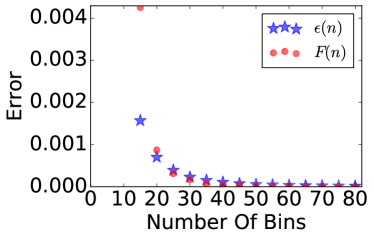
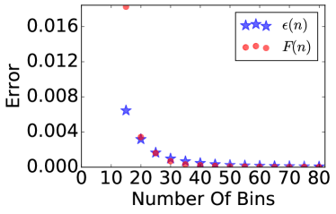
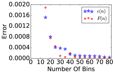
where 𝐱(t,n)𝐱𝑡𝑛\mathbf{x}(t,n), 𝐱(t,nj)𝐱𝑡𝑛superscript𝑗\mathbf{x}(t,n-j^{*}) are the vectors containing the fraction of nodes in each state at time t𝑡t, for the partitions Bn,Bnjsubscript𝐵𝑛subscript𝐵𝑛superscript𝑗B_{n},B_{n-j^{*}}, respectively. The step size j1superscript𝑗1{j}^{*}\geq 1 allows us to regulate how many steps (bins) are between two solutions we compare. In our implementation, we set j=5superscript𝑗5{j}^{*}=5, to obtain a smoother error function and to more easily detect the convergence of F(n)𝐹𝑛F(n). The basic idea of the heuristic is to increase n𝑛n and monitor the function F(n)𝐹𝑛F(n), stopping when we observe no noticable variation of its value. Although the partitions that we compute are refinements of each other for increasing n𝑛n, we cannot guarantee that ϵ(n)italic-ϵ𝑛\epsilon(n) and F(n)𝐹𝑛F(n) are always monotonically decreasing. However, ϵ(n)italic-ϵ𝑛\epsilon(n) eventually approaches zero and for all examples that we considered, small changes of F(n)𝐹𝑛F(n) for a number of steps indicated that with refinements of the corresponding partition Bnsubscript𝐵𝑛B_{n}, only very small improvements were possible in terms of ϵ(n)italic-ϵ𝑛\epsilon(n). In Fig. 3 (b) and (d) we see that F(n)𝐹𝑛F(n) is roughly proportional to ϵ(n)italic-ϵ𝑛\epsilon(n) and hence the difference F(n)F(nj)𝐹𝑛𝐹𝑛𝑗F(n)-F(n-j) can be used to identify the number n𝑛n beyond which ϵ(n)italic-ϵ𝑛\epsilon(n) decreases only very slowly. This proportionality between F(n)𝐹𝑛F(n) and ϵ(n)italic-ϵ𝑛\epsilon(n) was consistent for all models we have studied (see Fig. 3 (b) and (d)).

The above observation gives rise to the heuristic described in Algorithm 1 to decide the number of bins for the lumped equations based on a gradient descent approach. In the algorithm, j{1,,n1}𝑗1𝑛1j\in\{1,\ldots,n-1\} is a fixed (limited) lookahead used to approximate the gradient of F(n)𝐹𝑛F(n), and it is not necessarily equal to the step gap jsuperscript𝑗{j}^{*} used in the computation of F(n)𝐹𝑛F(n), even if in our implementation we used the same value, j=5𝑗5j=5, since smaller values (e.g. j=1𝑗1j=1) might not be as effective in indicating convergence. Apart from the model, the network degree distribution and the lookahead j𝑗j, Algorithm 1 takes as input a predefined threshold δ𝛿\delta and a parameter γnsubscript𝛾𝑛\gamma_{n} which is used for updating the number of bins for the next iteration. Note that increasing n𝑛n by a fixed number of bins in each step may lead to unnecessarily long running times. When n𝑛n is small, an increase of the number of bins often gives a large improvement, and hence F(n)𝐹𝑛-\nabla F(n) is large as well. In that case, a large increase of n𝑛n is adequate. In general, γnsubscript𝛾𝑛\gamma_{n} can be either fixed for every iteration, i.e., γn=γsubscript𝛾𝑛𝛾\gamma_{n}=\gamma, or it can adaptively be chosen by a backtracking line search method Wright and Nocedal (1999). In our implementation, we fixed δ=103𝛿superscript103\delta=10^{-3} and heuristically chose a fixed scaling constant γ=2103.𝛾2superscript103\gamma=2\cdot 10^{3}.

1:nj+j+1𝑛𝑗superscript𝑗1n\leftarrow j+j^{*}+1
2:Solve the lumped equations for all partitions necessary to compute F(n)𝐹𝑛F(n) and F(nj)𝐹𝑛𝑗F(n-j)
3:F(n)=F(n)F(nj)𝐹𝑛𝐹𝑛𝐹𝑛𝑗\nabla F(n)=F(n)-F(n-j)
4:if F(n)δ𝐹𝑛𝛿\nabla F(n)\leq\delta then
5:     return n.𝑛n.
6:else
7:     nn+max(1,𝖿𝗅𝗈𝗈𝗋(γnF(n)))𝑛𝑛1𝖿𝗅𝗈𝗈𝗋subscript𝛾𝑛𝐹𝑛n\leftarrow n+\max(1,\mathsf{floor}(-\gamma_{n}\nabla F(n))) and goto 2
Algorithm 1 (Heuristic to choose the number of bins)

IV.2 Results

We test our lumping approach for two well-studied models, namely the SIR model and a rumor spreading scenario, as well as for a third more complex system. For the simple SIR model, we tested our method for different degree distributions and investigated how the running time of the method increases when we vary the maximum degree kmaxsubscript𝑘maxk_{\mathrm{max}} of the network. For the rumor spreading model, we show that even with a small number of bins the method is able to capture contact processes with more than one contact rules. Finally, using the complex disease model, we verify that the method performs well even in cases of networks with many possible node states. For all models, we compare the dynamics and the running times of the original equations versus the lumped equations for a number of bins needed to get an error of at most 31033superscript1033\cdot 10^{-3}. Note that for each model we chose, whenever possible, parameter values s.t. the original DBMF equations differ significantly from the PA equations. In addition, we report the number of bins that was returned considering the stopping criterion of Algorithm 1. In well, we provide a user-friendly python tool, called LUMPY LUMPY Tool (2017), that takes a simple description of a contact process as input and a degree distribution. It automatically generates all kinds of equations, both the full ones and the lumped ones, using the binning heuristic discussed above.

SIR Model

The first model we examined is the SIR model, which consists of the following rules: a susceptible node S𝑆S that interacts with an infected node gets infected at rate θ1subscript𝜃1\theta_{1}; an infected node can recover at rate θ2subscript𝜃2\theta_{2}; and a recovered node can go back to the susceptible state at rate θ3subscript𝜃3\theta_{3}:

S+I𝑆𝐼\displaystyle S+I\; θ1subscript𝜃1\displaystyle\xrightarrow{\theta_{1}}   2I2𝐼\displaystyle\;\;2I
I𝐼\displaystyle I\; θ2subscript𝜃2\displaystyle\xrightarrow{\theta_{2}} R𝑅\displaystyle\;\;R
R𝑅\displaystyle R\; θ3subscript𝜃3\displaystyle\xrightarrow{\theta_{3}} S.𝑆\displaystyle\;\;S.

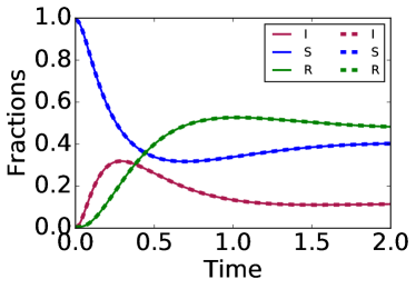
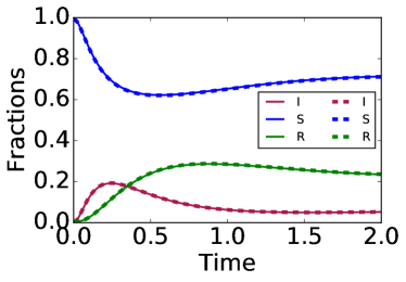
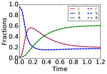
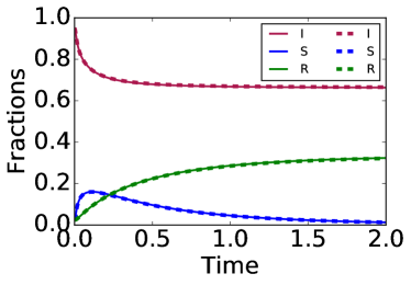
Here for all the experiments we set θ=(θ1,θ2,θ3)=(6,4,1)𝜃subscript𝜃1subscript𝜃2subscript𝜃3641\theta=(\theta_{1},\theta_{2},\theta_{3})=(6,4,1) and we assume the underlying network’s structure follows a power law distribution with kmax=103subscript𝑘maxsuperscript103k_{\mathrm{max}}=10^{3} and P(k)k2.4proportional-to𝑃𝑘superscript𝑘2.4P(k)\propto k^{-2.4}. In Fig. 3 we show the comparison between the dynamics of the aggregated DBMF equations using 20 bins and the original DBMF equations and in Fig. 3 we compare the aggregated PA equations for 21 bins and the original PA equations. We see that it in both cases is almost impossible to distinguish between the global measures derived from the aggregated ODEs and those obtained from the original system of equations. In Fig. 3 and 3 we plot the maximum error ϵ(n)italic-ϵ𝑛\epsilon(n) between the full and the lumped DBMF and PA equations, respectively, as a function of the number of bins n𝑛n as well as F(n)𝐹𝑛F(n), i.e., the maximum difference between the aggregated solutions for n𝑛n and nj𝑛𝑗n-j (j=5𝑗5j=5). Note that both errors quickly converge to zero as the number of bins increases.

In Fig. 4 and 4 we show the same plots for a network with uniform degree distribution P(k)=1/kmax,𝑃𝑘1subscript𝑘maxP(k)=1/k_{\mathrm{max}}, where kmax=500subscript𝑘max500k_{\mathrm{max}}=500, and the solution of the PA equations (aggregated vs. original ones). For the chosen network size the dynamics of DBMF equations completely agree with those of PA. Even though the uniform degree distribution is unrealistic for a typical contact network, we see that the lumped equations give very accurate results for a small number of bins. For an error ϵ(n)italic-ϵ𝑛\epsilon(n) of at most 31033superscript1033\cdot 10^{-3} we only need n=11𝑛11n=11 bins and 132132132 ODEs, in comparison to 500500500 degrees and 600060006000 ODEs of the full PA equations for this network. Note that the approximation works that accurately here, although due to the uniform assumption only the second part of the distance function in Eq. (23) (homogeneity of degrees) is considered in clustering.

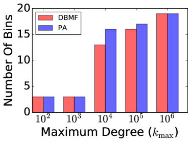
In Fig. 5 we plot the number of bins needed for the solution of the DBMF and PA equations for an approximation error of at most 31033superscript1033\cdot 10^{-3} in a power law network with varying kmax.subscript𝑘maxk_{\mathrm{max}}. The network size grows exponentially, while the number of bins needed grows only linearly. It is worth mentioning that in order to be sure that the dynamics of the network will change as kmaxsubscript𝑘maxk_{\mathrm{max}} increases, we have changed the parameter α𝛼\alpha of the power law in such a way that the coefficient of variation, i.e., σ/k𝜎delimited-⟨⟩𝑘\sigma/\!\left\langle k\right\rangle, of the distribution remains constant for different kmaxsubscript𝑘maxk_{\mathrm{max}} (see also Appendix, E).

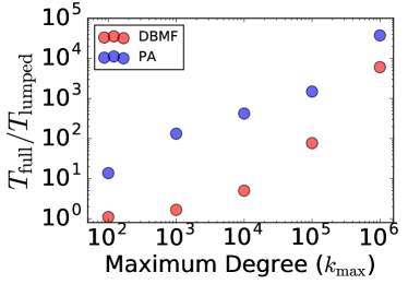
In Fig. 5 we plot the gain ratio Tfull/Tlumpedsubscript𝑇𝑓𝑢𝑙𝑙subscript𝑇𝑙𝑢𝑚𝑝𝑒𝑑T_{full}/T_{lumped} of the computation times for solving the aggregated equations instead of the full system. Generally the speedups are impressively high, and we see a significant increase of the ratio as the network size increases. In particular, for kmax=106subscript𝑘maxsuperscript106k_{\mathrm{max}}=10^{6} we need 5.25.25.2 days for solving the full equations, versus 121212 sec.​ for the lumped equations. The precise computation times of the needed lumped equations for varying kmaxsubscript𝑘maxk_{\mathrm{max}} are listed in Table 1, where the additional time needed for the hierarchical clustering is in the order of seconds up to network size kmax=104subscript𝑘maxsuperscript104k_{\mathrm{max}}=10^{4} and in the order of minutes up to kmax=106.subscript𝑘maxsuperscript106k_{\mathrm{max}}=10^{6}.

In Table 2 we include the number of bins returned by Algorithm 1, together with the corresponding error, for both DBMF and PA equations for varying kmaxsubscript𝑘maxk_{\mathrm{max}}. The number of bins returned by Algorithm 1 for δ=103𝛿superscript103\delta=10^{-3} yields very accurate approximations (error much-less-than\ll 31033superscript1033\cdot 10^{-3}), as the chosen stopping criterion of the heuristic is rather conservative. In any case, the speedups compared to a full solution of the equations are very similar to those in Fig. 5.

Table 1: SIR model: Running times (in seconds) of the full equations (Tfullsubscript𝑇fullT_{\mathrm{full}}) vs. running times of the lumped equations (Tlumpedsubscript𝑇lumpedT_{\mathrm{lumped}}) for all network sizes.
kmaxsubscript𝑘maxk_{\mathrm{max}} DBMF(Tfullsubscript𝑇fullT_{\mathrm{full}}) DBMF(Tlumpedsubscript𝑇lumpedT_{\mathrm{lumped}}) PA(Tfullsubscript𝑇fullT_{\mathrm{full}}) PA(Tlumpedsubscript𝑇lumpedT_{\mathrm{lumped}})
102superscript10210^{2} 3 2 1 0.07
103superscript10310^{3} 5 3 9 0.06
104superscript10410^{4} 10 2 126 0.32
105superscript10510^{5} 228 3 4428 3
106superscript10610^{6} 18177 3 449280 12
Table 2: SIR model: Number of bins returned by Alg. 1.
kmaxsubscript𝑘maxk_{\mathrm{max}} DBMF DBMF ϵitalic-ϵ\epsilon PA PA ϵitalic-ϵ\epsilon
102superscript10210^{2} 20 3.801073.80superscript1073.80\cdot 10^{-7} 20 2.701082.70superscript1082.70\cdot 10^{-8}
103superscript10310^{3} 20 6.051056.05superscript1056.05\cdot 10^{-5} 20 7.951067.95superscript1067.95\cdot 10^{-6}
104superscript10410^{4} 55 1.041041.04superscript1041.04\cdot 10^{-4} 56 1.801041.80superscript1041.80\cdot 10^{-4}
105superscript10510^{5} 37 4.471044.47superscript1044.47\cdot 10^{-4} 37 4.521044.52superscript1044.52\cdot 10^{-4}
106superscript10610^{6} 35 5.871045.87superscript1045.87\cdot 10^{-4} 35 6.181046.18superscript1046.18\cdot 10^{-4}
Refer to caption
Refer to caption
Refer to caption
Refer to caption
Figure 3: SIR model: Total fraction of infected (I)𝐼(I), susceptible (S)𝑆(S) and recovered (R)𝑅(R) nodes based on the original (solid lines) vs. the lumped (dashed lines) DBMF (a) and PA (c) equations for a power law network with kmax=103,P(k)k2.4formulae-sequencesubscript𝑘maxsuperscript103proportional-to𝑃𝑘superscript𝑘2.4k_{\mathrm{max}}=10^{3},P(k)\propto k^{-2.4}. The maximum error ϵ(n)italic-ϵ𝑛\epsilon(n) between the full and the aggregated equations w.r.t. the number of bins (\star) and the maximum difference F(n)𝐹𝑛F(n) between the aggregated solutions for two consecutive bin numbers (\circ) are shown for the DBMF (b) and the PA (d) lumping, respectively.
Refer to caption
Refer to caption
Figure 4: SIR model: (a): Total fraction of infected (I)𝐼(I), susceptible (S)𝑆(S) and recovered (R)𝑅(R) nodes based on the original (solid lines) vs. the lumped (dashed lines) PA equations for a uniform network with kmax=500,P(k)=1/kmax.formulae-sequencesubscript𝑘max500𝑃𝑘1subscript𝑘maxk_{\mathrm{max}}=500,P(k)=1/k_{\mathrm{max}}. (b): The maximum error ϵ(n)italic-ϵ𝑛\epsilon(n) between the full and the aggregated equations w.r.t.​​  the number of bins (\star) and the maximum difference F(n)𝐹𝑛F(n) between the aggregated solutions for two consecutive bin numbers (\circ) for the PA lumping.
Refer to caption
Refer to caption
Figure 5: SIR model: The number of bins needed for an approximation error of at most 31033superscript1033\cdot 10^{-3} for the solution of the DBMF and PA equations and for varying kmaxsubscript𝑘maxk_{\mathrm{max}} (a), and the gain ratio of the computation times Tfull/Tlumpedsubscript𝑇fullsubscript𝑇lumpedT_{\mathrm{full}}/T_{\mathrm{lumped}} of lumped DBMF and PA equations for different kmaxsubscript𝑘maxk_{\mathrm{max}} (b).

Rumor Spreading Model

As a second model, we consider a rumor spreading model Barrat et al. (2008) that includes three different types of individuals: ignorants (I), spreaders (S), and stiflers (R). An ignorant that is in contact with a spreader becomes a spreader at rate λ.𝜆\lambda. A spreader becomes a stifler when the spreader is in contact either with a spreader or a stifler; in both cases the corresponding transition rate is α𝛼\alpha:

S+I𝑆𝐼\displaystyle S+I\; 𝜆𝜆\displaystyle\xrightarrow{\lambda}   2S2𝑆\displaystyle\;\;2S
S+R𝑆𝑅\displaystyle S+R\; 𝛼𝛼\displaystyle\xrightarrow{\alpha}   2R2𝑅\displaystyle\;\;2R
2S2𝑆\displaystyle 2S\; 𝛼𝛼\displaystyle\xrightarrow{\alpha} S+R.𝑆𝑅\displaystyle\;\;S+R.

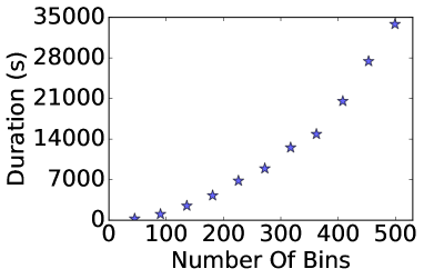
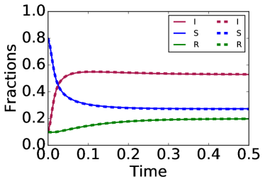
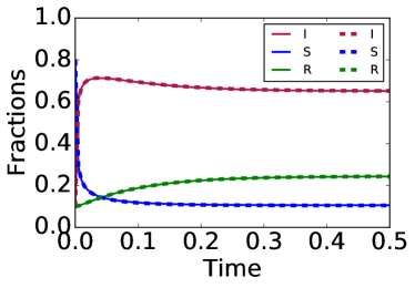
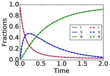
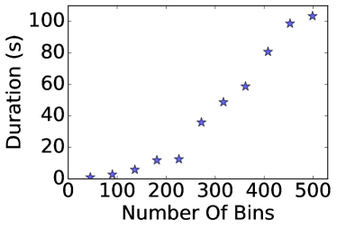
Here, we set λ=6.0𝜆6.0\lambda=6.0 and α=0.7𝛼0.7\alpha=0.7 and, for the network’s degree distribution, we consider a truncated power law P(k)k2.2proportional-to𝑃𝑘superscript𝑘2.2P(k)\propto k^{-2.2} with kmax=500.subscript𝑘max500k_{\mathrm{max}}=500. In Fig. 6 we show the dynamics of the full DBMF ODEs compared to the DBMF lumped equations and in Fig. 6 the corresponding comparison for the PA equations. We note that DBMF here gives a poor approximation, which is qualitatively different from the PA solution. Even though there is a great difference between the solutions of the two systems of equations, the lumped equations approximate very accurately the original equations for both cases. For this model, we needed only 13 bins and 39 ODEs for the DBMF case and 27 bins and 324 ODEs for the PA in order to get a maximum error of 31033superscript1033\cdot 10^{-3}. The heuristic in Alg. 1 with δ=103𝛿superscript103\delta=10^{-3} returned 43 bins with an error of 104superscript10410^{-4} for the first and 60 bins with an error of 21042superscript1042\cdot 10^{-4} for the second case. The computation times for solving the lumped equations of DBMF and PA for every possible number of bins are shown in Fig. 6 (b) and (d). Again, we see huge computational gains when solving the lumped equations instead, especially in the case of PA.
Refer to caption
Refer to caption
Refer to caption
Refer to caption
Figure 6: Rumor spreading model: Total fraction of ignorant (I)𝐼(I), spreaders (S)𝑆(S) and stiflers (R)𝑅(R) in a power law network with kmax=500subscript𝑘max500k_{\mathrm{max}}=500 for the original DBMF (a) and PA (c) equations (solid lines) and solution of the corresponding lumped equations (dashed lines). ::\star: The running time of the aggregated equations w.r.t. the number of bins used for DBMF (b) and PA (d).

SIIIR Model

Recent infection models describe the infection process in more detail by considering multiple infection phases Miller and Volz (2013). In HIV, for instance, the early phase is well known to be significantly more infectious than a longer-lasting chronic phase Pilcher et al. (2004); Eames and Keeling (2002). In order to capture such behavior, here we incorporate the phases as different states of the individuals, i.e., I,II,III,𝐼𝐼𝐼𝐼𝐼𝐼I,II,III, with different transmission rates:

S+I𝑆𝐼\displaystyle S+I\; θ1subscript𝜃1\displaystyle\xrightarrow{\theta_{1}}   2I2𝐼\displaystyle\;\;2I\hskip 8.0pt II𝐼𝐼\displaystyle II\; θ5subscript𝜃5\displaystyle\xrightarrow{\theta_{5}} III𝐼𝐼𝐼\displaystyle\;\;III\hskip 8.0pt
S+II𝑆𝐼𝐼\displaystyle S+II\; θ2subscript𝜃2\displaystyle\xrightarrow{\theta_{2}} I+II𝐼𝐼𝐼\displaystyle\;\;I+II III𝐼𝐼𝐼\displaystyle III\; θ6subscript𝜃6\displaystyle\xrightarrow{\theta_{6}} R𝑅\displaystyle\;\;R
S+III𝑆𝐼𝐼𝐼\displaystyle S+III\; θ3subscript𝜃3\displaystyle\xrightarrow{\theta_{3}} I+III𝐼𝐼𝐼𝐼\displaystyle\;\;I+III\hskip 8.0pt R𝑅\displaystyle R\; θ7subscript𝜃7\displaystyle\xrightarrow{\theta_{7}} S𝑆\displaystyle\;\;S
I𝐼\displaystyle I\; θ4subscript𝜃4\displaystyle\xrightarrow{\theta_{4}} II𝐼𝐼\displaystyle\;\;II

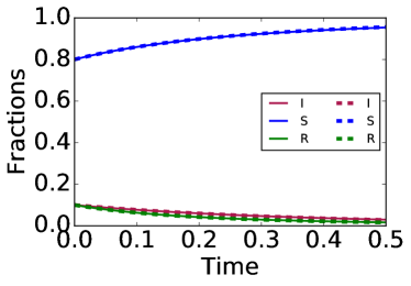
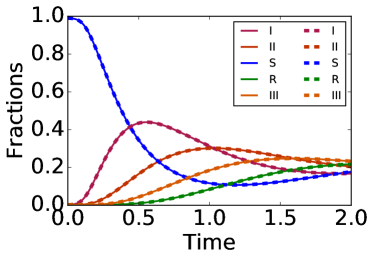
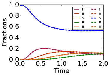
We fix θ=(θ1,,θ7)=(5,1.5,1,2,2,2,2)𝜃subscript𝜃1subscript𝜃751.512222\theta=(\theta_{1},\ldots,\theta_{7})=(5,1.5,1,2,2,2,2) and we test our lumped equations with the original DBMF and PA solutions taken for the scale-free network (P(k)k2.5,kmax=100)formulae-sequenceproportional-to𝑃𝑘superscript𝑘2.5subscript𝑘max100(P(k)\propto k^{-2.5},k_{\mathrm{max}}=100) of sexual partners over a time period of one year Liljeros et al. (2001). Despite the large number of possible node states, the dynamics of the total fractions of all states is captured very accurately (error of less than 31033superscript1033\cdot 10^{-3}) by the lumped equations with 20 bins in both DBMF (Fig. 7) and PA (Fig. 7). For this system, Algorithm 1 returned 39 bins for DBMF and 46 bins for PA with an error of 4.71054.7superscript1054.7\cdot 10^{-5} and 51055superscript1055\cdot 10^{-5}, respectively, when δ=103𝛿superscript103\delta=10^{-3} was chosen. Last, it is worth mentioning that we also tested the robustness of our method regarding the choice of the initial fractions. In Gleeson (2011) and Gleeson (2013) the author uses for each state s𝑠s a constant initial fraction for all xs,ksubscript𝑥𝑠𝑘x_{s,k} for every k𝑘k, which is equal to the initial total fraction of xs.subscript𝑥𝑠x_{s}. Here, we considered in addition completely random initial fractions for each xs,ksubscript𝑥𝑠𝑘x_{s,k} for all states s𝑠s, and this initialization returned an even smaller error function in the beginning (see also Appendix, F), mainly because we avoid the extreme values that might be present in our initialization, such as the total fraction of susceptible nodes, which is here close to one. Hence, we conclude that the method is robust against different initial conditions.
Refer to caption
Refer to caption
Figure 7: SIIIR model: Total fraction of infected (I),(II),(III)𝐼𝐼𝐼𝐼𝐼𝐼(I),(II),(III) nodes of phase I,II,III𝐼𝐼𝐼𝐼𝐼𝐼I,II,III, respectively, susceptible (S)𝑆(S) and recovered (R)𝑅(R) nodes in a power law network with kmax=100,P(k)k2.5formulae-sequencesubscript𝑘max100proportional-to𝑃𝑘superscript𝑘2.5k_{\mathrm{max}}=100,P(k)\propto k^{-2.5}. The solid lines show the solution of the original DBMF (a) and PA (b) equations, and the dashed lines the solution of the corresponding lumped DBMF (a) and PA (b) equations.

V Conclusion

Studying complex dynamic processes happening on networks is a daunting computational task when relying on simulation. To ameliorate this problem, several forms of approximations have been considered, all trying to take the topology of the network into account to some extent: degree-based mean-field Pastor-Satorras and Vespignani (2001), AME, and pair approximation Gleeson (2013). AME and PA equations, in particular, seem to capture with precision the dynamics of a large variety of network topologies, but in Gleeson (2013) they are typically restricted to the binary case, i.e., to processes with only two local states. Here, we consider the AME and the subsequent derivation of the PA in the general case of contact processes of n𝑛n states. The total number of equations for both DBMF and PA is directly dependent on the maximum degree, |S|kmax𝑆subscript𝑘max|S|k_{\mathrm{max}} and |S|2kmaxsuperscript𝑆2subscript𝑘max|S|^{2}k_{\mathrm{max}}, respectively, and hence the total computation time even for these approximate methods can be demanding for large networks with many states.

In this paper, we argue that although the network structure is proven to be essential for its dynamics, we do not need a full resolution to get precise results for the time evolution of the total fractions. For instance, it is expected that the degrees belonging to the tail of a power law should not significantly change the precision of the equations if clustered together. Motivated by this insight, we investigated whether it is possible to capture the dynamics of DBMF and PA equations by solving a smaller set of equations. Taking advantage of the degree distribution characteristics, and additionally exploiting a notion of homogeneity of the differences between separate degrees, we provide a mechanism according to which we can effectively reduce the resolution of network degrees, clustering them into a small number of bins and constructing a small set of aggregated differential equations.

The results in terms of computational gain are particularly impressive: we manage to approximate collective network statistics, namely the total fractions of nodes in each state, produced by DBMF and PA equations by solving a significantly smaller number of differential equations and gaining a computational speedup of several orders of magnitude. We are able to reproduce these results for a number of different network degree distributions and a number of different models.

Furthermore, the procedure to construct the reduced set of equations is fully automatic, and it is implemented as an open-source Python tool LUMPY Tool (2017). The tool takes a compact description of the model as input and returns Python files containing the lumped and the full DBMF and PA equations as output. This makes validation of the results and experimentation with other models a very easy task.

The natural direction in which to extend this work is to provide a similar approach to aggregate the AME equations. A direct strategy would be to use the same binning as for PA equations and lump AME only over different degrees k𝑘k. For each of the formed bins, we would then need to solve |S||𝕄kmaxb|𝑆subscript𝕄subscriptsuperscript𝑘𝑏max|S||\mathbb{M}_{k^{b}_{\mathrm{max}}}| equations. This is guaranteed to give at least as good results as the lumped PA equations. The quality, however, may depend on whether the solution of the original PA equations is close to the solution of the AME. However, getting a simultaneous aggregation over degrees kK𝑘𝐾k\in K and neighbors 𝕞𝕄k𝕞subscript𝕄𝑘\mathbb{m}\in\mathbb{M}_{k} which is close to the solution of full AME equations could give a tremendous computational boost and make AME tractable regardless of the network size. Finally, a modification of the presented lumping method could successfully be applied to adaptive networks, where the degree distribution changes smoothly over time. In this case, we expect that “on-the-fly” and local rearrangements of the clusters could be sufficient to capture well the topology changes of such networks.

Acknowledgements.
We would like to thank Mayank Goyal for an early implementation of the binning approach on the binary state case dynamics as part of his master’s thesis.

Appendix A State distribution of the neighborhood in uncorrelated networks

In this section, we prove Eq. (3) for uncorrelated networks, i.e., pk[s]=p[s]=1/kkKP(k)kxs,ksubscript𝑝𝑘delimited-[]superscript𝑠𝑝delimited-[]superscript𝑠1delimited-⟨⟩𝑘subscriptsuperscript𝑘𝐾𝑃superscript𝑘superscript𝑘subscript𝑥superscript𝑠superscript𝑘p_{k}[s^{\prime}]=p[s^{\prime}]=1/{\left\langle k\right\rangle}\sum_{k^{\prime}\in K}{P(k^{\prime})k^{\prime}x_{s^{\prime},k^{\prime}}}.

We consider first the probability qk(k)subscript𝑞𝑘superscript𝑘q_{k}(k^{\prime}) that, given a node of degree k𝑘k, a randomly chosen direct neighbor of it has degree ksuperscript𝑘k^{\prime}. Since in an uncorrelated network the above probability is independent of k𝑘k, it is the same as the probability q(k)𝑞superscript𝑘q(k^{\prime}) of choosing a random edge that connects to a node of degree ksuperscript𝑘k^{\prime}. Hence:

qk(k)=q(k)subscript𝑞𝑘superscript𝑘𝑞superscript𝑘\displaystyle q_{k}(k^{\prime})=q(k^{\prime})
=\displaystyle= #(edgesconnectedtoknode)#(edgesconnectedtoarbitrarynode)#edgesconnectedtosuperscriptknode#edgesconnectedtoarbitrarynode\displaystyle\frac{\#(\mathrm{edges\;connected\;to\;k^{\prime}\;node})}{\#(\mathrm{edges\;connected\;to\;arbitrary\;node})}
=\displaystyle= kNk2|E|=kNk/N2|E|/N=kP(k)k,superscript𝑘subscript𝑁superscript𝑘2𝐸superscript𝑘subscript𝑁superscript𝑘𝑁2𝐸𝑁superscript𝑘𝑃superscript𝑘delimited-⟨⟩𝑘\displaystyle\frac{k^{\prime}N_{k^{\prime}}}{2|E|}=\frac{k^{\prime}N_{k^{\prime}}/N}{2|E|/N}=\frac{k^{\prime}P(k^{\prime})}{\left\langle k\right\rangle},

where Nksubscript𝑁superscript𝑘N_{k^{\prime}} is the number of nodes of degree ksuperscript𝑘k^{\prime} and |E|𝐸|E| is the total number of edges. Please note here the subtle but important difference between q(k)𝑞superscript𝑘q(k^{\prime}), which is the probability of picking a ksuperscript𝑘k^{\prime} node after randomly choosing a network edge, and P(k)𝑃superscript𝑘P(k^{\prime}), which is the probability of a random node being of degree ksuperscript𝑘k^{\prime}. Thus the probability that a random neighbor of a node of degree k𝑘k in an uncorrelated network is in state ssuperscript𝑠s^{\prime} is independent of k𝑘k, and given by:

pk[s]=p[s]=kKxs,kq(k)subscript𝑝𝑘delimited-[]superscript𝑠𝑝delimited-[]superscript𝑠subscriptsuperscript𝑘𝐾subscript𝑥superscript𝑠superscript𝑘𝑞superscript𝑘\displaystyle p_{k}[s^{\prime}]=p[s^{\prime}]=\sum_{k^{\prime}\in K}x_{s^{\prime},k^{\prime}}q(k^{\prime})
=\displaystyle= kKxs,kkP(k)k.subscriptsuperscript𝑘𝐾subscript𝑥superscript𝑠superscript𝑘superscript𝑘𝑃superscript𝑘delimited-⟨⟩𝑘\displaystyle\sum_{k^{\prime}\in K}x_{s^{\prime},k^{\prime}}\frac{k^{\prime}P(k^{\prime})}{\left\langle k\right\rangle}.

Appendix B Number of AME equations

Without considering the redundant equations, the number of equations of the general AME case with |S|𝑆|S| states is (kmax+|S||S|1)(kmax+1).binomialsubscript𝑘max𝑆𝑆1subscript𝑘max1\binom{k_{\mathrm{max}}+|S|}{|S|-1}(k_{\mathrm{max}}+1).

Proof:

|S|k=0kmax(k+|S|1|S|1)=|S|(kmax+|S||S|)𝑆superscriptsubscript𝑘0subscript𝑘maxbinomial𝑘𝑆1𝑆1𝑆binomialsubscript𝑘max𝑆𝑆\displaystyle|S|\sum_{k=0}^{k_{\mathrm{max}}}\binom{k+|S|-1}{|S|-1}=|S|\binom{k_{\mathrm{max}}+|S|}{|S|} (25)
=\displaystyle= |S|(kmax+|S|)!|S|!kmax!=(kmax+|S|)!(|S|1)!(kmax+1)!(kmax+1)𝑆subscript𝑘max𝑆𝑆subscript𝑘maxsubscript𝑘max𝑆𝑆1subscript𝑘max1subscript𝑘max1\displaystyle|S|\frac{(k_{\mathrm{max}}+|S|)!}{|S|!\;k_{\mathrm{max}}!}=\frac{(k_{\mathrm{max}}+|S|)!}{(|S|-1)!\;(k_{\mathrm{max}}+1)!}(k_{\mathrm{max}}+1)
=\displaystyle= (kmax+|S||S|1)(kmax+1).binomialsubscript𝑘max𝑆𝑆1subscript𝑘max1\displaystyle\binom{k_{\mathrm{max}}+|S|}{|S|-1}(k_{\mathrm{max}}+1).

The first equality is the rising sum of binomial coefficients and the rest is simple calculus.

Appendix C From AME to PA

Proof: We consider the general case of the AME equation in (4) for |S|𝑆|S| states and NIsubscript𝑁𝐼N_{I} + NCsubscript𝑁𝐶N_{C} rules. Assuming that the number of links of an (s,k)𝑠𝑘(s,k) node to all other states is multinomially distributed, we get two equations: The first equation describes the fraction of (s,k)𝑠𝑘(s,k) nodes and the second equation the probability ps,k[sn]subscript𝑝𝑠𝑘delimited-[]subscript𝑠𝑛p_{s,k}[s_{n}] that a random neighbor of (s,k)𝑠𝑘(s,k) is in state snsubscript𝑠𝑛s_{n}.

\circ In order to derive an expression for the fraction of (s,k)𝑠𝑘(s,k) nodes, we sum up both parts of (4) over all possible vectors 𝕞𝕄k,𝕞subscript𝕄𝑘\mathbb{m}\in\mathbb{M}_{k}, where 𝕄ksubscript𝕄𝑘\mathbb{M}_{k} is the support of the multinomial distribution, and we apply the multinomial assumption to all terms. This yields

t𝕞𝕄kxs,k,𝕞=𝑡subscript𝕞subscript𝕄𝑘subscript𝑥𝑠𝑘𝕞absent\displaystyle\frac{\partial}{\partial t}\sum_{\mathbb{m}\in\mathbb{M}_{k}}x_{s,k,\mathbb{m}}=
RI,iRIs+λi𝕞𝕄kxri,k,𝕞RI,iRIsλi𝕞𝕄kxs,k,𝕞subscriptsubscript𝑅𝐼𝑖subscriptsuperscript𝑅superscript𝑠𝐼subscript𝜆𝑖subscript𝕞subscript𝕄𝑘subscript𝑥subscript𝑟𝑖𝑘𝕞subscriptsubscript𝑅𝐼𝑖subscriptsuperscript𝑅superscript𝑠𝐼subscript𝜆𝑖subscript𝕞subscript𝕄𝑘subscript𝑥𝑠𝑘𝕞\displaystyle\sum_{R_{I,i}\in R^{s^{+}}_{I}}\lambda_{i}\sum_{\mathbb{m}\in\mathbb{M}_{k}}x_{r_{i},k,\mathbb{m}}-\sum_{R_{I,i}\in R^{s^{-}}_{I}}\lambda_{i}\sum_{\mathbb{m}\in\mathbb{M}_{k}}x_{s,k,\mathbb{m}}
+\displaystyle+ RC,jRCs+λj𝕞𝕄kxrj1,k,𝕞𝕞[rj2]subscriptsubscript𝑅𝐶𝑗subscriptsuperscript𝑅superscript𝑠𝐶subscript𝜆𝑗subscript𝕞subscript𝕄𝑘subscript𝑥subscript𝑟subscript𝑗1𝑘𝕞𝕞delimited-[]subscript𝑟subscript𝑗2\displaystyle\sum_{R_{C,j}\in R^{s^{+}}_{C}}\lambda_{j}\sum_{\mathbb{m}\in\mathbb{M}_{k}}x_{r_{j_{1}},k,\mathbb{m}}\mathbb{m}[r_{j_{2}}]
\displaystyle- RC,jRCsλj𝕞𝕄kxs,k,𝕞𝕞[rj2]subscriptsubscript𝑅𝐶𝑗subscriptsuperscript𝑅superscript𝑠𝐶subscript𝜆𝑗subscript𝕞subscript𝕄𝑘subscript𝑥𝑠𝑘𝕞𝕞delimited-[]subscript𝑟subscript𝑗2\displaystyle\sum_{R_{C,j}\in R^{s^{-}}_{C}}\lambda_{j}\sum_{\mathbb{m}\in\mathbb{M}_{k}}x_{s,k,\mathbb{m}}\mathbb{m}[r_{j_{2}}]
+\displaystyle+ (s,s′′)S2ss′′βssss′′𝕞𝕄k𝕞[s′′]1,𝕞[s]<kxs,k,𝕞{s+,s′′}𝕞{s+,s′′}[s]subscriptsuperscript𝑠superscript𝑠′′superscript𝑆2superscript𝑠superscript𝑠′′superscript𝛽𝑠superscript𝑠𝑠superscript𝑠′′subscript𝕞subscript𝕄𝑘formulae-sequence𝕞delimited-[]superscript𝑠′′1𝕞delimited-[]superscript𝑠𝑘subscript𝑥𝑠𝑘superscript𝕞superscript𝑠superscript𝑠′′superscript𝕞superscript𝑠superscript𝑠′′delimited-[]superscript𝑠\displaystyle\sum_{\begin{subarray}{c}(s^{\prime},s^{\prime\prime})\in S^{2}\\ s^{\prime}\neq s^{\prime\prime}\end{subarray}}\beta^{ss^{\prime}\rightarrow ss^{\prime\prime}}\!\!\!\!\!\!\sum_{\begin{subarray}{c}\mathbb{m}\in\mathbb{M}_{k}\\ \mathbb{m}[s^{\prime\prime}]\geq 1,\mathbb{m}[s^{\prime}]<k\end{subarray}}\!\!\!\!\!x_{s,k,\mathbb{m}^{\{s^{\prime+},s^{\prime\prime-}\}}}\mathbb{m}^{\{s^{\prime+},s^{\prime\prime-}\}}[s^{\prime}]
\displaystyle- (s,s′′)S2ss′′βssss′′𝕞𝕄kxs,k,𝕞𝕞[s],sS,kK,formulae-sequencesubscriptsuperscript𝑠superscript𝑠′′superscript𝑆2superscript𝑠superscript𝑠′′superscript𝛽𝑠superscript𝑠𝑠superscript𝑠′′subscript𝕞subscript𝕄𝑘subscript𝑥𝑠𝑘𝕞𝕞delimited-[]superscript𝑠for-all𝑠𝑆for-all𝑘𝐾\displaystyle\sum_{\begin{subarray}{c}(s^{\prime},s^{\prime\prime})\in S^{2}\\ s^{\prime}\neq s^{\prime\prime}\end{subarray}}\beta^{ss^{\prime}\rightarrow ss^{\prime\prime}}\!\!\!\!\sum_{\mathbb{m}\in\mathbb{M}_{k}}x_{s,k,\mathbb{m}}\mathbb{m}[s^{\prime}],\hskip 14.22636pt\forall s\in S,\;\forall k\in K,

which after simplification becomes

txs,k=RI,iRIs+λixri,kRI,iRIsλixs,k𝑡subscript𝑥𝑠𝑘subscriptsubscript𝑅𝐼𝑖subscriptsuperscript𝑅superscript𝑠𝐼subscript𝜆𝑖subscript𝑥subscript𝑟𝑖𝑘subscriptsubscript𝑅𝐼𝑖subscriptsuperscript𝑅superscript𝑠𝐼subscript𝜆𝑖subscript𝑥𝑠𝑘\displaystyle\frac{\partial}{\partial t}x_{s,k}=\sum_{R_{I,i}\in R^{s^{+}}_{I}}\lambda_{i}x_{r_{i},k}-\sum_{R_{I,i}\in R^{s^{-}}_{I}}\lambda_{i}x_{s,k}
+\displaystyle+ RC,jRCs+λjxrj1,kμrj1,k(rj2)RC,jRCsλjxs,kμs,k(rj2).subscriptsubscript𝑅𝐶𝑗subscriptsuperscript𝑅superscript𝑠𝐶subscript𝜆𝑗subscript𝑥subscript𝑟subscript𝑗1𝑘subscript𝜇subscript𝑟subscript𝑗1𝑘subscript𝑟subscript𝑗2subscriptsubscript𝑅𝐶𝑗subscriptsuperscript𝑅superscript𝑠𝐶subscript𝜆𝑗subscript𝑥𝑠𝑘subscript𝜇𝑠𝑘subscript𝑟subscript𝑗2\displaystyle\sum_{R_{C,j}\in R^{s^{+}}_{C}}\lambda_{j}x_{r_{j_{1}},k}{\mu}_{r_{j_{1}},k}(r_{j_{2}})\quad-\sum_{R_{C,j}\in R^{s^{-}}_{C}}\lambda_{j}x_{s,k}{\mu}_{s,k}(r_{j_{2}}).

Here, μs,k(si)subscript𝜇𝑠𝑘subscript𝑠𝑖{\mu}_{s,k}(s_{i}) denotes the average of the i𝑖i-th entry over all 𝕞𝕞\mathbb{m} vectors of (s,k)𝑠𝑘(s,k) nodes. Applying the multinomial assumption, it holds that μs,k(si)=𝕞𝕄kf(𝕞,ps,k)𝕞[si]=kps,k[si],subscript𝜇𝑠𝑘subscript𝑠𝑖subscript𝕞subscript𝕄𝑘𝑓𝕞subscript𝑝𝑠𝑘𝕞delimited-[]subscript𝑠𝑖𝑘subscript𝑝𝑠𝑘delimited-[]subscript𝑠𝑖{\mu}_{s,k}(s_{i})=\sum_{\mathbb{m}\in\mathbb{M}_{k}}f(\mathbb{m},p_{s,k})\mathbb{m}[s_{i}]=kp_{s,k}[s_{i}], where f(𝕞,ps,k)𝑓𝕞subscript𝑝𝑠𝑘f(\mathbb{m},p_{s,k}) is the probability of picking a neighbor vector 𝕞𝕞\mathbb{m} from a multinomial distribution with a vector of success probabilities equal to ps,k.subscript𝑝𝑠𝑘p_{s,k}.

Note that the last two terms in (C) cancel out because

𝕞𝕄k𝕞[s]<k𝕞[s′′]1xs,k,𝕞{s+,s′′}(𝕞[s]+1)=𝕞𝕄k𝕞[s]1𝕞[s′′]<kxs,k,𝕞𝕞[s]=subscript𝕞subscript𝕄𝑘𝕞delimited-[]superscript𝑠𝑘𝕞delimited-[]superscript𝑠′′1subscript𝑥𝑠𝑘superscript𝕞superscript𝑠superscript𝑠′′𝕞delimited-[]superscript𝑠1subscript𝕞subscript𝕄𝑘𝕞delimited-[]superscript𝑠1𝕞delimited-[]superscript𝑠′′𝑘subscript𝑥𝑠𝑘𝕞𝕞delimited-[]superscript𝑠absent\displaystyle\sum_{\begin{subarray}{c}\mathbb{m}\in\mathbb{M}_{k}\\ \mathbb{m}[s^{\prime}]<k\\ \mathbb{m}[s^{\prime\prime}]\geq 1\end{subarray}}\;x_{s,k,\mathbb{m}^{\{s^{\prime+},s^{\prime\prime-}\}}}(\mathbb{m}[s^{\prime}]+1)=\sum_{\begin{subarray}{c}\mathbb{m}\in\mathbb{M}_{k}\\ \mathbb{m}[s^{\prime}]\geq 1\\ \mathbb{m}[s^{\prime\prime}]<k\end{subarray}}\;x_{s,k,\mathbb{m}}\mathbb{m}[s^{\prime}]=
𝕞𝕄kxs,k,𝕞𝕞[s],subscript𝕞subscript𝕄𝑘subscript𝑥𝑠𝑘𝕞𝕞delimited-[]superscript𝑠\displaystyle\sum_{\begin{subarray}{c}\mathbb{m}\in\mathbb{M}_{k}\end{subarray}}\;x_{s,k,\mathbb{m}}\mathbb{m}[s^{\prime}], (28)

where the last equality follows from the fact that when 𝕞[s′′]=k𝕞delimited-[]superscript𝑠′′𝑘\mathbb{m}[s^{\prime\prime}]=k then 𝕞[s]=0𝕞delimited-[]superscript𝑠0\mathbb{m}[s^{\prime}]=0.

\circ To derive an equation for ps,k[sn]subscript𝑝𝑠𝑘delimited-[]subscript𝑠𝑛p_{s,k}[s_{n}], we first consider the change over time of the number of edges between a node in state s𝑠s and snsubscript𝑠𝑛s_{n}. From the multinomial assumption, we have that

t𝕞𝕄kxs,k,𝕞𝕞[sn]𝑡subscript𝕞subscript𝕄𝑘subscript𝑥𝑠𝑘𝕞𝕞delimited-[]subscript𝑠𝑛\displaystyle\frac{\partial}{\partial t}\sum_{\mathbb{m}\in\mathbb{M}_{k}}x_{s,k,\mathbb{m}}\mathbb{m}[s_{n}] =\displaystyle= t(xs,k𝕞𝕄kf(𝕞,ps,k)𝕞[sn])𝑡subscript𝑥𝑠𝑘subscript𝕞subscript𝕄𝑘𝑓𝕞subscript𝑝𝑠𝑘𝕞delimited-[]subscript𝑠𝑛\displaystyle\frac{\partial}{\partial t}\bigg{(}x_{s,k}\sum_{\mathbb{m}\in\mathbb{M}_{k}}f(\mathbb{m},p_{s,k})\mathbb{m}[s_{n}]\bigg{)} (29)
=\displaystyle= t(xs,kkps,k[sn]),𝑡subscript𝑥𝑠𝑘𝑘subscript𝑝𝑠𝑘delimited-[]subscript𝑠𝑛\displaystyle\frac{\partial}{\partial t}(x_{s,k}kp_{s,k}[s_{n}]),

where f(𝕞,ps,k)𝑓𝕞subscript𝑝𝑠𝑘f(\mathbb{m},p_{s,k}) is the probability of picking a neighbor vector 𝕞𝕞\mathbb{m} from a multinomial distribution with a vector of success probabilities equal to ps,k.subscript𝑝𝑠𝑘p_{s,k}. Using similar arguments, we can now derive an expression for (29) by summation of (4) after multiplication of 𝕞[sn]𝕞delimited-[]subscript𝑠𝑛\mathbb{m}[s_{n}].

t(xs,kkps,k[sn])=𝑡subscript𝑥𝑠𝑘𝑘subscript𝑝𝑠𝑘delimited-[]subscript𝑠𝑛absent\displaystyle\qquad\frac{\partial}{\partial t}(x_{s,k}kp_{s,k}[s_{n}])=
RI,iRIs+λi𝕞𝕄kxri,kf(𝕞,pri,k)𝕞[sn]subscriptsubscript𝑅𝐼𝑖subscriptsuperscript𝑅superscript𝑠𝐼subscript𝜆𝑖subscript𝕞subscript𝕄𝑘subscript𝑥subscript𝑟𝑖𝑘𝑓𝕞subscript𝑝subscript𝑟𝑖𝑘𝕞delimited-[]subscript𝑠𝑛\displaystyle\sum_{R_{I,i}\in R^{s^{+}}_{I}}\lambda_{i}\sum_{\mathbb{m}\in\mathbb{M}_{k}}x_{r_{i},k}f(\mathbb{m},p_{r_{i},k})\mathbb{m}[s_{n}]
RI,iRIsλi𝕞𝕄kxs,kf(𝕞,ps,k)𝕞[sn]subscriptsubscript𝑅𝐼𝑖subscriptsuperscript𝑅superscript𝑠𝐼subscript𝜆𝑖subscript𝕞subscript𝕄𝑘subscript𝑥𝑠𝑘𝑓𝕞subscript𝑝𝑠𝑘𝕞delimited-[]subscript𝑠𝑛\displaystyle-\sum_{R_{I,i}\in R^{s^{-}}_{I}}\lambda_{i}\sum_{\mathbb{m}\in\mathbb{M}_{k}}x_{s,k}f(\mathbb{m},p_{s,k})\mathbb{m}[s_{n}]
+RC,jRCs+λj𝕞𝕄kxrj1,kf(𝕞,prj1,k)𝕞[sn]𝕞[rj2]subscriptsubscript𝑅𝐶𝑗subscriptsuperscript𝑅superscript𝑠𝐶subscript𝜆𝑗subscript𝕞subscript𝕄𝑘subscript𝑥subscript𝑟subscript𝑗1𝑘𝑓𝕞subscript𝑝subscript𝑟subscript𝑗1𝑘𝕞delimited-[]subscript𝑠𝑛𝕞delimited-[]subscript𝑟subscript𝑗2\displaystyle+\sum_{R_{C,j}\in R^{s^{+}}_{C}}\lambda_{j}\sum_{\mathbb{m}\in\mathbb{M}_{k}}x_{r_{j_{1}},k}f(\mathbb{m},p_{{r_{j_{1}},k}})\mathbb{m}[s_{n}]\mathbb{m}[r_{j_{2}}]
RC,jRCsλj𝕞𝕄kxs,kf(𝕞,ps,k)𝕞[sn]𝕞[rj2]subscriptsubscript𝑅𝐶𝑗subscriptsuperscript𝑅superscript𝑠𝐶subscript𝜆𝑗subscript𝕞subscript𝕄𝑘subscript𝑥𝑠𝑘𝑓𝕞subscript𝑝𝑠𝑘𝕞delimited-[]subscript𝑠𝑛𝕞delimited-[]subscript𝑟subscript𝑗2\displaystyle-\sum_{R_{C,j}\in R^{s^{-}}_{C}}\lambda_{j}\sum_{\mathbb{m}\in\mathbb{M}_{k}}x_{s,k}f(\mathbb{m},p_{s,k})\mathbb{m}[s_{n}]\mathbb{m}[r_{j_{2}}]
+(s,s′′)S2ss′′βssss′′(𝕞𝕄k𝕞[s]<k𝕞[s′′]1xs,k,𝕞{s+,s′′}𝕞{s+,s′′}[s]𝕞[sn](1)\displaystyle+\!\!\!\!\!\sum_{\begin{subarray}{c}(s^{\prime},s^{\prime\prime})\in S^{2}\\ s^{\prime}\neq s^{\prime\prime}\end{subarray}}\!\!\!\!\!\beta^{ss^{\prime}\rightarrow ss^{\prime\prime}}\Bigg{(}\!\!\underbrace{\sum_{\begin{subarray}{c}\mathbb{m}\in\mathbb{M}_{k}\\ \mathbb{m}[s^{\prime}]<k\\ \mathbb{m}[s^{\prime\prime}]\geq 1\end{subarray}}\!\!\!x_{s,k,\mathbb{m}^{\{s^{\prime+},s^{\prime\prime-}\}}}\mathbb{m}^{\{s^{\prime+},s^{\prime\prime-}\}}[s^{\prime}]\mathbb{m}[s_{n}]}_{(1)}
𝕞𝕄kxs,k,𝕞𝕞[s]𝕞[sn](2))\displaystyle-\underbrace{\sum_{\mathbb{m}\in\mathbb{M}_{k}}x_{s,k,\mathbb{m}}\mathbb{m}[s^{\prime}]\mathbb{m}[s_{n}]}_{(2)}\Bigg{)} (30)

For the last two sums, we distinguish the cases (i) snss′′subscript𝑠𝑛superscript𝑠superscript𝑠′′s_{n}\neq s^{\prime}\neq s^{\prime\prime} and (ii) sn=ssn=s′′.subscript𝑠𝑛superscript𝑠subscript𝑠𝑛superscript𝑠′′s_{n}=s^{\prime}\vee s_{n}=s^{\prime\prime}.

In case (i) we get

𝕞𝕄k𝕞[s]<k𝕞[s′′]1xs,k,𝕞{s+,s′′}(𝕞[s]+1)𝕞[sn]=subscript𝕞subscript𝕄𝑘𝕞delimited-[]superscript𝑠𝑘𝕞delimited-[]superscript𝑠′′1subscript𝑥𝑠𝑘superscript𝕞superscript𝑠superscript𝑠′′𝕞delimited-[]superscript𝑠1𝕞delimited-[]subscript𝑠𝑛absent\displaystyle\sum_{\begin{subarray}{c}\mathbb{m}\in\mathbb{M}_{k}\\ \mathbb{m}[s^{\prime}]<k\\ \mathbb{m}[s^{\prime\prime}]\geq 1\end{subarray}}x_{s,k,\mathbb{m}^{\{s^{\prime+},s^{\prime\prime-}\}}}\big{(}\mathbb{m}[s^{\prime}]+1\big{)}\mathbb{m}[s_{n}]= (31)
𝕞𝕄k𝕞[s]1𝕞[s′′]<kxs,k,𝕞𝕞[s]𝕞[sn],subscript𝕞subscript𝕄𝑘𝕞delimited-[]superscript𝑠1𝕞delimited-[]superscript𝑠′′𝑘subscript𝑥𝑠𝑘𝕞𝕞delimited-[]superscript𝑠𝕞delimited-[]subscript𝑠𝑛\displaystyle\sum_{\begin{subarray}{c}\mathbb{m}\in\mathbb{M}_{k}\\ \mathbb{m}[s^{\prime}]\geq 1\\ \mathbb{m}[s^{\prime\prime}]<k\end{subarray}}x_{s,k,\mathbb{m}}\mathbb{m}[s^{\prime}]\mathbb{m}[s_{n}], (32)

which implies that the difference (1)-(2) is zero for this case. Note that the entry of snsubscript𝑠𝑛s_{n} in vector 𝕞𝕞\mathbb{m} remains the same during substitution, since snss′′subscript𝑠𝑛superscript𝑠superscript𝑠′′s_{n}\neq s^{\prime}\neq s^{\prime\prime}.

In case (ii) we distinguish again between the two subcases: (a) sn=ssubscript𝑠𝑛superscript𝑠s_{n}=s^{\prime}, and (b) sn=s′′.subscript𝑠𝑛superscript𝑠′′s_{n}=s^{\prime\prime}.

Subcase (a): The difference (1)-(2) becomes

𝕞𝕄k𝕞[sn]<k𝕞[s′′]1xs,k,𝕞{sn+,s′′}(𝕞[sn]+1)𝕞[sn]𝕞𝕄k𝕞[sn]1𝕞[s′′]0xs,k,𝕞𝕞[sn]2subscript𝕞subscript𝕄𝑘𝕞delimited-[]subscript𝑠𝑛𝑘𝕞delimited-[]superscript𝑠′′1subscript𝑥𝑠𝑘superscript𝕞superscriptsubscript𝑠𝑛superscript𝑠′′𝕞delimited-[]subscript𝑠𝑛1𝕞delimited-[]subscript𝑠𝑛subscript𝕞subscript𝕄𝑘𝕞delimited-[]subscript𝑠𝑛1𝕞delimited-[]superscript𝑠′′0subscript𝑥𝑠𝑘𝕞𝕞superscriptdelimited-[]subscript𝑠𝑛2\displaystyle\textstyle\sum\limits_{\begin{subarray}{c}\mathbb{m}\in\mathbb{M}_{k}\\ \mathbb{m}[s_{n}]<k\\ \mathbb{m}[s^{\prime\prime}]\geq 1\end{subarray}}\!\!\!\!x_{s,k,\mathbb{m}^{\{s_{n}^{+},s^{\prime\prime-}\}}}(\mathbb{m}[s_{n}]\!+\!1)\mathbb{m}[s_{n}]-\!\!\!\sum\limits_{\begin{subarray}{c}\mathbb{m}\in\mathbb{M}_{k}\\ \mathbb{m}[s_{n}]\geq 1\\ \mathbb{m}[s^{\prime\prime}]\geq 0\end{subarray}}\!\!\!\!x_{s,k,\mathbb{m}}\mathbb{m}[s_{n}]^{2}
=𝕞𝕄k𝕞[sn]1𝕞[s′′]<kxs,k,𝕞𝕞[sn](𝕞[sn]1)𝕞𝕄k𝕞[sn]1𝕞[s′′]0xs,k,𝕞𝕞[sn]2absentsubscript𝕞subscript𝕄𝑘𝕞delimited-[]subscript𝑠𝑛1𝕞delimited-[]superscript𝑠′′𝑘subscript𝑥𝑠𝑘𝕞𝕞delimited-[]subscript𝑠𝑛𝕞delimited-[]subscript𝑠𝑛1subscript𝕞subscript𝕄𝑘𝕞delimited-[]subscript𝑠𝑛1𝕞delimited-[]superscript𝑠′′0subscript𝑥𝑠𝑘𝕞𝕞superscriptdelimited-[]subscript𝑠𝑛2\displaystyle\textstyle=\sum\limits_{\begin{subarray}{c}\mathbb{m}\in\mathbb{M}_{k}\\ \mathbb{m}[s_{n}]\geq 1\\ \mathbb{m}[s^{\prime\prime}]<k\end{subarray}}\!\!\!x_{s,k,\mathbb{m}}\mathbb{m}[s_{n}](\mathbb{m}[s_{n}]-1)-\sum\limits_{\begin{subarray}{c}\mathbb{m}\in\mathbb{M}_{k}\\ \mathbb{m}[s_{n}]\geq 1\\ \mathbb{m}[s^{\prime\prime}]\geq 0\end{subarray}}x_{s,k,\mathbb{m}}\mathbb{m}[s_{n}]^{2}
=𝕞𝕄k𝕞[sn]1𝕞[s′′]0xs,k,𝕞𝕞[sn]=𝕞𝕄k𝕞[sn]1𝕞[s′′]0xs,kf(𝕞,ps,k)𝕞[sn]absentsubscript𝕞subscript𝕄𝑘𝕞delimited-[]subscript𝑠𝑛1𝕞delimited-[]superscript𝑠′′0subscript𝑥𝑠𝑘𝕞𝕞delimited-[]subscript𝑠𝑛subscript𝕞subscript𝕄𝑘𝕞delimited-[]subscript𝑠𝑛1𝕞delimited-[]superscript𝑠′′0subscript𝑥𝑠𝑘𝑓𝕞subscript𝑝𝑠𝑘𝕞delimited-[]subscript𝑠𝑛\displaystyle\textstyle=-\sum\limits_{\begin{subarray}{c}\mathbb{m}\in\mathbb{M}_{k}\\ \mathbb{m}[s_{n}]\geq 1\\ \mathbb{m}[s^{\prime\prime}]\geq 0\end{subarray}}x_{s,k,\mathbb{m}}\mathbb{m}[s_{n}]=-\sum\limits_{\begin{subarray}{c}\mathbb{m}\in\mathbb{M}_{k}\\ \mathbb{m}[s_{n}]\geq 1\\ \mathbb{m}[s^{\prime\prime}]\geq 0\end{subarray}}x_{s,k}f(\mathbb{m},p_{s,k})\mathbb{m}[s_{n}]
=xs,kkps,k[sn].absentsubscript𝑥𝑠𝑘𝑘subscript𝑝𝑠𝑘delimited-[]subscript𝑠𝑛\displaystyle\textstyle=-x_{s,k}kp_{s,k}[s_{n}]. (33)

Subcase (b): Similar to subcase (a), the difference (1)-(2) becomes

𝕞𝕄k𝕞[s]<k𝕞[sn]1xs,k,𝕞{s+,s′′}(𝕞[s]+1)𝕞[sn]𝕞𝕄k𝕞[sn]1𝕞[sn]0xs,k,𝕞𝕞[s]𝕞[sn]=subscript𝕞subscript𝕄𝑘𝕞delimited-[]superscript𝑠𝑘𝕞delimited-[]subscript𝑠𝑛1subscript𝑥𝑠𝑘superscript𝕞superscript𝑠superscript𝑠′′𝕞delimited-[]superscript𝑠1𝕞delimited-[]subscript𝑠𝑛subscript𝕞subscript𝕄𝑘𝕞delimited-[]subscript𝑠𝑛1𝕞delimited-[]subscript𝑠𝑛0subscript𝑥𝑠𝑘𝕞𝕞delimited-[]superscript𝑠𝕞delimited-[]subscript𝑠𝑛absent\displaystyle\sum_{\begin{subarray}{c}\mathbb{m}\in\mathbb{M}_{k}\\ \mathbb{m}[s^{\prime}]<k\\ \mathbb{m}[s_{n}]\geq 1\end{subarray}}\!\!\!\!x_{s,k,\mathbb{m}^{\{s^{\prime+},s^{\prime\prime-}\}}}(\mathbb{m}[s^{\prime}]\!+\!1)\mathbb{m}[s_{n}]-\!\!\!\!\!\sum_{\begin{subarray}{c}\mathbb{m}\in\mathbb{M}_{k}\\ \mathbb{m}[s_{n}]\geq 1\\ \mathbb{m}[s_{n}]\geq 0\end{subarray}}\!\!\!\!x_{s,k,\mathbb{m}}\mathbb{m}[s^{\prime}]\mathbb{m}[s_{n}]\!=
𝕞𝕄k𝕞[s]1𝕞[sn]<kxs,k,𝕞𝕞[s](𝕞[sn]+1)𝕞𝕄𝕞[sn]1𝕞[sn]0xs,k,𝕞𝕞[s]𝕞[sn]=subscript𝕞subscript𝕄𝑘𝕞delimited-[]superscript𝑠1𝕞delimited-[]subscript𝑠𝑛𝑘subscript𝑥𝑠𝑘𝕞𝕞delimited-[]superscript𝑠𝕞delimited-[]subscript𝑠𝑛1subscript𝕞𝕄𝕞delimited-[]subscript𝑠𝑛1𝕞delimited-[]subscript𝑠𝑛0subscript𝑥𝑠𝑘𝕞𝕞delimited-[]superscript𝑠𝕞delimited-[]subscript𝑠𝑛absent\displaystyle\sum_{\begin{subarray}{c}\mathbb{m}\in\mathbb{M}_{k}\\ \mathbb{m}[s^{\prime}]\geq 1\\ \mathbb{m}[s_{n}]<k\end{subarray}}x_{s,k,\mathbb{m}}\mathbb{m}[s^{\prime}](\mathbb{m}[s_{n}]+1)-\sum_{\begin{subarray}{c}\mathbb{m}\in\mathbb{M}\\ \mathbb{m}[s_{n}]\geq 1\\ \mathbb{m}[s_{n}]\geq 0\end{subarray}}x_{s,k,\mathbb{m}}\mathbb{m}[s^{\prime}]\mathbb{m}[s_{n}]=
𝕞𝕄𝕞[s]1𝕞[sn]0xs,k,𝕞𝕞[s]=𝕞𝕄𝕞[s]1𝕞[sn]0xs,kf(𝕞,ps,k)𝕞[s]=subscript𝕞𝕄𝕞delimited-[]superscript𝑠1𝕞delimited-[]subscript𝑠𝑛0subscript𝑥𝑠𝑘𝕞𝕞delimited-[]superscript𝑠subscript𝕞𝕄𝕞delimited-[]superscript𝑠1𝕞delimited-[]subscript𝑠𝑛0subscript𝑥𝑠𝑘𝑓𝕞subscript𝑝𝑠𝑘𝕞delimited-[]superscript𝑠absent\displaystyle\sum_{\begin{subarray}{c}\mathbb{m}\in\mathbb{M}\\ \mathbb{m}[s^{\prime}]\geq 1\\ \mathbb{m}[s_{n}]\geq 0\end{subarray}}x_{s,k,\mathbb{m}}\mathbb{m}[s^{\prime}]=\sum_{\begin{subarray}{c}\mathbb{m}\in\mathbb{M}\\ \mathbb{m}[s^{\prime}]\geq 1\\ \mathbb{m}[s_{n}]\geq 0\end{subarray}}x_{s,k}f(\mathbb{m},p_{s,k})\mathbb{m}[s^{\prime}]=
xs,kkps,k[s]subscript𝑥𝑠𝑘𝑘subscript𝑝𝑠𝑘delimited-[]superscript𝑠\displaystyle x_{s,k}kp_{s,k}[s^{\prime}] (34)

Thus, overall, dividing both parts of (C) by xs,kksubscript𝑥𝑠𝑘𝑘x_{s,k}k, rearranging the term and doing all the possible algebraic simplifications, we get

tps,k[sn]=txs,kps,k[sn]xs,k𝑡subscript𝑝𝑠𝑘delimited-[]subscript𝑠𝑛𝑡subscript𝑥𝑠𝑘subscript𝑝𝑠𝑘delimited-[]subscript𝑠𝑛subscript𝑥𝑠𝑘\displaystyle\frac{\partial}{\partial t}p_{s,k}[s_{n}]=-\frac{\partial}{\partial t}x_{s,k}\frac{p_{s,k}[s_{n}]}{x_{s,k}}
+RI,iRIs+λixri,kxs,kk𝕞𝕄kf(𝕞,pri,k)𝕞[sn]subscriptsubscript𝑅𝐼𝑖subscriptsuperscript𝑅superscript𝑠𝐼subscript𝜆𝑖subscript𝑥subscript𝑟𝑖𝑘subscript𝑥𝑠𝑘𝑘subscript𝕞subscript𝕄𝑘𝑓𝕞subscript𝑝subscript𝑟𝑖𝑘𝕞delimited-[]subscript𝑠𝑛\displaystyle+\sum_{R_{I,i}\in R^{s^{+}}_{I}}\frac{\lambda_{i}x_{r_{i},k}}{x_{s,k}k}\sum_{\mathbb{m}\in\mathbb{M}_{k}}f(\mathbb{m},p_{r_{i},k})\mathbb{m}[s_{n}]
RI,iRIsλik𝕞𝕄kf(𝕞,ps,k)𝕞[sn]subscriptsubscript𝑅𝐼𝑖subscriptsuperscript𝑅superscript𝑠𝐼subscript𝜆𝑖𝑘subscript𝕞subscript𝕄𝑘𝑓𝕞subscript𝑝𝑠𝑘𝕞delimited-[]subscript𝑠𝑛\displaystyle-\sum_{R_{I,i}\in R^{s^{-}}_{I}}\frac{\lambda_{i}}{k}\sum_{\mathbb{m}\in\mathbb{M}_{k}}f(\mathbb{m},p_{s,k})\mathbb{m}[s_{n}] (35)
+RC,jRCs+λjxrj1,kxs,kk𝕞𝕄kf(𝕞,prj1,k)𝕞[rj2]𝕞[sn]subscriptsubscript𝑅𝐶𝑗subscriptsuperscript𝑅superscript𝑠𝐶subscript𝜆𝑗subscript𝑥subscript𝑟subscript𝑗1𝑘subscript𝑥𝑠𝑘𝑘subscript𝕞subscript𝕄𝑘𝑓𝕞subscript𝑝subscript𝑟subscript𝑗1𝑘𝕞delimited-[]subscript𝑟subscript𝑗2𝕞delimited-[]subscript𝑠𝑛\displaystyle+\sum_{R_{C,j}\in R^{s^{+}}_{C}}\frac{\lambda_{j}x_{r_{j_{1}},k}}{x_{s,k}k}\sum_{\mathbb{m}\in\mathbb{M}_{k}}f(\mathbb{m},p_{{r_{j_{1}},k}})\mathbb{m}[r_{j_{2}}]\mathbb{m}[s_{n}]
RC,jRCsλjk𝕞𝕄kf(𝕞,ps,k)𝕞[rj2]𝕞[sn]subscriptsubscript𝑅𝐶𝑗subscriptsuperscript𝑅superscript𝑠𝐶subscript𝜆𝑗𝑘subscript𝕞subscript𝕄𝑘𝑓𝕞subscript𝑝𝑠𝑘𝕞delimited-[]subscript𝑟subscript𝑗2𝕞delimited-[]subscript𝑠𝑛\displaystyle-\sum_{R_{C,j}\in R^{s^{-}}_{C}}\frac{\lambda_{j}}{k}\sum_{\mathbb{m}\in\mathbb{M}_{k}}f(\mathbb{m},p_{s,k})\mathbb{m}[r_{j_{2}}]\mathbb{m}[s_{n}]
+sSssnβssssnps,k[s]sSssnβssnssps,k[sn].subscriptsuperscript𝑠𝑆superscript𝑠subscript𝑠𝑛superscript𝛽𝑠superscript𝑠𝑠subscript𝑠𝑛subscript𝑝𝑠𝑘delimited-[]superscript𝑠subscriptsuperscript𝑠𝑆superscript𝑠subscript𝑠𝑛superscript𝛽𝑠subscript𝑠𝑛𝑠superscript𝑠subscript𝑝𝑠𝑘delimited-[]subscript𝑠𝑛\displaystyle+\sum_{\begin{subarray}{c}s^{\prime}\in S\\ s^{\prime}\neq s_{n}\end{subarray}}\beta^{ss^{\prime}\rightarrow ss_{n}}p_{s,k}[s^{\prime}]-\sum_{\begin{subarray}{c}s^{\prime}\in S\\ s^{\prime}\neq s_{n}\end{subarray}}\beta^{ss_{n}\rightarrow ss^{\prime}}p_{s,k}[s_{n}].

Next we replace and get:

tps,k[sn]=txs,kps,k[sn]xs,k𝑡subscript𝑝𝑠𝑘delimited-[]subscript𝑠𝑛𝑡subscript𝑥𝑠𝑘subscript𝑝𝑠𝑘delimited-[]subscript𝑠𝑛subscript𝑥𝑠𝑘\displaystyle\frac{\partial}{\partial t}p_{s,k}[s_{n}]=-\frac{\partial}{\partial t}x_{s,k}\frac{p_{s,k}[s_{n}]}{x_{s,k}}
+RI,iRIs+λixri,kxs,kkμri,k(sn)RI,iRIsλikμs,k(sn)subscriptsubscript𝑅𝐼𝑖subscriptsuperscript𝑅superscript𝑠𝐼subscript𝜆𝑖subscript𝑥subscript𝑟𝑖𝑘subscript𝑥𝑠𝑘𝑘subscript𝜇subscript𝑟𝑖𝑘subscript𝑠𝑛subscriptsubscript𝑅𝐼𝑖subscriptsuperscript𝑅superscript𝑠𝐼subscript𝜆𝑖𝑘subscript𝜇𝑠𝑘subscript𝑠𝑛\displaystyle+\sum_{R_{I,i}\in R^{s^{+}}_{I}}\frac{\lambda_{i}x_{r_{i},k}}{x_{s,k}k}{\mu}_{r_{i},k}(s_{n})-\!\!\!\sum_{R_{I,i}\in R^{s^{-}}_{I}}\frac{\lambda_{i}}{k}{\mu}_{s,k}(s_{n})
+RC,jRCs+λjxrj1,kxs,kkμrj1,k(rj2,sn)subscriptsubscript𝑅𝐶𝑗subscriptsuperscript𝑅superscript𝑠𝐶subscript𝜆𝑗subscript𝑥subscript𝑟subscript𝑗1𝑘subscript𝑥𝑠𝑘𝑘subscript𝜇subscript𝑟subscript𝑗1𝑘subscript𝑟subscript𝑗2subscript𝑠𝑛\displaystyle+\sum_{R_{C,j}\in R^{s^{+}}_{C}}\frac{\lambda_{j}x_{r_{j_{1}},k}}{x_{s,k}k}{\mu}_{{r_{j_{1}},k}}(r_{j_{2}},s_{n}) (36)
RC,jRCsλjkμs,k(rj2,sn)subscriptsubscript𝑅𝐶𝑗subscriptsuperscript𝑅superscript𝑠𝐶subscript𝜆𝑗𝑘subscript𝜇𝑠𝑘subscript𝑟subscript𝑗2subscript𝑠𝑛\displaystyle-\sum_{R_{C,j}\in R^{s^{-}}_{C}}\frac{\lambda_{j}}{k}{\mu}_{s,k}(r_{j_{2}},s_{n})
+sSssnβssssnps,k[s]sSssnβssnssps,k[sn].subscriptsuperscript𝑠𝑆superscript𝑠subscript𝑠𝑛superscript𝛽𝑠superscript𝑠𝑠subscript𝑠𝑛subscript𝑝𝑠𝑘delimited-[]superscript𝑠subscriptsuperscript𝑠𝑆superscript𝑠subscript𝑠𝑛superscript𝛽𝑠subscript𝑠𝑛𝑠superscript𝑠subscript𝑝𝑠𝑘delimited-[]subscript𝑠𝑛\displaystyle+\sum_{\begin{subarray}{c}s^{\prime}\in S\\ s^{\prime}\neq s_{n}\end{subarray}}\beta^{ss^{\prime}\rightarrow ss_{n}}p_{s,k}[s^{\prime}]-\sum_{\begin{subarray}{c}s^{\prime}\in S\\ s^{\prime}\neq s_{n}\end{subarray}}\beta^{ss_{n}\rightarrow ss^{\prime}}p_{s,k}[s_{n}].

Finally, after imposing the multinomial assumption in the computation of the rates βssss′′superscript𝛽𝑠superscript𝑠𝑠superscript𝑠′′\beta^{ss^{\prime}\rightarrow ss^{\prime\prime}}, we get

βssss′′=superscript𝛽𝑠superscript𝑠𝑠superscript𝑠′′absent\displaystyle\beta^{ss^{\prime}\rightarrow ss^{\prime\prime}}=
𝕞𝕄k𝕞[s]xs,k,m(RIss′′λi+RCss′′λj𝕞[rj2])𝕞𝕄k𝕞[s]xs,k,mdelimited-⟨⟩subscript𝕞subscript𝕄𝑘𝕞delimited-[]𝑠subscript𝑥superscript𝑠𝑘𝑚subscriptsubscriptsuperscript𝑅superscript𝑠superscript𝑠′′𝐼subscript𝜆𝑖subscriptsubscriptsuperscript𝑅superscript𝑠superscript𝑠′′𝐶subscript𝜆𝑗𝕞delimited-[]subscript𝑟subscript𝑗2delimited-⟨⟩subscript𝕞subscript𝕄𝑘𝕞delimited-[]𝑠subscript𝑥superscript𝑠𝑘𝑚\displaystyle\frac{\left\langle\sum_{\mathbb{m}\in\mathbb{M}_{k}}\mathbb{m}[s]x_{s^{\prime},k,m}\big{(}\sum_{R^{s^{\prime}\rightarrow s^{\prime\prime}}_{I}}\lambda_{i}+\sum_{R^{s^{\prime}\rightarrow s^{\prime\prime}}_{C}}\lambda_{j}\mathbb{m}[r_{j_{2}}]\big{)}\right\rangle}{\left\langle\sum_{\mathbb{m}\in\mathbb{M}_{k}}\mathbb{m}[s]x_{s^{\prime},k,m}\right\rangle}
=𝕞𝕄k𝕞[s]xs,kf(𝕞,ps,k)(RIss′′λi+RCss′′λj𝕞[rj2])𝕞𝕄k𝕞[s]xs,kf(𝕞,ps,k)absentdelimited-⟨⟩subscript𝕞subscript𝕄𝑘𝕞delimited-[]𝑠subscript𝑥superscript𝑠𝑘𝑓𝕞subscript𝑝superscript𝑠𝑘subscriptsubscriptsuperscript𝑅superscript𝑠superscript𝑠′′𝐼subscript𝜆𝑖subscriptsubscriptsuperscript𝑅superscript𝑠superscript𝑠′′𝐶subscript𝜆𝑗𝕞delimited-[]subscript𝑟subscript𝑗2delimited-⟨⟩subscript𝕞subscript𝕄𝑘𝕞delimited-[]𝑠subscript𝑥superscript𝑠𝑘𝑓𝕞subscript𝑝superscript𝑠𝑘\displaystyle=\frac{\left\langle\sum_{\mathbb{m}\in\mathbb{M}_{k}}\mathbb{m}[s]x_{s^{\prime},k}f(\mathbb{m},p_{s^{\prime},k})\big{(}\sum_{R^{s^{\prime}\rightarrow s^{\prime\prime}}_{I}}\lambda_{i}+\sum_{R^{s^{\prime}\rightarrow s^{\prime\prime}}_{C}}\lambda_{j}\mathbb{m}[r_{j_{2}}]\big{)}\right\rangle}{\left\langle\sum_{\mathbb{m}\in\mathbb{M}_{k}}\mathbb{m}[s]x_{s^{\prime},k}f(\mathbb{m},p_{s^{\prime},k})\right\rangle}
=xs,kRIss′′λiμs,k(s)+xs,kRCss′′λjμs,k(s,rj2)xs,kμs,k(s).absentdelimited-⟨⟩subscript𝑥superscript𝑠𝑘subscriptsubscriptsuperscript𝑅superscript𝑠superscript𝑠′′𝐼subscript𝜆𝑖subscript𝜇superscript𝑠𝑘𝑠delimited-⟨⟩subscript𝑥superscript𝑠𝑘subscriptsubscriptsuperscript𝑅superscript𝑠superscript𝑠′′𝐶subscript𝜆𝑗subscript𝜇superscript𝑠𝑘𝑠subscript𝑟subscript𝑗2delimited-⟨⟩subscript𝑥superscript𝑠𝑘subscript𝜇superscript𝑠𝑘𝑠\displaystyle=\frac{\big{\langle}x_{s^{\prime},k}\sum_{R^{s^{\prime}\rightarrow s^{\prime\prime}}_{I}}\lambda_{i}{\mu}_{s^{\prime},k}(s)\big{\rangle}+\big{\langle}x_{s^{\prime},k}\sum_{R^{s^{\prime}\rightarrow s^{\prime\prime}}_{C}}\lambda_{j}{\mu}_{s^{\prime},k}(s,r_{j_{2}})\big{\rangle}}{\left\langle x_{s^{\prime},k}{\mu}_{s^{\prime},k}(s)\right\rangle}.

For s,sn,snS𝑠subscript𝑠𝑛subscriptsuperscript𝑠𝑛𝑆s,s_{n},s^{\prime}_{n}\in S and kK𝑘𝐾k\in K, we have the following:

  • The expectation of the multinomial distribution is

    μs,k(sn)=kps,k[sn].subscript𝜇𝑠𝑘subscript𝑠𝑛𝑘subscript𝑝𝑠𝑘delimited-[]subscript𝑠𝑛{\mu}_{s,k}(s_{n})=kp_{s,k}[s_{n}].
  • For the second mixed moment we distinguish the cases

    1. (i)

      snsnsubscript𝑠𝑛subscriptsuperscript𝑠𝑛s_{n}\neq s^{\prime}_{n}

      μs,k(sn,sn)=μ¯s,k(sn,sn)+μs,k(sn)μs,k(sn)=kps,k[sn]ps,k[sn]+kps,k[sn]kps,k[sn]=k(k1)ps,k[sn]ps,k[sn]subscript𝜇𝑠𝑘subscript𝑠𝑛superscriptsubscript𝑠𝑛subscript¯𝜇𝑠𝑘subscript𝑠𝑛superscriptsubscript𝑠𝑛subscript𝜇𝑠𝑘subscript𝑠𝑛subscript𝜇𝑠𝑘superscriptsubscript𝑠𝑛𝑘subscript𝑝𝑠𝑘delimited-[]subscript𝑠𝑛subscript𝑝𝑠𝑘delimited-[]subscriptsuperscript𝑠𝑛𝑘subscript𝑝𝑠𝑘delimited-[]subscript𝑠𝑛𝑘subscript𝑝𝑠𝑘delimited-[]subscriptsuperscript𝑠𝑛𝑘𝑘1subscript𝑝𝑠𝑘delimited-[]subscript𝑠𝑛subscript𝑝𝑠𝑘delimited-[]subscriptsuperscript𝑠𝑛\displaystyle\begin{split}{\mu}_{s,k}(s_{n},s_{n}^{\prime})&=\bar{\mu}_{s,k}(s_{n},s_{n}^{\prime})+{\mu}_{s,k}(s_{n}){\mu}_{s,k}(s_{n}^{\prime})\\ &=-kp_{s,k}[s_{n}]p_{s,k}[s^{\prime}_{n}]+kp_{s,k}[s_{n}]kp_{s,k}[s^{\prime}_{n}]\\ &=k(k-1)p_{s,k}[s_{n}]p_{s,k}[s^{\prime}_{n}]\end{split} (37)
    2. (ii)

      sn=snsubscript𝑠𝑛subscriptsuperscript𝑠𝑛s_{n}=s^{\prime}_{n}

      μs,k(sn,sn)=μ¯s,k(sn,sn)+μs,k(sn)2=kps,k[sn](1ps,k[sn])+kps,k[sn]kps,k[sn]=kps,k[sn](1ps,k[sn]+kps,k[sn]),subscript𝜇𝑠𝑘subscript𝑠𝑛subscript𝑠𝑛subscript¯𝜇𝑠𝑘subscript𝑠𝑛subscript𝑠𝑛subscript𝜇𝑠𝑘superscriptsubscript𝑠𝑛2𝑘subscript𝑝𝑠𝑘delimited-[]subscript𝑠𝑛1subscript𝑝𝑠𝑘delimited-[]subscript𝑠𝑛𝑘subscript𝑝𝑠𝑘delimited-[]subscript𝑠𝑛𝑘subscript𝑝𝑠𝑘delimited-[]subscript𝑠𝑛𝑘subscript𝑝𝑠𝑘delimited-[]subscript𝑠𝑛1subscript𝑝𝑠𝑘delimited-[]subscript𝑠𝑛𝑘subscript𝑝𝑠𝑘delimited-[]subscript𝑠𝑛\displaystyle\begin{split}{\mu}_{s,k}(s_{n},s_{n})&=\bar{\mu}_{s,k}(s_{n},s_{n})+{\mu}_{s,k}(s_{n})^{2}\\ &=kp_{s,k}[s_{n}](1-p_{s,k}[s_{n}])+kp_{s,k}[s_{n}]kp_{s,k}[s_{n}]\\ &=kp_{s,k}[s_{n}](1-p_{s,k}[s_{n}]+kp_{s,k}[s_{n}]),\end{split} (38)

In the above equations μ¯s,k(sn,sn)subscript¯𝜇𝑠𝑘subscript𝑠𝑛superscriptsubscript𝑠𝑛\bar{\mu}_{s,k}(s_{n},s_{n}^{\prime}) is the second central mixed moment, i.e., the covariance of the multinomial distribution for the number of edges between an (s,k)𝑠𝑘(s,k) node and snsubscript𝑠𝑛s_{n} nodes and between an (s,k)𝑠𝑘(s,k) node and snsuperscriptsubscript𝑠𝑛s_{n}^{\prime} nodes, while μ¯s,k(sn,sn)subscript¯𝜇𝑠𝑘subscript𝑠𝑛subscript𝑠𝑛\bar{\mu}_{s,k}(s_{n},s_{n}) is the second central moment, i.e., the variance for the number of edges between an (s,k)𝑠𝑘(s,k) node and snsubscript𝑠𝑛s_{n} nodes.

Appendix D Simplification of sums for lumping PA

To simplify the sum kb1kμs,k(rj2,sn)P(k|b)subscript𝑘𝑏1𝑘subscript𝜇𝑠𝑘subscript𝑟subscript𝑗2subscript𝑠𝑛𝑃conditional𝑘𝑏\sum_{k\in b}\frac{1}{k}{\mu}_{s,k}(r_{j_{2}},s_{n})P(k|b) of Eq. (III.2), we consider the two cases of (37) and (38) for the second mixed moment and we get:

  1. (i)

    snsnsubscript𝑠𝑛subscriptsuperscript𝑠𝑛s_{n}\neq s^{\prime}_{n}

    kb1kμs,k(sn,sn)P(k|b)=subscript𝑘𝑏1𝑘subscript𝜇𝑠𝑘subscript𝑠𝑛subscriptsuperscript𝑠𝑛𝑃conditional𝑘𝑏absent\displaystyle\sum_{k\in b}\frac{1}{k}{\mu}_{s,k}(s_{n},s^{\prime}_{n})P(k|b)=
    kb1kk(k1)ps,k[sn]ps,k[sn]P(k|b)=subscript𝑘𝑏1𝑘𝑘𝑘1subscript𝑝𝑠𝑘delimited-[]subscript𝑠𝑛subscript𝑝𝑠𝑘delimited-[]subscriptsuperscript𝑠𝑛𝑃conditional𝑘𝑏absent\displaystyle\sum_{k\in b}\frac{1}{k}k(k-1)p_{s,k}[s_{n}]p_{s,k}[s^{\prime}_{n}]P(k|b)=
    kb(k1)ps,b[sn]ps,b[sn]P(k|b)=subscript𝑘𝑏𝑘1subscript𝑝𝑠𝑏delimited-[]subscript𝑠𝑛subscript𝑝𝑠𝑏delimited-[]subscriptsuperscript𝑠𝑛𝑃conditional𝑘𝑏absent\displaystyle\sum_{k\in b}(k-1)p_{s,b}[s_{n}]p_{s,b}[s^{\prime}_{n}]P(k|b)=
    ps,b[sn]ps,b[sn]k1bsubscript𝑝𝑠𝑏delimited-[]subscript𝑠𝑛subscript𝑝𝑠𝑏delimited-[]subscriptsuperscript𝑠𝑛subscriptdelimited-⟨⟩𝑘1𝑏\displaystyle p_{s,b}[s_{n}]p_{s,b}[s^{\prime}_{n}]\left\langle k-1\right\rangle_{b} (39)
  2. (ii)

    sn=snsubscript𝑠𝑛subscriptsuperscript𝑠𝑛s_{n}=s^{\prime}_{n}

    kb1kμs,k(sn,sn)P(k|b)=subscript𝑘𝑏1𝑘subscript𝜇𝑠𝑘subscript𝑠𝑛subscript𝑠𝑛𝑃conditional𝑘𝑏absent\displaystyle\sum_{k\in b}\frac{1}{k}{\mu}_{s,k}(s_{n},s_{n})P(k|b)=
    kb1kkps,k[sn](1ps,k[sn]+kps,k[sn])P(k|b)=subscript𝑘𝑏1𝑘𝑘subscript𝑝𝑠𝑘delimited-[]subscript𝑠𝑛1subscript𝑝𝑠𝑘delimited-[]subscript𝑠𝑛𝑘subscript𝑝𝑠𝑘delimited-[]subscript𝑠𝑛𝑃conditional𝑘𝑏absent\displaystyle\sum_{k\in b}\frac{1}{k}kp_{s,k}[s_{n}](1-p_{s,k}[s_{n}]+kp_{s,k}[s_{n}])P(k|b)=
    kbps,k[sn]P(k|b)+kbps,k[sn]2(k1)P(k|b)=subscript𝑘𝑏subscript𝑝𝑠𝑘delimited-[]subscript𝑠𝑛𝑃conditional𝑘𝑏subscript𝑘𝑏subscript𝑝𝑠𝑘superscriptdelimited-[]subscript𝑠𝑛2𝑘1𝑃conditional𝑘𝑏absent\displaystyle\sum_{k\in b}p_{s,k}[s_{n}]P(k|b)+\sum_{k\in b}p_{s,k}[s_{n}]^{2}(k-1)P(k|b)=
    ps,b[sn]+ps,b[sn]2k1bsubscript𝑝𝑠𝑏delimited-[]subscript𝑠𝑛subscript𝑝𝑠𝑏superscriptdelimited-[]subscript𝑠𝑛2subscriptdelimited-⟨⟩𝑘1𝑏\displaystyle p_{s,b}[s_{n}]+p_{s,b}[s_{n}]^{2}\left\langle k-1\right\rangle_{b} (40)

Similarly, for simplifying μs,b(sn,sn)subscript𝜇𝑠𝑏subscript𝑠𝑛superscriptsubscript𝑠𝑛{\mu}_{s,b}(s_{n},s_{n}^{\prime}) of Eq. (21) that is used for the computation of βBssss′′subscriptsuperscript𝛽𝑠superscript𝑠𝑠superscript𝑠′′𝐵\beta^{ss^{\prime}\rightarrow ss^{\prime\prime}}_{B}, we get:

  1. (i)

    snsnsubscript𝑠𝑛subscriptsuperscript𝑠𝑛s_{n}\neq s^{\prime}_{n}

    kbμs,k(sn,sn)P(k|b)=subscript𝑘𝑏subscript𝜇𝑠𝑘subscript𝑠𝑛subscriptsuperscript𝑠𝑛𝑃conditional𝑘𝑏absent\displaystyle\sum_{k\in b}{\mu}_{s,k}(s_{n},s^{\prime}_{n})P(k|b)= (41)
    kbk(k1)ps,k[sn]ps,k[sn]P(k|b)=subscript𝑘𝑏𝑘𝑘1subscript𝑝𝑠𝑘delimited-[]subscript𝑠𝑛subscript𝑝𝑠𝑘delimited-[]subscriptsuperscript𝑠𝑛𝑃conditional𝑘𝑏absent\displaystyle\sum_{k\in b}k(k-1)p_{s,k}[s_{n}]p_{s,k}[s^{\prime}_{n}]P(k|b)=
    ps,b[sn]ps,b[sn]k(k1)bsubscript𝑝𝑠𝑏delimited-[]subscript𝑠𝑛subscript𝑝𝑠𝑏delimited-[]subscriptsuperscript𝑠𝑛subscriptdelimited-⟨⟩𝑘𝑘1𝑏\displaystyle p_{s,b}[s_{n}]p_{s,b}[s^{\prime}_{n}]\left\langle k(k-1)\right\rangle_{b}
  2. (ii)

    sn=snsubscript𝑠𝑛subscriptsuperscript𝑠𝑛s_{n}=s^{\prime}_{n}

    kbμs,k(sn,sn)P(k|b)=subscript𝑘𝑏subscript𝜇𝑠𝑘subscript𝑠𝑛subscript𝑠𝑛𝑃conditional𝑘𝑏absent\displaystyle\sum_{k\in b}{\mu}_{s,k}(s_{n},s_{n})P(k|b)=
    kbkps,k[sn](1ps,k[sn]+kps,k[sn])P(k|b)=subscript𝑘𝑏𝑘subscript𝑝𝑠𝑘delimited-[]subscript𝑠𝑛1subscript𝑝𝑠𝑘delimited-[]subscript𝑠𝑛𝑘subscript𝑝𝑠𝑘delimited-[]subscript𝑠𝑛𝑃conditional𝑘𝑏absent\displaystyle\sum_{k\in b}kp_{s,k}[s_{n}](1-p_{s,k}[s_{n}]+kp_{s,k}[s_{n}])P(k|b)=
    kbkps,k[sn]P(k|b)+kbps,k[sn]2k(k1)P(k|b)=subscript𝑘𝑏𝑘subscript𝑝𝑠𝑘delimited-[]subscript𝑠𝑛𝑃conditional𝑘𝑏subscript𝑘𝑏subscript𝑝𝑠𝑘superscriptdelimited-[]subscript𝑠𝑛2𝑘𝑘1𝑃conditional𝑘𝑏absent\displaystyle\sum_{k\in b}kp_{s,k}[s_{n}]P(k|b)+\sum_{k\in b}p_{s,k}[s_{n}]^{2}k(k-1)P(k|b)=
    kbps,b[sn]+ps,b[sn]2k(k1)bsubscriptdelimited-⟨⟩𝑘𝑏subscript𝑝𝑠𝑏delimited-[]subscript𝑠𝑛subscript𝑝𝑠𝑏superscriptdelimited-[]subscript𝑠𝑛2subscriptdelimited-⟨⟩𝑘𝑘1𝑏\displaystyle\left\langle k\right\rangle_{b}p_{s,b}[s_{n}]+p_{s,b}[s_{n}]^{2}\left\langle k(k-1)\right\rangle_{b} (42)

Appendix E DBMF dynamics for SIR model

In Fig. 9 we show the dynamics of the SIR models in several networks with kmax{102,103,105,106}subscript𝑘maxsuperscript102superscript103superscript105superscript106k_{\mathrm{max}}\in\{10^{2},10^{3},10^{5},10^{6}\}. The degree distribution of each of the networks was chosen such that the coefficient of variation σ/k𝜎delimited-⟨⟩𝑘\sigma/\left\langle k\right\rangle of the distribution remains constant. For a truncated power law probability distribution P(k)=ckα,k[kmin,kmax]formulae-sequence𝑃𝑘𝑐superscript𝑘𝛼𝑘subscript𝑘minsubscript𝑘maxP(k)=ck^{-\alpha},k\in[k_{\mathrm{min}},k_{\mathrm{max}}] where c𝑐c is the normalizing constant c=α1kminα+1,𝑐𝛼1superscriptsubscript𝑘min𝛼1c=\frac{\alpha-1}{k_{\mathrm{min}}^{-\alpha+1}}, it holds that k=α[k2α2α]kminkmaxdelimited-⟨⟩𝑘𝛼subscriptsuperscriptdelimited-[]superscript𝑘2𝛼2𝛼subscript𝑘maxsubscript𝑘min\left\langle k\right\rangle=\alpha\Big{[}\frac{k^{2-\alpha}}{2-\alpha}\Big{]}^{k_{\mathrm{max}}}_{k_{\mathrm{min}}} and k2=α[k3α3α]kminkmaxdelimited-⟨⟩superscript𝑘2𝛼subscriptsuperscriptdelimited-[]superscript𝑘3𝛼3𝛼subscript𝑘maxsubscript𝑘min\left\langle k^{2}\right\rangle=\alpha\Big{[}\frac{k^{3-\alpha}}{3-\alpha}\Big{]}^{k_{\mathrm{max}}}_{k_{\mathrm{min}}}. We get σ=k2k2,\sigma=\sqrt{\left\langle k^{2}\right\rangle-\left\langle k\right\rangle{{}^{2}}}, and fixing σ/k=7.5𝜎delimited-⟨⟩𝑘7.5\sigma/\left\langle k\right\rangle=7.5 and kmin=1subscript𝑘min1k_{\mathrm{min}}=1, we compute α𝛼\alpha for each different kmax.subscript𝑘maxk_{\mathrm{max}}.

Refer to caption
Refer to caption
Refer to caption
Refer to caption
Figure 8: Total fraction of infected (I)𝐼(I), susceptible (S)𝑆(S) and recovered (R)𝑅(R) nodes of the SIR model in a power law network with (a): kmax=102,P(k)k2.5,formulae-sequencesubscript𝑘maxsuperscript102proportional-to𝑃𝑘superscript𝑘2.5k_{\mathrm{max}}=10^{2},P(k)\propto k^{-2.5}, (b): kmax=103,P(k)k1.14,formulae-sequencesubscript𝑘maxsuperscript103proportional-to𝑃𝑘superscript𝑘1.14k_{\mathrm{max}}=10^{3},P(k)\propto k^{-1.14}, (c): kmax=105,P(k)k0.75,formulae-sequencesubscript𝑘maxsuperscript105proportional-to𝑃𝑘superscript𝑘0.75k_{\mathrm{max}}=10^{5},P(k)\propto k^{-0.75}, (d): kmax=106,P(k)k0.69formulae-sequencesubscript𝑘maxsuperscript106proportional-to𝑃𝑘superscript𝑘0.69k_{\mathrm{max}}=10^{6},P(k)\propto k^{-0.69}. The dense lines show the solution of the original DBMF equations and the dashed lines the solution of the lumped DBMF equations.

Appendix F Initial conditions for SIIIR model

In Fig. 9 we show the PA lumping error of the SIIIR model in a power law network with kmax=100,P(k)k2.5formulae-sequencesubscript𝑘max100proportional-to𝑃𝑘superscript𝑘2.5k_{\mathrm{max}}=100,P(k)\propto k^{-2.5} over time for different choices of the initial fractions xs,k,subscript𝑥𝑠𝑘x_{s,k}, where s{S,I,II,III,R}𝑠𝑆𝐼𝐼𝐼𝐼𝐼𝐼𝑅s\in\{S,I,II,III,R\} and kK𝑘𝐾k\in K. We plot the error of the initial conditions we used for the results of Fig. 7 (our initial conditions), the error of an initialization that gives the same values to all xs,ksubscript𝑥𝑠𝑘x_{s,k} for all s𝑠s and k𝑘k (common uniform), and finally we plot the average error of 30 different random initial conditions for the fractions xs,ksubscript𝑥𝑠𝑘x_{s,k} together with the error’s sample standard deviation (±σ).plus-or-minus𝜎(\pm\sigma).
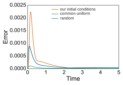
Refer to caption
Figure 9: The error ϵ(n)italic-ϵ𝑛\epsilon(n) for n=17𝑛17n=17 for the PA lumped equations considering different initial conditions.

References

  • Albert and Barabási (2002) R. Albert and A.-L. Barabási, Reviews of Modern Physics 74, 47 (2002).
  • Newman (2003) M. E. Newman, SIAM Review 45, 167 (2003).
  • Strogatz (2001) S. H. Strogatz, nature 410, 268 (2001).
  • Palla et al. (2005) G. Palla, I. Derenyi, I. Farkas,  and T. Vicsek, Nature 435, 814 (2005).
  • Boccaletti et al. (2006) S. Boccaletti, V. Latora, Y. Moreno, M. Chavez,  and D.-U. Hwang, Physics Reports 424, 175 (2006).
  • Barrat et al. (2008) A. Barrat, M. Barthlemy,  and A. Vespignani, Dynamical Processes on Complex Networks. (Cambridge University Press, 2008).
  • Dorogovtsev et al. (2008) S. N. Dorogovtsev, A. V. Goltsev,  and J. F. Mendes, Reviews of Modern Physics 80, 1275 (2008).
  • Pastor-Satorras et al. (2015) R. Pastor-Satorras, C. Castellano, P. Van Mieghem,  and A. Vespignani, Reviews of Modern Physics 87, 925 (2015).
  • Gross et al. (2006) T. Gross, C. J. D. DLima,  and B. Blasius, Physical review letters 96, 208701 (2006).
  • Gross and Blasius (2008) T. Gross and B. Blasius, Journal of the Royal Society Interface 5, 259 (2008).
  • Marceau et al. (2010) V. Marceau, P.-A. Noël, L. Hébert-Dufresne, A. Allard,  and L. J. Dubé, Physical Review E 82, 036116 (2010).
  • Van Segbroeck et al. (2010) S. Van Segbroeck, F. C. Santos,  and J. M. Pacheco, PLoS Computational Biology 6, e1000895 (2010).
  • Wu et al. (2012) Q. Wu, X. Fu, M. Small,  and X.-J. Xu, Chaos: an interdisciplinary journal of nonlinear science 22, 013101 (2012).
  • Wang et al. (2015) Z. Wang, M. A. Andrews, Z.-X. Wu, L. Wang,  and C. T. Bauch, Physics of Life Reviews 15, 1 (2015).
  • Mata et al. (2014) A. S. Mata, R. S. Ferreira,  and S. C. Ferreira, New Journal of Physics 16, 053006 (2014).
  • Gómez et al. (2011) S. Gómez, J. Gómez-Gardenes, Y. Moreno,  and A. Arenas, Physical Review E 84, 036105 (2011).
  • Juhász et al. (2012) R. Juhász, G. Ódor, C. Castellano,  and M. A. Muñoz, Physical Review E 85, 066125 (2012).
  • Boguñá et al. (2009) M. Boguñá, C. Castellano,  and R. Pastor-Satorras, Physical Review E 79, 036110 (2009).
  • Lee et al. (2013) H. K. Lee, P.-S. Shim,  and J. D. Noh, Physical Review E 87, 062812 (2013).
  • Didier et al. (2009) F. Didier, T. A. Henzinger, M. Mateescu,  and V. Wolf, in High Performance Computational Systems Biology, 2009. HIBI’09. International Workshop on (IEEE, 2009) pp. 118–127.
  • Wolf et al. (2010) V. Wolf, R. Goel, M. Mateescu,  and T. A. Henzinger, BMC Systems Biology 4, 42 (2010).
  • Bortolussi et al. (2013) L. Bortolussi, J. Hillston, D. Latella,  and M. Massink, Performance Evaluation 70, 317 (2013).
  • Pastor-Satorras and Vespignani (2001) R. Pastor-Satorras and A. Vespignani, Physical Review Letters 86, 3200 (2001).
  • Gleeson (2011) J. P. Gleeson, Physical Review Letters 107, 068701 (2011).
  • Cator and Van Mieghem (2012) E. Cator and P. Van Mieghem, Physical Review E 85, 056111 (2012).
  • Mata and Ferreira (2013) A. S. Mata and S. C. Ferreira, EPL (Europhysics Letters) 103, 48003 (2013).
  • Demirel et al. (2014) G. Demirel, F. Vazquez, G. Böhme,  and T. Gross, Physica D: Nonlinear Phenomena 267, 68 (2014).
  • Castellano and Pastor-Satorras (2010) C. Castellano and R. Pastor-Satorras, Physical Review Letters 105, 218701 (2010).
  • Gleeson et al. (2012) J. P. Gleeson, S. Melnik, J. A. Ward, M. A. Porter,  and P. J. Mucha, Physical Review E 85, 026106 (2012).
  • Gleeson (2013) J. P. Gleeson, Physical Review X 3, 021004 (2013).
  • Fennell (2015) P. G. Fennell, Stochastic processes on complex networks: techniques and explorationsPh.D. thesis, University of Limerick (2015).
  • Broder et al. (2000) A. Broder, R. Kumar, F. Maghoul, P. Raghavan, S. Rajagopalan, R. Stata, A. Tomkins,  and J. Wiener, Computer networks 33, 309 (2000).
  • Newman (2001) M. E. Newman, Proceedings of the National Academy of Sciences 98, 404 (2001).
  • Clauset et al. (2009) A. Clauset, C. R. Shalizi,  and M. E. Newman, SIAM Review 51, 661 (2009).
  • Wright and Nocedal (1999) S. Wright and J. Nocedal, Springer Science 35, 67 (1999).
  • LUMPY Tool (2017) LUMPY Tool, https://mosi.uni-saarland.de/lumpy (2017).
  • Miller and Volz (2013) J. C. Miller and E. M. Volz, PloS One 8, e69162 (2013).
  • Pilcher et al. (2004) C. D. Pilcher, H. C. Tien, J. J. Eron, P. L. Vernazza, S.-Y. Leu, P. W. Stewart, L.-E. Goh,  and M. S. Cohen, Journal of Infectious Diseases 189, 1785 (2004).
  • Eames and Keeling (2002) K. T. Eames and M. J. Keeling, Proceedings of the National Academy of Sciences 99, 13330 (2002).
  • Liljeros et al. (2001) F. Liljeros, C. R. Edling, L. A. N. Amaral, H. E. Stanley,  and Y. Åberg, Nature 411, 907 (2001).