Multi-scale streaming anomalies detection for time series

Résumé

In the class of streaming anomaly detection algorithms for univariate time series, the size of the sliding window over which various statistics are calculated is an important parameter. To address the anomalous variation in the scale of the pseudo-periodicity of time series, we define a streaming multi-scale anomaly score with a streaming PCA over a multi-scale lag-matrix. We define three methods of aggregation of the multi-scale anomaly scores. We evaluate their performance on Yahoo! and Numenta dataset for unsupervised anomaly detection benchmark. To the best of authors’ knowledge, this is the first time a multi-scale streaming anomaly detection has been proposed and systematically studied.

Mots-clef: Multi-scale, Anomaly detection, Streaming, PCA

1 Introduction

Anomalies in time series are defined as points which deviate in a significant way from a certain model. For instance this can be the deviation from the local mean value of the time series. Anomaly detection is an important problem in industrial process control and for biomedical applications. There are few common methods used in the detection of anomalies once we define the representation of the time series at each point. One can either look at the distribution of the distances of the k-nearest neighbour of a given point  [BKNS00], which basically measures for relative density of neighbours around a point. One can evaluate the errors of prediction in auto-regressive models [LAF15] which models the predicted value as a linear function of the past. Finally one could reconstruct the input point or vector while tracking the principal subspace  [PSF05], this helps locate the dominant pattern in a time series.

Streaming anomaly detection consists of detecting anomalies on the fly, where one has access only to the current time sample and all its past values at any time. This is frequently applicable to large data processing requirements at each time instant, that storing models or representations of these signals are not feasible. Algorithms designed for streaming should update their parameters on the arrival of each new point so as to adapt to changes in the time series.

A point anomaly is the value of the time series which deviates from the rest of the time series. An anomalous pattern is a window of values of that deviates from the rest of the windows of the time series. One can also note that the point anomaly is also a anomaly pattern when the window is point sized.

Multiscale Anomalies

Given different time series we aim to take into account the variation in the window sizes at which anomaly patterns occur in the series. In this paper we address the problem of designing a multiscale streaming anomaly detector. We also study the multiscale approximation of the the moving window of the time series by the haar wavelet transformation. The second goal is to study the effect principal subspace tracking over the haar basis.

Figure 1: Example input time series and their corresponding lag-matrices $X_{t}^{p}$ for different scales of moving window $p=2,4,6,8,32$. The multi-scale streaming PCA evaluates the principal subspace at each scale $p$. The reconstruction error across all scales $p$ gives the final multi-scale anomaly score $\boldsymbol{\alpha}_{t}$.

Previous work

[LAF15] proposed several linear predictive models (Autoregressive, Kalman filter) followed by an anomaly score filtering (by $k\sigma$ rule, or local outlier factor scores introduced by [BKNS00]) to detect anomalies. The authors also published a dataset to evaluate unsupervised anomaly detectors on real and synthetic data. This is for off-line time series data though we shall use the annotations available to evaluate the anomaly detection performance.

The Numenta Anomaly Benchmark (NAB) [LA15] provides an evaluation of streaming time series anomaly detection algorithms. The algorithms include hierarchical temporal memory, Twitter Advec and Skyline, each of which individually are anomaly detection packages. We shall not evaluate within the NAB benchmark for the moment, but we are planning a detailed evaluation in the future. [CD15] provides an overview of incrementally calculate principal components, while also discussing the choice of learning rate parameter. [dSTM10] use a streaming subspace tracking algorithm that provides a rank adaptive and numerically stable streaming PCA algorithm for anomaly detection.

There are two studies closest to our work : Firstly [PY06] evaluate a multiscale streaming PCA to extract the most “representative” window from an lag-embedding of an univariate time series for different window sizes. The algorithm was used to track correlations at multiple scales. While [CZ08] perform multiscale anomaly detection by searching for infrequent windows in the input time series, they do not evaluate anomalies on-line.

There has also been recent work in the evaluation of on-line empirical mode decomposition (EMD) paper [FBF17] which evaluates the empirical modes in streaming. There has also been recent work on use matrix sketching to approximate wavelet coefficients in a streaming set up [CGS06].

2 Background and Notations

Notations

: The univariate time series are denoted by $x(t)$, and $T$ denotes the number of samples, and $p$ the lag window size. We embed the window of past $p$ values of the univariate time series to construct a $p$-dimensional sample $X_{t}^{p}$ of the multivariate time series:

$$X_{t}^{p}=[x_{t},x_{t-1},\ldots,x_{t-p+1}]^{T}\in\mathbb{R}^{p}$$ (1)

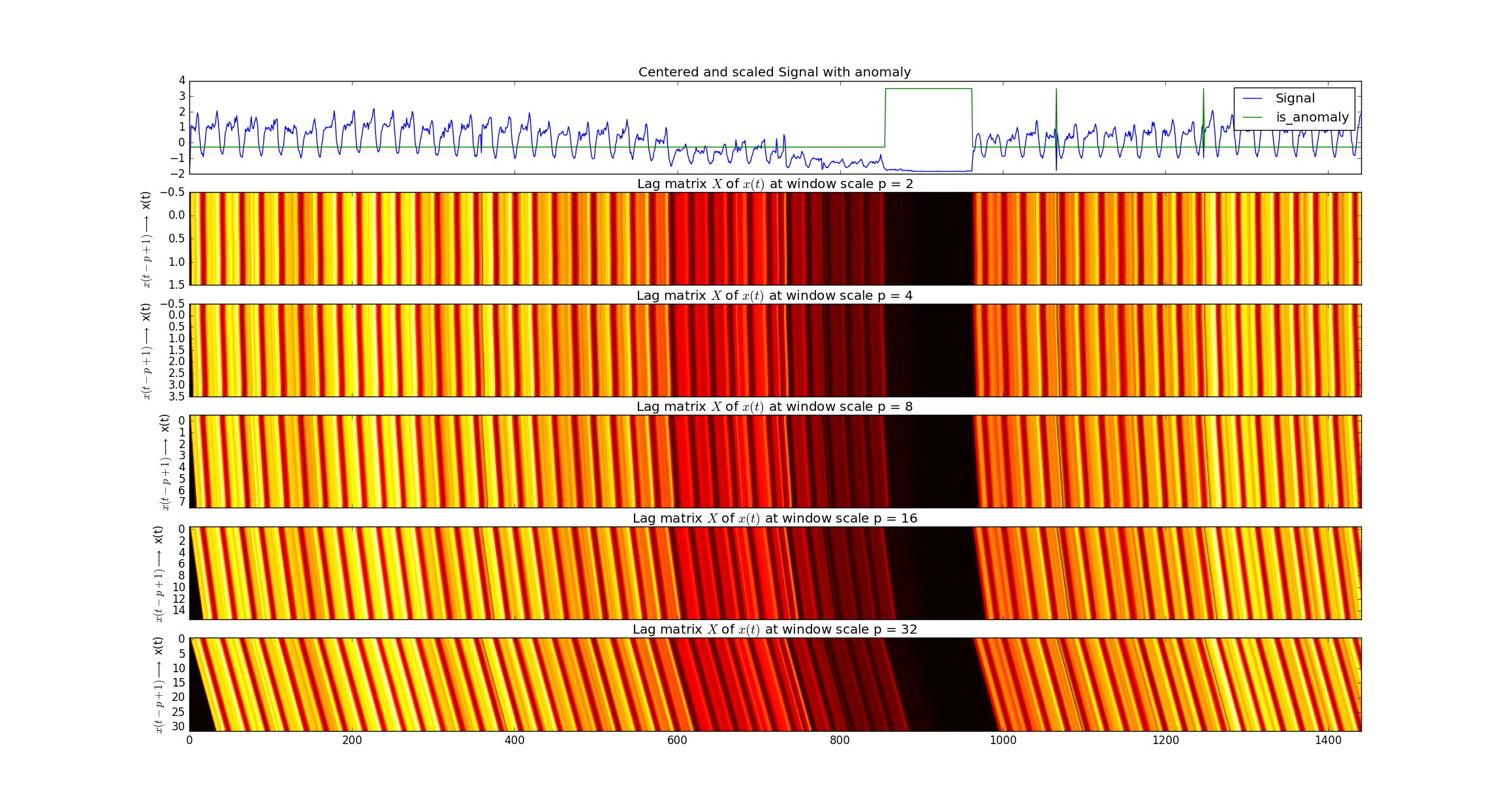
When $t<p$, the missing values in $X_{t}^{p}$ repeat most recent time sample. The vectors are stacked in a matrix $X^{p}\in\mathbb{R}^{T\times p}$. In a multi-scale setting, we will often consider multiple window sizes $\{p_{j}\}^{J}_{j=1}$ with $p_{j}=2^{j}$ depending on the case. To simplify notations we write $X_{t}^{j}$ to denote $X_{t}^{p_{j}}$. This enables us to denote a family of geometrically increasing lag-windows with a parameter $j\in 1,2,...J$ where $J$ refers to the largest scale. An example time series with the corresponding lag-matrix is shown in figure 1.

Figure 2: Evolution of the principal direction and the point cloud for a 2-dimensional lagmatrix. The color scale shown below represents (viewed from left to right) the direction of time. The black line in each plot represents the principal direction at that time instant $t$. One should also note that the direction is adapted even to anomalous points since they are never known in advance. This might lead to increased false positives.

We focus on a class of methods relying on the online estimation of the principal component of the lag-matrix, pioneered by [PSF05]. The anomaly score is then simply derived as the reconstruction error. For simplicity, we only consider the first principal direction.

Given a design matrix $X^{p}\in\mathbb{R}^{T\times p}$, the first principal direction $\mathbf{w}_{p}$ is defined as the 1-D projection capturing most of the energy of the data samples :

$$\mathbf{w}_{p}=\arg\min_{\|\mathbf{w}\|=1}\sum^{T}_{t=1}\|X_{t}^{p}-(\mathbf{w}\mathbf{w}^{T})X_{t}^{p}\|^{2}$$ (2)

We solve this problem in an online fashion following the approach of [PSF05]. For a given scale  [PSF05] use the projective approximation subspace tracking algorithm (PAST) first introduced in  [Yan95]. For the formal proofs of convergence to the true principal subspace projection, we refer you to a good review provided by [LM05]. An adapted version of this method can be read in Algorithm 1.

At time $t$, we denote by $\widetilde{X}_{t}^{p}$ the projection of $X_{t}^{p}$ upon $\mathbf{w}^{p}$ (at this time step), i.e. $\widetilde{X}_{t}^{p}=\mathbf{w}_{p}^{T}X_{t}^{p}$. The anomaly score at time $t$ and for a window of size $p$ will be written as $\alpha_{t}^{p}=\|\widetilde{X}_{t}^{p}-X_{t}^{p}\|^{2}$. When considering dyadic windows $p_{j}$, we also write $\mathbf{w}_{p_{j}}=:\mathbf{w}_{j}$ and $\alpha^{p_{j}}=:\alpha^{j}$.

3 Streaming anomaly detection

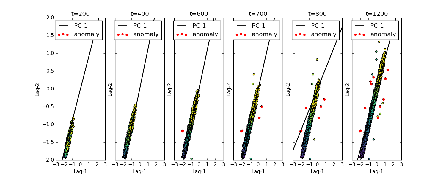
In this section we propose two algorithms for anomaly detection. They develop on the Streaming PCA and Hierarchical PCA algorithms developed for optimal pattern extraction in time series, and apply them to the problem of anomaly detection, while being more amenable to multiple scales. We show an example of the application of the streaming PCA algorithm in figure 2 at scale=2. In this example the lagmatrix has 2-dimensions that can be visualized in a plane. We see the evolution of the principal direction with new incoming points. It is important to note that for each new incoming point, we project it and its $p-1$ past samples, i.e. $X_{t}^{p}$ onto the current principal direction $\mathbf{w}_{p}$ and adapt the direction so as to reduce the error of reconstruction. This is not a prediction. $\mathbf{w}_{p}\mathbf{w}_{p}X_{t}^{p}$ captures the largest amount of variance in the time series. The number of principal directions determine the degrees of independent variation in the time series.

3.1 Multiscale Streaming PCA

The streaming PCA algorithm introduced by [PSF05] consists in computing an online PCA on the past lags of the time series $X^{j}$. We use the subsequent reconstruction error as an anomaly score. Throughout this paper, we only consider the first PCA direction, though it is a straightforward extension to consider the first $k$ PCA directions.

A natural extension of this algorithm to a multiscale setting would consist in computing simultaneously the PCA directions at multiple scales $p_{j}=2^{j}$ for $j\geq 1$ up to a maximal scale $P=2^{J}$. The main drawback of this extension is its time complexity. Indeed, for a past window of size $p_{j}$, the streaming PCA algorithm requires $\mathcal{O}(Tp_{j})$ operations to attribute an anomaly score on a time series of length $T$. This multiscale extension would therefore require $\mathcal{O}(TP)$, which can be prohibitive for $P$ large. This is introduced in algorithm 1.

Initialization: $\mathbf{w}_{j}\leftarrow\mathbf{0}$, $\sigma_{j}^{2}\leftarrow\epsilon$ with $\epsilon\ll 1$ for $t=1,\ldots,T$ do     for $j=1,\ldots,J$ do          $Z_{t}^{j}\leftarrow H_{2^{j}}^{T}X_{t}^{j}$          $y^{j}_{t}\leftarrow\mathbf{w}_{j}^{T}X_{t}^{j}$          $\sigma_{j}^{2}\leftarrow\sigma_{j}^{2}+(y_{t}^{j})^{2}$          $\mathbf{e}_{t}^{j}\leftarrow Z_{t}^{j}-y_{t}^{j}\mathbf{w}_{j}$          $\mathbf{w}_{j}\leftarrow\mathbf{w}_{j}+\sigma_{j}^{-2}y_{t}^{j}\mathbf{e}_{t}^{j}$          $\pi_{t}^{j}\leftarrow\mathbf{w}_{j}^{T}Z_{t}^{j}$          $\widetilde{Z}_{t}^{j}\leftarrow\pi_{t}^{j}\mathbf{w}_{j}$          $\alpha_{t}^{j}\leftarrow\|\widetilde{Z}_{t}^{j}-Z_{t}^{j}\|^{2}$     end for end for return $\boldsymbol{\alpha}\in\mathbb{R}^{T\times J}$ Algorithm 1 Multiscale streaming PCA

3.2 Hierarchical streaming PCA

Initialization: $\mathbf{w}_{j}\leftarrow\mathbf{0}$, $\sigma_{j}^{2}\leftarrow\epsilon$ with $\epsilon\ll 1$ for $t=1,\ldots,T$ do     for $j=2,\ldots,J$ do          if $j=1$ then              $Z_{t}^{j}\leftarrow H_{2^{j}}^{T}X_{t}^{j}$          else              $Z_{t}^{j}\leftarrow[\pi_{t}^{j-1},(Z_{t}^{j})^{T}]$          end if          $y_{t}^{j}\leftarrow\mathbf{w}_{j}^{T}Z_{t}^{j}$          $\sigma_{j}^{2}\leftarrow\sigma_{j}^{2}+(y_{t}^{j})^{2}$          $\mathbf{e}_{t}^{j}\leftarrow Z_{t}^{j}-y_{t}^{j}\mathbf{w}_{j}$          $\mathbf{w}_{j}\leftarrow\mathbf{w}_{j}+\sigma_{j}^{-2}y_{t}^{j}\mathbf{e}_{t}^{j}$          $\pi_{t}^{j}\leftarrow\mathbf{w}_{j}^{T}Z_{t}^{j}$          $\widetilde{Z}_{t}^{j}\leftarrow\pi_{t}^{j}\mathbf{w}_{j}$          $\alpha_{t}^{j}\leftarrow\|\widetilde{Z}_{t}^{j}-Z_{t}^{j}\|^{2}$     end for end for return $\boldsymbol{\alpha}\in\mathbb{R}^{T\times J}$ Algorithm 2 Hierarchical streaming PCA

Figure 3: Hierarchical Streaming PCA.

To overcome redundant calculation in the multiscale streaming PCA algorithm [PY06] introduced a hierarchical approximation, sketched in Figure 3 and algorithm 2. When passing from one scale $p_{j}$ to the next $p_{j+1}=2p_{j}$, instead of rebuilding the lag matrix $X_{t}^{j+1}$ whose size doubles, it builds a reduced lag matrix $Z_{t}^{j+1}$ by considering the projection of each component of size $p_{j}$ on the principal direction obtained at this scale, i.e. $Z_{t}^{j+1}=[\mathbf{w}^{T}_{j}Z_{t}^{j},\mathbf{w}^{T}_{j}Z_{t-2^{j}}^{j}]^{T}$ with $Z_{t}^{1}=X_{t}^{1}$. The principal direction at scale $p_{j+1}$ is then obtained by applying the streaming PCA algorithm on this reduced representation. Note that the reconstruction error at each scale is only relative to the previous scale, and we do not back-propagate to the finest scale of the actual time series. In some sense, this approach can be seen as a linear convolutional neural network (CNN).

Figure 4: Schematic representation of the proposed method and different multi-scale anomaly score aggregation methods. After the construction of an adapted representation of the lag matrix at multiple scales, which can be done in a hierarchical manner (indicated by the dotted arrows), anomaly scores are obtained for each scale and then recombined to obtain a final score.

Figure 5: Haar basis for time series length N=8.

Figure 6: Example time series in blue with the anomalies market in green (left). The errors of reconstruction (right) at different geometric scales. The reconstruction error for the change of basis with the haar transform is also plotted. The reconstruction error of the haar coefficients produces a shared peak in error compared in the reconstruction error of the naive lag-matrix.

The main assumption underlying this approach is that at each change of scale, the projection at the previous scale is equally valid for the near past (first half at scale $p_{j}$) and the far past (second half at scale $p_{j}$). In the context of streaming anomaly detection, we argue that this assumption is not necessarily relevant. Yet, the benefits of the hierarchy for run-time complexity should not be ignored: the Hierarchical PCA algorithm takes $\mathcal{O}(T\log P)$ operations to run up to scale $P$, where $P=2^{J}$.

Haar transform :

The haar transform is a multiscale approximation of an input time series window $X_{t}^{p}$ at of window size N=$2^{p}$ can be calculated by the dot product with the haar basis. The unitary haar basis are calculated by the following recursion equation with $H_{1}=[1]$ :

$$H_{2N}={\frac{1}{\sqrt{2}}\begin{bmatrix}H_{N}\otimes[1,1]\\ I_{N}\otimes[1,-1]\end{bmatrix}}$$ (3)

The haar basis for a time series of length $N=4$ is given by :

$$H_{4}={\frac{1}{2}}{\begin{bmatrix}1&1&1&1\\ 1&1&-1&-1\\ \sqrt{2}&-\sqrt{2}&0&0\\ 0&0&\sqrt{2}&-\sqrt{2}\end{bmatrix}}$$ (4)

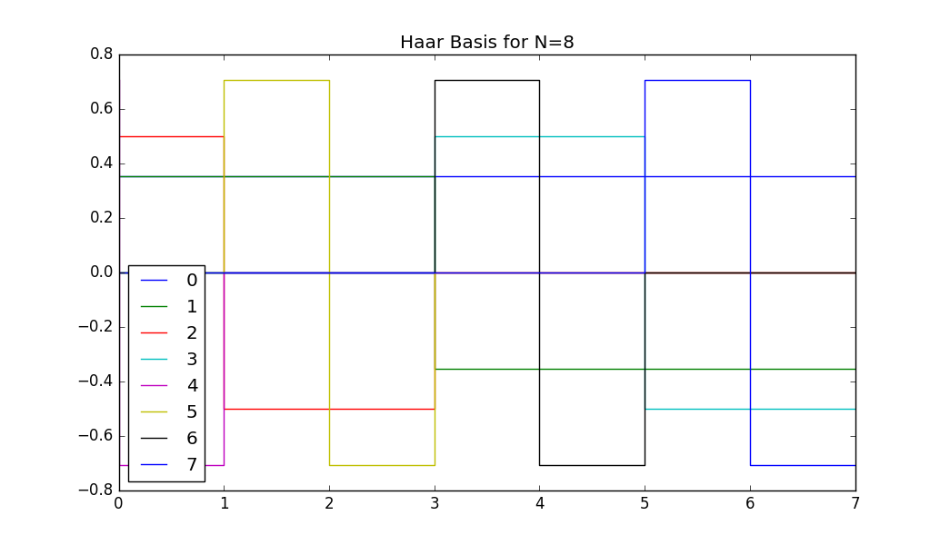
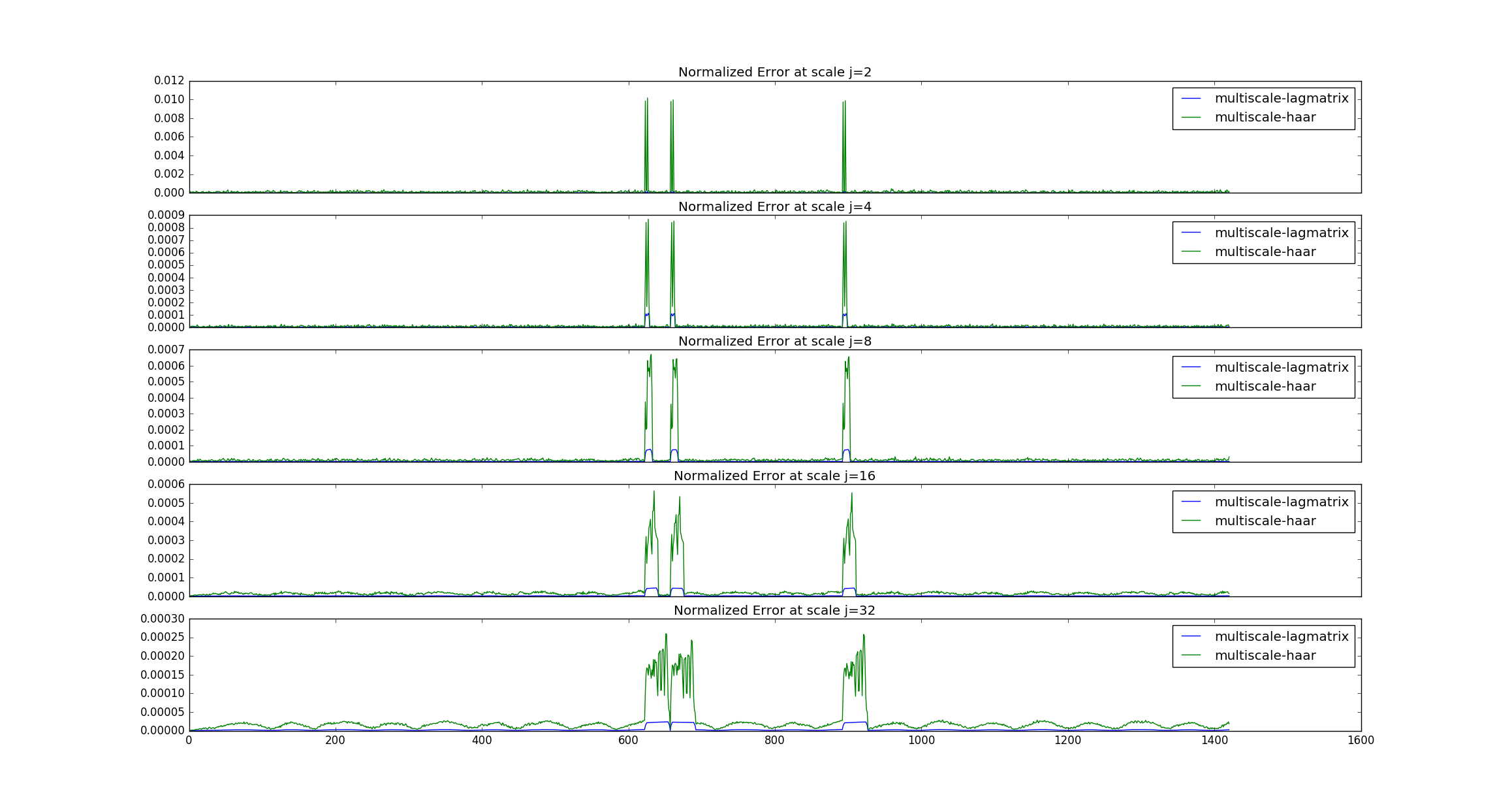
For each lag window $X_{t}^{p}$ we perform a change of basis using the unitary Haar transform $H^{T}X_{t}^{p}$. This provides a representation of the time series that is well known in wavelet analysis to approximate signals, the basis are shown in figure 5. In this study we simply use the complete change of basis to understand its effect on the reconstruction error. We observe in figure 6, an relatively sharper spike in error at the anomaly for a change of basis using the Haar basis, as compared to a regular multiscale lagmatrix reconstruction. In future work we aim to perform the Haar decomposition in streaming and perform a reconstruction of the time series, without evaluating the principal subspace.

The final flow of operations per time sample is demonstrated in figure 4. The hierarchical approximation is not shown, but basically consists again in calculating the reconstruction error of the multi-scale lagmatrix. The table 1 gives the time complexity for the streaming PCA algorithm as well as it’s hierarchical approximation.

Algorithm	Multiscale PCA	Hierarchical PCA
Complexity	$\mathcal{O}(TP)$	$\mathcal{O}(T\log{}P)$

Table 1: Number of floating point operations of streaming PCA for multiscale methods on a time series of length $T$ up to a maximal window size $P$.

4 Experiments

In this section we evaluate the performance of the different time series representations for the streaming PCA based multiscale anomaly detector. In this light we also propose three different ways of deciding the final score given an input anomaly score at multiple scales $\boldsymbol{\alpha}_{t}=\{\alpha_{t}^{j}\}_{j\leq J}$. Namely, we evaluate the following aggregations:

1. $\|\boldsymbol{\alpha}_{t}\|^{2}$ : Norm of multiscale anomaly score

2. $\|\widetilde{\boldsymbol{\alpha}_{t}}-\boldsymbol{\alpha}_{t}\|^{2}$: Streaming reconstruction error on anomaly score, obtained via a 2nd iteration of the streaming PCA algorithm on the multiscale anomaly score instead of the lag-matrix.

3. $\alpha_{t}^{j^{\ast}}$ where $j^{\ast}={\arg\min}_{j}\sum_{i}(\boldsymbol{\alpha}^{T}\boldsymbol{\alpha})_{ji}$ : the anomaly score corresponding to the scale which is least correlated with others.

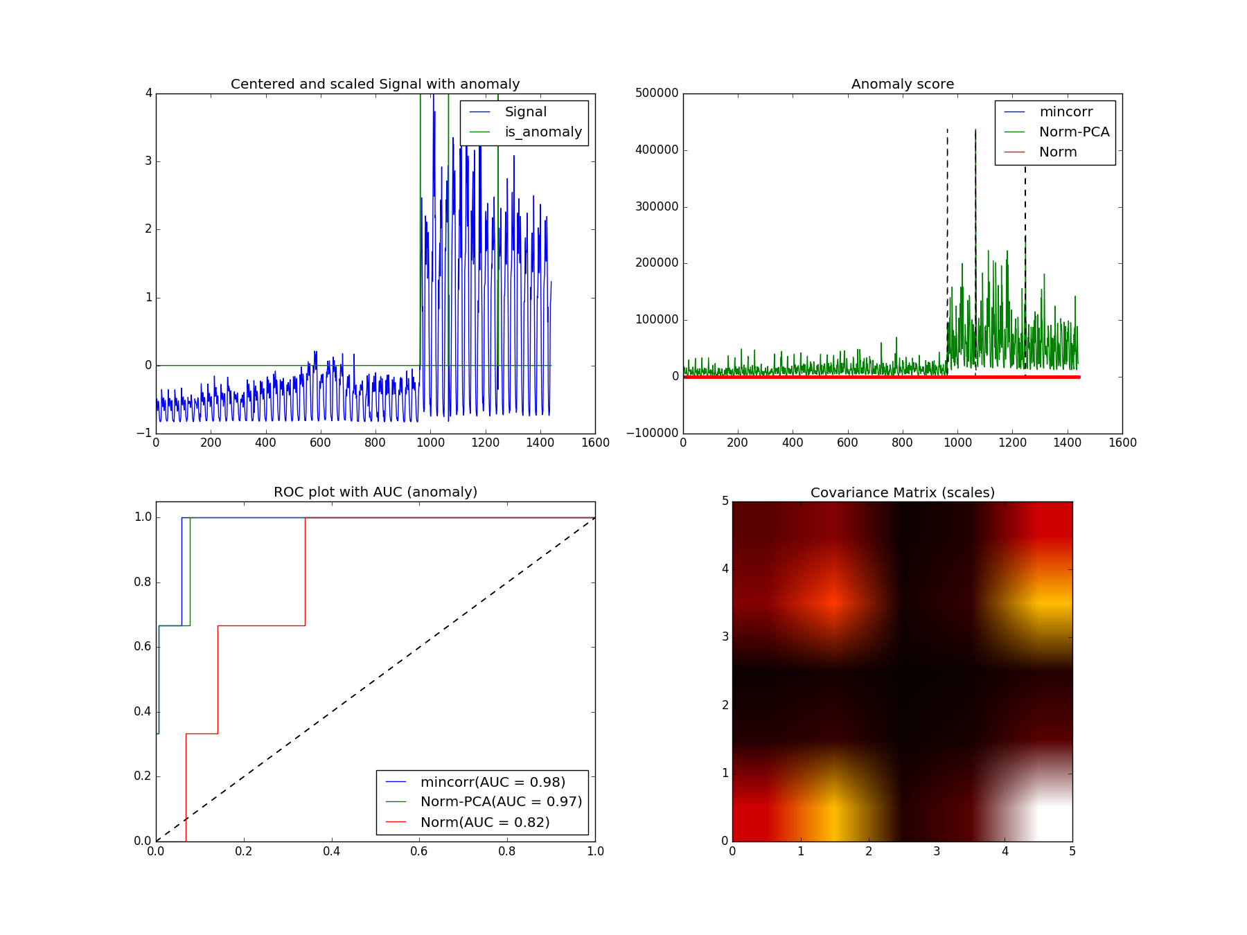
To assess the performance of a detector, we use the area under the receiver operators characteristics curve (AUC), which is calculated by integrating the curve of the False positive rate(FPR) vs the True positive rate (TPR) obtained for all possible thresholds. This AUC score is comprised between $0,1$ where $0.5$ corresponds to the worst value, that is detection is equivalent to random guessing while $1$ or $0$ is a perfect detector or perfect rejection. In the plot of AUC for individual time series we plot the AUC=0.5 in dotted lines to remark the location of random guessing. We evaluate the AUC for each time series in each benchmark and provide the mean value with its standard deviation for the AUC’s of the time series in each benchmark.

The work in  [LAF15] evaluates off-line models and do not consider a streaming anomaly detection setup. While [LA15] is expressly created for streaming anomaly detection time series, though we do not report an explicit comparison with their scores in this study which would consist of evaluating in the NAB platform. But we do plan for a complete evaluation in the future. All code will be soon available online.

Dataset description: In our study we use the Yahoo! time series dataset introduced by [LAF15]. It consists of four different datasets (Benchmark $1$ to $4$), each of them containing approximately $100$ time series. Benchmark 1 contains real time series data from Yahoo! traffic data, which are time series with a variety of different scales of repeating patterns, and is the most difficult benchmark to detect anomalies. Benchmarks 2 and 3 have synthetic time series which are mainly sinusoids with varying frequencies and varying levels of noise with relatively easier to detect anomalies. Benchmark 4 contains non-stationary artificial time series with oscillations and linear trends, containing not only anomalies but change-points. Change-points are not evaluated in this study. Finally the Numenta anomaly detection dataset [LA15] like benchmark 4, contains synthetic and real time series with hard-to-detect examples.

Observations

: The results of evaluation of the multiscale streaming PCA, and the hierarchical approximation is reported in table 2. Each benchmark consists of 70-100 series, we report the median value of the AUC values across the benchmark. We also report the deviation of the AUC scores across their median (Median absolute deviation). Given the multiscale anomaly scores $\boldsymbol{\alpha}_{t}$ we evaluate the performance of the three ways to aggregate the multi-scale score : $\|\boldsymbol{\alpha}_{t}\|^{2},\|\widetilde{\boldsymbol{\alpha}_{t}}-\boldsymbol{\alpha}_{t}\|^{2}$ and $\alpha_{t}^{j^{\ast}}$, namely the norm, iterated streaming PCA on the multiscale score $\|\boldsymbol{\alpha}_{t}\|^{2}$ and finally the least correlated scale. We also evaluate the performance when tracking only the first principal subspace (PC=1), and that for the first two subspaces (PC=2), to observe the effect of preserving more variance. Finally we tracked the principal subspace of a single scale naive lag-matrix at one scale, to compare it’s performance w.r.t a multi-scale approach.

In all benchmarks, the multi-scale anomaly scores perform better than their single scale counterpart. An important empirical result is the effect of de-correlation between scales. We see that w.r.t the norm of the multi-scale score the least correlated scale performs better on almost all benchmarks. This effect is also reflected in the usage of a 2nd-iteration of the streaming PCA on the multi-scale anomaly score, whose reconstruction error norm represents the projections that are orthogonal to the principal direction across all scales.

Except for Benchmark $1$ where considering the norm of all anomaly scores appears to provide the best results, running another streaming PCA on top of these scores appears to be the best way to achieve good results. We also observe that the increase in the number of principal components do not improve the performance of the detector.

Failure cases

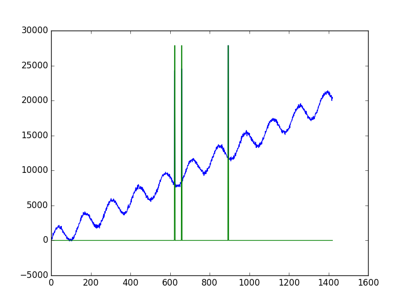
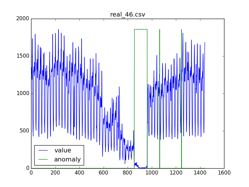
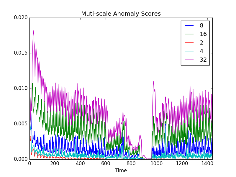
In figure 8 we have a time series whose anomalous window is a one whose value drops. Reconstruction at different scales are produce good approximations and no observable increase in errors, and thus anomaly score. In such situations a non-linear function such as a minimum of moving window would have detected the anomaly.

Figure 7: Time series with the three different final anomaly scores : Norm $\|\boldsymbol{\alpha}_{t}\|^{2}$, Norm-PCA $\|\widetilde{\boldsymbol{\alpha}_{t}}-\boldsymbol{\alpha}_{t}\|^{2}$ (2nd iteration of PCA), MinCorr / least correlated scale $\alpha_{t}^{j^{\ast}}$ where $j^{\ast}={\arg\min}\leavevmode\nobreak\ \sum_{i}(\boldsymbol{\alpha}^{T}\boldsymbol{\alpha})_{ji}$. We also plot the covariance of the norm of the errors between different scales. The decorrelation in reconstruction errors across the different scales, in our study, produces a robust detection of anomalies.

Multi-scale score-Norm $\|\boldsymbol{\alpha}_{t}\|^{2}$ (PC=1)
Method / AUCs	Bench 1	Bench 2	Bench 3	Bench 4	NAB
fixed-scale	$0.828\pm 0.240$	$0.835\pm 0.180$	$0.614\pm 0.108$	$0.568\pm 0.160$	$0.815\pm 0.238$
fixed-scale-haar	$0.826\pm 0.238$	$0.878\pm 0.143$	$0.617\pm 0.115$	$0.576\pm 0.157$	$0.812\pm 0.232$
multiscale-lagmatrix	$0.884\pm 0.232$	$0.978\pm 0.057$	$0.816\pm 0.092$	$0.696\pm 0.157$	$0.879\pm 0.199$
hierarchical-approx	$0.871\pm 0.236$	$0.997\pm 0.002$	$0.980\pm 0.025$	$0.897\pm 0.104$	$0.900\pm 0.189$
multiscale-haar	$0.906\pm 0.231$	$0.989\pm 0.019$	$0.992\pm 0.019$	$0.892\pm 0.126$	$0.892\pm 0.198$
Multi-scale score-Norm $\|\boldsymbol{\alpha}_{t}\|^{2}$ (PC=2)
fixed-scale	$0.783\pm 0.269$	$0.918\pm 0.065$	$0.616\pm 0.142$	$0.569\pm 0.154$	$0.815\pm 0.231$
fixed-scale-haar	$0.808\pm 0.259$	$0.925\pm 0.074$	$0.627\pm 0.146$	$0.586\pm 0.144$	$0.811\pm 0.232$
multiscale-lagmatrix	$0.850\pm 0.242$	$0.969\pm 0.031$	$0.803\pm 0.116$	$0.686\pm 0.163$	$0.862\pm 0.210$
hierarchical-approx	$0.848\pm 0.240$	$0.985\pm 0.056$	$0.982\pm 0.021$	$0.941\pm 0.079$	$0.876\pm 0.213$
multiscale-haar	$0.862\pm 0.245$	$0.976\pm 0.021$	$0.805\pm 0.150$	$0.710\pm 0.166$	$0.873\pm 0.195$
PCA on multi-scale score $\|\widetilde{\boldsymbol{\alpha}_{t}}-\boldsymbol{\alpha}_{t}\|^{2}$ (PC=1)
Method / AUCs	Bench 1	Bench 2	Bench 3	Bench 4	NAB
fixed-scale	$0.632\pm 0.264$	$0.754\pm 0.206$	$0.533\pm 0.124$	$0.525\pm 0.133$	$0.700\pm 0.247$
fixed-scale-haar	$0.649\pm 0.251$	$0.723\pm 0.194$	$0.514\pm 0.110$	$0.522\pm 0.129$	$0.699\pm 0.244$
multiscale-lagmatrix	$0.895\pm 0.218$	$0.997\pm 0.006$	$0.993\pm 0.017$	$0.959\pm 0.063$	$0.891\pm 0.194$
hierarchical-approx	$0.859\pm 0.233$	$0.997\pm 0.002$	$0.961\pm 0.071$	$0.895\pm 0.108$	$0.884\pm 0.204$
multiscale-haar	$0.888\pm 0.219$	$0.988\pm 0.031$	$0.956\pm 0.059$	$0.898\pm 0.106$	$0.886\pm 0.178$
PCA on multi-scale score $\|\widetilde{\boldsymbol{\alpha}_{t}}-\boldsymbol{\alpha}_{t}\|^{2}$ (PC=2)
fixed-scale	$0.778\pm 0.270$	$0.908\pm 0.091$	$0.609\pm 0.133$	$0.573\pm 0.154$	$0.813\pm 0.232$
fixed-scale-haar	$0.804\pm 0.261$	$0.922\pm 0.079$	$0.625\pm 0.148$	$0.584\pm 0.143$	$0.811\pm 0.232$
multiscale-lagmatrix	$0.828\pm 0.237$	$0.872\pm 0.134$	$0.834\pm 0.172$	$0.793\pm 0.181$	$0.829\pm 0.207$
hierarchical-approx	$0.831\pm 0.248$	$0.978\pm 0.084$	$0.976\pm 0.031$	$0.935\pm 0.084$	$0.841\pm 0.231$
multiscale-haar	$0.816\pm 0.239$	$0.933\pm 0.088$	$0.859\pm 0.161$	$0.799\pm 0.171$	$0.807\pm 0.226$
Least correlated scale $\alpha_{t}^{j^{\ast}}$ where $j^{\ast}={\arg\min}_{j}\sum_{i}(\boldsymbol{\alpha}^{T}\boldsymbol{\alpha})_{ji}$ (PC=1)
Method / AUCs	Bench 1	Bench 2	Bench 3	Bench 4	NAB
fixed-scale	$0.828\pm 0.240$	$0.835\pm 0.180$	$0.614\pm 0.108$	$0.568\pm 0.160$	$0.815\pm 0.238$
fixed-scale-haar	$0.826\pm 0.238$	$0.878\pm 0.143$	$0.617\pm 0.115$	$0.576\pm 0.157$	$0.812\pm 0.232$
multiscale-lagmatrix	$0.816\pm 0.238$	$0.773\pm 0.236$	$0.993\pm 0.017$	$0.964\pm 0.055$	$0.885\pm 0.196$
hierarchical-approx	$0.816\pm 0.238$	$0.773\pm 0.236$	$0.993\pm 0.017$	$0.964\pm 0.055$	$0.885\pm 0.196$
multiscale-haar	$0.832\pm 0.238$	$0.997\pm 0.007$	$0.799\pm 0.120$	$0.817\pm 0.123$	$0.886\pm 0.183$
Least correlated scale $\alpha_{t}^{j^{\ast}}$ where $j^{\ast}={\arg\min}_{j}\sum_{i}(\boldsymbol{\alpha}^{T}\boldsymbol{\alpha})_{ji}$ (PC=2)
fixed-scale	$0.783\pm 0.269$	$0.918\pm 0.065$	$0.616\pm 0.142$	$0.569\pm 0.154$	$0.815\pm 0.231$
fixed-scale-haar	$0.808\pm 0.259$	$0.925\pm 0.074$	$0.627\pm 0.146$	$0.586\pm 0.144$	$0.811\pm 0.232$
multiscale-lagmatrix	$0.685\pm 0.332$	$0.757\pm 0.225$	$0.555\pm 0.140$	$0.597\pm 0.168$	$0.736\pm 0.327$
hierarchical-approx	$0.689\pm 0.333$	$0.757\pm 0.225$	$0.555\pm 0.140$	$0.596\pm 0.167$	$0.736\pm 0.327$
multiscale-haar	$0.739\pm 0.318$	$0.765\pm 0.241$	$0.533\pm 0.200$	$0.512\pm 0.200$	$0.736\pm 0.336$

Table 2: AUC (mean $\pm$ standard deviation) for each benchmark, multiscale algorithm and aggregation method. We see that compared a fixed scale method a multi-scale method performs better. The effect of the change of basis with haar improves the peakiness and thus the detection of anomalies, though this is still to be understood mathematically. The least correlated scale performs better than a 2nd iteration of streaming PCA, which performs better on average compared to the norm of the multi-scale anomaly score. The decorrelation between scales represents an essential portion of anomalies in the datasets. The (PC=2) refers to the AUC scores for the detection when two principal components are used to reconstruct the lag-window. We observe that there is no increase in performance from PC=1(pink) to PC=2(green).

5 Conclusion

In this preliminary empirical study we observe the effect of scale on the reconstruction error in the streaming PCA set up for anomaly detection. We studied the effect of using fixed window size to evaluate the reconstruction error by learning the first principal component, versus its multiscale counter-part. We observe that the performance of the detection is also dependent on the different aggregation scores that are used.

Figure 8: This example achieves AUC’s of near 0 values in all three aggregation methods. We show the multiscale anomaly score. In such a case the reconstruction errors can be inverted, since the anomaly is a drop in reconstruction error.

Future work

:

• Firstly, we would like to understand the bounds on the reconstruction errors using the streaming PCA algorithm [KL15], [BGKL15]. The online PCA algorithm’s target dimension and error bound are related in this study.

• Secondly we would like to understand the effect of temporal scale in higher dimensional time series, as well as the interaction between the scales of different components of a vectorial time series. The current paper has only studied the embedding of univariate time series viewed as a multivariate time series.

• Thirdly it would useful to understand the effect of the representation of the lag-window $W^{T}X_{t}^{j}$ in the hierarchical approximation of the multiscale PCA on the reconstruction error bound.

• Fourthly the lag parameter $p$ only represents the number of past/lag values of time series to be considered, though another degree of liberty in time series is the embedding dimension (well know in the dynamical systems context) $\tau$ which refers to the number of samples to be skipped to get the next time window. With increase in $\tau$ the windows become increasingly decorrelated.

• Fifthly, the haar wavelet representation of the time series can be recursively calculated for longer past-windows. This would enable us to model change in mean values w.r.t the far past.

• Finally, in figure 2 we see that the anomalous points have a significant effect on the change of the principal direction $\mathbf{w}_{p}$. It would of interest to study a way to stop the adaptation of the principal direction when the reconstruction error is beyond a threshold, while still maintaining a high anomaly score. This would provide a robust estimate to $\mathbf{w}_{p}$ while still detecting the anomaly.

Acknowledgements

: The author would like to thank Prof. Stephane Mallat, ENS Paris, for discussions and supervision on this project, as well as Mathieu Andreux, ENS Paris, for all his help, comments and feedback on the project. I would like to acknowledge the support of Marc Tommasi and MAGNET-INRIA, in publishing this work.

I would also like to thank Rachid Ouaret from UPEC, and Senthil Yogamani from Valeo Ireland, for their comments and feedback on the article.