Sparse and Smooth Prior for Bayesian Linear Regression with Application to ETEX Data Sparse and Smooth Prior for Bayesian Linear Regression

Lukáš Ulrych, Václav Šmídl L. Ulrych, V. Šmídl

Institute of Information Theory and Automation, Pod vodarenskou vezi 4, Prague, Czech Republic, Václav Šmídl, Institute of Information Theory and Automation, Pod vodarenskou vezi 4, Prague, Czech Republic smidl@utia.cas.cz (+420) 266 952 420 (+420) 286 890 378

Sparsity of the solution of a linear regression model is a common requirement, and many prior distributions have been designed for this purpose. A combination of the sparsity requirement with smoothness of the solution is also common in application, however, with considerably fewer existing prior models. In this paper, we compare two prior structures, the Bayesian fused lasso (BFL) and least-squares with adaptive prior covariance matrix (LS-APC). Since only variational solution was published for the latter, we derive a Gibbs sampling algorithm for its inference and Bayesian model selection. The method is designed for high dimensional problems, therefore, we discuss numerical issues associated with evaluation of the posterior. In simulation, we show that the LS-APC prior achieves results comparable to that of the Bayesian Fused Lasso for piecewise constant parameter and outperforms the BFL for parameters of more general shapes. Another advantage of the LS-APC priors is revealed in real application to estimation of the release profile of the European Tracer Experiment (ETEX). Specifically, the LS-APC model provides more conservative uncertainty bounds when the regressor matrix is not informative.

Linear regression; shrinkage prior; smoothness prior; fused lasso; atmospheric inverse modeling

1 Introduction

The standard linear regression model, $y=X\beta$, has probably the largest literature on the choice of priors for the vector of parameters $\beta$. Majority of the results was derived for the variable selections problem George and McCulloch (1993) where shrinkage priors play a key role. However, sparsity of the solution is not the only prior knowledge in many practical applications, such as estimation of the source term of an atmospheric release of a pollutant Stohl et al. (2012). An equally important role in this field has the assumption of smoothness which corresponds to the natural assumption that the release is a piecewise continuous function. While Bayesian approaches for this particular application exists, e.g. Ganesan et al. (2014); Henne et al. (2016), the practice is still dominated by by penalized likelihood approaches combining penalization terms for smoothness and sparsity in L2 norm Eckhardt et al. (2008) or L1 norm Tibshirani et al. (2005a). The reason is that they provide a computationally efficient solution for high-dimensional problems.

Relation between penalized likelihood methods and Bayesian priors has been extensively studied especially for the Lasso problem Park and Casella (2008); Alhamzawi et al. (2012) and many methods inspired by this research proposed e.g. Ročková and George (2015). However, much less work has been done on combination of the sparsity and smoothness knowledge as presented in the fused lasso Tibshirani et al. (2005a). The Bayesian prior yielding the fused lasso approach was presented by Kyung et al. (2010) where a more flexible parametrization was proposed. An alternative hierarchical prior was proposed by Tichý et al. (2016) in tandem with Variational Bayesian inference algorithm in the context of atmospheric modeling. This prior is not directly related to the fused lasso formulation, since it was derived from the L2 approach of Eckhardt et al. (2008). The proposed prior is closely related to time-space priors Cai et al. (2012), with also uses a linear model for correlations. However, we extend this approach by another hidden variable of unknown correlation coefficient with shrinkage prior Tichý et al. (2016).

In this paper, derive a Gibbs sampling algorithm for smoothness and sparsity prior for inference and Bayesian model selection. The model selection is next used to select which of the predefined measurement covariance matrix is appropriate. The proposed algorithm is compared with the Variational Bayes solution of the same models and with the Bayesian fused lasso. Both extensive simulation studies as well as comparison on real data from the European Tracer Experiment (ETEX) is presented.

2 Smoothness and Sparsity Prior of the LS-APC Model

One of the first models of sparsity is the hierarchical prior based on Normal-Gamma models Tipping (2001)

$$\beta_{i} \sim\mathcal{N}(0,\tau_{i}^{-1}), \tau_{i} \sim\mathcal{G}(a,b),i=1,\ldots,p,$$ (1)

where prior distribution of the precision parameter $\tau_{i}$ is assumed to have fixed scalar parameters $a,b$. Their typical choice is motivated by non-informativeness, i.e. both of them are very low (close to numerical precision) to approach the Jeffrey’s prior. Inference of the model with this prior has the effect of shrinking the posterior probability of $\beta_{i}$ to zero. The same model can be used to describe smoothness (or more exactly, piecewise smoothness) by promoting sparsity of the derivative , i.e.

$$\beta_{i+1}-\beta_{i} \sim\mathcal{N}(0,\tau_{i}^{-1}), \tau_{i} \sim\mathcal{G}(a,b),\,i=1,\ldots,p-1,$$ (2)

$$\beta_{p} \sim\mathcal{N}(0,\tau_{p}^{-1}), \tau_{p} \sim\mathcal{G}(a,b).$$ (3)

This approach can be generalized to several dimensions and several differential operators Chantas et al. (2010).

The problem of combination of these two assumptions is typically solved by their relative weighting, as done e.g. in the fused lasso. In Bayesian formulation, this correspond to Gaussian prior on the $\beta$ with zero mean and covariance matrix in the form of weighed combination of tridiagonal matrices Kyung et al. (2010). An alternative formulation is to introduce a correlated prior

$$\beta_{i} \sim\mathcal{N}(-l_{i}\beta_{i+1},\tau_{i}^{-1}), \tau_{i} \sim\mathcal{G}(a,b),i=1,\ldots,p-1,$$ (4)

with latent variable $l_{i}$, and $\beta_{p}$ is given by (3). Note that both the sparsity prior (1) and the smoothness prior (2) are a special case of (4), the former for $l_{i}=0$ and the latter for $l_{i}=-1$. Since $l_{i}$ itself is a regression coefficient, we choose conjugate prior in the form

$$l_{i} \sim\mathcal{N}(l_{0},\psi_{i}^{-1}), \psi_{i} \sim\mathcal{G}(c,d),\forall i,$$ (5)

where $l_{0}$ is a chosen mean (typically between $0$ and $-1$ to favor either sparsity or smoothness) and $\psi_{i}$ is the precision with Gamma prior. Note that (5) is in the form of sparsity prior to promote minimum differences from the chosen mean $l_{0}$.

The likelihood of the regression model is the conventional

$$y \sim\mathcal{N}\left(X\beta,\sigma^{-1}I_{n}\right), \sigma \sim\mathcal{G}\left(a,b\right),$$ (6)

finalizing the full hierarchical model studied here.

Note that the multivariate distribution of vector $\beta$ is then

$$\beta|\tau,l \sim\mathcal{N}\left(\mathbf{0}_{p\times 1},\left(L\cdot D\cdot L^{T}\right)^{-1}\right),$$ (7)

$$L =\begin{bmatrix}1&0&\cdots&0\\ l_{1}&1&0&\vdots\\ 0&\ddots&\ddots&0\\ 0&\ddots&l_{n-1}&1\end{bmatrix}$$ (8)

where $L$ is a bidiagonal lower triangular matrix and $D$ is a diagonal matrix with elements $D_{i,i}=\tau_{i}$. This corresponds to the tridiagonal covariance matrix of a hierarchical model for fused lasso model of Kyung et al. (2010) with the distinction of different parametrization. An advantage of the presented form is that both sampling from (7) and its variational inference are trivial.

3 Inference of the LS-APC model

Derivation of the inference algorithm for the model with smoothness and sparsity prior is relatively simple since the model choices in the prior are motivated predominantly by conjugacy. The conditional posteriors are then analytically tractable which allows derivation of the Gibbs sampling and Variational Bayes. These two methods are closely related as explained in Ormerod and Wand (2010). Specifically, the conditional posteriors for all unknowns are as follows

$$\beta|y,\sigma,\tau,l,\psi \sim\mathcal{N}\left(\mu,\Sigma\right), \tau|y,\beta,\sigma,l,\psi \sim\prod_{i=1}^{p}\mathcal{G}\left(\gamma_{i},\delta_{i}\right),$$ (9)

$$l|y,\beta,\sigma,\tau,\psi \sim\prod_{i=1}^{p-1}\mathcal{N}\left(\pi_{i},\rho_{i}^{-1}\right), \psi|y,\beta,\sigma,\tau,l \sim\prod_{i=1}^{p-1}\mathcal{G}\left(\lambda_{i},\omega_{i}\right).$$

$$\sigma|y,\beta,\tau,l,\psi \sim\mathcal{G}\left(\gamma_{\sigma},\delta_{\sigma}\right),$$ (10)

with their shaping parameters

$$\Sigma =\left(X^{T}\sigma X+LDL^{T}\right)^{-1}, \mu =\Sigma X^{T}\sigma y,$$

$$\gamma_{\sigma} =a+\frac{n}{2}, \delta_{\sigma} =b+\frac{1}{2}\left(y-X\beta\right)^{T}\left(y-X\beta\right),$$

$$\gamma_{i} =a+\frac{1}{2}, \delta_{i} =b+\frac{1}{2}\left(\beta_{i}+l_{i}\beta_{i+1}\right)^{2},$$

$$\pi_{i} =\frac{\psi_{i}l_{0}-\beta_{i}\beta_{i+1}\tau_{i}}{\psi_{i}+\beta_{i+1}^{2}\tau_{i}}, \rho_{i} =\psi_{i}+\beta_{i+1}^{2}\tau_{i},$$

$$\lambda_{i} =c+\frac{1}{2}, \omega_{i} =d+\frac{1}{2}\left(l_{i}-l_{0}\right)^{2}.$$

For sake of simplicity, we define $l_{p}=0$ and $\beta_{p+1}=0$.

3.1 Gibbs Sampler for LS-APC

Application of the Gibbs sampler is based on drawing samples from the conditional distributions. The only sensitive operation is drawing of samples from $\beta$, where it is necessary to perform Cholesky decomposition which may be problematic in high dimensions. However, since both additive terms in $\Sigma$ are in product form, it is possible to write $\Sigma^{-1}=Q^{T}Q$ with $Q=\left[\sqrt{\sigma}X;\sqrt{D}L^{T}\right]$ and use triangularization procedure such as the QR to obtain triangular matrix $R$ such that $R^{T}R=Q^{T}Q$.

The key advantage of the Gibbs sampler is that its convergence to the true posterior is ensured by the ergodic theorem. This means, that the only error of the Markov chain can arise from stopping at finite number of samples. With sufficient number of algorithm iterations, this inaccuracy can be decreased to a level, where it is of little importance. This, of course, usually requires great amount of computational time.

The challenge for inference based on Gibbs sampling is evaluation of the marginal likelihood for Bayesian model selection (or Bayes factor). Some methods for Gibbs sampler algorithm are based on direct approximation of the posterior likelihood $p\left(y|M\right)$, where $M$ is a categorical variable denoting the index of the evaluated model from the set of all considered models $M\in\left\{M_{1},\ldots,M_{m}\right\}$. Utilization of harmonic mean (Miazhynskaia and Dorffner (2006)) or importance sampling technique (Perrakis et al. (2014)) are very common, because no more distribution sampling is necessary. The disadvantage of these methods is in numerical evaluation of the probability distribution, because its values are typically indistinguishable from zero in higher dimensions. In our experiments, we therefore used a method proposed in Chib (1995), which is based on logarithm form of the Bayes’s equation

$$\text{ln}\left(p\left(y|M\right)\right) =\text{ln}\left(p\left(y|M,\theta\right)\right)+\text{ln}\left(p\left(\theta\right)\right)-\text{ln}\left(p\left(\theta|y\right)\right),$$ (11)

where all expressions on the right side can be evaluated for a given parameter $\theta=\theta^{*}$. This requires additional sampling, but the logarithm form enables more reliable numerical evaluation.

3.2 Variational Bayes Method for LS-APC

The Variational Bayes approximation of the posterior distribution (also known as mean field approximation) is a less accurate approximation of true posterior than the Gibbs sampler but usually it is much faster to evaluate. It is derived by minimization of the Kullback-Leibler divergence from a chosen approximation (product of conditionally independent posteriors) to the true posterior.

Specifically for our model, the approximating distribution of all unknowns $\theta=\left[\beta,\sigma,\tau,l,\psi\right]$ is chosen as

$$p\left(\theta|y,X\right)\approx q\left(\beta,\sigma,\tau,l,\psi\right)=q_{\beta}\left(\beta\right)q_{\sigma}\left(\sigma\right)q_{\tau}\left(\tau\right)q_{l}\left(l\right)q_{\psi}\left(\psi\right).$$ (12)

Minimum of the KL divergence

$$KL\left[q\left(\theta\right)||p\left(\theta|y,X\right)\right] =\int q\left(\theta\right)\text{ln}\left[\frac{q\left(\theta\right)}{p\left(\theta|y,X\right)}\right]d\theta$$

is obtained in the general form (Ormerod and Wand (2010); Šmídl and Quinn (2006))

$$q_{\theta_{k}}\left(\theta_{k}\right) =\text{exp}\left[\text{E}_{\theta_{j},j\neq k}\text{\,ln}\left(p\left(\theta,y,X\right)\right)\right],$$ (13)

where $\text{E}_{\theta_{j},j\neq k}$ denotes the mean value of the argument over all parameters $\theta_{j}$ except for $\theta_{k}$ and $p\left(\theta,y,X\right)$ is the joint distribution of data $y$ and all parameters and hyperparameters. The resulting approximate distribution (13) are identical to the conditional posteriors (9)–(10), i.e.

$$q_{\beta}(\beta) =\mathcal{N}\left(\mu,\Sigma\right), q_{\sigma}(\sigma) \sim\mathcal{G}\left(\gamma,\delta\right),$$

$$q_{\tau}(\tau) =\prod_{i=1}^{p}\mathcal{G}\left(\gamma_{i},\delta_{i}\right), q_{l}(l) \sim\prod_{i=1}^{p-1}\mathcal{N}\left(\pi_{i},\rho_{i}^{-1}\right), q_{\psi}(\psi) =\prod_{i=1}^{p-1}\mathcal{G}\left(\lambda_{i},\omega_{i}\right).$$ (14)

Parameters off all distributions have the same form as in the case of the Gibbs sampler, however, with conditioning variables replaced by their expectations

$$\Sigma =\left(X^{T}\text{E}_{\sigma}\left[\sigma\right]X+\text{E}_{\tau,l}\left[LDL^{T}\right]\right)^{-1}, \mu =\Sigma X^{T}\text{E}_{\sigma}\left[\sigma\right]y,$$ (15)

$$\gamma_{\sigma} =a+\frac{n}{2}, \delta_{\sigma} =b+\frac{1}{2}\text{E}_{\beta}\left[\left(y-X\beta\right)^{T}\left(y-X\beta\right)\right],$$

$$\gamma_{i} =a+\frac{1}{2}, \delta_{i} =b+\frac{1}{2}\text{E}_{\beta,l}\left[\left(\beta_{i}+l_{i}\beta_{i+1}\right)^{2}\right],$$

$$\pi_{i} =\frac{l_{0}\text{E}_{\psi}\left[\psi_{i}\right]-\text{E}_{\beta}\left[\beta_{i}\beta_{i+1}\right]\text{E}_{\tau}\left[\tau_{i}\right]}{\text{E}_{\psi}\left[\psi_{i}\right]+\text{E}_{\beta}\left[\beta_{i+1}^{2}\right]\text{E}_{\tau}\left[\tau_{i}\right]}, \rho_{i} =\text{E}_{\psi}\left[\psi_{i}\right]+\text{E}_{\beta}\left[\beta_{i+1}^{2}\right]\text{E}_{\tau}\left[\tau_{i}\right],$$

$$\lambda_{i} =c+\frac{1}{2}, \omega_{i} =d+\frac{1}{2}\text{E}_{l}\left[\left(l_{i}-l_{0}\right)^{2}\right].$$

Equations (15) together with equations of the expectations (such as $\text{E}_{l}\left[l_{i}^{2}\right]=\pi_{i}^{2}+\rho_{i}^{-1}$) form a set of implicit equations that need to be solved. The standard approach is based on alternating iterative algorithm which monotonically converges to a local minimum of the KL divergence. In spite of the possibility of reaching only local minimum, this simple algorithm often provide satisfactory results. One of our objectives is to validate its performance for this particular model.

3.2.1 Model Selection

Model selection in the Variational Bayes approximation is based on decomposition of the logarithm of marginal likelihood $p\left(y,X\right)$

$$\text{ln}\left(p\left(y,X\right)\right) =\sum_{j}\mathcal{L}_{j}+KL\left[q\left(\theta|M\right)q\left(M\right)||p\left(\theta,M|y,X\right)\right]$$ (16)

where $\mathcal{L}_{j}=\int q\left(Z|M_{j}\right)q\left(M_{j}\right)\text{ln}\left(\frac{p\left(\theta,y,X,M_{j}\right)}{q\left(\theta|M_{j}\right)q\left(M_{j}\right)}\right)$ and $q\left(\theta|M_{j}\right)$ is the approximation (12) obtained for the model $M_{j}$. Term $q\left(M_{j}\right)$ here denotes the approximation of the marginal likelihood of $j$th model and it can be shown (Bishop (2006b)), that the KL divergence is minimized for choice

$$q\left(M_{j}\right) =p\left(M_{j}\right)\text{exp}\left[\int q\left(\theta|M_{j}\right)\text{ln}\left(\frac{p\left(\theta,y,X|M_{j}\right)}{q\left(\theta|M_{j}\right)}\right)d\theta\right].$$ (17)

The approximate marginal likelihood () is known to provide lower bound on the true marginal (16) without any guarantees of its tightness. Once again, we aim to study its validity in comparison with the Gibbs sampling approach.

3.3 Competing Techniques

For evaluation of the proposed methods, we select the closest competitors which are the fused lasso and its Bayesian version.

3.3.1 Fused Lasso

The least absolute shrinkage and selection operator (Lasso) proposed by Tibshirani (1996) is essentially a standard least square problem with a weighted additional $L_{1}$ penalization of regression coefficients. The penalized likelihood function is then

$$\mathcal{L}\left(\beta\right) =\left\|y-X\beta\right\|_{2}^{2}+\lambda\sum_{j=1}^{p}\left|\beta_{j}\right|,$$

where $\lambda$ is a chosen constant. Selection of the optimal values of parameter $\lambda$ is a complex task. Typically a range of possible values is evaluated in parallel and their suitability is evaluated with respect to a selected measure, such as the mean square error to the ground truth, or cross validation. The additional constraint ensures the sparse estimation of $\beta$ and is quite useful in $p\gg n$ cases, that is when there is more coefficients than observed data. Those are the reasons why lasso became so popular in many different fields and applications Xu and Ghosh (2015); Bien et al. (2013); Meier et al. (2008); Friedman et al. (2008). Lasso estimates can be interpreted from Bayesian perspective as a posterior mode estimates when the regression coefficients have independent Laplace prior. Although lasso is a very popular tool, it doesn’t work with possible correlations between coefficients which results in estimates that are not smooth.

Fused lasso (FL) is an extension proposed by Tibshirani et al. (2005b), that takes into account possible relations between regression coefficients. This is achieved by adding a new term into the loss function that penalizes differences between two subsequent coefficients

$$\mathcal{L}\left(\beta\right) =\left\|y-X\beta\right\|_{2}^{2}+\lambda_{1}\sum_{j=1}^{p}\left|\beta_{j}\right|+\lambda_{2}\sum_{j=2}^{p}\left|\beta_{j-1}-\beta_{j}\right|,$$

where $\lambda_{1}$ and $\lambda_{2}$ are chosen constants that need to be tuned manually or optimized. This simple enhancement has a great impact on final estimates of regression coefficients, because, except for sparsity, it enforces their smoothness.

For optimal choice of Fused lasso parameters we use EMcvfusedlasso function in HDPenReg R package Grimonprez and Iovleff (2016) for 5 fold cross validation.

3.3.2 Bayesian Fused Lasso

Since lasso and other penalized regression methods based on lasso are, by its nature, frequentist methods, there was an effort to create a fully Bayesian approach that would face the smoothness problem in probabilistic manner. Kyung et al. (2010) uses the fact, that lasso estimates can be interpreted as a posterior mode under Laplace prior and that Laplace distribution can be expressed as a scale mixture of Gaussian distributions with independent exponentially distributed variances. This hierarchical prior model is extended to cover the Fused lasso and more (eg. Elastic net). The Gibbs sampler for the Bayesian Fused lasso (BFL) is given in Kyung et al. (2010). However, Variational inference would be problematic since the expectations of the conditioning variables are not analytically tractable.

4 Simulation Studies

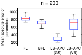
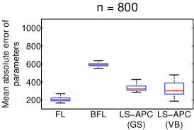
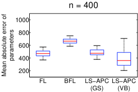
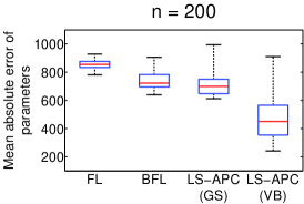
We first study the performance of the Fused lasso, Bayesian Fused lasso, and our LS-APC model (both the Gibbs sampler and Variational Bayes approximations) on two examples. All of them are based on the same linear model $y=X\beta+e$, where each entry in matrix $X$ was simulated from a univariate Gaussian distribution $X_{i,j}\sim\mathcal{N}\left(0,4\right)$ and vector $e$ follows multivariate Gaussian distribution $e\sim\mathcal{N}\left(\boldsymbol{0}_{n\times 1},200^{2}I_{n}\right)$. The ground truth vector of the regression coefficients was chosen to be both sparse and smooth, its length is $p=500$ and the number of nonzero coefficients is $70$. These coefficients form three blocks in the first example, two of these blocks have the shape of exponential growth and decrease, respectively, and one bell shaped (Gaussian-like) curve. In the second example, there is only one non-zero constant block, its length is $50$. The second shape was tested to verify the tendency of the fused lasso to choose piece-wise constant solutions. Both chosen shapes of regression coefficients are shown in Figure 1.

Figure 1: Simulated ground truth vector of regression coefficients $\beta$. Left: profile using exponential and bell shaped curves. Right: piecewise constant profile.

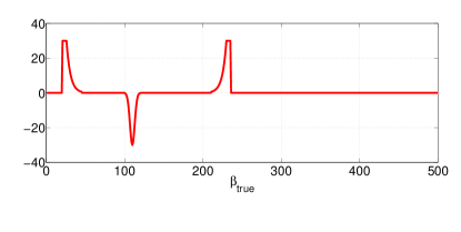
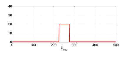
Performance of the compared methods was tested for different number of observation. In all cases, the optimal tuning coefficients for the fused lasso were found using 5 fold cross validation as implemented in HDPenReg R package, and the number of iterations for both BFL Gibbs sampler and our LS-APC Gibbs sampler algorithm was 50 000, where the first 5 000 samples were discarded as a burn in.

Evaluation of all simulation studies is done using absolute error, i.e. L1 distance of the resulting point estimates from the true parameter:

$$\text{AE}=\sum_{j=1}^{p}\left|\hat{\beta}_{j}-\beta_{j}^{true}\right|$$ (18)

The point estimate $\hat{\beta}$ is chosen to be the maximum of the posterior distribution. This is motivated by the results of the Gibbs samplers, which contain many outliers. The maximum is less sensitive to the realization of the sampler.

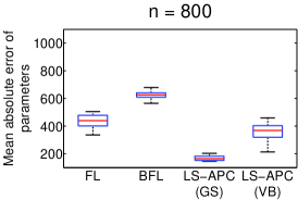
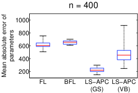
Results of Monte Carlo study of the tested methods for 20 realizations of the linear model with first shape of the parameter (exponentials and bell curve) is displayed in Figure 2 for $n\in\left[800,400,200\right]$ observations. Results of the same experiment for the second shape of the parameter (piecewise constant) are displayed in Figure 3. Indeed, with sufficient amount of observation, the Fused Lasso tuned by cross-validation outperformed all competing method for piece-wise constant parameter. However, with lower number observations and for more complex parameter shape, the Bayesian versions are outperforming it. The LS-APC variants systematically outperforming the BFL on all variants. As a mean field approximation, the VB methods is most sensitive to realization of the measurement error. However, its execution time is a fraction of all competing methods, therefore it may be a viable candidate for processing of large data. Note that even its worst performance is often comparable to that of the FL or BFL.

Figure 2: Comparison of L1 norm of error of parameter estimate for different number of observations $n$ of the simulated model with exponentials and bell curve, Figure 1 left. Compared methods are: Fused lasso (FL), Bayesian Fused lasso (BFL), and LS-APC model inferred by the Gibbs sampler (GS) and the Variational Bayes (VB) respectively.

Figure 3: Comparison of L1 norm of error of parameter estimate for different number of observations of the simulated model with piecewise constant, Figure 1 right. Compared methods are: Fused lasso (FL), Bayesian Fused lasso (BFL), and LS-APC model inferred by the Gibbs sampler (GS) and the Variational Bayes (VB) respectively.

5 The European Tracer Experiment Data

The motivation of our research is inversion modeling of atmospheric releases of aerosols Stohl et al. (2012), where the LS-APC model was successfully applied by Tichý et al. (2016). One of the best data sets in this field is the ETEX data. The European tracer experiment (ETEX) were two long time prepared experiments that took place in autumn 1994 in the north-western part of France. During both of them, 340 kg of perfluoromethylcyclohexane, breathable, well-traceable chemical, was released and its spread was tracked via a grid of 168 ground stations located in 17 European countries. The furthest station was more than 2000 km away from the source. An airborne measurement support was provided by 3 airplanes, but we did not include these observations.

During the first experiment, from which we have the data available, 340 kg of perflurocarbon was released in period of 12 hours, starting on 23 October, 16:00 UTC and ending at 04:00 UTC. At each ground station, automated sequential air samplers operated sampling every 3 hours for a total period of 72 hours. These samples are arranged in vector $y$ of length $3102$. We consider the task of estimation of the temporal profile of the source activity from the known location. The common methodology is based on running a simulation model with unit release for each hour in the potential release time window. Since the chemical is not reactive, the measured concentration is a superposition of contributions from each hour of the release weighted by the released amount of the tracer in that hour. The observations are thus explained by a linear model with regression coefficients given by numerical simulation model.

5.1 Construction of the Regressor Matrix

We have used version 8.1 of the Lagrangian particle dispersion model FLEXPART Stohl et al. (1998) for construction of the matrix of regressors $X$. This matrix is known as the source-receptor sensitivity matrix in the atmospheric science. We used the same setup as Tichý et al. (2016); Martinez-Camara et al. (2014) simulating a series of 1hour releases for the period of 5 days containing the true release. The length of the unknown release profile $\beta$ is thus 120. The model was driven by 40-year re-analysis meteorelogical data (ERA-40) using model time step in the boundary layer limited to less than 20% of the Lagrangian timescale and a maximum value of 300 s. The simulation was evaluated for all sensors in the observation network.

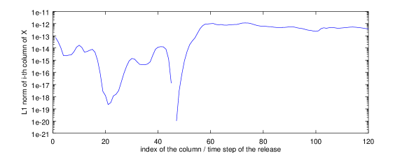
The regressor matrix $X$ is poorly conditioned as demonstrated in Figure 4 via L1 norm of its columns. Note that in time step 46, the sum of the regressors is exactly zero. Therefore, any value of $x_{46}$ will contribute zero to the measurements. Sensitivity of the measurements to parameter values with indeces lower than 54 is also very low. Therefore, we will study behavior of the methods also for 66 hours with time index $54$ to $120$, this reduced dataset will be denoted as ETEX 66.

Figure 4: Visualization of matrix $X$ via logarithm of the L1 norm of its columns.

5.2 Covariance Matrix of the Observations

Since the matrix $X$ is computed from estimated meteorological data, it may be subject to a systematic error. Thus, the observation error may not be independent. For example, if the estimated wind speed is different from the true wind speed, the model residues would be correlated in time. Since we can not estimate the full matrix of observations, we define a finite set of covariance matrices of the observation noise and use them as models in the model selection procedure.

Specifically, we consider the noise to be Gaussian $e\sim\mathcal{N}\left(\boldsymbol{0}_{n\times 1},\sigma^{-1}B^{-1}\right)$, with

$$B_{i,j}=\begin{cases}1&\text{if }i=j,\\ \xi&\text{site}\left(i\right)=\text{site}\left(j\right)\\ 0&\text{otherwise}.\end{cases}\text{ and }|\text{time}\left(i\right)-\text{time}\left(j\right)|=3\text{hours},$$ (19)

Hyperparameter $\xi$ is used to model correlation between every two measurements of the same ground station that are taken in the subsequent time samples (i.e. 3 hours). The value of $\xi$ also influences positive definiteness of matrix $B^{-1}$ restricting its possible values. We have selected a finite grid of $\xi$ and for each value we perform data transformation

$$\tilde{y}_{k} =\text{chol}\left(B\left(\xi_{k}\right)\right)^{-1}y, \tilde{X}_{k} =\text{chol}\left(B\left(\xi_{k}\right)\right)^{-1}X,\,\,k=1,\ldots,m.$$ (20)

Under the assumption that the model is correct, the transformed data satisfy model (6). Note that the conventional uncorrelated noise is a special case of (19) for $\xi=0$.

Remark: We have defined a much larger set of covariance matrices considering correlation of locations (which could be caused e.g. by error in the wind direction), or weighting by distance of the receptors. None of these models was found to be significant. Therefore, we report only results of the time-correlated observation covariance.

5.3 Positivity Enforcement

Another important feature of the ETEX data is that the released amount of the tracer can not be negative. Thus the support of the prior on $\beta$ is constrained to positive real numbers. The prior of $\beta$ is then a truncated multivariate Gaussian distribution. This influences evaluation of the posterior in both estimation techniques. Specifically, in the Variational Bayes approach, the shaping distributions are identical to those with unconstrained version, however, the moments are evaluated with respect to the truncated region Tichý et al. (2016).

The Gibbs sampler requires to sample from the multivariate truncated Gaussian distribution. We have used algorithm of Li and Ghosh (2015) for this purpose.

5.4 Model Selection

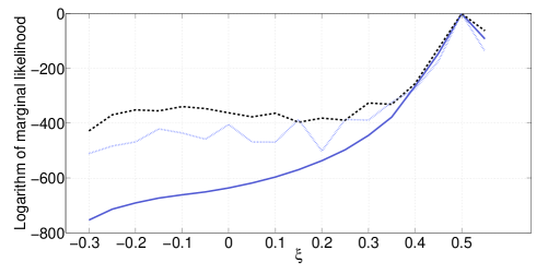
Different transformations of the data (20) allow us to compare performance of both tested inference methods for model selection of the LS-APC model: the Variational Bayes and the Gibbs sampler. Since the marginal likelihood values were extremely low, we report the logarithm of the marginal likelihood relative to its maximum value for each method in Table 1 and Figure 5. For comparison, we also evaluated the Gibbs sampling for two choices of $\theta^{*}$: the maximum aposteriori estimate and the median estimate. Note that all inference methods decisively select the model with $\xi=0.45$ as the most likely model.

The correspondence of the model likelihood from the Variational Bayes method with that of the Gibbs sampler is remarkably good. The Variational Bayes tends to underestimate the variance of the estimate (Bishop (2006a)), which may be the reason why the marginal log-likelihood is underestimated for the less likely models.

$\xi$	-0.2	-0.1	0	0.1	0.2	0.3	0.35	0.4	0.45	0.5
GS med.	-421	-459	-469	-387	-386	-323	-275	-174	0	-137
GS MAP	-355	-347	-377	-396	-389	-331	-256	-128	0	-62
VB	-673	-651	-618	-570	-497	-378	-265	-146	0	-92

Table 1: Comparison of marginal log-likelihood of the LS-APC model for varying value of $\xi$.

Figure 5: Comparison of marginal log-likelihood of the LS-APC model for varying value of $\xi$. Dashed line denotes values obtained by Gibbs sampler with maximum posterior values as $\theta^{*}$ in (11) and dotted line denotes the same estimate using median as $\theta^{*}$. Full line denotes the results of the Variational Bayes method.

5.5 Estimated Source Term Profiles

In this Section, we provide results of estimation of the release profile for the ETEX data using all tested algorithms for error covariance model (19) with $\xi=0.45$.

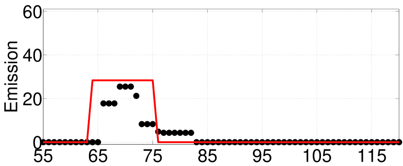
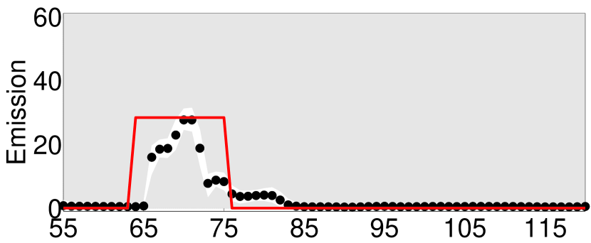
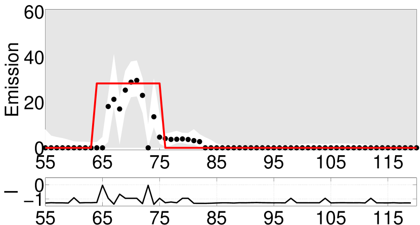
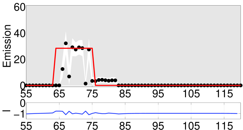
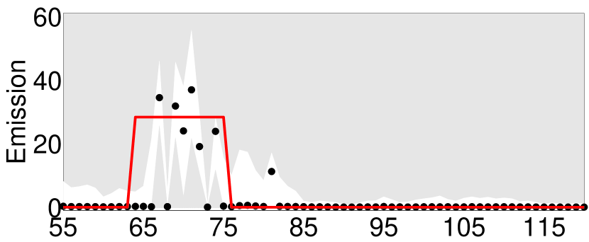
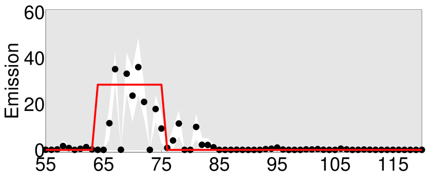
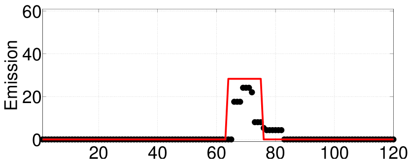
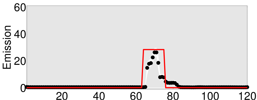
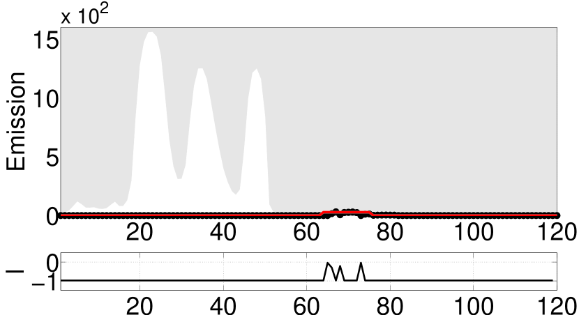
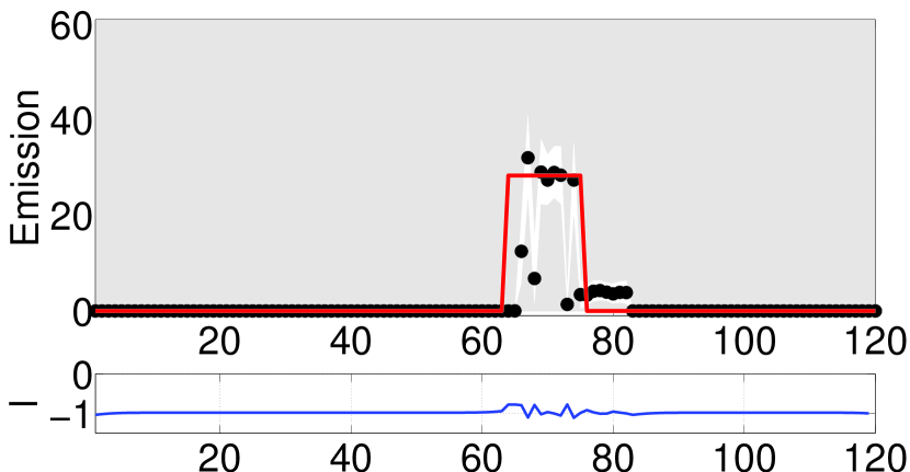
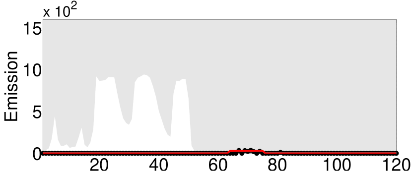
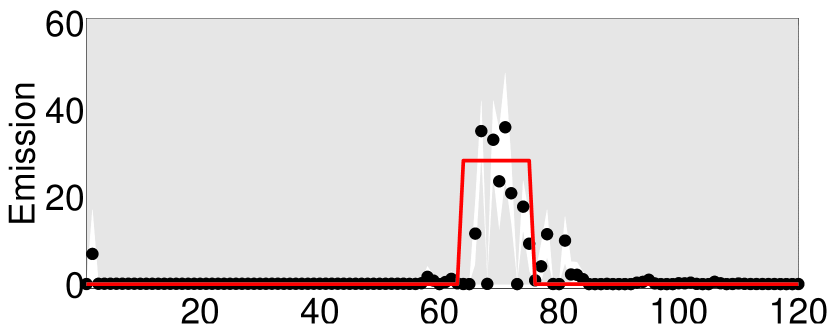
The resulting posterior distribution for the release profile are displayed in Figure 7 for the full ETEX data and in Figure 6 for the ETEX 66. The reason is that the 95% quantile of the release profile is very wide at time indexes with extremely low sensitivity of the measurements to the parameter as indicated in Figure 4. The estimates at the time of the true release are almost identical for both data sets as indicated by values of the absolute error of the MAP estimate.

Note that all methods provide acceptable results given how uncertain is the regressor matrix. It is impossible to draw definite conclusion from comparison of the the posterior estimates with the true release. Therefore, we will comment only on the qualitative indicators.

First, we focus on description of the period of informative data which is at the time of the true release. Note that the estimates of the release provided by the Fused Lasso and Bayesian Fused Lasso are very smooth with characteristic piece-wise constant shape. The uncertainty of the estimation in the BLF is lower compared to that of the LS-APC (GS) algorithm. On the other hand, the LS-APC algorithm enforces smoothness only mildly, as demonstrated in comparison with results of the same method with sparsity prior only (1) which corresponds to LS-AC with $l=0$. Results of the VB and GS approximations of the LS-APC model are well comparable, with VB providing narrower uncertainty bounds.

	FL	BFL	LS-APC	LS-APC	LS-APC	LS-APC
			(GS)	(VB)	(GS) $l=0$	(VB) $l=0$
ETEX	199.95	233.80	181.49	180.85	231.19	230.48
ETEX 66	194.94	215.98	186.52	180.85	224.34	231.34

Table 2: Absolute error of the MAP estimate of the release profile from the true release profile of the ETEX experiment.

Fused lasso	Bayesian Fused lasso
LS-APC (GS)	LS-APC (VB)
LS-APC (GS) without smoothness	LS-APC (VB) without smoothness

Figure 6: Posterior distribution of the release profile for the ETEX 66 data set via its maximum and 95% quantile. In all pictures, the red line marks the ground truth for $\beta$, black circles are the MAP estimate of $\beta$ and white area is the 95% quantile. The results of LS-APC method are accompanied by estimate of the correlation parameter $l$ in the lower plot.

Fused lasso	Bayesian Fused lasso
LS-APC (GS)	LS-APC (VB)
LS-APC (GS) without smoothness $l=0$	LS-APC (VB) without smoothness $l=0$

Figure 7: Posterior distribution of the release profile for the ETEX data set via its maximum and 95% quantile. In all pictures, the red line marks the ground truth for $\beta$, black circles are the MAP estimate of $\beta$ and white area is the 95% quantile. The results of LS-APC method are accompanied by estimate of the correlation parameter $l$ in the lower plot.

However, the difference in uncertainty handling between the GS and VB approximations is most visible at the period of uninformative data which is for time index less than 55. In this period, the 95% uncertainty interval for the GS algorithm is extremely wide while for the VB approximation, the posterior density is concentrated around zero. This is perhaps the most interesting feature LS-APC (GS) method. Due to low sensitivity of the measurements to the parameter values in this region, we can not reliably conclude that the tracer was not being released at this time. The LS-APC(GS) algorithms thus provides the most conservative answer which is desirable in this application domain.

6 Conclusion

We have analyzed two prior models encouraging smoothness and sparsity of the linear regression model, the Bayesian Fused Lasso and the Least Squares with adaptive prior covariance matrix. The derived Gibbs sampling algorithm for the latter was found to provide the best results on simulated and real data from the European tracer experiment. However, even the original Variational Bayes inference of the LS-APC model was found to be well suitable for large data set arising in atmospheric science due to its computational speed. The drawback of the variational method is underestimation of the uncertainty of the estimate. However, the variational lower bound for the marginal likelihood (i.e. Bayes factor for the model selection problem) was found to be in very good agreement with the same value provided by the Gibbs sampling.

Since the LS-APC method allows to define an arbitrary conditionally independent structure of the covariance matrix, the method can be readily used in wide range of applications.

References

- Alhamzawi et al. (2012) Alhamzawi, R., Yu, K., and Benoit, D. F. (2012). Bayesian adaptive lasso quantile regression. Statistical Modelling, 12(3), 279–297.
- Bien et al. (2013) Bien, J., Taylor, J., and Tibshirani, R. (2013). A lasso for hierarchical interactions. Annals of statistics, 41(3).
- Bishop (2006a) Bishop, C. (2006a). Pattern recognition and machine learning, volume 1. springer New York.
- Bishop (2006b) Bishop, C. M. (2006b). Pattern Recognition and Machine Learning. Springer.
- Cai et al. (2012) Cai, B., Lawson, A. B., Hossain, M. M., and Choi, J. (2012). Bayesian latent structure models with space-time dependent covariates. Statistical modelling, 12(2), 145–164.
- Chantas et al. (2010) Chantas, G., Galatsanos, N. P., Molina, R., and Katsaggelos, A. K. (2010). Variational bayesian image restoration with a product of spatially weighted total variation image priors. IEEE transactions on image processing, 19(2), 351–362.
- Chib (1995) Chib, S. (1995). Marginal likelihood from the gibbs output. Journal of the American Statistical Association, 90(432), 1313–1321.
- Eckhardt et al. (2008) Eckhardt, S., Prata, A., Seibert, P., Stebel, K., and Stohl, A. (2008). Estimation of the vertical profile of sulfur dioxide injection into the atmosphere by a volcanic eruption using satellite column measurements and inverse transport modeling. Atmospheric Chemistry and Physics, 8(14), 3881–3897.
- Friedman et al. (2008) Friedman, J., Hastie, T., and Tibshirani, R. (2008). Sparse inverse covariance estimation with the graphical lasso. Biostatistics, 9(3), 432–441.
- Ganesan et al. (2014) Ganesan, A., Rigby, M., Zammit-Mangion, A., Manning, A., Prinn, R., Fraser, P., Harth, C., Kim, K.-R., Krummel, P., and Li, S. (2014). Characterization of uncertainties in atmospheric trace gas inversions using hierarchical Bayesian methods. Atmospheric Chemistry and Physics, 14(8), 3855–3864.
- George and McCulloch (1993) George, E. I. and McCulloch, R. E. (1993). Variable selection via Gibbs sampling. Journal of the American Statistical Association, 88(423), 881–889.
- Grimonprez and Iovleff (2016) Grimonprez, Q. and Iovleff, S. (2016). HDPenReg: High-Dimensional Penalized Regression. URL https://CRAN.R-project.org/package=HDPenReg. R package version 0.93.1.
- Henne et al. (2016) Henne, S., Brunner, D., Oney, B., Leuenberger, M., Eugster, W., Bamberger, I., Meinhardt, F., Steinbacher, M., and Emmenegger, L. (2016). Validation of the Swiss methane emission inventory by atmospheric observations and inverse modelling. Atmospheric Chemistry and Physics, 16(6), 3683–3710.
- Kyung et al. (2010) Kyung, M., Gill, J., Ghosh, M., Casella, G., et al. (2010). Penalized regression, standard errors, and bayesian lassos. Bayesian Analysis, 5(2), 369–411.
- Li and Ghosh (2015) Li, Y. and Ghosh, S. (2015). Variables sampling mmethod for truncated multivariate normal and student distributions subject to linear inequality constraints. Journal of Statistical Theory and Practice, 9(4), 712–732.
- Martinez-Camara et al. (2014) Martinez-Camara, M., Béjar Haro, B., Stohl, A., and Vetterli, M. (2014). A robust method for inverse transport modeling of atmospheric emissions using blind outlier detection. Geoscientific Model Development, 7(5), 2303–2311.
- Meier et al. (2008) Meier, L., Van De Geer, S., and Bühlmann, P. (2008). The group lasso for logistic regression. Journal of the Royal Statistical Society: Series B (Statistical Methodology), 70(1), 53–71.
- Miazhynskaia and Dorffner (2006) Miazhynskaia, T. and Dorffner, G. (2006). A comparison of bayesian model selection based on mcmc with an application to garch-type models. Statistical Papers, 47(4), 525–549.
- Ormerod and Wand (2010) Ormerod, J. T. and Wand, M. P. (2010). Explaining variational approximations. The American Statistician, 64(2), 140–153.
- Park and Casella (2008) Park, T. and Casella, G. (2008). The bayesian lasso. Journal of the American Statistical Association, 103(482), 681–686.
- Perrakis et al. (2014) Perrakis, K., Ntzoufras, I., and Tsionas, E. G. (2014). On the use of marginal posteriors in marginal likelihood estimation via importance sampling. Computational Statistics & Data Analysis, 77, 54–69.
- Ročková and George (2015) Ročková, V. and George, E. (2015). The spike-and-slab lasso. Journal of the American Statistical Association, Theory and Methods. in review.
- Stohl et al. (2012) Stohl, A., Seibert, P., Wotawa, G., Arnold, D., Burkhart, J., Eckhardt, S., Tapia, C., Vargas, A., and Yasunari, T. (2012). Xenon-133 and Caesium-137 releases into the atmosphere from the Fukushima Dai-ichi nuclear power plant: determination of the source term, atmospheric dispersion, and deposition. Atmospheric Chemistry and Physics, 12(5), 2313–2343.
- Stohl et al. (1998) Stohl, A., Hittenberger, M., and Wotawa, G. (1998). Validation of the lagrangian particle dispersion model flexpart against large-scale tracer experiment data. Atmospheric Environment, 32(24), 4245–4264.
- Tibshirani (1996) Tibshirani, R. (1996). Regression shrinkage and selection via the lasso. Journal of the Royal Statistical Society, 58(1), 267–288.
- Tibshirani et al. (2005a) Tibshirani, R., Saunders, M., Rosset, S., Zhu, J., and Knight, K. (2005a). Sparsity and smoothness via the fused lasso. Journal of the Royal Statistical Society: Series B (Statistical Methodology), 67(1), 91–108.
- Tibshirani et al. (2005b) Tibshirani, R., Saunders, M., Rosset, S., Zhu, J., and Knight, K. (2005b). Sparsity and smoothness via the fused lasso. Journal of the Royal Statistical Society: Series B (Statistical Methodology), 67(1), 91–108.
- Tichý et al. (2016) Tichý, O., Šmídl, V., Hofman, R., and Stohl, A. (2016). LS-APC v1.0: a tuning-free method for the linear inverse problem and its application to source-term determination. Geoscientific Model Development, 9(11), 4297–4311.
- Tipping (2001) Tipping, M. (2001). Sparse Bayesian learning and the relevance vector machine. The journal of machine learning research, 1, 211–244.
- Šmídl and Quinn (2006) Šmídl, V. and Quinn, A. (2006). The Variational Bayes Method in Signal Processing. Springer.
- Xu and Ghosh (2015) Xu, X. and Ghosh, M. (2015). Bayesian variable selection and estimation for group lasso. Bayesian Analysis, 10(4), 909–936.