The first study of the Light-Travel Time Effect in bright eclipsing binaries in the Small Magellanic Cloud

Abstract

The first 100 brightest eclipsing systems from the Small Magellanic Cloud (SMC) were studied for their period changes. The photometric data from the surveys OGLE-II, OGLE-III, OGLE-IV, and MACHO were combined with our new CCD observations obtained using the Danish 1.54-meter telescope (La Silla, Chile). Besides the period changes also the light curves were analysed using the program PHOEBE, which provided the physical parameters of both eclipsing components. For fourteen of these systems the additional bodies were found, having the orbital periods from 2 to 20  years and the eccentricities were found to be up to 0.9. Among the sample of studied 100 brightest systems we discussed the number of systems with particular period changes. About 10% of these stars show eccentric orbit, about the same number have third bodies and about the same show the asymmetric light curves.

1 Introduction

The classical eclipsing binaries still play a crucial role in modern astrophysics. We can study the eclipsing binary (hereafter EB) light curve, and model its shape, revealing the physical parameters of both eclipsing components as well as their mutual orbit (see e.g. Kallrath & Milone 2009). It is still the most precise method to derive the individual masses, radii, and luminosities of components (see e.g. Southworth 2012).

The same apply also for the role of the EBs outside of our Milky Way Galaxy, however obtaining good observations is much more tricky and time-consuming due to their low brightness. Hence, we usually deal with a lack of data for analysis. This aspect has changed rapidly during the last two decades thanks to the large photometric surveys like OGLE and MACHO. Owing to the long-lasting photometric monitoring of the Magellanic Clouds (OGLE II, III and IV cover 16 seasons), almost 50000 EBs are known outside our Galaxy (Pawlak et al., 2016), and many of them are interesting enough for further more detailed analysis. Hence, here comes our contribution to the topic.

As a well-known fact, the Magellanic Clouds have slightly different metallicity than our Milky Way Galaxy (see e.g. Westerlund 1997, or Davies et al. 2015). Therefore, we can study whether this effect plays a role in eclipsing binary research, whether it is traceable in the models, or whether our data are sufficiently precise to distinguish between models with different metallicities. We can also study the stellar multiplicity in general – Is the frequency of multiple systems the same in Magellanic Clouds as in our own Galaxy? Borkovits et al. (2016) show quite recently that of about 1/12 of all eclipsing binaries observed by the Kepler space telescope probably contain additional components that can be detected only via eclipse timing variations. Is this number roughly the same in other stellar sample, even outside Milky Way?

2 The system selection

Continuing our similar study of period changes in eight eclipsing binaries located in LMC (Zasche et al., 2016), we now moved our attention to the SMC galaxy and another approach. Due to the well-known fact that the probability of detecting another third component in eclipsing binary strongly depends on the primary mass (see e.g. Duchêne & Kraus 2013), we focused on the most massive stars (hence also the most luminous ones from the OGLE survey). Therefore, we took the first one hundred brightest targets in the OGLE III survey from the SMC galaxy (more precisely: in the $I$ filter) and performed the analysis of its period changes. Additionally, some targets were also added to this sample as by-chance discoveries in some of our monitored fields.

The selection criterion based on the data quality was as follows. We have chosen only such systems, which have the depths of their minima deeper than the scatter of the light curve itself

Another selection criterion was the data coverage. Because we focused on periodic variations in the $O-C$ diagrams, we decided to include in our study those systems, which have at least one period of the variation already covered (either with the survey data or our own observations).

3 The analysis

The method was the same as in our previous paper (Zasche et al., 2016), which means that the whole time interval was divided into several seasons and the light curve template from the PHOEBE (see below) fit was used for deriving the individual times of minima. If there was some obvious change of its orbital period, then the system was classified as a suspicious and analysed in more detail. This means that also the other available photometry was collected, mostly the Macho (Faccioli et al., 2007), OGLE II (Wyrzykowski et al., 2004), and OGLE III (Pawlak et al., 2013), and OGLE IV (Pawlak et al., 2016) databases. Moreover, for some of the systems we also collected some new data using the Danish 1.54-meter telescope located at the La Silla Observatory in Chile. The data mining from all these data sources together with our new photometry led to the selection of fourteen interesting systems showing periodic modulation of their orbital periods.

The light curve (hereafter LC) analysis was carried out using the program PHOEBE (Prša & Zwitter, 2005), based on the Wilson-Devinney algorithm (Wilson & Devinney, 1971) and its later modifications. We used the OGLE III data for the light curve modelling, because these are typically of the best quality, obtained over the longer time span and the phase light curves are well-covered.

The PHOEBE code enables us to construct the theoretical LC, which is later used as a template to derive the times of eclipses. Hence, our LC fit needs to be as precise as possible. For all of our fourteen system we found that their orbits are circular, hence the eccentricity was fixed at zero. For the starting ephemerides, we used the same ones as published by Pawlak et al. (2013) in their catalogue and later modified according to the period changes. The primary temperatures were derived from the published photometric indices by Massey (2002), and Zaritsky et al. (2002). For only a few systems their spectral types or primary temperatures were published, then we used these values, of course. See Table 1 for more information about the individual systems in our sample.

Therefore, the set of the fitted quantities was the following: The temperature of the secondary component $T_{2}$, the inclination angle $i$, the Kopal’s modified potentials $\Omega_{i}$, and the luminosities of the components $L_{i}$. Having no information about the radial velocities, the mass ratio can only hardly be derived (see e.g. Terrell & Wilson 2005), hence we fixed it to $q=1.0$. The limb darkening coefficients were interpolated from the van Hamme s tables (van Hamme, 1993), and the synchronicity parameters ($F_{i}$) were also kept fixed at values of $F_{i}=1$. Because we deal with very hot stars here, we also fixed the albedo coefficients $A_{i}$ at a value 1.0, as well as the gravity darkening coefficients $g_{i}=1.0$.

For studying the apparent variations of the orbital period in these binaries, we used a well-known "Light-Travel Time Effect" (or LTTE) hypothesis (Irwin, 1959). It is based on the assumption that the two eclipsing stars are being accompanied by some hidden distant component, orbiting around the common barycenter with the eclipsing pair. Hence, we deal with a classical hierarchical system. As the pair moves around a common center of mass, the eclipses of the binary occur earlier or later depending on the current position of the stars with respect to the observer. For some discussion and limitations of this method see for instance Mayer (1990). A similar method was used quite recently for discovering several dozens of new triple systems in the Kepler field, see Borkovits et al. (2016) or Gies et al. (2015). As far as we know, there was no other study analysing the period changes via LTTE located in the SMC published until yet, only the paper studying the 90 systems with apsidal motion by Hong et al. (2016).

The times of minima for the analysed systems were derived using the AFP method presented in Zasche et al. (2014). This method uses the LC template as derived from the PHOEBE and shifts the template in both $x$ and $y$ axes together with the phased light curve in the particular dataset to achieve the best fit. These datasets were constructed according to the quality and density of the data (for the OGLE this usually means one dataset per one year of observations, but for short-periodic variables more fine division into datasets was used). Using the MACHO, OGLE and our new data we obtained minima times spanning over many years. Hence, detecting the orbital periods of the order of a few years to a decade was possible.

The whole fitting process was performed in several steps. At first the ephemerides from Pawlak et al. (2013) were used and the preliminary solution was found in PHOEBE (using typically one season of OGLE data with the best coverage). With this light curve template the AFP method produced some preliminary minima times and we were able to see whether the system was suitable for a further analysis or not. The second step was the $O-C$ analysis, refining the orbital period which was then used in PHOEBE for a more detailed modelling of the light curve. With the final light curve template the final times of minima were derived and the $O-C$ analysis was performed. Different kinds of modulations of the orbital period can be studied in this way, but we focused only on the periodic modulation. Sometimes our approach only led to improvement of the linear ephemerides and no variation was found. Sometimes, some other phenomena were found, but such systems are not of our interest and these systems are only briefly summarized below in Section 5.

However, at this place we have to emphasize that the solutions presented are only mathematical ones, and especially the errors (e.g. from PHOEBE) can sometimes be rather underestimated. More discussion about the conclusiveness of the fits are given below in Section 6.

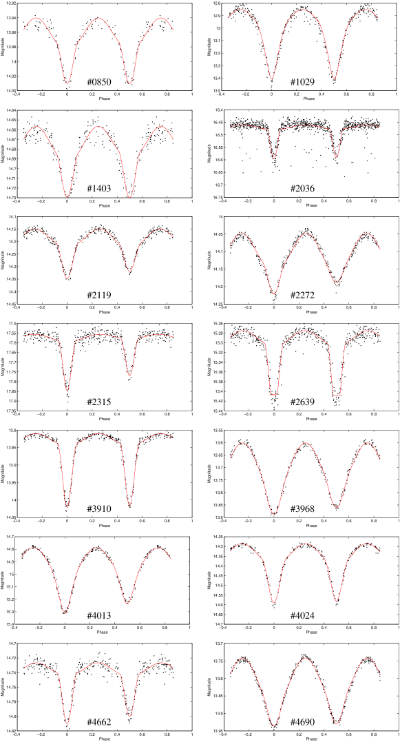
Figure 1: Plot of the light curves of the analysed systems.

4 Individual systems

For all of the tables and pictures below we decided to use an abbreviation of the long OGLE III names. Therefore, instead of, for instance, OGLE-SMC-ECL-0850, we use only the $\#$0850 for a better clarity.

Because the method of analysis is the same for all of the studied systems and the results are sometimes similar, we focus only on the most interesting ones in our sample and discuss them in more detail in the following subsections. The results are summarized in Tables 1, 2, and 3, while the final plots are given in Figures 1, and 2.

4.1 OGLE-SMC-ECL-1403

The system OGLE-SMC-ECL-1403 was found to be the detached one, with both rather hot components. Quite surprising was high mass function of the predicted third body $f(m_{3})$, which resulted from rather short period $p_{3}$. However, even such solution is plausible, because also very high level of the third light in the LC solution $L_{3}$ was found.

4.2 OGLE-SMC-ECL-2036

A similar situation is also for the system OGLE-SMC-ECL-2036, where a high value of the mass function $f(m_{3})$ is substantiated by the very high level of the third light from the LC solution. The obvious high scatter of the LC is caused by difficult reduction due to the close bright stars.

4.3 OGLE-SMC-ECL-2119

The system OGLE-SMC-ECL-2119 is one of a few already analysed and published systems. Hilditch et al. (2005) collected besides the photometry also 17 spectra, and the analysis yielded that both eclipsing components are of O9 spectral type, with the mass ratio of 1.086. This value was also kept fixed during our LC fitting, together with the fixed $T_{1}$ temperature. There resulted that the third light is significant, but not dominant (the previous study was not taking the $L_{3}$ contribution as a free parameter). Our solution of the period changes resulted in a consistent figure with a significant third body on a 5-yr orbit.

4.4 OGLE-SMC-ECL-2272

This was the only system in our sample, which shows a small asymmetry of its LC, where primary and secondary minima appear slightly shifted from their positions in 0.0 and 0.5 in phase. In detached configuration this usually means that the system is eccentric, however here we deal with a semidetached configuration, hence this explanation is odd. As was shown elsewhere (e.g. Zasche 2011) the asymmetric light curves sometimes mimic the false eccentricity also in contact binaries. Hence, we shifted both primary and secondary minima to one common ephemerides and performed the period analysis. This approach is justified due to the fact that both primary and secondary minima behave in the same way and the periodic modulation with the period of about 7.6 yr is clearly seen in both of them.

4.5 OGLE-SMC-ECL-3910

Another case where at least some information can be found in the already published papers, see Massey et al. (2012). The authors provided information about the spectral types of the components to be of O5+O7 with a very important remark that there are some triple lines visible in the spectra, which are also shifting. Hence, our analysis of the LC together with the period changes clearly confirms their finding.

4.6 OGLE-SMC-ECL-3968

The system with the shortest detected period of the LTTE of about 2 years, and also with the second shortest period of the inner eclipsing pair.

4.7 OGLE-SMC-ECL-4013

In this case there was quite problematic calibration of the temperature $T_{1}$ due to the ill-defined value of the photometric index $(B-V)_{0}$. Therefore, we simply fixed the $T_{1}$ to 10000 K.

4.8 OGLE-SMC-ECL-4024

The system OGLE-SMC-ECL-4024 was found to exhibit double periodic modulation in its $O-C$ diagram. Hence, we used the LTTE hypothesis two times for a detailed description of the minima times observations. The results are plotted in Fig. 2, where both modulations are clearly visible. Pure LTTE combined with the quadratic ephemerides are not able to describe the data in detail. Parameters of both LTTE variations are given on separate lines in Table 3. Such systems were seldom discovered in our Galaxy, but this is the first time any such system is being detected outside of Galaxy.

4.9 OGLE-SMC-ECL-4690

The last system in our set of stars also seems to be slightly asymmetric, a similar situation as for $\#$2272. But here we ignored this asymmetry, which yielded to the $O-C$ diagram in Fig. 2, where the primary and secondary minima are slightly shifted, but both follow similar period variation.

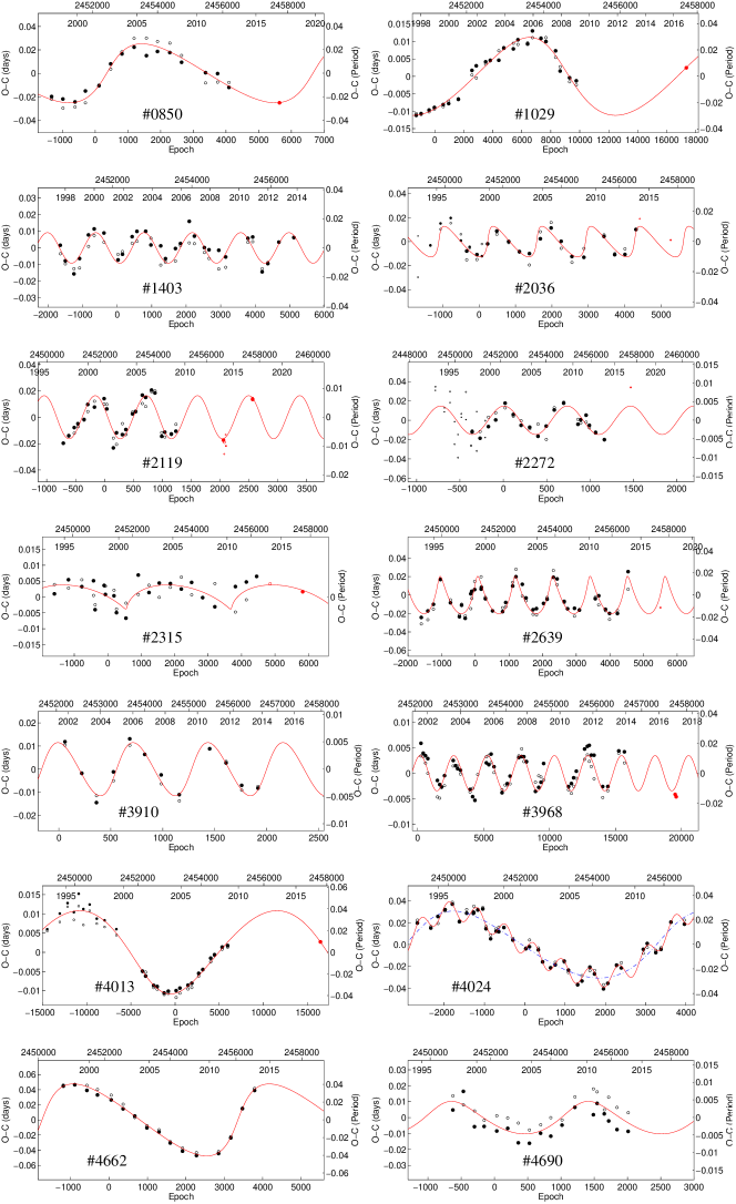
Figure 2: Plot of the $O-C$ diagrams of the analysed systems. The solid lines represent the final LTTE fit, filled points stand for the primary minima, while the open circles for the secondary ones, bigger the symbol, better the precision. The red data points represent our new observations.

Table 1: Identification of the analysed systems.

System	OGLE II 1	MACHO	RA	DE	$I_{\rm max}^{\,2}$	$(V-I)^{\,3}$	$(B-V)_{0}^{\,4}$
OGLE-SMC-ECL-0850	SC3 202715		00h45m18s.20	-73∘15′23${}^{\prime\prime}\!$.1	13.936	-0.167	-0.314
OGLE-SMC-ECL-1029	SC4 88435		00h46m19s.67	-72∘50′56${}^{\prime\prime}\!$.7	12.858	0.796	-0.009
OGLE-SMC-ECL-1403	SC4 175130		00h48m17s.96	-73∘07′19${}^{\prime\prime}\!$.0	14.658	-0.124	-0.282
OGLE-SMC-ECL-2036	SC5 306002	208.16026.98	00h51m04s.28	-72∘47′38${}^{\prime\prime}\!$.9	16.463	-0.075	-0.144
OGLE-SMC-ECL-2119	SC5 305884		00h51m20s.18	-72∘49′43${}^{\prime\prime}\!$.4	14.150	-0.147	-0.268
OGLE-SMC-ECL-2272	SC6 77224	208.16085.16	00h51m50s.13	-72∘39′23${}^{\prime\prime}\!$.1	14.048	-0.151	-0.285
OGLE-SMC-ECL-2315	SC6 67920	208.16084.320	00h52m01s.16	-72∘44′41${}^{\prime\prime}\!$.8	17.572	-0.073	-0.105
OGLE-SMC-ECL-2639	SC6 232226	207.16140.25	00h53m07s.01	-72∘46′21${}^{\prime\prime}\!$.0	15.289	-0.159	-0.290
OGLE-SMC-ECL-3910			00h59m00s.04	-72∘10′38${}^{\prime\prime}\!$.1	13.825		-0.322
OGLE-SMC-ECL-3968			00h59m20s.47	-71∘21′42${}^{\prime\prime}\!$.4	13.616		-0.018
OGLE-SMC-ECL-4013		211.16529.5	00h59m31s.20	-73∘26′56${}^{\prime\prime}\!$.0	14.782		-0.358
OGLE-SMC-ECL-4024	SC8 129157	211.16539.2	00h59m34s.19	-72∘46′57${}^{\prime\prime}\!$.9	14.292	-0.218	-0.278
OGLE-SMC-ECL-4662	SC9 163573		01h03m13s.97	-72∘25′07${}^{\prime\prime}\!$.6	14.737	-0.214	-0.323
OGLE-SMC-ECL-4690	SC9 175323		01h03m21s.30	-72∘05′38${}^{\prime\prime}\!$.2	13.740	-0.183	-0.313

Notes: [1] - The full name from the OGLE II survey should be OGLE LMC-SCn nnnnnn, [2] - Value taken from Pawlak et al. (2013), [3] - Value taken from Udalski et al. (1998), [4] Dereddened value derived from the (B-V) and (U-B) indices taken from Massey (2002) or Zaritsky et al. (2002).

Table 2: Light curve parameters for the analysed systems, the results from PHOEBE.

System	$T_{1}$ (fixed)	$T_{2}$	Type 1	$i$ [deg]	$\Omega_{1}$	$\Omega_{2}$	$L_{1}$ [%]	$L_{2}$ [%]	$L_{3}$ [%]
$\#$0850	32000	28222 (450)	D	60.44 (0.76)	4.160 (0.040)	4.265 (0.039)	50.4 (1.9)	36.9 (0.7)	12.7 (1.2)
$\#$1029	9700	10183 (95)	OC	78.19 (0.59)	3.692 (0.019)	–	47.3 (0.7)	51.5 (0.8)	1.2 (1.0)
$\#$1403	25000	24743 (651)	D	62.58 (1.08)	3.898 (0.057)	4.236 (0.095)	22.9 (1.3)	17.4 (2.1)	59.7 (3.2)
$\#$2036	15000	14406 (420)	D	85.04 (0.85)	5.341 (0.139)	6.035 (0.210)	16.9 (0.9)	11.6 (0.7)	71.5 (9.7)
$\#$2119	33800	31227 (368)	D	67.14 (0.55)	4.962 (0.082)	3.964 (0.015)	27.6 (0.7)	53.8 (1.4)	18.6 (2.6)
$\#$2272	29000	24948 (337)	SD	60.09 (0.68)	3.943 (0.052)	–	38.0 (1.7)	33.8 (1.1)	28.2 (1.7)
$\#$2315	16000	13071 (245)	D	76.24 (0.76)	5.015 (0.098)	5.245 (0.085)	55.2 (1.1)	36.4 (2.3)	8.4 (1.9)
$\#$2639	26000	25920 (312)	D	84.57 (0.89)	4.146 (0.049)	6.431 (0.088)	30.3 (4.4)	9.5 (2.0)	60.2 (6.7)
$\#$3910	41000	40218 (489)	D	72.54 (0.35)	4.759 (0.041)	4.923 (0.024)	50.9 (1.2)	44.7 (0.9)	4.4 (0.9)
$\#$3968	10000	9241 (101)	SD	62.08 (0.19)	3.713 (0.015)	–	53.3 (0.9)	46.7 (1.2)	0.0
$\#$4013	10000	8839 (74)	OC	73.33 (0.51)	3.708 (0.030)	–	55.2 (0.7)	44.8 (0.7)	0.0
$\#$4024	26000	25697 (345)	D	85.15 (1.08)	3.754 (0.049)	3.921 (0.055)	26.7 (2.1)	22.6 (0.9)	50.6 (1.7)
$\#$4662	33000	30078 (389)	D	66.92 (1.01)	4.438 (0.051)	4.747 (0.061)	35.1 (2.0)	23.9 (2.3)	41.0 (4.2)
$\#$4690	41000	39034 (392)	OC	58.44 (0.49)	3.129 (0.027)	–	50.5 (2.3)	31.1 (0.8)	18.4 (3.4)

Notes: [1] - D=Detached, OC=Overcontact, SD=Semidetached,

Table 3: The parameters of the third-body orbits for the individual systems.

System	$HJD_{0}$	$P$	$A$	$\omega$	$P_{3}$	$T_{0}$ [HJD]	e	$f(m_{3})$	$P_{3}^{2}/P$
	(2450000+)	[days]	[days]	[deg]	[yr]	(2400000+)		$[M_{\odot}]$	[yr]
$\#$0850	2088.833 (4)	1.0028183 (12)	0.0252 (28)	4.0 (12.1)	17.3 (3.2)	84108 (925)	0.465 (24)	0.398 (21)	109223
$\#$1029	1176.969 (2)	0.3766298 (3)	0.0111 (4)	156.5 (17.0)	14.4 (0.6)	54399 (204)	0.264 (59)	0.038 (1)	200598
$\#$1403	2121.714 (1)	0.8685842 (5)	0.0092 (8)	256.6 (10.9)	3.3 (0.1)	52142 (28)	0.002 (3)	0.359 (2)	4671
$\#$2036	1173.340 (2)	1.2537097 (10)	0.0128 (18)	8.3 (15.1)	4.6 (0.1)	53170 (69)	0.735 (123)	1.571 (514)	6188
$\#$2119	2162.710 (2)	2.1763852 (22)	0.0162 (11)	193.1 (23.2)	5.3 (0.3)	75476 (192)	0.001 (140)	0.800 (0.1)	4670
$\#$2272	2123.872 (3)	3.8209876 (46)	0.0152 (41)	112.7 (32.0)	7.6 (0.4)	74458 (136)	0.004 (2)	0.319 (20)	5487
$\#$2315	1173.514 (1)	1.1268622 (3)	0.0038 (12)	311.3 (16.5)	9.7 (0.7)	51806 (239)	0.902 (191)	0.006 (1)	30304
$\#$2639	1177.245 (2)	1.1879433 (9)	0.0202 (11)	65.2 (10.3)	3.6 (0.1)	52556 (30)	0.599 (90)	3.555 (52)	4058
$\#$3910	2054.739 (4)	2.3548423 (30)	0.0115 (8)	0.5 (13.2)	4.6 (0.1)	66944 (27)	0.208 (15)	0.390 (17)	3350
$\#$3968	2053.089 (1)	0.2911953 (2)	0.0034 (2)	204.4 (19.7)	2.0 (0.1)	75323 (5)	0.002 (2)	0.051 (1)	5166
$\#$4013	3186.271 (1)	0.2805165 (2)	0.0108 (4)	231.4 (13.9)	17.1 (0.6)	65028 (198)	0.203 (58)	0.023 (2)	382833
$\#$4024	2121.764 (3)	1.1230775 (13)	0.0087 (4)	216.8 (18.9)	2.2 (0.1)	50281 (58)	0.033 (10)	0.748 (5)	1511
$\#$4024			0.0306 (5)	23.4 (10.0)	19.2 (0.4)	43123 (354)	0.283 (32)	0.453 (3)	119444
$\#$4662	2141.146 (8)	1.1670005 (39)	0.0476 (19)	0.0 (5.9)	16.3 (0.5)	56058 (49)	0.566 (40)	3.755 (50)	83160
$\#$4690	2130.790 (3)	2.2061051 (32)	0.0102 (18)	62.8 (26.6)	12.4 (1.7)	82201 (627)	0.249 (149)	0.037 (2)	25529

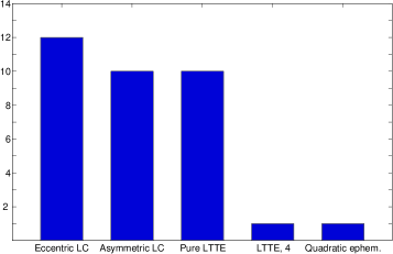
Figure 3: Number of system of each kind from our set of 100 brightest SMC eclipsing binaries (see the text for details).

5 A little statistics

We have manually checked the first one hundred brightest eclipsing binaries from the OGLE III catalogue located in the SMC or its vicinity. These brightest stars have the largest probability to contain the third components (see e.g. Duchêne & Kraus 2013). Hence, we tested the hypothesis of period changes and selected the most pronounced examples of periodic modulation of the orbital periods. Moreover, for some other systems also the other phenomena were detected. These findings are summarized below in Fig. 3.

Among these one hundred stars we have found 11 systems showing LTTE modulation (see the previous Section), twelve systems with obviously eccentric LC, and 10 systems with obviously asymmetric LC shape. One system was classified as a mass-transfer system due to the rapid quadratic ephemerides (OGLE-SMC-ECL-1232), however it is not sure whether such a behaviour is not only a very long-term periodic variation. The rest of the stars show either no variation of their orbital periods or their modulations were still questionable and more data are needed for a final confirmation.

Table 4: Heliocentric minima of the systems used for the analysis.

Star	HJD - 2400000	Error	Type	Filter	Source
$\#$0850	50751.05396	0.00547	Prim	I	OGLE II
$\#$0850	50751.55310	0.00331	Sec	I	OGLE II
$\#$0850	51098.02700	0.00086	Prim	I	OGLE II
$\#$0850	51098.52062	0.00408	Sec	I	OGLE II
…

This table is available in its entirety as a machine-readable table. A portion is shown here for guidance regarding its form and content.

6 Results and discussion

The methods for analysing eclipsing binary are nowadays classical and used almost routinely. However, any such kind of analysis can still bring new and surprising results, especially when applying to some new group of targets. And this can be the case also for this study, which presents the first analysis of the period changes of binaries located in the SMC galaxy.

The classical hypothesis of the light-travel time effect was applied to the 14 selected eclipsing systems from the SMC and we found out that there are probably the third components with rather short orbital periods of couple of years. Moreover, one system was also classified as a candidate for a quadruple. Our focus on the bright (i.e. massive) stars was justified due to the strong correlation between the multiplicity and the masses, as discovered via a study of galactical populations (see e.g. Raghavan et al. 2010). However, at this point it is necessary to emphasize that it is not clear whether all of these stars belong to the SMC galaxy or is it just a coincidence that they lie in the same direction and are members of the Milky Way (however, it is very unlikely because all of them have the distance moduli $>$10 mag).

The presented analysis showed that the predicted third bodies found via the period changes have rather high masses in general, but this is due to the fact that also the eclipsing binary components are massive ones. Another effect which can also play a role is a fact that only a modulation with higher amplitudes are being detected in the data we were using from various databases. We deal here with the stars of the highest luminosity, the highest mass and of the earliest spectral type in the SMC, hence also the third bodies should be massive. This finding was supported by the fact that also large fractions of the third light were usually detected in the light curve solutions and these two numbers well coincide with each other for most of the systems in our sample.

Obviously, we can ask whether in galaxies like SMC is e.g. the multiplicity fraction the same as derived in our Milky Way. Certainly, there arises several selection effects of our method and also some limitations of the available data. First of all, we have only very limited data coverage, of about 20 years in maximum. Hence, also our estimated periods of the third bodies should be of several years to two decades. Shorter orbital periods are rather hard to detect in the available data. From different investigations (e.g. Duquennoy & Mayor 1991, Tokovinin 2008, or Raghavan et al. 2010) there arises that the period distribution of the outer orbits tend to have its maximum even at longer periods. Therefore, we are able to detect here only a small fraction of the true triple systems (tip of the iceberg). Another selection effect should arise from the fact that our method prefers more massive tertiary components (causing larger LTTE amplitudes), while the less massive probably remain undetected. Nevertheless, we can still summarize that our derived multiplicity fraction of about 10% is very similar to that one found by Borkovits et al. (2016) for the galactic population located in the Kepler field. The mass distribution of the two samples is very different (hence also its multiplicity), but with the super precise Kepler data one is able to detect also such triples, which would easily be missed by this method in our sample.

Another finding resulted from our study is the fact that the gravity perturbing effects of the third bodies on the eclipsing binary orbits are generally only very weak. Besides the classical LTTE effect and its dynamical analogy for much closer systems (Borkovits et al., 2016), also the longer-period effects should be present in the three-body system. This is for example the precession of both orbits due to the third body. Most pronounced is typically the change of inclination of the inner eclipsing pair. We are aware of the fact that such systems (called transient eclipsing binaries) exist even in the OGLE database, see e.g. Graczyk et al. (2011) with 17 such systems located in LMC, or new study by (Juryšek, 2017) with a few dozens of such systems. However, the problem is that this effect depends on the period ratio $P_{3}^{2}/P$ (Söderhjelm, 1975), see the last column in Table 3, where one can see that this effect is only very slow to hope finding any evidence for that in upcoming years in our systems. Also the interferometry is out of the game, therefore only the spectroscopy can be used as an independent method for finding the additional bodies in the selected systems.

7 Conclusion

A set of fourteen luminous eclipsing binaries in SMC were analysed resulting in a third-body hypothesis. Some dedicated observation of these systems would be very welcome. This especially applies for the interesting quadruple system OGLE-SMC-ECL-4024, or the systems with very short period $p_{3}$ and high level of the third light (like $\#$1403, $\#$2036, or $\#$2639).

References

- Borkovits et al. (2016) Borkovits, T., Hajdu, T., Sztakovics, J., et al. 2016, MNRAS, 455, 4136
- Davies et al. (2015) Davies, B., Kudritzki, R.-P., Gazak, Z., et al. 2015, ApJ, 806, 21
- Duchêne & Kraus (2013) Duchêne, G., & Kraus, A. 2013, ARA&A, 51, 269
- Duquennoy & Mayor (1991) Duquennoy, A., & Mayor, M. 1991, A&A, 248, 485
- Faccioli et al. (2007) Faccioli, L., Alcock, C., Cook, K., et al. 2007, AJ, 134, 1963
- Gies et al. (2015) Gies, D. R., Matson, R. A., Guo, Z., et al. 2015, AJ, 150, 178
- Graczyk et al. (2011) Graczyk, D., Soszyński, I., Poleski, R., et al. 2011, AcA, 61, 103
- Hilditch et al. (2005) Hilditch, R. W., Howarth, I. D., & Harries, T. J. 2005, MNRAS, 357, 304
- Hong et al. (2016) Hong, K., Lee, J. W., Kim, S.-L., Koo, J.-R., & Lee, C.-U. 2016, MNRAS, 460, 650
- Irwin (1959) Irwin, J. B. 1959, AJ, 64, 149
- Juryšek (2017) Juryšek, J., Zasche, P., Wolf, M., et al. 2017, A&A, submitted
- Kallrath & Milone (2009) Kallrath, J., & Milone, E. F. 2009, ”Eclipsing Binary Stars: Modeling and Analysis: Astronomy and Astrophysics Library”, Springer-Verlag New York
- Massey (2002) Massey, P. 2002, ApJS, 141, 81
- Massey et al. (2012) Massey, P., Morrell, N. I., Neugent, K. F., et al. 2012, ApJ, 748, 96
- Mayer (1990) Mayer, P. 1990, BAICz, 41, 231
- Pawlak et al. (2013) Pawlak, M., Graczyk, D., Soszyński, I., et al. 2013, AcA, 63, 323
- Pawlak et al. (2016) Pawlak, M., Soszyński, I., Udalski, A., et al. 2016, AcA, 66, 421
- Prša & Zwitter (2005) Prša, A., & Zwitter, T. 2005, ApJ, 628, 426
- Raghavan et al. (2010) Raghavan, D., McAlister, H. A., Henry, T. J., et al. 2010, ApJS, 190, 1
- Southworth (2012) Southworth, J. 2012, Orbital Couples: Pas de Deux in the Solar System and the Milky Way, 51
- Söderhjelm (1975) Söderhjelm, S. 1975, A&A, 42, 229
- Terrell & Wilson (2005) Terrell, D., & Wilson, R. E. 2005, Ap&SS, 296, 221
- Tokovinin (2008) Tokovinin, A. 2008, MNRAS, 389, 925
- Udalski et al. (1998) Udalski, A., Szymanski, M., Kubiak, M., et al. 1998, AcA, 48, 147
- van Hamme (1993) van Hamme, W. 1993, AJ, 106, 2096
- Westerlund (1997) Westerlund, B. E. 1997, ”The Magellanic Clouds”, Cambridge University Press, UK
- Wilson & Devinney (1971) Wilson, R. E., & Devinney, E. J. 1971, ApJ, 166, 605
- Wyrzykowski et al. (2004) Wyrzykowski, L.,Udalski, A., Kubiak, M., et al. 2004, AcA, 54, 1
- Zaritsky et al. (2002) Zaritsky, D., Harris, J., Thompson, I. B., Grebel, E. K., & Massey, P. 2002, AJ, 123, 855
- Zasche (2011) Zasche, P. 2011, Information Bulletin on Variable Stars, 5991, 1
- Zasche et al. (2014) Zasche, P., Wolf, M., Vraštil, J., et al. 2014, A&A, 572, A71
- Zasche et al. (2016) Zasche, P., Wolf, M., Vraštil, J., Pilarčík, L., & Juryšek, J. 2016, A&A, 590, A85