Long-term Periodicities of Cataclysmic Variables with Synoptic Surveys

Abstract

A systematic study on the long-term periodicities of known Galactic cataclysmic variables (CVs) was conducted. Among 1580 known CVs, 344 sources were matched and extracted from the Palomar Transient Factory (PTF) data repository. The PTF light curves were combined with the Catalina Real-Time Transient Survey (CRTS) light curves and analyzed. Ten targets were found to exhibit long-term periodic variability, which is not frequently observed in the CV systems. These long-term variations are possibly caused by various mechanisms, such as the precession of the accretion disk, hierarchical triple star system, magnetic field change of the companion star, and other possible mechanisms. We discuss the possible mechanisms in this study. If the long-term period is less than several tens of days, the disk precession period scenario is favored. However, the hierarchical triple star system or the variations in magnetic field strengths are most likely the predominant mechanisms for longer periods.

1 Introduction

A cataclysmic variable (CV) is an accreting binary system composed of a white dwarf (WD) as primary and a low mass companion. In general, when the companion fills its Roche lobe, the mass flow stream passing through the inner Lagrangian point ($L_{1}$) generates an accretion disk around a non-magnetic WD. On the other hand, only a truncated disk can be formed in an intermediate polar (DQ Her type), a subclass of CVs with a highly magnetic WD. The WD in the polar (AM Her type) system has an even higher magnetic field that can prevent the formation of the accretion disk. The variability on different time scales of CV systems is caused by different mechanisms. The orbital periods of CVs typically range from 70 min to 24 h, which is strictly related to the binary separation and mass ratio. A census on the orbital period distribution of CVs reveals a period gap of approximately $2-3$ h (e.g., Warner, 1995), which is explained by the evolution scenarios of CVs.

The variation with a time scale longer than a day is typically called the superorbital or long-term variation in CV systems. Long-term variation has been detected in only a few CVs, and this has been neglected in subsequent research. Kafka & Honeycutt (2004) studied 100 CVs using the structure function to characterize the time scales of the long-term variabilities. However, no further results and the implications behind the long-term variabilities were addressed in this study. Various types of mechanisms were proposed to explain the long-term variations of CVs. For example, Thomas et al. (2010) discovered a long-term modulation with a period of $4.43\pm 0.05$ d in cataclysmic variable PX And through eclipse analysis, which was considered to be the disk precession period that triggers the negative superhump in this system. On the other hand, from the analysis of eclipse time variations in eclipsing binary DP Leo, a third body with an elliptical orbit and a period of $P=2.8\pm 2.0$ yrs was found by Beuermann et al. (2011). Honeycutt et al. (2014) discovered a period of $\sim$ 25 d oscillations, regarded as the result of accretion disk instability in V794 Aql during its small outbursts. Warner (1988) proposed that the cyclical variations of the orbital periods (on the time scale of years to decades) for some CVs are related to their quiescent magnitudes and outburst intervals, and the variations were inferred as the effect of the solar-type magnetic cycle of the companion. Kalomeni (2012) discovered several polars exhibiting long-term variability with a time scale of hundreds of days, likely caused by the modulation of the mass-transfer rate owing to the magnetic cycles in the companion stars.

Previous studies on the long-term periodicities of CVs are sporadic. With the help of recent large synoptic surveys, we are able to search for and further characterize the long-term variations of the CVs systematically. In Section 2, we introduce the synoptic survey projects we utilized, and the corresponding intensive observations made using the Lulin One-Meter-Telescope (LOT). Descriptions of our analysis method for the long-term periodicity of the sources are presented in Section 3. The possible mechanisms driving the long-term variability and further implications are presented in Section 4. In Section 5, we summarize the long-term periodicities from our results and discuss some of the previous studies related to the sources.

2 CV Catalog, Synoptic Surveys and Observations

The CVs selected for this study are from the catalog by Downes et al. (2006). The data used for this study are from two surveys: the Palomar Transient Factory (PTF) and the Catalina Real-Time Transient Survey (CRTS). In addition, the LOT, a small telescope capable of intensive observations, was utilized for finding the orbital periods of the targets that were unknown before this study.

2.1 CV Catalog for Source Matching

The CV catalog produced by Downes et al. (2006) (hereafter Downes’ catalog) is taken as a reference catalog for our study (see Downes et al., 2001, for the catalog description). The latest version of the catalog contains 1830 sources, including 1580 CVs and 250 non-CVs. The catalog used the General Catalogue of Variable Stars (GCVS) name as the source identifier. However, some of the sources have no GCVS names, and so the constellation name of the sources was adopted as the identifier. In this study, if multiple sources without GCVS names are in the same constellation, then the constellation name with distinct numbers were adopted as the project name of the source (e.g., UMa 01 for one of the CVs in the constellation Ursa Major). We used the Downes’ catalog for our matching process and then retrieved the light curves of the matches.

2.2 Palomar Transient Factory

The PTF (Law et al., 2009; Rau et al., 2009) project began observing in 2009. The Samuel Oschin Telescope, a 48-in Schmidt telescope with Mould R, SDSS g^′, and several H-$\alpha$ filters was adopted for the survey. The PTF and its successor intermediate PTF (iPTF) projects were accomplished in March 2017. A 7.9 square degree field of view was achieved with the camera configuration of PTF and iPTF. The next generation of the PTF project, called the Zwicky Transient Facility (ZTF), with its many upgrades in software and hardware, will be operated in mid-2017.

The software pipelines were readied for the real-time discoveries of transients (Masci et al., 2017) and for the generation of source detections (IPAC pipeline, Laher et al., 2014). The IPAC pipeline was developed by the Infrared Processing and Analysis Center (IPAC), which reduced the images and generated the detection catalogs on a frame basis. The detection catalogs are stored in the IRSA archive. We extracted the data from the local copies of the full photometric catalogs in IPAC. Metadata tables with information from the catalog headers were created for accessing the photometric data quickly. The light curve of a specific source could be retrieved out of the total of $\sim 24$ Terabytes within 2 min via our data retrieval pipeline. Figure 1 shows a flowchart of the data-retrieval pipeline. A large area of the sky has been observed by the PTF project. The observation numbers in the density map of sky covered by PTF/iPTF are shown in Figure 2.

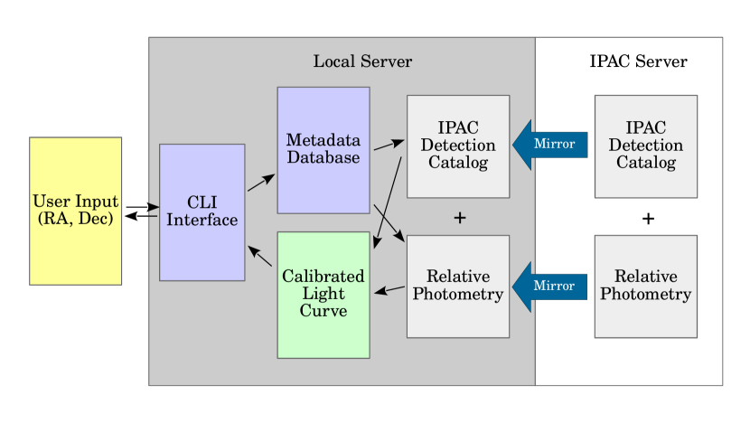
Figure 1: Data flowchart of the light-curve-retrieval process for PTF. IPAC data-processing pipeline (Laher et al., 2014) reduces the survey images, and generates IPAC detection catalogs and relative photometry for each frame (right panel). Middle panel: programs, metadata database and mirrors of the processed data in our local server. The metadata database is generated to store the header information of the IPAC detection catalogs, and is used to speed up the data retrieval process. A command line (CLI) interface was made for users to retrieve the calibrated light curve for a specific source. The speed of the light-curve-retrieval process is increased by a significant factor in this implementation.

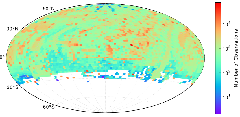
Figure 2: Observational distribution of PTF survey. Each tile in the plot represents a PTF field, and is color-coded with the number of observations in the PTF photometric database. Only R band data are presented. The plot is in equatorial coordinates with the Hammer projection. Observations are absent in the Southern Equatorial Hemisphere (Decl.$<-30^{\circ}$) because of the observing limit of Palomar Mountain site.

2.3 Catalina Real-Time Transient Survey

The CRTS project is conducted by analyzing data from the Catalina Sky Survey (CSS), which is originally designed for the study of asteroids. The CRTS team made use of the photometric data for studying the transient sky (Drake et al., 2009; Mahabal et al., 2011; Djorgovski et al., 2012). The data was gathered using three telescopes in Northern and Southern Hemispheres, including the Catalina Sky Survey (CSS, 0.7m), the Mt. Lemmon Survey (MLS, 1.5m), and the Sliding Springs Survey (SSS, 0.5m). No filter was adopted for the survey to maximize the discovery of asteroids. The CRTS data is available to the public through the Catalina Surveys Data Release 2 (CSDR2) website. The calibrated light curves can be accessed by users through the interface.

2.4 Lulin One-Meter Telescope

The orbital periods of the CVs are essential to the discussion on the mechanism of their long-term periodicities. For our sources of interest, only a portion of them have known orbital periods, as presented in Downes et al. (2006) and references therein. To investigate the targets with unknown orbital periods, we used the Lulin One-Meter Telescope, located in central Taiwan, to perform short-cadence observations. The LOT is a telescope with a field-of-view (FOV) of $11^{\prime}\times 11^{\prime}$. The limiting magnitudes with 5 min exposures are approximately $20-20.5$ mag in V and R bands. We used the R-band filter for our short-cadence observations. The 3 sources we observed with LOT are presented in Table 2.4.

Table 1: Observation log of our LOT observations

Source	Nights	Cadence	Exposure	Filter	$N$
	(day)	(second)	(second)
UMa 01	5	210	200	R	403
CT Boo	4	210	200	R	140
Her 12	2	310	300	R	105
Note: Cadence is the planned observation interval between each of the each frames, and is possibly affected by weather conditions or the instrument. $N$ is the number of the observations.

3 Data Analysis

3.1 Photometric Calibration

The photometric systems of PTF and CRTS are different. The light curves from the PTF repository are in the Mould R band. The data retrieved from the CSDR2 are in white light (unfiltered). To calibrate the difference between the systems, a linear relation between the PTF and CRTS systems was assumed in our analysis. The linear regression to find the cofficients of the line is described as: $M_{\mathrm{PTF}}=A\times M_{\mathrm{CRTS}}+B$, where $M_{\mathrm{PTF}}$ is the $R$ band magnitude measured by the PTF, and $M_{\mathrm{CRTS}}$ is the white-light magnitude measured by the CRTS. The slope $A$ and the intercept $B$ were fit across the magnitudes of different reference stars in the nearby regions of the CVs. Most of the resulting fit parameters $A$ and $B$ are consistent across the entire data set. The magnitudes of the CVs were shifted to the PTF photometric system by the linear relation with the best-fit parameters. The photometric results from the relative photometry are sufficient for further temporal analysis. Therefore, global calibration on the photometric systems is not necessary.

3.2 Timing Analysis

We regarded the data from PTF as the major data set, and the data from CRTS as supplemental. We cross-matched the Downes’ catalog and the PTF database, and found that 344 CVs have PTF photometric data. The spatial distribution of the matches, along with all the CVs in the Downes’ catalog, are shown in Figure 3. About 22% of the CVs in Downes’ catalog have a PTF counterpart. This is because the photometric catalogs of the PTF contain mostly fields in the non-Galactic plane, owing to the difficulties in processing Galactic-plane data and the restrictions inherent to the aperture photometric pipeline.

Matched CVs with only a few observations are not sufficient for studying their timing properties. Therefore, we selected the light curves with more than 100 observations for further investigation. About 100 of the matched CVs satisfied this criterion. These light curves were combined with their corresponding light curves in CRTS. In addition, some of the sources exhibit outbursts in the joint light curves. To avoid the interference from the outbursts, the data points for the outbursts in all the joint light curves were eliminated by visual inspection before the analysis. The dip features that are present in the light curves of cataclysmic variable QZ Ser were eliminated as well, because they are aperiodic. The joint light curves of the 344 selected CVs were then adopted for periodicity analysis. There are 10 CVs found to have long-term periodicities. The joint light curves of these 10 CVs are presented in the upper panels of Figure 4, 5, and 6. The total time span, the data points for timing analysis, and the outburst numbers for the light curves are listed in Table 2.

Table 2: Summary of CVs having long-term periodicities

CV Name	RA (J2000)	Dec (J2000)	Alternative Name	Type	$P_{\mathrm{orb}}$	$\sigma_{P_{\mathrm{orb}}}$	$P_{\mathrm{long}}$	$\sigma_{P_{\mathrm{long}}}$	$p({P_{\mathrm{long}}})$	Amp.	Tspan	N	$N_{\mathrm{ob}}$
	(hh:mm:ss)	($\pm$dd:mm:ss)			(min)	(min)	(day)	(day)		(mag)	(day)	(#)	(#)
BK Lyn	09:20:11.20	+33:56:42.3	2MASS J09201119+3356423	DN/NL	107.97	0.07	42.05	0.01	1.88e-20	0.65	3242.92	514	—
CrB 06	15:32:13.68	+37:01:04.9	2MASS J15321369+3701046	NL	—	—	273.98	2.17	1.18e-13	0.11	3443.86	400	1
CT Boo	14:08:20.91	+53:30:40.2	—	NL	230.72	1.78	7.91	1.05	4.11e-04	0.13	2893.00	296	—
					78.65	0.36
LU Cam	05:58:17.89	+67:53:46.0	2MASS J05581789+6753459	DN	215.95	0.0005	256.76	2.10	3.18e-03	0.62	2934.95	363	—
Her 12	15:50:37.28	+40:54:40.0	SDSS J155037.27+405440.0	CV	75.62	0.008	326.81	1.32	4.97e-07	0.18	3033.88	429	1
					173.65	1.57
QZ Ser	15:56:54.47	+21:07:19.0	SDSS J155654.47+210719.0	DN	119.75	0.002	277.72	8.76	9.18e-07	0.09	3308.01	510	2
UMa 01	09:19:35.70	+50:28:26.2	2MASS J09193569+5028261	CV	404.10	0.30	246.84	0.81	8.01e-20	0.44	3251.05	601	1
V825 Her	17:18:36.99	+41:15:51.2	2MASS J17183699+4115511	NL	296.64	2.88	515.55	1.85	3.28e-16	0.16	3069.71	510	—
							9.24	0.05	4.51e-16	0.18
V1007 Her	17:24:06.32	+41:14:10.1	1RXS J172405.7+411402	AM	119.93	0.0001	170.59	0.12	2.13e-18	0.90	3069.71	507	—
VW CrB	16:00:03.71	+33:11:13.9	USNO-B1.0 1231-00276740	DN	—	—	142.60	0.24	1.92e-21	0.87	3271.19	351	$>$10

Note. — The numbers in bold face indicate the values derived in this work. Multiple possible orbital periods present in CT Boo and Her 12, and they are listed in the table accordingly.

^a CV name: name designated in this project; ^b Alternative name: the source name in 2MASS, SDSS, ROSAT bright source catalog (1RXS) or USNO B1.0 catalogs; ^c Type: the type of CVs designated in Downes et al. (2006)(NL: nova-like, DN: dwarf nova, AM: AM Her (polar)); ^d $P_{\mathrm{orb}}$: orbital periods; ^e $\sigma_{P_{\mathrm{orb}}}$: errors of orbital periods; ^f $P_{\mathrm{long}}$: long-term periods derived in this work; ^g $\sigma_{P_{\mathrm{long}}}$: errors of long-term periods derived in this work; ^h $p(P_{\mathrm{long}})$: the $p$-value of the long-term period; ⁱ Amplitude: peak-to-peak magnitude difference from the fit light curve; ^j $T_{\mathrm{span}}$: total time span; ^k $N$: number of observations excluding outbursts and dips; ^l $N_{\mathrm{ob}}$: number of outbursts observed with PTF and CRTS; ^m Ringwald et al. (1996); ⁿ Sheets et al. (2007); ^o Thorstensen et al. (2002); ^p Ringwald & Reynolds (2003); ^q Greiner et al. (1998)

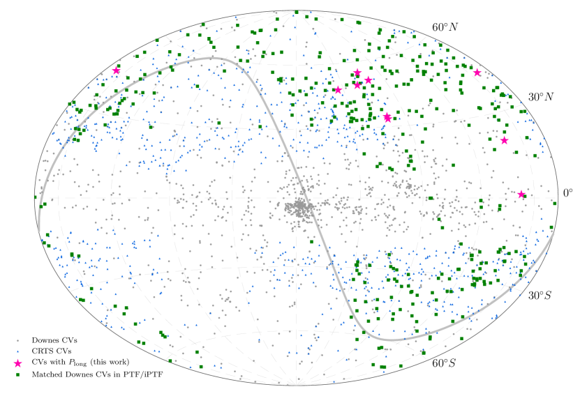
Figure 3: Spatial distribution of Galactic CVs found by various previous studies and in this study. Green squares represent the matched sources in PTF with the catalog from Downes et al. (2006). Gray filled circles are targets in Downes et al. (2006) catalog but not matched in the PTF survey. Blue triangles are the CV candidates with the CRTS project, proposed by Drake et al. (2014). The ecliptic plane is drawn with a gray line. This figure is presented in Galactic coordinates with the Hammer projection.

Figure 4: Upper panel – light curves from PTF and CRTS. Magenta: PTF; blue: CRTS; gray: data points of outbursts or dips eliminated in the analysis. Middle panel – Lomb-Scargle periodogram of the joint light curve (upper), and the window function (lower, normalized). Blue bar in the top of the panel shows the error from the Monte Carlo simulation. Green arrows show the values of the periods of our interests. Orange dashed line indicates the 95% confidence level ($P_{95\%}$). The red dashed vertical line indicates the period used for the folded light curve in the lower panel. Lower panel – gray: folded light curves; red: binned light curves with 15 bins to address the modulation; blue: the fit line with two sinusoidal components.

Figure 5: Light curves (upper panel), Lomb-Scargle periodogram of CVs (upper of middle panel) and window function (lower of middle panel), and folded light curves (lower panel) (continued). The descriptions and labels are the same as in Figure 4.

Figure 6: Light curves (upper panel), Lomb-Scargle periodogram of CVs (upper of middle panel) and window function (lower of middle panel), and folded light curves (lower panel) (continued). The descriptions and labels are the same as in Figure 4.

To study the timing properties of these CVs, the Lomb-Scargle periodogram (LS, Lomb, 1976; Scargle, 1982) was adopted to search for the periodicities, and the method of Phase-Dispersion Minimization (PDM, Stellingwerf, 1978) was used to cross-check the candidate periods. The periods obtained from these two methods are consistent to each other. In this paper, we only present the results from LS. For the same FOV, the observation schedules of PTF and CRTS are not regular and not fixed. Therefore, there are many observation gaps in the light curves. Aliases can be observed in the power spectra owing to the gaps in the observations, and this makes analyzing the light curves difficult. To distinguish and eliminate the aliasing introduced by the windows, the periodogram of the observation windows are plotted against the source periodogram, as demonstrated in the lower graphs of the middle panels in Figure 4, 5, and 6.

A summary of the possible CVs with the long-term periodicities are listed in Table 2. For the LS periodogram, the $p$-value is frequently adopted to represent the detection significance of a periodic signal. The $p$-value is defined as the probability that the periodogram power can exceed a given value $P_{i}$, expressed as $\mathrm{Prob}(P>P_{i})$, and can be expressed as:

$$p\equiv\mathrm{Prob}(P>P_{i})=\left(1-\frac{2P_{i}}{N-1}\right)^{\frac{N-3}{2}}$$ (1)

where $N$ is the total number of observations (Zechmeister & Kürster, 2009).

To derive the corresponding uncertainty of the most probable long-term period, Monte Carlo simulations were conducted $10^{4}$ times under the assumption that the observational errors are Gaussian distributed. On the basis of the observed magnitudes and corresponding errors of each CV, we generated $10^{4}$ simulated light curves. The root-mean-square values of the peak values in the power spectra were adopted as the statistic errors of the derived periods. The errors of the periods are also listed in Table 2.

Light curves were folded with the most probable periods in the power spectra, as shown in the lower panels of Figure 4, 5, and 6. To show the profiles of the long-term modulations, we binned the folded light curves into 15 phase intervals, and fit each of them with a two-sinusoidal function, which is given as:

$$M=c_{1}\sin(2\pi\phi+c_{2})+c_{3}\sin(4\pi\phi+c_{4})+c_{5}$$ (2)

where $\phi$ is the phase of the folded light curve, $M$ is the corresponding magnitude, and $c_{1}$ through $c_{5}$ are the fit cofficients.

The scattering of the points in the folded light curves may be caused by the original photometric uncertainties. However, the variations from shorter time scales, such as the orbital modulations, contribute to the light curves; therefore, these variations cannot be neglected. We tried to fold the original light curves of the CVs with their known constant orbital periods; however, this failed in reconstructing their orbital profiles.

3.3 Lulin One-Meter Telescope Observations

The images we took using the LOT were reduced by NOAO IRAF packages. The images were processed by subtracting the master bias and dark frames. Then, the flat-field correction was applied for correcting the pixel-dependent instrument response. Point spread function (PSF) fitting was performed on the images using DAOPHOT to obtain accurate photometric results. In the light curves derived from the PSF fitting, different trends exist between different days. The mean value of the data in each day was subtracted for reducing the interference of the trend. The detrended light curves are presented in Figure 7. Moreover, the LS periodogram was applied for searching for periodicities in the light curves. The folded light curves were produced by folding the detrended light curves with the best determined periods. The power spectra and the folded light curves are shown in Figure 7. The significance levels are indicated by the $p$-values as well. A summary of the results is shown in Table 3.

Table 3: Periodicities in short-cadence observations

Source	$P_{\mathrm{opt}}$	$\sigma_{P_{\mathrm{opt}}}$	$P_{\mathrm{peak}}$	$p$-value	N
	(min)	(min)
UMa 01	404.10	0.30	36.54	3.74e-18	403
CT Boo	230.72	1.78	9.80	2.99e-05	140
	78.65	0.36	9.49	4.29e-05	140
Her 12	173.65	1.57	26.75	1.00e-16	105
	75.62	0.008	19.22	6.02e-11	105
Note: $P_{\mathrm{opt}}$: optical periods, $\sigma_{P_{\mathrm{opt}}}$: errors in periods by Monte Carlo simulations, $P_{\mathrm{peak}}$: peak power in the power spectrum.

Intensive observations were conducted for the unknown orbital periods of the CVs with long-term periodicities. In this study, three CVs, namely UMa 01, CT Boo, and Her 12 were observed and analyzed. UMa 01 (a.k.a. 2MASS J09193569+5028261) shows a modulation with a period of $404.10\pm 0.3$ min. CT Boo exhibits two significant periodic signals: $229.13\pm 7.02$ and $79.55\pm 0.51$ min. In addition, two significant periods were found in Her 12 (a.k.a. SDSS J155037.27+405440.0): $75.62\pm 0.008$ and $173.65\pm 1.57$ min. These periods for the three CVs are all located in the normal orbital period range of CVs. However, for the CVs with multiple periodicities, further investigation is required to distinguish and confirm the orbital periods. Besides, it is not easy to distinguish them if the modulations in the folded light curves are orbital humps or superhumps (defined below in Section 4.1). We assume that these periods are the possible orbital periods in the discussion that follows.

Figure 7: Folded short cadence light curves of (a) UMa 01, (b) CT Boo, and (c) Her 12. Upper panels show the detrended light curves in the available data segments. Middle panels present the Lomb-Scargle periodogram of the CVs. The magenta dashed line denotes the L-S power with 95% confidence level, and red dashed lines denote the periodic signals used for the folded periods. Lower panels show the folded light curves with the best periods in the Lomb-Scargle periodogram. Gray dots are the folded light curves. Purple points indicate the binned light curves and errors. Blue curves represent the modulation trends with fits to a function with two sinusoidal components.

4 Possible Mechanisms of Long-term Periodicity

Long-term periodicities are not frequently observed in close binary systems. However, some X-ray binaries (XBs) exhibit long-term periodicities. Kotze & Charles (2012) summarized several possible mechanisms for the long-term variability of XBs, and some of the scenarios may also be applicable to CV systems. The distribution of the long-term periodicities in our study is presented in Figure. 8. The long-term periods that are associated with the superhumps of other CVs were gathered from different literature, and were plotted for comparison. The long-term periodicities of the low-mass X-ray binaries (LMXBs) in Kotze & Charles (2012) were plotted, as well. In this section, we list and discuss some of the possible mechanisms that cause the long-term variations in CVs.

4.1 Precession of Accretion Disk

CVs are named for their cataclysmic phenomena. The state change of the accretion disk of CVs may cause their emission flux to change. In addition to the orbital modulations, variations in the periods of a few percent longer or shorter than the orbital periods are called positive and negative superhumps, respectively. Superhump was first found in the SU UMa type (a subtype of dwarf novae (DNe)) of CVs. During the superoutbursts of a SU UMa type star, a periodic hump rather than an orbital hump appears and this was called superhump (Warner, 1985; Vogt, 1980; Warner, 1995). Besides the SU UMa type of CVs, some of the VY Scl type of CVs (or anti-dwarf novae), a subtype of nova-like (NL) CV, were detected to have superhump signals. For example, Kozhevnikov (2007) discovered a negative superhump $P_{\mathrm{sh}}$ = 3.771 $\pm$ 0.005 h in KR Aur, a VY Scl NL CV. In addition to the SU UMa and NL systems, superhumps were also observed in the intermediate polar (IP, or DQ Her type of CVs). Woudt et al. (2012) found superhumps in CC Scl, an IP system, with a period of $P_{\mathrm{sh}}$ = 1.443 h, $\sim 4.3\%$ longer than its orbital period $P_{\mathrm{orb}}$ = 1.383 h.

In general, it is believed that the positive/negative superhump periods are the beat periods of the orbital period and the precession period of the accretion disk. For a positive superhump, the size of the accretion disk is growing as mass transferring from the companion. When the radius of the accretion disk is larger than the 3:1 resonance radius of the binary, the accretion disk becomes asymmetric and exhibits apsidal precession (Whitehurst, 1988; Osaki, 1989, 1996). Whitehurst & King (1991) proposed that this criterion can be achieved only for CV systems with mass ratio $q\equiv M_{\mathrm{d}}/M_{\mathrm{c}}<0.25-0.33$, where $M_{\mathrm{c}}$ and $M_{\mathrm{d}}$ are the masses of the accretor and donor, respectively. A positive superhump is a consequence of coupling disk apsidal precession and orbital motion with the beat period for these two types of periodic motions. On the other hand, a negative superhump is believed to be the result of coupling between orbital motion and disk nodal precession.

The period excess of a superhump is defined as follows:

$$\epsilon\equiv\frac{P_{\mathrm{sh}}-P_{\mathrm{orb}}}{P_{\mathrm{orb}}}$$ (3)

In general, the period excess for a positive superhump is in the range of $1-7\%$. The period deficit for a negative superhump is about half of a excess of the positive superhump (Patterson, 1999). Therefore, the period ranges of the disk precession can be derived with known $P_{\mathrm{orb}}$ and $P_{\mathrm{sh}}$. Figure 9 presents our results in a plot of $P_{\mathrm{orb}}$ vs. $P_{\mathrm{long}}$.

In general, LMXBs are similar to CVs (Charles, 2002). LMXBs have low mass companions; therefore, some of them possibly satisfy the mass-ratio criterion that introduces the disk precession. The results of some long-term variability studies on LMXBs (Kotze & Charles, 2012) and CVs (see Table 4) were gathered and included with our Figure 9 results for comparison. In Figure 9, the gray area and iris hatched areas denote the possible regions of the long-term periods in the positive ($P_{\mathrm{sh+}}$) and negative superhump ($P_{\mathrm{sh-}}$) systems, respectively. In this study, only the long-term periods of CT Boo and V825 Her are the possible precession periods (see Section 5 for more details).

If the long-term period is the disk precession period, the period is confined by its orbital period. For an extreme case of CV, say $P_{\mathrm{orb}}=1$ day, the maximum apsidal precession period and the maximum nodal precession period are approximately 101 d and 199 d, respectively. We conclude that if the long-term periodicities are longer than 200 d, then the possibility of the long-term period being the disk precession can be completely eliminated.

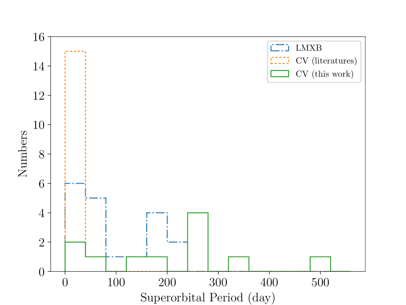
Figure 8: Histogram of known superorbital periods in close binary systems. Blue dashed dots: LMXBs from Kotze & Charles (2012); orange dots: CVs from various studies (see Table 4); green line: CVs of this study.

4.2 Hierarchical Triple Star

Some of the close binaries, such as LMXBs and CVs, were reported in triple or even multiple star systems. Chou & Grindlay (2001) indicated that the superorbital modulation period $P=171.033\pm 0.326$ d is found in LMXB 4U 1820-30 with a limit of the period derivative $|\dot{P}|<1.03\times 10^{-4}$ d d^-1. The luminosity modulation and its long-term stability suggest that it is a hierarchical triple star system. Beuermann et al. (2011) discovered a third star of mass $M_{3}$ = 6.1 $\pm$ 0.5 $M_{\mathrm{J}}$ orbiting the eclipsing binary DP Leo with orbital period $P_{3}$ = 28 $\pm$ 2 yrs. Potter et al. (2011) studied the eclipsing polar UZ For and found that, except for the binary orbital period $P_{\mathrm{orb}}=0.088$ d, there are also two long-term cyclic variations: $P_{3}$ = 16 $\pm$ 3 yrs and $P_{4}$ = 5.25 $\pm$ 0.25 yrs. Moreover, they were interpreted as two giant exoplanets, with masses of $M_{3}=6.3\pm 1.5M_{\mathrm{J}}$ ($M_{J}$ is the Jovian mass) and $M_{4}=7.7\pm 1.2M_{\mathrm{J}}$, being companions to the binary system. Chavez et al. (2012) detected a periodicity of $\sim 900$ d in the light curves of FS Aur, and then used a numerical simulation of a third body with sub-stellar mass orbiting around the binary to reproduce the long-term modulation in the binary eccentricity variation.

A triple star is expected to form in high number density regions, such as the core of globular clusters, which may aid the capture process by a CV system. Trenti et al. (2008) performed an N-body simulation for investigating the formation of triple systems in star clusters. Their results yielded that the probability of forming triple stars in the center of a star cluster is only two orders lower than that of binaries, which is comparably prominent. A small third body could significantly affect the eccentricity of the inner binary, and then result in a mass-transfer-rate change of the CV system. This long-term periodicity is known as Lidov-Kozai oscillation (Lidov, 1962; Kozai, 1962). The relation between the outer third star and the inner binary can be expressed by the relation proposed by Mazeh & Shaham (1979):

$$P_{\mathrm{long}}=P_{1,2}\left(\frac{a_{3}}{a_{1,2}}\right)\frac{m_{1}+m_{2}}{m_{3}},$$ (4)

where $P_{\mathrm{long}}$ is the long-term periodicity, $P_{1,2}$ is the inner binary orbital period, $m_{1}$ and $m_{2}$ are the primary and the secondary masses, $m_{3}$ is the mass of the third star, $a_{1,2}$ is the separation of the inner CV, and $a_{3}$ is the separation between the CV and the third star. An approximation can be expressed as follows:

$$P_{\mathrm{long}}\approx\alpha\frac{P_{\mathrm{3}}^{2}}{P_{1,2}}\frac{m_{1}+m_{2}+m_{3}}{m_{3}}(1-e_{\mathrm{out}})^{3/2},$$ (5)

where $e_{\mathrm{out}}$ is the eccentricity between the third star and the inner binary, and $\alpha$ is a dimensionless quantity from the three-body Hamiltonian. When the outer eccentricity is fixed, and there is no mass transfer between the inner binary and outer star, then Equation 5 can be expressed as follows:

$$P_{\mathrm{long}}=K\frac{P_{\mathrm{3}}^{2}}{P_{1,2}},$$ (6)

where $K$ is a constant of order unity, and Chou & Grindlay (2001) take $K\simeq 1$ as an approximation (for different inclination angles, $K$ taken as a factor of 2 smaller or larger is applicable). For example, in 4U 1820-30, $P_{\mathrm{long}}=171.033$ d and $P_{\mathrm{orb}}=685$ s. Using Equation 6, and assuming $K=1$, this results in $P_{3}=1.18$ d, which is considerably longer than the orbital period of the inner binary, and so the hierarchical order of the triple system is reasonable. Therefore, we could conclude that the hierarchical triple star system is one of the possible scenarios leading to long-term periodicities in CVs.

4.3 Magnetic Variation of the Companion Star

Most companions in CVs are late-type stars. The convective zone in a late-type star (G, K, or M type) yields a strong magnetic field through the well-known dynamo process. The strength of the magnetic field is related to the rotation of the star. Under the same rotation speed, a star of the latter spectral type would yield stronger magnetic field by the dynamo effect (Durney & Robinson, 1982; Robinson & Durney, 1982). Because of the stronger magnetic field strength, the accretion process in the CV system is possibly affected.

Long-term modulations of orbital period variations have been found and studied in some eclipsing binaries. Applegate (1992) proposed that the torque generated from the magnetic variation of the companion may induce such a long-term periodicity. Meyer-Hofmeister et al. (1996) studied the outburst frequency of dwarf novae and found a cycle of 18 yrs in SS Aur and 7 yrs of SS Cyg. They inferred that these cycles are related to the magnetic field variation of the companion. Borges et al. (2008) discovered a 36 yr periodic signal in the eclipsing cataclysmic variable HT Cas. The periodicity is likely to be the solar-type magnetic activity of the companion stars. Ak et al. (2001) observed cyclical variations in quiescence magnitude and outburst intervals of 21 dwarf novae, one nova, and one NL star. The probability density functions are peaked at 9.7 yrs for CVs, 7.9 yrs for single main-sequence stars, and 8.6 yrs for all stars.

The distribution of the cycle lengths caused by the magnetic field variations of late-type stars was studied by Suárez Mascareño et al. (2016). Their results reveal that the majority of cycle lengths are in the $2-13$ yr range. For our results in Table 2, the longest period is $P_{\mathrm{long}}=515.52\pm 1.85$ d in V825 Her, which is marginal relative to the aforementioned magnetic time scale. We cannot completely eliminate the possibility of magnetic variation of the companion as a cause of long-term periodicity in CVs. However, for our targets, the chance of magnetic variation is not high according to the revealed period ranges of our targets.

4.4 Other Possibilities

In addition to the above mechanisms for long-term periodicities in CVs, the superoutburst cycle of the SU UMa type of CV sometimes displays periodic-like signals (e.g. Shears, 2009). On the other hand, Šimon (2016) found the periodic-like transition between the high and low states in cataclysmic variable AM Her, and proposed the lifetime of the active region in the companion may contribute to the variation of the accretion rate. In some rare cases, the long-term variation may also possibly be induced by the precession of the jet in XBs (Kotze & Charles, 2012), but the existence of jets in CVs is still controversial. However, Körding et al. (2011) first observed the radio emissions of V3885 Sgr, which is a nova-like cataclysmic variable (NLCV), and the radio emission from V3885 Sgr is regarded as synchrotron emissions from the jet.

Table 4: Long-term periodicities in CVs caused by superhumps

Name	$P_{\mathrm{orb}}$	$P_{\mathrm{sh}}$	$P_{\mathrm{long}}$	Type(sh)	Type	Reference
	(hr)	(hr)	(day)
AH Men	2.95	3.05	3.71	$+$	Nova	Patterson (1995)
DV UMa	2.06	2.14	2	$+$	DN	Vanmunster (2006)
CC Scl	1.38	1.44	1.6†	$+$	Nova	Woudt et al. (2012)
LT Eri	4.08	3.98	5.3	$-$	CV	Ak et al. (2005a)
LQ Peg	3.22	3.42	2.37	$+$	Nova	Rude & Ringwald (2012)
MV Lyr	3.19	3.31	3.6	$+$	Nova	Skillman et al. (1995)
NSV 1907	6.63	6.22	4.21	$-$	NL	Hümmerich et al. (2017)
PX And	3.41	3.51	4.43	$+$	CV	Thomas et al. (2010)
RR Pic	3.48	3.78	1.79	$+$	Nova	Schmidtobreick et al. (2008)
TT Ari	3.30	3.57	1.82	$+$	Nova	Stanishev et al. (2001)
TV Col	5.50	5.20	3.93	$-$	DQ Her	Augusteijn et al. (1994)
UX UMa	4.72	4.48	3.68	$-$	NL	de Miguel et al. (2016)
V1193 Ori	3.43	3.26	2.98	$-$	Nova	Ak et al. (2005b)
V2051 Oph	1.50	1.54	52.5†	$+$	DN	Vrielmann & Offutt (2003)
V603 Aql	3.32	3.47	3.15†	$+$	Nova	Suleimanov et al. (2004)
WZ Sge	1.33	1.37	5.7	$+$	DN	Patterson et al. (2002)
Note: $P_{\mathrm{orb}}$, $P_{\mathrm{sh}}$, $P_{\mathrm{long}}$ are orbital, superhump and long-term disk precession periods, respectively. Type(sh) is the type of superhump: “$+$” for positive superhumps, “$-$” for negative superhumps.
† average value of multiple periodicities

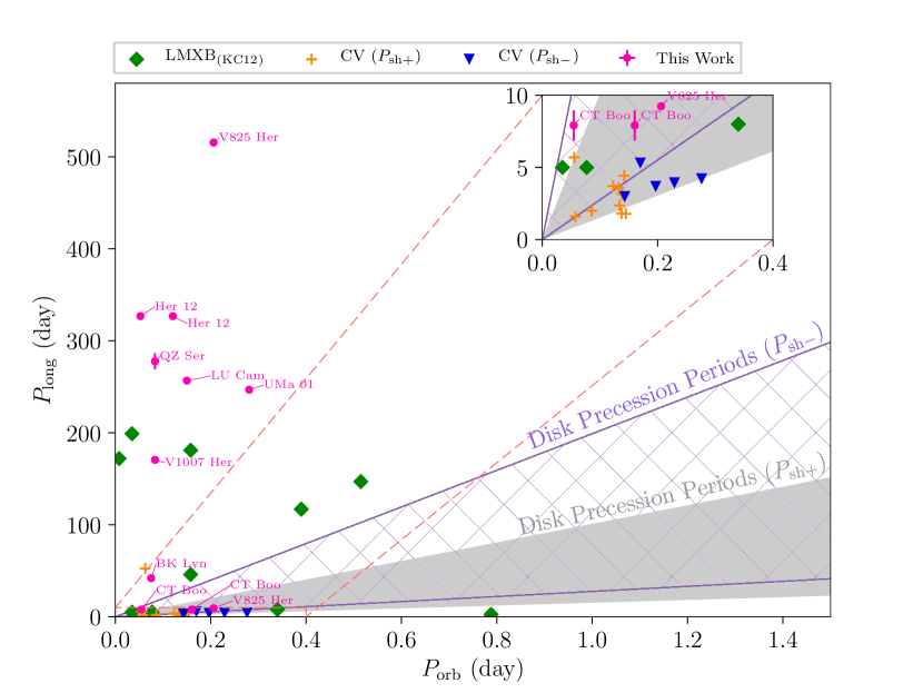
Figure 9: $P_{\mathrm{long}}$ vs. $P_{\mathrm{orb}}$ relations for LMXBs, and CVs. LMXBs data are shown with green diamonds (see Kotze & Charles (2012) (KC12)). If the long-term periods were provided in ranges, the average values are adopted for the plot. CVs from previous studies with long-term periods, which are related to positive and negative superhumps, are in orange crosses and blue triangles, respectively (as listed in Table 4). The filled magenta circles denote the results from our study. The gray area denotes the possible region of disk precession period $P_{\mathrm{prec}}$ with superhump period excess $\epsilon$ in $1-7\%$ range (positive superhump ($P_{\mathrm{sh+}}$)). The iris hatched area represents the region of accretion disk precession period $P_{\mathrm{prec}}$ with period excess of superhump ($\epsilon$) between $-0.5$% and $-3.5$% (negative superhump ($P_{\mathrm{sh-}}$)). The zoomed-in view of the dashed box is in upper right corner of the plot. Only CT Boo and V825 Her are located in the possible regions related to the superhump phenomenon.

5 Long-term modulation for the individual CVs

We have searched for long-term periodicities in approximately 100 CVs from the PTF database (Section 3.2). It turns out that 10 of the targets exhibit obvious periodic signals. We folded the light curves with their best periods, as shown in Figure 4, 5 and 6. The most convincing CVs that possess long-term periods ($P_{\mathrm{long}}$) are discussed in this section. The long-term periodicities discovered in these CVs provide us with some probable implications for their formation mechanisms (see Section 4). We discuss these CVs in the following subsections:

5.1 BK Lyncis (2MASS J09201119+3356423)

BK Lyn (also PG0917+342), a NLCV, which was discovered by Green et al. (1982), has an orbital period of $P_{\mathrm{orb}}$ = 107.97 $\pm$ 0.07 min (Ringwald et al., 1996). Dhillon et al. (2000) found that its secondary is an M5V star from infrared spectroscopy. The accretion rate was estimated as $\dot{M}\sim$ 1 $\times 10^{-9}M_{\odot}/\mathrm{yr}$ assuming a WD mass of 1.2$~{}M_{\odot}$, or $\dot{M}\sim$ 1 $\times 10^{-8}M_{\odot}/\mathrm{yr}$ for WD mass $M_{\mathrm{WD}}$ = 0.4$~{}M_{\odot}$ (Zellem et al., 2009). Kemp et al. (2012) studied 20-yr light curves of BK Lyn and detected two sets of superhump signals. One is 4.6% longer and the other is 3.0% shorter than the $P_{\mathrm{orb}}$. The two superhumps were observed in different light curve stages. They are possibly due to the prograde apsidal precession and retrograde nodal precession of its accretion disk. The long-term period found in our study is $42.05\pm 0.01$ d, which is considerably longer than the long-term period derived from the superhump periods found by Kemp et al. (2012). This suggests that the periodicity is probably not from the precession of the accretion disk. On the other hand, if the long-term periodicity is driven by a third star orbiting the CV system, then the orbital period of the third star will be $P_{3}=1.78$ d (as calculated by Equation 6), which is much longer than the orbital period of BK Lyn.

5.2 CT Boötis

CT Boo shows spectra similar to F-G stars, and no emission lines of hot continuum was observed (Zwitter & Munari, 1994). If the spectrum is dominated by its companion star, owing to the dynamo effect in the convective layer of a late-type star, the magnetic field will be stronger than for other spectral types of stars. However, the long-term period is $P_{\mathrm{long}}=7.91\pm 1.05$ d, which is considerably shorter than the time scale of the stellar magnetic variation (see Section 4.3).

Two possible orbital periods discovered by this study are $P_{\mathrm{orb}}=230.72\pm 1.78$ min and $P_{\mathrm{orb}}=78.65\pm 0.36$ min. With the positive superhump period excess between $1\%$ and $7\%$ and negative superhump period excess between $-0.5\%$ and $-3.5\%$, we calculated the possible accretion disk precession to be $2.45-31.88$ d for $P_{\mathrm{orb}}=230.72$ min, and between 0.83 and 10.87 d for $P_{\mathrm{orb}}=78.65$ min. Therefore, the long-term period found for CT Boo is in good agreement with the disk precession period from the coupling of orbital and superhump periods.

5.3 LU Camelopardalis: 2MASS J05581789+6753459

The orbital period of LU Cam is $P_{\mathrm{orb}}=0.1499686(4)$ d (Sheets et al., 2007) whereas its long-term modulation period is $P_{\mathrm{long}}=265.76\pm 2.10$ d. The possibility of disk precession can be completely eliminated because it exceeds the period limit of 29.84 d for the possible disk precession period. If LU Cam is a hierarchical triple star system, using Equation 6 and assuming $K=1$, the orbital period of the outer third body is $P_{3}\sim 6.20$ d, which is considerably longer than the orbital period of the inner binary. Therefore, the hierarchical triple star is a possible scenario for the long-term periodicity in LU Cam.

5.4 QZ Serpentis: SDSS J155654.47+210719.0

QZ Ser is a dwarf nova system with an orbital period of 0.08316 d, and with a K4 type star as its companion (Thorstensen et al., 2002). If there is superhump-related disk precession, the period should be less than 16.54 d, which is considerably shorter than the long-term period that we obtained ($P_{\mathrm{long}}$ = 277.72 $\pm$ 8.76 d). If QZ Ser is a triple star system, the orbital period of the third star would be $P_{3}\sim 4.81$ d (through Equation 6).

5.5 V825 Herculis: 2MASS J17183699+4115511

V825 Her, also named PG117+413 and 2MASS J17183699+4115511, has an orbital period of $P_{\mathrm{orb}}=4.94$ h discovered by Ringwald (1991). The upper limits of the long-term periods calculated for positive and negative superhump systems are 20.79 d and 40.96 d, respectively. There are two sets of long-term periodicities in the power spectrum of V825 Her. One is $P_{\mathrm{long}}=9.24\pm 0.05$ d, and the other one is considerably longer $P_{\mathrm{long}}=515.52\pm 1.85$ d. These two periods exhibit convincing variations in the folded light curves, as shown in Figure. 5. $P_{\mathrm{long}}=9.24$ d is plausibly explained as the disk precession period; whereas, $P_{\mathrm{long}}=515.52$ d is perhaps caused by the magnetic variation of the companion star (see Section 4.3).

5.6 V1007 Her: 1RXS J172405.7+411402

V1007 Her, discovered by Greiner et al. (1998), is a polar system with an orbital period of $P_{\mathrm{orb}}=119.93\pm 0.0001$ min. Because it is a polar system, the long term modulation is impossibly caused by precession of accretion disk. If the long-term periodicity is caused by a third star, then the orbital period of the third star ($P_{3}$) is about $3.77$ d, much longer than the orbital period of the inner CV, and this becomes a possible mechanism to explain the period of $\sim 170$ d modulation.

5.7 UMa 01: 2MASS J09193569+5028261

UMa 01 (also 2MASS J09193569+5028261) was identified by Adelman-McCarthy et al. (2006) as a CV. The orbital period discovered in this study is $P_{\mathrm{orb}}=404.10\pm 0.30$ min. If there is disk precession in this system, then the precession period would range from $4.29$ to $55.84$ d. However, the long-term period discovered in this study is $P_{\mathrm{long}}=246.84\pm 0.81$ d, which is too large for disk precession. On the other hand, if the long-term periodicity is from a third star orbiting around the CV system, then the orbital period $P_{3}$ would be $8.32$ d, much longer than the orbital period of the inner CV, and so UMa 01 may be a hierarchical triple system.

5.8 Her 12: SDSS J155037.27+405440.0

Her 12 (also SDSS J155037.27+405440.0) was identified as a CV by Adelman-McCarthy et al. (2006). We proposed two candidates of its orbital period based on the LOT observations, $P_{\mathrm{orb}}=75.62\pm 0.008$ min and $P_{\mathrm{orb}}=173.65\pm 1.57$ min. The ranges for the disk precession periods are $0.8$ to $10.45$ d and $1.84$ to $24$ d for $P_{\mathrm{orb}}=75.62$ min and $173.65$ min, respectively. The long-term modulation period discovered in this work is $P_{\mathrm{long}}=43.6\pm 0.29$ d, exceeding both ranges, and thus, this modulation is unlikely to be caused by accretion disk precession. On the other hand, if this source is a hierarchical triple system, then the orbital period of the third companion is $1.51$ d or $2.29$ d for the orbital periods of $75.62$ min or $173.65$ min, respectively. Both of the third-body orbital periods are much larger than the corresponding orbital periods of the CV. Therefore, this triple model is a possible mechanism to explain the long-term variability of Her 12.

5.9 Coronae Borealis 06 & VW Coronae Borealis

CrB 06 (also 2MASS J15321369+3701046) and VW CrB (also USNO-B1.0 1231-00276740) were identified as CVs in Szkody et al. (2006) and Adelman-McCarthy et al. (2006), respectively. Unfortunately, the orbital periods of both CVs remain unknown. Therefore, at the current stage, we cannot speculate on the possible mechanisms of long-term variability for these CVs.

5.10 Summary

We discussed several possible mechanisms to explain the long-term modulations for the CVs that we found in this study. Only the long-term periodicities in CT Boo and V825 Her are possibly caused by the disk precession periods. On the other hand, for the other CVs included in this study, the hierarchical triple systems are conceivable mechanisms for yielding long-term periodicities in CVs. In addition, the magnetic variations of companions in CVs is yet another possible mechanism to cause the long-term variations; nevertheless, the tendency toward longer periods by this mechanism reduces its likelihood as a plausible explanation for the long-term periodicities in this study.

6 Conclusion and prospect

We presented our study on the long-term variations of CVs in this paper. We matched 344 CVs in the CV catalog of Downes with the PTF photometric database. Approximately 100 CVs have more than 100 observations. Among them, 10 of the CVs exhibited long-term periodicities. The long-term periodicities may be caused by one of the following mechanisms: disk precession, the presence of a hierarchical triple-star system, magnetic variation of the companion star, jet precession, and others. We discussed the likelihood of each possible mechanism with respect to our matched CVs. In addition, we found the possible orbital periods for three of the CVs with the short cadence optical observations made by LOT. The ranges of the orbital periods are typical in the orbital period distribution.

With less sparse observations and longer observation time spans, the uncertainties in the long-term periodic signals can be reduced. We look forward to more sophisticated sample of long-term periodicities in CVs when ZTF and other big synoptic surveys are in operation. According to the current plan for ZTF, the Galactic-plane survey will be one of the major parts of the project that may considerably enhance the target number of CVs. We will certainly benefit considerably from next-generation synoptic surveys.

References

- Adelman-McCarthy et al. (2006) Adelman-McCarthy, J. K., Agüeros, M. A., Allam, S. S., et al. 2006, ApJS, 162, 38
- Ak et al. (2001) Ak, T., Ozkan, M. T., & Mattei, J. A. 2001, A&A, 369, 882
- Ak et al. (2005a) Ak, T., Retter, A., Liu, A., & Esenoğlu, H. H. 2005a, PASA, 22, 105
- Ak et al. (2005b) Ak, T., Retter, A., & Liu, A. 2005b, New A, 11, 147
- Applegate (1992) Applegate, J. H. 1992, ApJ, 385, 621
- Augusteijn et al. (1994) Augusteijn, T., Heemskerk, M. H. M., Zwarthoed, G. A. A., & van Paradijs, J. 1994, A&AS, 107,
- Beuermann et al. (2011) Beuermann, K., Buhlmann, J., Diese, J., et al. 2011, A&A, 526, A53
- Borges et al. (2008) Borges, B. W., Baptista, R., Papadimitriou, C., & Giannakis, O. 2008, A&A, 480, 481
- Charles (2002) Charles, P. A. 2002, The Physics of Cataclysmic Variables and Related Objects, 261, 223
- Chavez et al. (2012) Chavez, C. E., Tovmassian, G., Aguilar, L. A., Zharikov, S., & Henden, A. A. 2012, A&A, 538, A122
- Chou & Grindlay (2001) Chou, Y. & Grindlay, J. E. 2001, ApJ, 563, 934
- de Miguel et al. (2016) de Miguel, E., Patterson, J., Cejudo, D., et al. 2016, MNRAS, 457, 1447
- Dhillon et al. (2000) Dhillon, V. S., Littlefair, S. P., Howell, S. B., et al. 2000, MNRAS, 314, 826
- Djorgovski et al. (2012) Djorgovski, S. G., Drake, A., Mahabal, A., et al. 2012, in: The First Year of MAXI: Monitoring Variable X-ray Sources – 4th International MAXI Workshop, eds. T. Mihara & M. Serino, Special Publ. IPCR-127, 263, Tokyo: RIKEN
- Downes et al. (2006) Downes, R. A., Webbink, R. F., Shara, M. M., et al. 2006, VizieR Online Data Catalog, 5123,
- Downes et al. (2001) Downes, R. A., Webbink,R. F., Shara, M. M., et al. 2001, PASP, 113, 764
- Drake et al. (2009) Drake, A. J., Djorgovski, S. G., Mahabal, A., et al. 2009, ApJ, 696, 870
- Drake et al. (2014) Drake, A. J., Gänsicke, B. T., Djorgovski, S. G., et al. 2014, MNRAS, 441, 1186
- Durney & Robinson (1982) Durney, B. R. & Robinson, R. D. 1982, ApJ, 253, 290
- Green et al. (1982) Green, R. F., Ferguson, D. H., Liebert, J., & Schmidt, M. 1982, PASP, 94, 560
- Greiner et al. (1998) Greiner, J., Schwarz, R., & Wenzel, W. 1998, MNRAS, 296, 437
- Honeycutt et al. (2014) Honeycutt, R. K., Kafka, S., & Robertson, J. W. 2014, AJ, 147, 10
- Hümmerich et al. (2017) Hümmerich, S., Gröbel, R., Hambsch, F.-J., et al. 2017, New A, 50, 30
- Kafka & Honeycutt (2004) Kafka, S., & Honeycutt, R. K. 2004, Revista Mexicana de Astronomia y Astrofisica Conference Series, 20, 238
- Kalomeni (2012) Kalomeni, B. 2012, From Interacting Binaries to Exoplanets: Essential Modeling Tools, 282, 91
- Kemp et al. (2012) Kemp, J., Patterson, J., de Miguel, E., et al. 2012, Society for Astronomical Sciences Annual Symposium, 31, 7
- Kotze & Charles (2012) Kotze, M. M., & Charles, P. A. 2012, MNRAS, 420, 1575 (KC12)
- Kozai (1962) Kozai, Y. 1962, AJ, 67, 591
- Kozhevnikov (2007) Kozhevnikov, V. P. 2007, MNRAS, 378, 955
- Körding et al. (2011) Körding, E. G., Knigge, C., Tzioumis, T., & Fender, R. 2011, MNRAS, 418, L129
- Laher et al. (2014) Laher, R. R., Surace, J., Grillmair, C. J., et al. 2014, PASP, 126, 674
- Law et al. (2009) Law, N. M., Kulkarni, S. R.,Dekany, R. G., et al. 2009, PASP, 121, 1395
- Lidov (1962) Lidov, M. L. 1962, Planet. Space Sci., 9, 719
- Lomb (1976) Lomb, N. R. 1976, Ap&SS, 39, 447
- Mahabal et al. (2011) Mahabal, A. A., Djorgovski, S. G., Drake, A. J., et al. 2011, Bulletin of the Astronomical Society of India, 39, 387
- Masci et al. (2017) Masci, F. J., Laher, R. R., Rebbapragada, U. D., et al. 2017, PASP, 129, 014002
- Mazeh & Shaham (1979) Mazeh, T., & Shaham, J. 1979, A&A, 77, 145
- Meyer-Hofmeister et al. (1996) Meyer-Hofmeister, E., Vogt, N., & Meyer, F. 1996, A&A, 310, 519
- Osaki (1989) Osaki, Y. 1989, PASJ, 41, 1005
- Osaki (1996) Osaki, Y. 1996, PASP, 108, 39
- Patterson (1995) Patterson, J. 1995, PASP, 107, 657
- Patterson (1999) Patterson J., 1999, in Mineshige S., Wheeler C., eds, Disk Instabilities in Close Binary Systems. Universal Academy Press, Tokyo, p. 61
- Patterson et al. (2002) Patterson, J., Masi, G., Richmond, M. W., et al. 2002, PASP, 114, 721
- Potter et al. (2011) Potter, S. B., Romero-Colmenero, E., Ramsay, G., et al. 2011, MNRAS, 416, 2202
- Rau et al. (2009) Rau, A., Kulkarni, S. R., Law,N. M., et al. 2009, PASP, 121, 1334
- Ringwald et al. (1996) Ringwald, F. A., Thorstensen, J. R., Honeycutt, R. K., & Robertson, J. W. 1996, MNRAS, 278, 125
- Ringwald (1991) Ringwald, F. A. 1991, BAAS, 23, 1463
- Ringwald & Reynolds (2003) Ringwald, F. A., & Reynolds, D. S. 2003, Bulletin of the American Astronomical Society, 35, 44.07
- Robinson & Durney (1982) Robinson, R. D., & Durney, B. R. 1982, A&A, 108, 322
- Rude & Ringwald (2012) Rude, G. D., & Ringwald, F. A. 2012, New A, 17, 453
- Scargle (1982) Scargle, J. D. 1982, ApJ, 263, 835
- Schmidtobreick et al. (2008) Schmidtobreick, L., Papadaki, C., Tappert, C., & Ederoclite, A. 2008, MNRAS, 389, 1345
- Shears (2009) Shears, J. 2009, Journal of the American Association of Variable Star Observers (JAAVSO), 37, 80
- Sheets et al. (2007) Sheets, H. A., Thorstensen, J. R., Peters, C. J., Kapusta, A. B., & Taylor, C. J. 2007, PASP, 119, 494
- Šimon (2016) Šimon, V. 2016, MNRAS, 463, 1342
- Skillman et al. (1995) Skillman, D. R., Patterson, J., & Thorstensen, J. R. 1995, PASP, 107, 545
- Stanishev et al. (2001) Stanishev, V., Kraicheva, Z., & Genkov, V. 2001, A&A, 379, 185
- Stellingwerf (1978) Stellingwerf, R. F. 1978, ApJ, 224, 953
- Suárez Mascareño et al. (2016) Suárez Mascareño, A., Rebolo, R., & González Hernández, J. I. 2016, A&A, 595, A12
- Suleimanov et al. (2004) Suleimanov, V., Bikmaev, I., Belyakov, K., et al. 2004, Astronomy Letters, 30, 615
- Szkody et al. (2006) Szkody, P., Henden, A., Agüeros, M., et al. 2006, AJ, 131, 973
- Thomas et al. (2010) Thomas, N. L., Norton, A. J., Pollacco, D., et al. 2010, A&A, 514, A30
- Thorstensen et al. (2002) Thorstensen, J. R., Fenton, W. H., Patterson, J., et al. 2002, PASP, 114, 1117
- Trenti et al. (2008) Trenti, M., Ransom, S., Hut, P., & Heggie, D. C. 2008, MNRAS, 387, 815
- Vanmunster (2006) Vanmunster, T. 2006, Journal of the American Association of Variable Star Observers (JAAVSO), 35, 132
- Vogt (1980) Vogt, N. 1980, A&A, 88, 66
- Vrielmann & Offutt (2003) Vrielmann, S., & Offutt, W. 2003, MNRAS, 338, 165
- Warner (1985) Warner, B. 1985, in Interacting Binaries, ed. P. P. Eggleton & J. E. Pringle (Dordrecht: D. Reidel Publishing Company), 367
- Warner (1988) Warner, B. 1988, Nature, 336, 129
- Warner (1995) Warner, B. 1995, Cambridge Astrophysics Series, 28,
- Whitehurst (1988) Whitehurst, R. 1988, MNRAS, 232, 35
- Whitehurst & King (1991) Whitehurst, R., & King, A. 1991, MNRAS, 249, 25
- Woudt et al. (2012) Woudt, P. A., Warner, B., Gulbis, A., et al. 2012, MNRAS, 427, 1004
- Zechmeister & Kürster (2009) Zechmeister, M., & Kürster, M. 2009, A&A, 496, 577
- Zellem et al. (2009) Zellem, R., Hollon, N., Ballouz, R.-L., et al. 2009, PASP, 121, 942
- Zwitter & Munari (1994) Zwitter, T. & Munari, U. 1994, A&AS, 107,