Bound states in the continuum with high orbital angular momentum in a dielectric rod with periodically modulated permittivity

Abstract

We report bound states in the radiation continuum (BSCs) in a single infinitely long dielectric rod with periodically stepwise modulated permittivity alternating from $\epsilon_{1}$ to $\epsilon_{2}$. For $\epsilon_{2}=1$ in air the rod is equivalent to a stack of dielectric discs with permittivity $\epsilon_{1}$. Because of rotational and translational symmetries the BSCs are classified by orbital angular momentum $m$ and the Bloch wave vector $\beta$ directed along the rod. For $m=0$ and $\beta=0$ the symmetry protected BSCs have definite polarization and occur in a wide range of the radius of the rod and the dielectric permittivities. More involved BSCs with $m\neq 0,\beta=0$ exist only for a selected radius of the rod at a fixed dielectric constant. The existence of robust Bloch BSCs with $\beta\neq 0,m=0$ is demonstrated. Asymptotic limits to a homogeneous rod and to very thin discs are also considered.

I Introduction

Recently confined electromagnetic modes above the light line, bound states in the continuum (BSCs) were shown to exist in (i) periodic arrays of long dielectric rods Bonnet ; Shipman0 ; Shipman ; Marinica ; Ndangali2010 ; Hsu Nature ; Weimann ; Wei ; Bo Zhen ; Yang ; PRA2014 ; Foley ; Hu&Lu ; Song ; Zou ; Yuan ; Z Wang ; Yuan&Lu ; Sadrieva , (ii) photonic crystal slabs Bo Zhen0 ; Y Wang ; Magnusson ; Gao ; Blanchard , and (iii) two-dimensional periodical structures Zhang ; Kante ; Li&Yin on the surface of material. Among these different systems the one-dimensional array of spheres is unique because of rotational symmetry that gives rise to the BSCs with orbital angular momentum (OAM) PRA92 . That reflects in anomalous scattering of plane waves by the array resulting in scattered electromagnetic fields with OAM travelling along the array PRA94 ; OL ; Appl Science ; JOSA A . However, fabrication of an array of at least hundred identical spheres is a complicated problem because of technological fluctuations of the shape of spheres Adv EM ; Peng . Moreover there is no much room for tuning parameters of the spheres to achieve BSCs. The radius can not exceed the half of the period of the array and the permittivity of the spheres has to be rather high PRA92 . In the present paper we consider a single dielectric rod with periodically modulated permittivity along the rod axis $\epsilon(z)=\epsilon(z+lh),l=0,\pm 1,\pm 2,\ldots$.

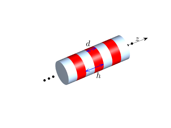
Figure 1: (Color online) Infinite circular dielectric rod with periodically alternating permittivity $\epsilon_{1}$ (dark red) and $\epsilon_{2}$ (light gray).

As shown in Fig. 1 for the stepwise behavior with $\epsilon_{2}=1$ the rod is equivalent to an one-dimensional array of dielectric discs with permittivity $\epsilon_{1}$. Irrespectively, the rod with periodically modulated permittivity preserves rotational symmetry. Each dielectric disk has two geometrical parameters, the radius $R$ and thickness $d$. That expands the domain of existence of the BSCs to substantially lower permittivities compared to the case of dielectric spheres.

II Eigenmodes with OAM $m=0$

In what follows we measure all length quantities in terms of the period $h$ of the array. Because of rotational symmetry the solutions are classified by integer $m=0,\pm 1,\pm 2,\ldots$, OAM. At first, we consider TM modes with $m=0$ and $H_{r}=0,H_{z}=0,E_{\phi}=0$ in cylindrical system of coordinates. For that case our consideration completely follows the approach by Li and Engheta for plasmonic nanowire Engheta . The solution is sought in two domains : $r<R$ and $r>R$ independently, and then matched by the continuity at the rod’s boundary $r=R$. We introduce

$$H_{\phi}(z,r)=\epsilon(z)^{1/2}\psi_{{}_{TM}}(z,r),$$

$$E_{r}=-\frac{i}{k_{0}\epsilon(z)}\frac{\partial\epsilon(z)^{1/2}\psi_{{}_{TM}}}{\partial z},$$ (1)

$$E_{z}=\frac{i}{k_{0}\epsilon(z)r}\frac{\partial\epsilon(z)^{1/2}r\psi_{{}_{TM}}}{\partial r},$$

where the function $\psi_{{}_{TM}}$ obeys equation

$$\left[\frac{\partial^{2}}{\partial r^{2}}+\frac{1}{r}\frac{\partial}{\partial r}-\frac{1}{r^{2}}+\frac{\partial^{2}}{\partial z^{2}}+U_{{}_{TM}}(z)\right]\psi_{{}_{TM}}(z,r)=0,$$ (2)

where

$$U_{{}_{TM}}(z)=\epsilon(z)k_{0}^{2}-\frac{3}{4}\left(\frac{\epsilon^{\prime}(z)}{\epsilon(z)}\right)^{2}+\frac{1}{2}\frac{\epsilon^{\prime\prime}(z)}{\epsilon(z)}.$$ (3)

For the TE mode in sector $m=0$ we have $E_{r}=E_{z}=H_{\phi}=0$ and

$$E_{\phi}=\psi_{{}_{TE}},~{}~{}H_{r}=\frac{i}{k_{0}}\frac{\partial\psi_{{}_{TE}}}{\partial z},~{}~{}H_{z}=-\frac{i}{k_{0}r}\frac{\partial r\psi_{{}_{TE}}}{\partial r}$$ (4)

where the equation for $\psi_{TE}$ has the same form as Eq. (2) except that the effective potential $U_{TM}$ is now replaced by

$$U_{TE}(z)=\epsilon(z)k_{0}^{2}.$$ (5)

Hence we can generalize Eq. (2) for both EM modes as follows

$$\left[\frac{\partial^{2}}{\partial r^{2}}+\frac{1}{r}\frac{\partial}{\partial r}-\frac{1}{r^{2}}+\frac{\partial^{2}}{\partial z^{2}}+U_{\sigma}(z)\right]\psi_{\sigma}(z,r)=0,$$ (6)

where

$$\psi_{\sigma}=\left\{\begin{array}[]{cc}E_{\phi},&\sigma=TE\\ H_{\phi}/\epsilon^{1/2},&\sigma=TM,\end{array}\right.$$ (7)

Because of periodicity of the permittivity the effective potential $U_{\sigma}(z)$ and the solution of Eq. (6) can be expanded in Bloch series as

$$U_{\sigma}(z)=k_{0}^{2}\sum_{n}U_{n}^{\sigma}e^{iqnz},q=2\pi/h,$$

$$~{}\psi_{\sigma}(z,r)=\sum_{n}\psi_{n\sigma}(r)e^{i(qn+\beta)z},$$ (8)

where $\beta$ is the Bloch vector. Then substitution of these series into Eq. (6) gives

$$\left[\frac{\partial^{2}}{\partial r^{2}}+\frac{1}{r}\frac{\partial}{\partial r}-\frac{1}{r^{2}}-(qn+\beta)^{2}\right]\psi_{n\sigma}+k_{0}^{2}\sum_{n^{\prime}}U_{n-n^{\prime}}^{\sigma}\psi_{n^{\prime}\sigma}=0.$$ (9)

The presenting the solution as Engheta

$$\psi_{\sigma}(r,z)=\sum_{sn}g_{s\sigma}c_{sn\sigma}J_{1}(\lambda_{s\sigma}r)e^{i(qn+\beta)z},$$ (10)

we rewrite Eq. (9) in the following form

$$[-\lambda^{2}_{\sigma}-(qn+\beta)^{2}]c_{n\sigma}+k_{0}^{2}\sum_{n^{\prime}}U_{n-n^{\prime}}^{\sigma}c_{n^{\prime}\sigma}=0.$$ (11)

where the eigenvalues $\lambda_{\sigma}$ and eigenvectors $\mathbf{c}_{\sigma}$ are found from the eigenvalue problem

$$\widehat{L}^{\sigma}\mathbf{c}_{\sigma}=\lambda_{\sigma}^{2}\mathbf{c}_{\sigma}$$ (12)

with the matrix

$$L_{nn^{\prime}}^{\sigma}=-(qn+\beta)^{2}\delta_{nn^{\prime}}+k_{0}^{2}U_{n-n^{\prime}}^{\sigma}.$$ (13)

Owing to the equality $\frac{d}{dx}J_{1}(x)=J_{0}(x)-\frac{1}{x}J_{1}(x)$ we have from Eq. (II) for the TM electric field inside the rod

$$E_{z}=\frac{i}{k_{0}\sqrt{\epsilon}}\sum_{sn}\lambda_{{}_{s,TM}}~{}g_{{}_{s,TM}}~{}c_{{}_{sn,TM}}J_{0}(\lambda_{{}_{s,TM}}r)e^{i(qn+\beta)z}.$$ (14)

By the use of the following series

$$\sqrt{\epsilon}=\sum_{n}a_{n}e^{iqnz},~{}~{}\frac{1}{\sqrt{\epsilon}}=\sum_{n}b_{n}e^{iqnz}$$ (15)

we obtain for the components of EM fields at $r\leq R$

$$H_{\phi}=\sum_{snl}g_{{}_{s,TM}}c_{{}_{sl,TM}}J_{1}(\lambda_{{}_{s,TM}}r)a_{n-l}e^{i(qn+\beta)z}$$

$$E_{z}=\frac{i}{k_{0}}\sum_{snl}\lambda_{{}_{s,TM}}g_{{}_{s,TM}}c_{{}_{sl,TM}}J_{0}(\lambda_{{}_{s,TM}}r)b_{n-l}e^{i(qn+\beta)z}.$$ (16)

Outside the rod we have

$$H_{\phi}=\sum_{n}h_{n}H_{1}^{(1)}(\alpha_{n}r)e^{i(qn+\beta)z},$$

$$E_{z}=\frac{i}{k_{0}}\sum_{n}\alpha_{n}h_{n}H_{0}^{(1)}(\alpha_{n}r)e^{i(qn+\beta)z},$$ (17)

where

$$\alpha_{n}=\sqrt{k_{0}^{2}-(\beta+qn)^{2}}$$ (18)

and $H_{1}^{(1)}$ and $H_{0}^{(1)}$ are the Hankel functions. Sewing at the boundary $r=R$ gives the following dispersion relation Engheta

$$Det(\widehat{S}\widehat{U}\widehat{B}-\widehat{D}\widehat{V}\widehat{T})=0$$ (19)

where the matrix elements

$$S_{nn^{\prime}}=\alpha_{n}H_{n}^{(0)}(\alpha_{n}R)\delta_{nn^{\prime}},$$

$$U_{nn^{\prime}}=a_{n-m},B_{nn^{\prime}}=c_{{}_{nn^{\prime},TM}}J_{1}(\lambda{{}_{n,TM}}R),$$

$$D_{nn^{\prime}}=H_{n}^{(1)}(\alpha_{n}R)\delta_{nn^{\prime}},V_{nn^{\prime}}=b_{n-m},$$

$$T_{nn^{\prime}}=c_{{}_{nn^{\prime},TM}}\lambda{{}_{n,TM}}J_{0}(\lambda{{}_{n,TM}}R).$$ (20)

Respectively for the TE modes we have

$$E_{\phi}=\sum_{sn}g_{{}_{s,TE}}c_{{}_{sn,TE}}J_{1}(\lambda_{{}_{n,TE}}r)e^{i(qn+\beta)z}$$

$$H_{z}=-\frac{i}{k_{0}}\sum_{sn}\lambda_{{}_{s,TE}}g_{{}_{s,TE}}c_{{}_{sn,TE}}J_{0}(\lambda_{{}_{s,TE}}r)e^{i(qn+\beta)z}.$$ (21)

Outside the rod we have

$$E_{\phi}=\sum_{n}h_{n}H_{1}^{(1)}(\alpha_{n}r)e^{i(qn+\beta)z}$$

$$H_{z}=-\frac{i}{k_{0}}\sum_{n}\alpha_{n}h_{n}H_{0}^{(1)}(\alpha_{n}r)e^{i(qn+\beta)z},$$ (22)

Repeating the above algebra for the TE mode we obtain instead of (19) the following dispersion equation

$$Det(\widehat{S}\widehat{B}-\widehat{D}\widehat{T})=0$$ (23)

where the matrix elements for all quantities have the form given by Eq. (II) with replacement $TM\rightarrow TE$.

III Sectors $m\neq 0$

Similar to the rod with the homogeneous permittivity for sectors with $m\neq 0$ the TE and TM solutions are hybridized by the boundary conditions. Let us start with pure TE mode which can be expressed through the auxiliary function $\psi_{{}_{TE}}$:

$$E_{\phi}=\frac{i}{m}\frac{\partial\psi_{TE}}{\partial r},E_{r}=\frac{\psi_{TE}}{r},$$

$$H_{\phi}=-\frac{i}{k_{0}r}\frac{\partial\psi_{TE}}{\partial z},$$

$$H_{r}=-\frac{1}{k_{0}m}\frac{\partial^{2}\psi_{TE}}{\partial z\partial r},$$

$$H_{z}=\frac{1}{k_{0}m}\left[\frac{\partial^{2}}{\partial r^{2}}+\frac{1}{r}\frac{\partial}{\partial r}-\frac{m^{2}}{r^{2}}\right]\psi_{{}_{TE}},$$ (24)

Similarly for the TM mode we have the following

$$H_{\phi}=\frac{i\sqrt{\epsilon}}{m}\frac{\partial\psi_{{}_{TM}}}{\partial r},~{}~{}H_{r}=\frac{\sqrt{\epsilon}\psi_{{}_{TM}}}{r},$$

$$E_{\phi}=\frac{i}{k_{0}\epsilon r}\frac{\partial\sqrt{\epsilon}\psi_{{}_{TM}}}{\partial z},$$

$$E_{r}=\frac{1}{k_{0}\epsilon m}\frac{\partial\sqrt{\epsilon}}{\partial z}\frac{\partial\psi_{{}_{TM}}}{\partial r},$$ (25)

$$E_{z}=-\frac{1}{k_{0}\sqrt{\epsilon}m}\left[\frac{\partial^{2}}{\partial r^{2}}+\frac{1}{r}\frac{\partial}{\partial r}-\frac{m^{2}}{r^{2}}\right]\psi_{{}_{TM}},$$

where the auxiliary functions obey the equation

$$\left[\frac{\partial^{2}}{\partial r^{2}}+\frac{1}{r}\frac{\partial}{\partial r}-\frac{m^{2}}{r^{2}}+\frac{\partial^{2}}{\partial z^{2}}+U_{\sigma}(z)\right]\psi_{\sigma}(z,r)=0.$$ (26)

The series (10) are modified as follows for both types of the modes

$$\psi_{\sigma}(r,z)=\sum_{sn}g_{s,\sigma}c_{sn\sigma}J_{m}(\lambda_{s,\sigma}r)e^{i(qn+\beta)z}.$$ (27)

Note, the eigenvalues $\lambda_{s,\sigma}$ and eigenvector amplitudes $c_{sn\sigma}$ coincide with those introduced in the previous section for $m=0$. Substituting (27) into Eq. (26) and satisfying the boundary conditions, after cumbersome algebra we obtain the following dispersion relation

$$im(\widehat{A}-i\widehat{B}-\widehat{I}\widehat{D})\overrightarrow{\psi}_{{}_{TM}}+k_{0}R(\widehat{F}-i\widehat{J}\widehat{P})\overrightarrow{\psi}_{{}_{TE}}=0,$$

$$k_{0}R(\widehat{K}-i\widehat{J}\widehat{P})\overrightarrow{\psi}_{{}_{TM}}-im\widehat{I}(\widehat{C}-\widehat{D})\overrightarrow{\psi}_{{}_{TE}}=0.$$ (28)

where according to Eq. (27) the s-th component of the vectors $\overrightarrow{\psi}_{\sigma}$ is given by

$$(\overrightarrow{\psi}_{\sigma})_{s}=g_{s,\sigma}J_{m}(\lambda_{s,\sigma}R).$$ (29)

The elements of matrices in Eq. (III) could be found as

$$A_{ns}=\sum_{l}b_{n-l}(\beta+ql)c_{sl,_{TM}},$$

$$B_{ns}=\sum_{l}d_{n-l}c_{sl,_{TM}},$$

$$I_{nm}=\delta_{nm}(\beta+qn),$$

$$J_{nm}=\delta_{nm}\alpha_{n}\frac{H_{m}^{\prime(1)}(\alpha_{n}R)}{H_{m}^{(1)}(\alpha_{n}R)},$$

$$F_{ns}=\lambda_{s,_{TE}}c_{sl,_{TE}}\frac{J_{m}^{\prime}(\lambda_{s,_{TE}}R)}{J_{m}(\lambda_{s,_{TE}}R)},$$

$$K_{ns}=\lambda_{s_{TE}}\frac{J_{m}^{\prime}(\lambda_{s_{TE}}R)}{J_{m}(\lambda_{s_{TE}}R)}\sum_{l}a_{n-l}c_{sl,_{TE}},$$

$$P_{ns}=\frac{\lambda_{s_{TE}}^{2}}{\alpha_{n}^{2}}c_{ns,_{TE}}.$$

$$D_{ns}=\frac{\lambda_{s}^{2}}{\alpha_{n}^{2}}\sum_{l}b_{n-l}c_{sl,_{TM}},$$ (30)

where

$$\frac{\epsilon^{\prime}(z)}{2\epsilon^{3/2}(z)}=\sum_{n}d_{n}e^{iqnz}.$$ (31)

In order to avoid discontinuities of the derivatives of the permittivity at the boundary of the disc $z=\pm 1/2$ we following Ref. Engheta smooth the boundary by the function

$$\epsilon(z)=\epsilon_{2}+\frac{1}{2}(\epsilon_{1}-\epsilon_{2})[1-\tanh(\kappa(|z|-1/2))]$$

with the control parameter $\kappa$. In what follows we take $\kappa=17$.

IV Symmetry classification of BSCs

Similar to the periodic array of dielectric spheres the BSCs in the single rod with periodically modulated permittivity are classified by the OAM $m$ due to the rotational symmetry of the rod and the Bloch vector along the rod due to the translational symmetry. Moreover there is the mirror symmetry $z\rightarrow-z$. That allows us to classify the BSCs with $\beta=0$ by parity. These standing wave BSCs are symmetry protected relative to ever the TE diffraction continuum or the TM continuum. Introduce the operator $\widehat{O}f(z)=f(-z)$. Respectively after the Fourier transformation we have $\widehat{O}f_{n}=f_{-n}$ and therefore $O_{nn^{\prime}}=\delta_{n+n^{\prime},0}$. The operator $\widehat{L}^{\sigma}$ with matrix elements given by Eq. (13) for $\beta=0$ commutes with the operator $\widehat{O}$. Therefore the eigenvectors of the operator $\widehat{L}^{\sigma}$ are classified as even and odd

$$c_{sn,\sigma}=\pm c_{s,-n,\sigma}.$$ (32)

Let us rewrite Eq. (III) as follows

$$\widehat{H}_{{}_{1,TM}}\overrightarrow{\psi}_{{}_{TM}}+\widehat{H}_{{}_{1,TE}}\overrightarrow{\psi}_{{}_{TE}}=0,$$

$$\widehat{H}_{{}_{2,TM}}\overrightarrow{\psi}_{{}_{TM}}+\widehat{H}_{{}_{2,TE}}\overrightarrow{\psi}_{{}_{TE}}=0,$$ (33)

where matrices $\widehat{H}_{k,\sigma},k=1,2$ are of the size $(2N+1)\times(2N+1)$. We arrange the matrices as follows

$$\widehat{H}_{{}_{1,TE}}=[\widehat{H}_{{}_{1,TE}}^{e}\{(2N+1)\times(N+1)\},~{}~{}\widehat{H}_{{}_{1,TE}}^{o}\{(2N+1)\times N\}],$$

$$\widehat{H}_{{}_{1,TM}}=[\widehat{H}_{{}_{1,TM}}^{e}\{(2N+1)\times N\},~{}~{}\widehat{H}_{{}_{1,TM}}^{o}\{(2N+1)\times(N+1)\}],$$

$$\widehat{H}_{{}_{2,TE}}=[\widehat{H}_{{}_{2,TE}}^{o}\{(2N+1)\times(N+1)\},~{}~{}\widehat{H}_{{}_{2,TE}}^{e}\{(2N+1)\times N\}],$$ (34)

$$\widehat{H}_{{}_{2,TM}}=[\widehat{H}_{{}_{2,TM}}^{o}\{(2N+1)\times N\},~{}~{}\widehat{H}_{{}_{2,TM}}^{e}\{(2N+1)\times(N+1)\}]$$

where expressions in curly brackets show the size of the matrices and the matrix elements are even or odd relative to $n\rightarrow-n$:

$$\widehat{H}_{nn^{\prime},\sigma}^{e}=\widehat{H}_{-nn^{\prime},\sigma}^{e},~{}~{}\widehat{H}_{nn^{\prime},\sigma}^{o}=-\widehat{H}_{-nn^{\prime},\sigma}^{o}.$$ (35)

Substituting relations (IV) into Eq. (IV) and splitting the vector

$$\overrightarrow{\psi}_{{}_{TE}}=\left(\begin{array}[]{c}\overrightarrow{\psi}_{\uparrow_{TE}}\{N+1\}\\ \overrightarrow{\psi}_{\downarrow_{TE}}\{N\}\\ \end{array}\right),~{}~{}\overrightarrow{\psi}_{{}_{TM}}=\left(\begin{array}[]{c}\overrightarrow{\psi}_{\uparrow_{TM}}\{N\}\\ \overrightarrow{\psi}_{\downarrow_{TM}}\{N+1\}\\ \end{array}\right),$$

we obtain the following equations

$$\widehat{H}_{{}_{1,TM}}^{e}\overrightarrow{\psi}_{\uparrow_{TM}}+\widehat{H}_{{}_{1,TM}}^{o}\overrightarrow{\psi}_{\downarrow_{TM}}+\widehat{H}_{{}_{1,TE}}^{e}\overrightarrow{\psi}_{\uparrow_{TE}}+\widehat{H}_{{}_{1,TE}}^{o}\overrightarrow{\psi}_{\downarrow_{TE}}=0,$$

$$\widehat{H}_{{}_{2,TM}}^{o}\overrightarrow{\psi}_{\uparrow_{TM}}+\widehat{H}_{{}_{2,TM}}^{e}\overrightarrow{\psi}_{\downarrow_{TM}}+\widehat{H}_{{}_{2,TE}}^{o}\overrightarrow{\psi}_{\uparrow_{TE}}+\widehat{H}_{{}_{2,TE}}^{e}\overrightarrow{\psi}_{\downarrow_{TE}}=0.$$ (36)

From Eqs. (35) and (IV) it follows that there are two solutions. The first is $\overrightarrow{\psi}_{\downarrow\sigma}=0$ and $\overrightarrow{\psi}_{\uparrow\sigma}\neq 0$ with $H_{z},E_{\phi}$, and $E_{r}$ even and $E_{z},H_{\phi}$ and $H_{r}$ odd relative to the inversion $z\rightarrow-z$. This solution gives us a TM symmetry protected BSC. The second solution $\overrightarrow{\psi}_{\uparrow\sigma}=0$ and $\overrightarrow{\psi}_{\downarrow\sigma}\neq 0$ has odd field components $H_{z},E_{\phi}$, and $E_{r}$ even $E_{z},H_{\phi}$ and $H_{r}$. This solution is a TE symmetry protected BSC. By solving Eqs. (19), (23) and (III) numerically we obtain the following set of BSCs. In particular there are symmetry protected BSCs with definite polarization which occur at arbitrary radius of the rod:

(1) Symmetry protected TE BSCs with $\beta=0,m=0$ and $H_{z}(-z)=-H_{z}(-z)$.

(2) Symmetry protected TM BSCs with $\beta=0,m=0$ and $E_{z}(-z)=-E_{z}(-z)$.

Examples of these symmetry protected BSCs are shown in Fig. 2 and Fig. 3.

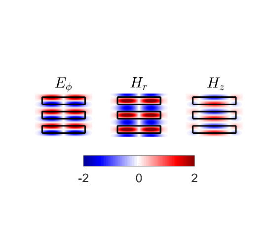
Figure 2: Pattern of the symmetry protected TE BSC with zero OAM $m=0$, frequency $k_{0c}=4.6063$ and $\beta=0$ for parameters: $\epsilon_{1}=3,\epsilon_{2}=1,R=1.5,d=0.5$.

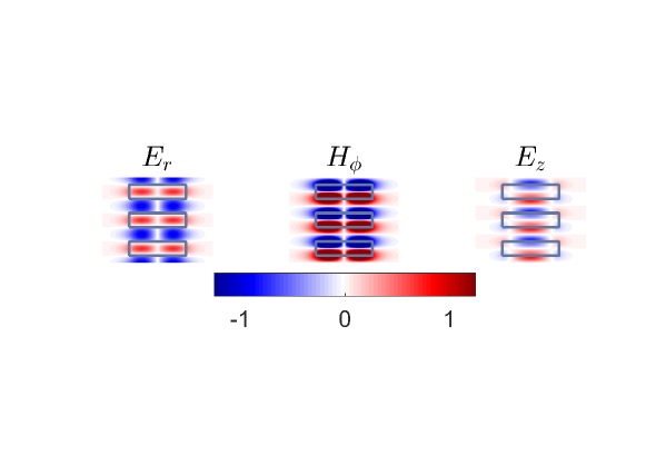
Figure 3: Pattern of the symmetry protected TM BSC with zero OAM $m=0$, frequency $k_{0c}=5.37652$ and $\beta=0$ for parameters: $\epsilon_{1}=3,\epsilon_{2}=1,R=1,d=0.5$.

The next class of the BSCs with definite polarization are non-symmetry protected and require tuning the rod radius $R$:

(3) Non-symmetry protected TE BSCs with $\beta=0,m=0$ and $H_{z}(-z)=H_{z}(-z)$.

(4) Non-symmetry protected TM BSCs with $\beta=0,m=0$ and $E_{z}(-z)=E_{z}(-z)$.

These BSCs are shown in Fig. 4 and Fig. 5.

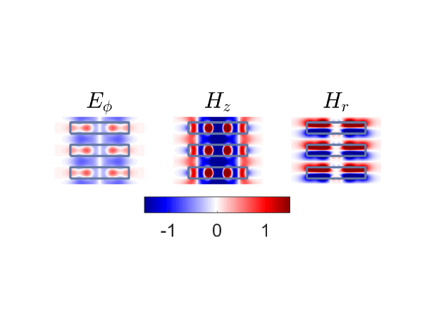
Figure 4: Pattern of the non symmetry protected TE BSC with $m=0,\beta=0$ and frequency $k_{0c}=4.63778$ for parameters: $\epsilon_{1}=5,\epsilon_{1}=1,R=1.3061,d=0.5$.

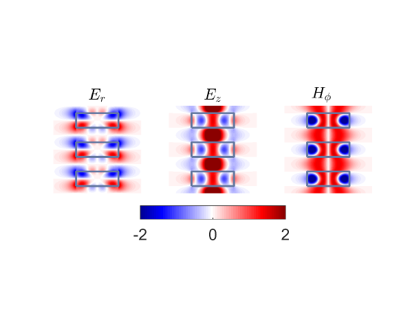
Figure 5: Pattern of the non symmetry protected TM BSC with $m=0,\beta=0$ and frequency $k_{0c}=4.85502$ for parameters: $\epsilon_{1}=5,\epsilon_{2}=1,R=0.724504,d=0.5$.

(5) Bloch BSCs with $\beta\neq 0,m=0$ with definite polarization shown in Fig. 6 and Fig. 7. They exist within a wide interval of the rod radius. Rigorously speaking the Bloch BSCs can not be considered as guided modes similar to those which exist below light line in the homogeneous dielectric rod Jackson . However those Bloch quasi-BSCs in some small interval of $\beta$ around the BSC point have the lifetimes exceeding the propagation time in the rod of finite length and thus can be considered as the guided modes above the light line OL .

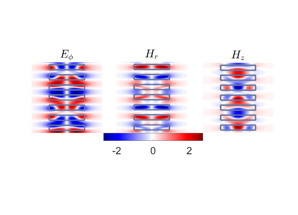
Figure 6: (Color online) Pattern of the Bloch TE BSC with $m=0,\beta_{c}=2.37361$ and frequency $k_{0c}=3.15725$ for parameters: $\epsilon_{1}=5,R=1,d=0.5$.

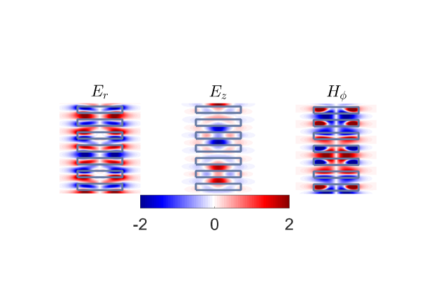
Figure 7: (Color online) Pattern of the Bloch TM BSC with $m=0,\beta_{c}=1.08676$ and frequency $k_{0c}=3.88423$ for parameters: $\epsilon_{1}=5,R=1,d=0.5$.

(6) BSCs with orbital angular momentum (OAM) $m\neq 0$ and $\beta=0$ constitute the most interesting class. Whilst in the array of spheres we managed to find only BSCs with $m=1$ and $m=2$ PRA94 ; Adv EM . In the array of discs we found BSCs with higher OAM. However, in contrast to the array of spheres we did not find any Bloch BSCs with $m\neq 0$ and $\beta\neq 0$. The BSCs with OAM are hybridized with respect to polarization. They are symmetry protected against decay into the TE/TM continuum as it was considered above but the radius has to be tuned for the mode be decoupled from the TM/TE continuum. Figs. 8–11 show the solutions of Eq. (III) for BSCs with $m=1,2,5,10$, and $\beta=0$. All BSCs with nonzero OAM were calculated for $\epsilon_{1}=3,\epsilon_{2}=1$ and $d=0.5$.

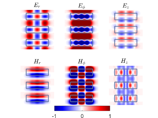
Figure 8: (Color online) Pattern of the BSC with $m=1$ symmetry protected in respect to the TM radiation continuum and frequency $k_{0c}=5.26284$ for tuned radius $R=1.65293$.

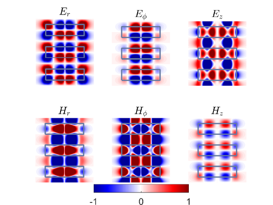
Figure 9: (Color online) Pattern of the BSC with $m=2$ symmetry protected in respect to the TE radiation continuum and frequency $k_{0c}=5.21418$ for tuned radius $R=1.7009$.

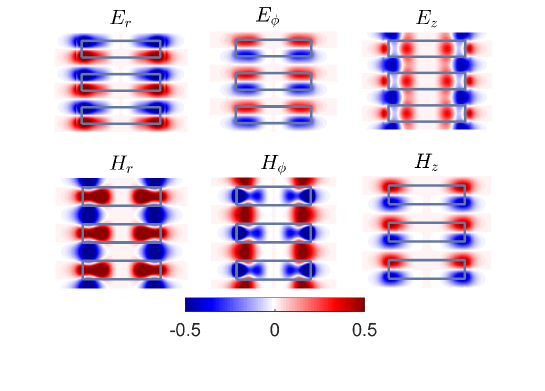
Figure 10: (Color online) Pattern of the BSC with $m=5$ symmetry protected in respect to the TE radiation continuum and frequency $k_{0c}=5.14387$ for tuned radius $R=1.87591$.

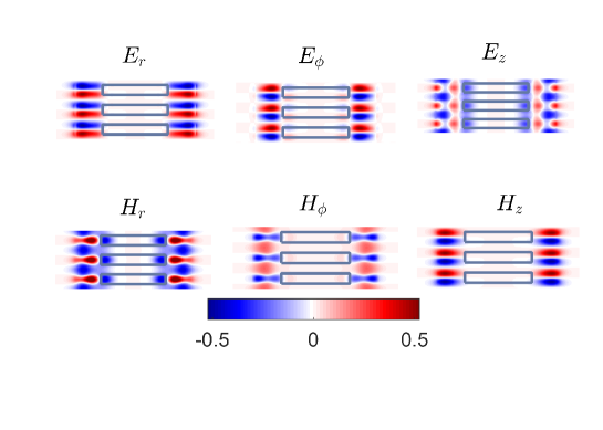
Figure 11: (Color online) Pattern of the BSC with $m=10$ symmetry protected in respect to the TE radiation continuum and frequency $k_{0c}=5.29052$ for tuned radius $R=3.07046$.

One can see from Figs. 10 and 11 a tendency of light localization at the surface of the rod with growth of the OAM $m$ limiting to whispering gallery modes. However, in contrast to the latter the BSCs with OAM exist for any $m$.

The BSC with OAM is degenerate with respect to the sign of $m$. The sign controls the direction of spinning of the Poynting vector $\overrightarrow{j}=j_{0}\overrightarrow{E}\times\overrightarrow{H}$ as demonstrated in Fig. 12. We mention in passing that the spinning trapped modes in an acoustic cylindrical infinitely long waveguide which contains rows of large numbers of blades arranged around a central core was first reported by Duan and McIver Duan .

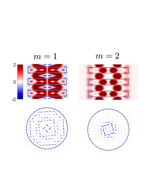
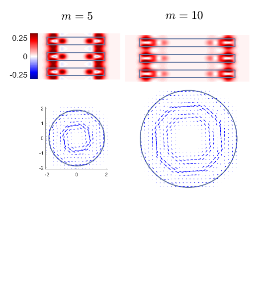
Figure 12: (Color online) The profile $H_{z}$ and flows of Pointing vector at $z=0$ circulating around core of the rod in the BSCs shown in Fig. 11.

V Limits of the BSCs for $d\rightarrow 1$ and $d\ll 1$

Until now we considered trapping of light by a stack of dielectric discs whose thickness equals half of the period. In this section we consider what happens with the BSC when the rod becomes homogeneous and when the discs become veru thin.

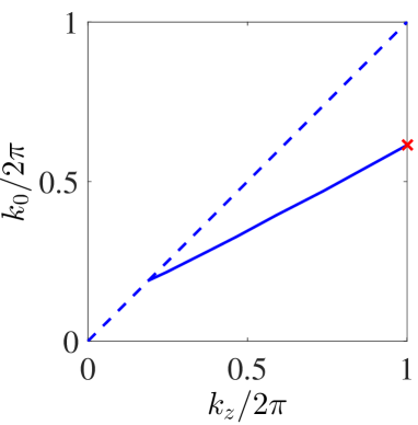
Figure 13: Dispersion curve of the waveguide mode, bound state below the light line in the homogeneous rod with the radius $R=1.5$ and permittivity $\epsilon_{1}=3$.

The homogeneous rod which can support only guided modes with $k_{z}>0$ below the light line. In the latter the Maxwell equations can be solved by separation of variables for the TE polarization with zero OAM $m=0$ Jackson

$$H_{z}(r,z)=\left\{\begin{array}[]{cc}e^{ik_{z}z}J_{0}(\sqrt{\epsilon k_{0}^{2}-k_{z}^{2}}r)&r\leq R,\\ Ae^{ik_{z}z}K_{0}(\sqrt{k_{z}^{2}-k_{0}^{2}}r)=\frac{i\pi A}{2}e^{ik_{z}z}H_{0}^{(1)}(\sqrt{k_{0}^{2}-k_{z}^{2}}r)&r>R,\end{array}\right.$$ (37)

to result in guided mode, bound state below the light line $k_{z}<k_{0}$ after matching at $r=R$. Numerical result for the dispersion curve of the lowest TE mode in the homogeneous cylindrical rod is shown in Fig. 13 where the frequency of this solution $k_{0}=3.858$ at $k_{z}=2\pi$ is marked by cross.

As soon as the rod acquires a periodic modulation of the permittivity $\epsilon(z)=\epsilon(z+l),~{}~{}l=0,\pm 1,\pm 2,\ldots$ the radiation continua in the form of the Hankel functions (37) is quantized $k_{z,n}=\beta+2\pi n$. In the other words, the rod can be viewed as one-dimensional cylindrical diffraction lattice Ndangali2010 ; PRA92 . Let us consider the TE BSC symmetry protected against the lowest diffraction continuum $n=0$ above light line shown by dash line in Fig. 13. Its solution takes the following form for $r>R$

$$H_{z}(r,z)=-\frac{i}{k_{0}}\sum_{n}h_{n}\alpha_{n}H_{0}^{(1)}(\alpha_{n}r)\sin(2\pi nz)$$ (38)

where $a_{n}$ are given by Eq. (18). In particular this solution turns to the symmetry protected TE BSC shown in Fig. 2 if all $h_{n}=0$ except $h_{1}$. The dependence of the BSC frequency on the disc thickness is shown in Fig. 14 which limits to the value $k_{0c}=3.858$ which is just the the frequency of the solution of the homogeneous rod (37) marked by cross in Figs. 13 and 14. The solution is very similar to that shown in Fig. 2 but is more localized.

In the second limit when the disk thickness $d$ decreases the mean permittivity of the rod drops as well and respectively the BSC frequency grows as plotted in Fig. 14.

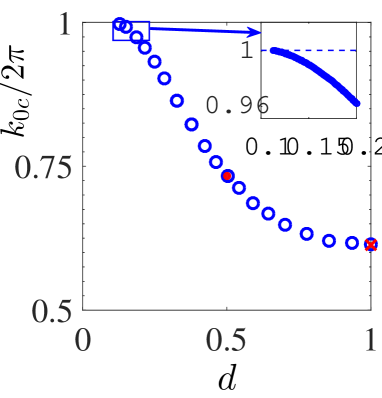
Figure 14: Frequency of the TE symmetry protected BSC vs the thickness of discs in terms of the period $h$ for $R=1.5$. Closed circle notes the BSC shown in Fig. 2 for $d=0.5$.

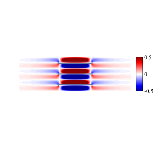
Figure 15: Pattern of the TE symmetry protected BSC at $d=0.132,R=1.5$.

The further decrease of the thickness $d$ brings the BSC frequency to the bottom of the second diffraction continuum $2\pi$ where the BSC is corrupted by leakage into that continuum. In the zoomed window in Fig. 14 we show it occurs at $d=0.112$ for $\epsilon_{1}=3$. Thus the thickness of disks is limited for the TE symmetry protected BSC to exist. The radius of localization of the BSC behaves as

$$R_{c}\approx\frac{1}{\sqrt{4\pi^{2}-{k_{0c}^{2}}}}.$$ (39)

Fig. 15 illustrates the $H_{z}$ component of the BSC solution near the bottom of the second diffraction continuum at $d=0.137$. One can see that the radius of localization is tremendously increased compared to the case $d=0.5$ shown in Fig. 2. According to Eq. (39) the radius of localization of the BSC goes to infinity when $d\rightarrow 0.112$.

VI Summary

We considered light trapping in a single infinitely long dielectric rod with periodically modulated permittivity. We restrict ourselves with stepwise behavior of the permittivity intermittently changing from $\epsilon_{2}=1$ to $\epsilon_{1}>1$ to makes the rod equivalent to a stack of dielectric discs. Even in that particular case owing to the possibility of tuning two dimensional parameters, the radius and thickness of the discs and the permittivity we have an abundance of BSCs compared to the array of dielectric spheres Adv EM . The stack of discs preserves the rotational symmetry to give rise to BSCs with definite OAM. However, in contrast to the array of spheres the rod with periodically modulated permittivity supports BSCs with OAM up to $m=10$ for a sufficiently large radius as shown in Fig. 10. We also found Bloch BSCs with both polarizations however, only with zero OAM. Bloch BSCs with non zero OAM have not been found yet.

In the limit $d\rightarrow 1$ when the discs mold into single homogeneous rod we have shown that the symmetry protected BSC with $m=0$ transforms into the guided mode below the light line. In the limit of thin discs $d\ll 1$ the BSC frequency reaches the bottom of the second diffraction continuum and is destroyed by leakage into that continuum. The problem of BSCs can be also solved for sinusoidal behavior $\epsilon(z)=\epsilon_{0}+\lambda\sin 2\pi z$.

Acknowledgments: We acknowledge discussions with D.N. Maksimov and A.S. Aleksandrovsky. This work was partially supported by Ministry of Education and Science of Russian Federation (State contract N 3.1845.2017) and RFBR grant 16-02-00314.

References

- (1) A.-S. Bonnet-Bendhia and F. Starling, ”Guided waves by electromagnetic gratings and non uniqueness examples for the diffraction problem,” Math. Methods Appl. Sci. 17, 305 (1994).
- (2) S. Shipman and S. Venakides, ”Resonance and bound states in photonic crystal slabs”, SIAM J. Appl. Math. 64, 322 (2003).
- (3) S.P. Shipman and S. Venakides, ”Resonant transmission near non robust periodic slab modes”, Phys. Rev. E71, 026611 (2005).
- (4) D. C. Marinica, A. G. Borisov, and S.V. Shabanov, ”Bound States in the Continuum in Photonics”, Phys. Rev. Lett. 100, 183902 (2008).
- (5) R.F. Ndangali and S.V. Shabanov, ”Electromagnetic bound states in the radiation continuum for periodic double arrays of subwavelength dielectric cylinders”, J. Math. Phys. 51, 102901 (2010).
- (6) Chia Wei Hsu, Bo Zhen, J. Lee, Song-Liang Chua, S.G. Johnson, J.D. Joannopoulos, and M. Soljačić, ”Observation of trapped light within the radiation continuum, Nature, 499, 188 (2013).
- (7) S. Weimann, Yi Xu, R. Keil, A.E. Miroshnichenko, A. Tunnermann, S. Nolte, A.A. Sukhorukov, A. Szameit, and Yu.S. Kivshar, ”ompact Surface Fano States Embedded in the Continuum of Waveguide Arrays”, Phys. Rev. Lett. 111, 240403 (2013).
- (8) Chia Wei Hsu, Bo Zhen, Song-Liang Chua, S.G. Johnson, J.D.Joannopoulos, and M. Soljačić, ”Bloch surface eigen states with in the radiation continuum”, Light: Science and Applications 2, 1 (2013).
- (9) Bo Zhen, Chia Wei Hsu, Ling Lu, A.D. Stone, and M. Soljačić, ”Topological Nature of Optical Bound States in the Continuum”, Phys. Rev. Lett. 113, 257401 (2014).
- (10) Yi Yang, Chao Peng, Yong Liang, Zhengbin Li, and S. Noda, ”Analytical Perspective for Bound States in the Continuum in Photonic Crystal Slabs”, Phys.Rev. Lett. 113, 037401 (2014).
- (11) E.N. Bulgakov and A.F. Sadreev, ”Bloch bound states in the radiation continuum in a periodic array of dielectric rods”, Phys. Rev. A90, 053801 (2014).
- (12) J.M. Foley, S.M. Young, and J.D. Phillips, ”Symmetry-protected mode coupling near normal incidence for narrow-band transmission filtering in a dielectric grating”, Phys. Rev. B 89, 165111 (2014).
- (13) Zhen Hu and Ya Yan Lu, ”Standing waves on two-dimensional periodic dielectric waveguides”, J. Optics, 17, 065601 (2015).
- (14) Maowen Song, Honglin Yu, Changtao Wang, Na Yao, Mingbo Pu, Jun Luo, Zuojun Zhang, and Xiangang Luo, ”Sharp Fano resonance induced by a single layer of nanorods with perturbed periodicity”, Opt. Express, 23, 2895-2903 (2015).
- (15) Chang-Ling Zou, Jin-Ming Cui, Fang-Wen Sun, Xiao Xiong, Xu-Bo Zou, Zheng-Fu Han, and Guang-Can Guo, ”Guiding light through optical bound states in the continuum for ultrahigh-Q microresonators”, Laser Photonics Rev. 9, 114 119 (2015).
- (16) Lijun Yuan and Ya Yan Lu, ”Diffraction of plane waves by a periodic array of nonlinear circular cylinders,” Phys. Rev. A 94, 013852 (2016).
- (17) Zhixin Wang, Hanxing Zhang, Liangfu Ni, Weiwei Hu, and Chao Peng, ”Analytical Perspective of Interfering Resonances in High-Index-Contrast Periodic Photonic Structures”, IEEE J. Quant. Electr. 52, 6100109 (2016).
- (18) Lijun Yuan and Ya Yan Lu, ”Propagating Bloch modes above the lightline on a periodic array of cylinders”, J. Phys. B: At. Mol Phys.
- (19) Z.F. Sadrieva, I.S Sinev, K.L. Koshelev, A. Samusev, I.V. Iorsh, O. Takayama, R. Malureanu, A.A. Bogdanov, and A.V. Lavrinenko, ”Transition from optical bound states in the continuum to leaky resonances: role of substrate and roughness,” ACS Photonics (2017).
- (20) J. Lee, B. Zhen, S.-L. Chua, W. Qiu, J.D. Joannopoulos, M. Soljačić, and O. Shapira, ”Observation and Differentiation of Unique High-Q Optical Resonances Near Zero Wave Vector in Macroscopic Photonic Crystal Slabs,” Phys. Rev. Lett., 109, 067401 (2012).
- (21) Yifei Wang, Jiming Song, Liang Dong, and Meng Lu, ”Optical bound states in slotted high-contrast gratings”, J. Opt. Soc. Am. B 33, 2472 (2016).
- (22) Jae Woong Yoon, Seok Ho Song and R. Magnusson, ”Critical field enhancement of asymptotic optical bound states in the continuum”, Sc. Rep. 5:18301 (2016).
- (23) Xingwei Gao, Chia Wei Hsu, Bo Zhen, Xiao Lin, J.D. Joannopoulos, M. Soljačić and Hongsheng Chen, ”Formation mechanism of guided resonances and bound states in the continuum in photonic crystal slabs”, Sc. Rep. 6:31908 (2016).
- (24) C. Blanchard, J.-P. Hugonin, and C. Sauvan, ”Fano resonances in photonic crystal slabs near optical bound states in the continuum”, Phys. Rev. B 94, 155303 (2016).
- (25) Mingda Zhang and Xiangdong Zhang, ”Ultrasensitive optical absorption in graphene based on bound states in the continuum”, Sc. Rep. 5: 8266 (2015).
- (26) A. Kodigala, T. Lepetit, Qing Gu, B. Bahari, Y. Fainman and B. Kanté, ”Lasing action from photonic bound states in continuum”, Nature, 541, 196 (2017).
- (27) L. Li and H. Yin, ”Bound States in the Continuum in double layer structures”, Scientific Reports 6 26988 (2016).
- (28) E.N. Bulgakov and A.F. Sadreev, Light trapping above the light cone in one-dimensional array of dielectric spheres, Phys. Rev. A 92 023816 (2015).
- (29) E.N. Bulgakov and A.F. Sadreev, ”Transfer of spin angular momentum of an incident wave into orbital angular momentum of the bound states in the continuum in an array of dielectric spheres, Phys. Rev. A 94 033856 (2016).
- (30) E.N. Bulgakov and D.N. Maksimov, Light guiding above the light line in arrays of dielectric nanospheres , Opt.Lett. 41, 3888 (2016).
- (31) E.N. Bulgakov, A.F. Sadreev, and D.N. Maksimov, ”Light Trapping above the Light Cone in One-Dimensional Arrays of Dielectric Spheres” (Review), Appl. Science 7, 147 (2017).
- (32) E.N. Bulgakov and A.F. Sadreev, ”Propagating Bloch bound states with orbital angular momentum above the light line in the array of dielectric spheres”, to be published in J. Opt. Soc. Am.
- (33) E.N. Bulgakov and A.F. Sadreev, ”Trapping of light with angular orbital momentum above the light cone in a periodic array of dielectric spheres”, Adv. EM, 6, 1 (2017).
- (34) Liangfu Ni, Jicheng Jin, Chao Peng, ”Analytical and statistical investigation on structural fluctuations induced radiation in photonic crystal slabs”, Opt. Express,25, 5580 (2017).
- (35) J. Li and N. Engheta, ” Subwavelength plasmonic cavity resonator on a nanowire with periodic permittivity variation”, Phys. Rev. B 74, 115125 (2006).
- (36) J. D. Jackson, Classical Electrodynamics (John Wiley and Sons, Inc., New York, 1962).
- (37) J. A. Stratton, Electromagnetic Theory, ( McGraw-Hill, New York) (1941).
- (38) A.F. Sadreev, E.N. Bulgakov, and I. Rotter, Phys. Rev. B 73, 235342 (2006).
- (39) M. Büttiker, Y. Imry, and R. Landauer, Phys. Lett. A 96, 365 (1983).
- (40) Y. Duan and M. McIver, ”Rotational acoustic resonances in cylindrical waveguides”, Wave Motion, 39(3), 261–274 (2004).
- (41) V.A. Sablikov, A.A. Sukhanov, Phys. Lett. A 379, 1775 (2015).
- (42) E.N. Bulgakov and A.F. Sadreev, ”Bound states in the continuum in photonic waveguides inspired by defects”, Phys. Rev. B78, 075105 (2008).
- (43) M. López-García, J.F. Galisteo-López, C. López, and A. García-Martín, ”Light confinement by two-dimensional arrays of dielectric spheres”, Phys. Rev. B85, 235145 (2012).