Integral points on Markoff type cubic surfaces

Abstract.

For integers $k$, we consider the affine cubic surface $V_{k}$ given by $M({\bf x})=x_{1}^{2}+x_{2}^{2}+x_{3}^{2}-x_{1}x_{2}x_{3}=k$. We show that for almost all $k$ the Hasse Principle holds, namely that $V_{k}(\mathbb{Z})$ is non-empty if $V_{k}(\mathbb{Z}_{p})$ is non-empty for all primes $p$, and that there are infinitely many $k$’s for which it fails. The Markoff morphisms act on $V_{k}(\mathbb{Z})$ with finitely many orbits and a numerical study points to some basic conjectures about these “class numbers” and Hasse failures. Some of the analysis may be extended to less special affine cubic surfaces.

1. Introduction

Little is known about the values at integers assumed by affine cubic forms $F$ in three variables. Unless otherwise stated, by an affine form $f$ in $n$-variables we mean $f\in\mathbb{Z}[x_{1},\ldots,x_{n}]$ whose leading homogeneous term $f_{0}$ is non-degenerate and such that $f-k$ is (absolutely) irreducible for all constants $k$. For $k\in\mathbb{Z}$ set

(1.1) $$V_{k,F}=\{{\bf x}=(x_{1},x_{2},x_{3}):\ F({\bf x})=k\},$$

and $\mathfrak{v}_{F}(k):=|V_{k,F}(\mathbb{Z})|$. The basic question is for which $k$ is $V_{k,F}(\mathbb{Z})\neq\emptyset$, or more generally infinite or Zariski dense in $V_{k,F}$ ?

A prime example is $F=S$, the sum of three cubes:

(1.2) $$S(x_{1},x_{2},x_{3})=x_{1}^{3}+x_{2}^{3}+x_{3}^{3}.$$

There are obvious local congruence obstructions, namely that $V_{k,S}(\mathbb{Z})=\emptyset$ if $k\equiv 4\ \text{or}\ 5\,({\rm mod}\,9)$, but beyond that it is possible that the answers to all three questions is yes for all the other $k$’s, which we call the admissible values (see [Mor69], [CV94]). It is known that strong approximation in its strongest form fails for $V_{k,S}(\mathbb{Z})$; the global obstruction coming from an application of cubic reciprocity ([Cas85], [HB92], [CTW12]). Moreover, [Leh56] and [Beu95] show that $V_{1,S}(\mathbb{Z})$ is Zariski dense in $V_{1,S}$.

The case when the cubic polynomial $F(x_{1},x_{2},x_{3})$ factors into linear factors can be studied algebraically using divisor theory, and is apparently quite different to our irreducible $F$. If $F$ is the split norm form $N({\bf x})=x_{1}x_{2}x_{3}$, then every $V_{k,N}$ is non-empty, and for $k$ non-zero, $\mathfrak{v}_{N}(k)$ is finite and is a divisor function.

For a $\mathbb{Q}$-anistropic torus given by $N({\bf x})={Nm}_{K/\mathbb{Q}}(\alpha_{1}x_{1}+\alpha_{2}x_{2}+\alpha_{3}x_{3})$, where $\alpha_{1},\,\alpha_{2},\,\alpha_{3}$ is a $\mathbb{Z}$-basis of an order in a cubic number field $K$, the Dirichlet Unit Theorem coupled with the action ${\bf w}\rightarrow u{\bf w}$ of the unit group on the homogeneous space and the theory of divisors, allows for the study of $V_{k,N}({\mathbb{Z}})$. It consists of a finite number $\mathfrak{h}_{N}(k)$ of orbits (putting $\mathfrak{h}_{N}(k)=\mathfrak{v}_{N}(k)=0$ if $V_{k,N}=\emptyset$), is infinite if it is non-empty and is Zariski dense if $K$ is totally real. The dependence of $\mathfrak{h}_{N}(k)$ on $k$ is subtle, especially if the class number $H$ of the order is not one. Most $k$’s are not represented; in fact [Odo77] shows that

(1.3) $$\big{|}\{|k|\leq X:\mathfrak{v}_{N}(k)\neq 0\}\big{|}\sim\frac{1}{H}\big{|}\{|k|\leq X:k\ \text{admissible}\}\big{|}\sim CX(\log X)^{-\frac{2}{3}}\,,$$

as $X\to\infty$ . The question of the density of Hasse failures for norms of elements in a number field $K$ is studied in [BN16].

To measure the richness of representations by $f$, we say that $f$ is perfect if $V_{k,f}(\mathbb{Z})$ is Zariski dense in $V_{k,f}$ for all but finitely many admissible $k$’s; we say it is almost perfect if the same holds for almost all admissible $k$ (in the sense of natural density); and $f$ is full if $\mathfrak{v}_{f}(k)\to\infty$ as $k\to\infty$ for almost all admissible $k$’s. For an affine form, it follows from [LW54] and [Sch76] that the admissible $k$’s are given in terms of a congruence condition as in the case of $S$.

Much more is known about cubic forms in the “subcritical” case of forms in four or more variables or diagonal forms $f=x_{1}^{a_{1}}+\ldots+x_{b}^{a_{b}}$ with $\sum_{j=1}^{b}a_{j}^{-1}>1$ and $b\geq 3$ (see [Hoo16], [VW02], [Bro15] for example) and in the “super-critical" case of two variables ([FZ14]). The basic analytic feature in the subcritical case is that the average number of representations of $k$ is $k^{\delta}(\log k)^{A}$ for some $\delta>0$, while in the critical case, $\delta=0$. If $f$ is a cubic polynomial, $n\geq 10$ and $f_{0}$ is nonsingular then $f$ is perfect ([BHB09]). In a recent paper [Hoo16], it is shown that if $f=f_{0}$ and is nonsingular with $n\geq 5$, then $f$ is full, while conditional on the Riemann Hypothesis for certain Hasse-Weil $L$-functions, the same is true for $n\geq 4$. Moreover, it is conjectured there that any such $f$ with $n\geq 4$ is perfect. For cubic $f$ in two variables (supercritical case) the celebrated theorems ([Thu09], [Sie29]) assert that $V_{k,f}(\mathbb{Z})$ is finite and moreover only for very few of the admissible $k$’s is $V_{k,f}(\mathbb{Z})$ non-empty ([Sch87]).

Returning to the critical dimension $n=3$ for affine cubic forms, there are well-known examples of $F$ which are not perfect, see ([Mor53], [CG66]) and also our example of $M$ below; however it is possible that $F$ is always full (see the discussion at the end of the Introduction).

This paper is concerned with $F=M$ where

(1.4) $$M({\bf x})=x_{1}^{2}+x_{2}^{2}+x_{3}^{2}-x_{1}x_{2}x_{3}.$$

The affine cubic surface $V_{0,M}(\mathbb{Z})$ was studied by Markoff ([Mar79], [Mar80]); the points $(x_{1},x_{2},x_{3})\in V_{0,M}(\mathbb{Z})$ with $x_{j}\in\mathbb{N}$ being essentially the “Markoff triples” . The reason that one can study $V_{0,M}(\mathbb{Z})$, or more generally $V_{k,M}(\mathbb{Z})$ is that there is a descent group action albeit non-linear. The Vieta involutions $\mathcal{V}_{j}$ with $\mathcal{V}_{1}(x_{1},x_{2},x_{3})=(x_{2}x_{3}-x_{1},x_{2},x_{3})$ and similarly for $\mathcal{V}_{2}$, $\mathcal{V}_{3}$, preserve $M$, as do permutations of the $x_{j}$’s and switching the signs of two of the $x_{j}$’s. We denote by $\Gamma$ the group of polynomial affine transformations generated as above. Then, $\Gamma$ preserves $V_{k,M}(\mathbb{Z})$ and except for the case of the Cayley cubic with $k=4$ (see Sec. 4.3), $V_{k,M}(\mathbb{Z})$ decomposes into a finite number $\mathfrak{h}_{M}(k)$ of $\Gamma$-orbits. For example, if $k=0$, then $\mathfrak{h}_{M}(0)=2$ corresponds to the orbits of $(0,0,0)$ and $(3,3,3)$ ([Mar80]). If $V_{k,M}(\mathbb{Z})\neq\emptyset$ (so that $\mathfrak{h}_{M}(k)>0$) and $k\geq 5$ or $k<0$ with $k$ not a square, which will be our cases of interest, then each $\Gamma$-orbit is infinite and even Zariski dense in $V_{k,M}$ (see [CZ06], [CL09] and Sec. 5). In particular, for $k\geq 5$ and $k$ not a square, or $k\leq 0$

(1.5) $$V_{k,M}(\mathbb{Z})\neq\emptyset\quad\text{iff}\quad V_{k,M}(\mathbb{Z})\text{ is Zariski dense in}\ V_{k,M}.$$

Moreover, $V_{k,M}(\mathbb{Z})$ contains polynomial parametric solutions $\left(x_{1}(m),x_{2}(m),x_{3}(m)\right)$ if and only if $k=4+\nu^{2}$, in which case it contains a line (see Sec. 5 for a direct proof). In [BGS16b] and [BGS16a], it is shown that these affine cubic surfaces with $V_{k,M}(\mathbb{Z})\neq\emptyset$ satisfy a form of strong approximation, after taking into account the possible finite orbits of $\Gamma$ in $V_{k,M}(\bar{\mathbb{Q}})$. Our goal in this paper is to study the set of $k$’s for which $\mathfrak{h}_{M}(k)>0$.

The first issue is to determine the congruence obstructions for $k$. This is elementary and in Section 6 we show that $V_{k,M}(\mathbb{Z}/p^{n}\mathbb{Z})\neq\emptyset$ unless $k\equiv 3\ ({\rm mod}\,4)$ or $k\equiv\pm 3\ ({\rm mod}\,9)$. Recall that $k$ is admissible means $k$ does not satisfy any of these congruences. The number of $0<k\leq K$ (or $0<-k\leq K$) which are admissible is $\frac{7}{12}K+O(1)$. Any admissible $k$ for which $\mathfrak{h}(k)=0$ is called a Hasse failure (since in this case $V_{k,M}(\mathbb{Z})$ is empty but there is no congruence obstruction).

In order to study $\mathfrak{h}_{M}(k)$ both theoretically and numerically, we give an explicit reduction (descent) for the action of $\Gamma$ on $V_{k,M}(\mathbb{Z})$. For this purpose, it is convenient to remove an explicit set of special admissible $k$’s, namely those for which there is a point in $V_{k,M}(\mathbb{Z})$ with $|x_{j}|=0,\,1$ or $2$. These $k$’s take the form (i) $k=u^{2}+v^{2}$ or (ii) $4(k-1)=u^{2}+3v^{2}$ or (iii) $k=4+u^{2}$. The number of these special $k$’s (which we refer to as exceptional) with $0\leq k\leq K$ is asymptotic to $C^{\prime}\frac{K}{\sqrt{\log K}}$. The remaining admissible $k$’s are called generic (all negative admissible $k$’s are generic). For them, we have the following elegant reduced forms

Theorem 1.1.

1. Let $k\geq 5$ be generic and consider the compact set

   $$\mathfrak{F}_{k}^{+}=\{{\bf u}\in\mathbb{R}^{3}:3\leq u_{1}\leq u_{2}\leq u_{3}\,,\ u_{1}^{2}+u_{2}^{2}+u_{3}^{2}+u_{1}u_{2}u_{3}=k\}\,.$$

   The points in $\mathfrak{F}_{k}^{+}(\mathbb{Z})=\mathfrak{F}_{k}^{+}\cap\mathbb{Z}^{3}$ are $\Gamma$-inequivalent, and any ${\bf x}\in V_{k,M}(\mathbb{Z})$ is $\Gamma$-equivalent to a unique point ${\mathbf{u}}^{\prime}=(-u_{1},u_{2},u_{3})$ with ${\mathbf{u}}=(u_{1},u_{2},u_{3})\in\mathfrak{F}_{k}^{+}(\mathbb{Z})$ .

2. Let $k<0$ be admissible and consider the compact set

   $$\mathfrak{F}_{k}^{-}=\{{\bf u}\in\mathbb{R}^{3}:3\leq u_{1}\leq u_{2}\leq u_{3}\leq\frac{1}{2}u_{1}u_{2}\,,\ u_{1}^{2}+u_{2}^{2}+u_{3}^{2}-u_{1}u_{2}u_{3}=k\}\,.$$

   The points in $\mathfrak{F}_{k}^{-}(\mathbb{Z})=\mathfrak{F}_{k}^{-}\cap\mathbb{Z}^{3}$ are $\Gamma$-inequivalent, and any ${\bf x}\in V_{k,M}(\mathbb{Z})$ is $\Gamma$-equivalent to a unique point ${\mathbf{u}}=(u_{1},u_{2},u_{3})\in\mathfrak{F}_{k}^{-}(\mathbb{Z})$ .

The Theorem is illustrated for $k>5$ in Figs. 1 and 2 with $k=3685$ where $\mathfrak{h}_{M}(3685)=6$, and for $k<0$ in Figs. 3 and 4 with $k=-3691$, where $\mathfrak{h}_{M}(-3691)=9$. The lattice points $V_{k,M}(\mathbb{Z})$ are highlighted and the fundamental sets indicated in a polygonal region.

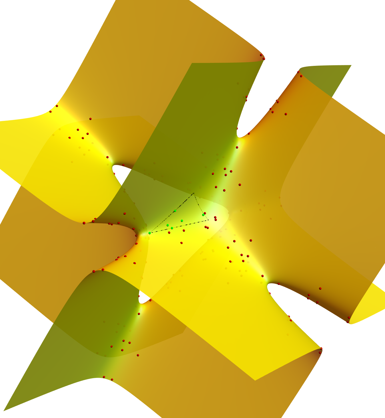
Figure 1. Lattice points and fundamental set (triangular) for $k=3685$.

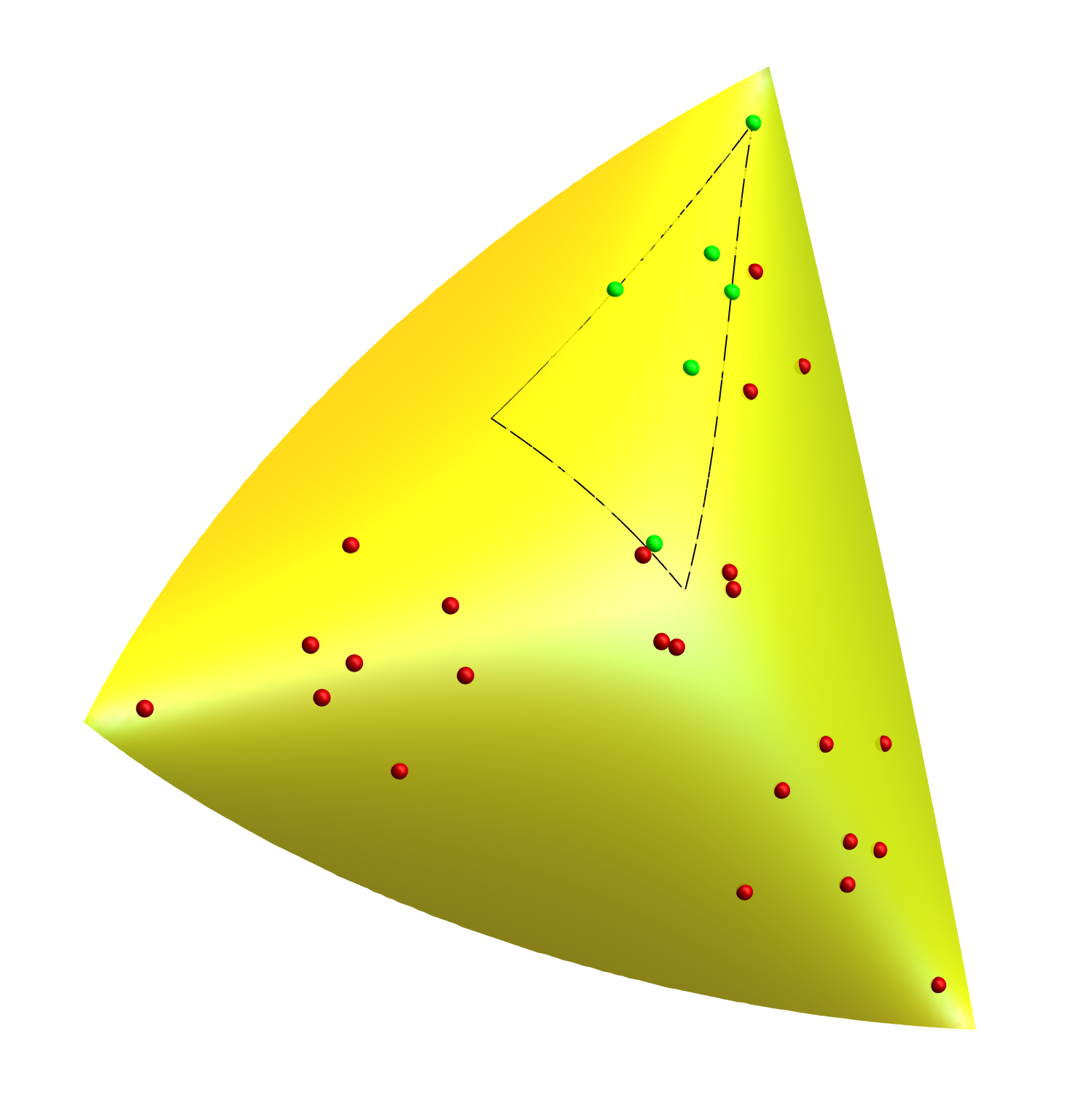
Figure 2. Closeup of fundamental set (triangular) for $k=3685$.

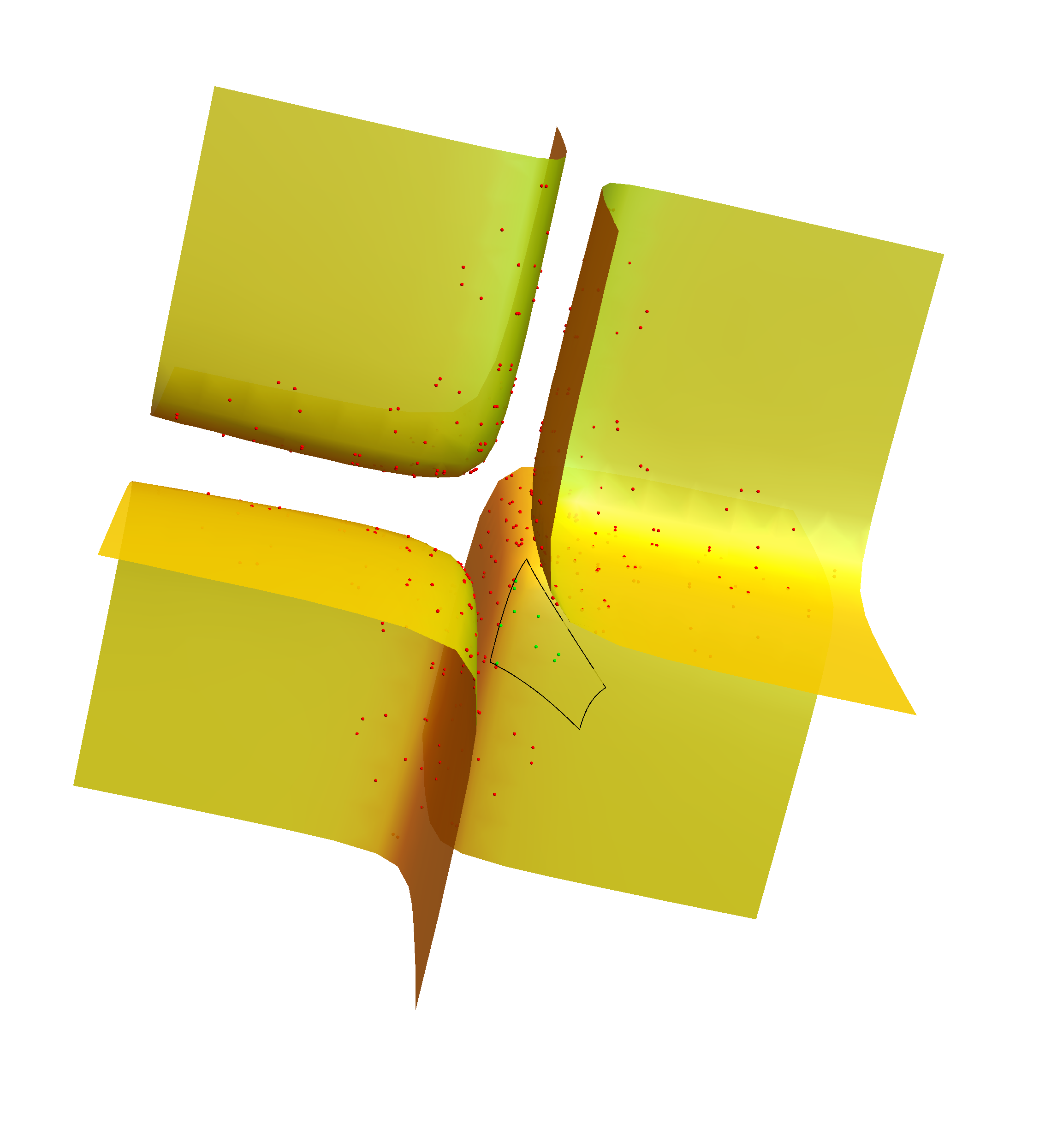
Figure 3. Lattice points and fundamental set for $k=-3691$.

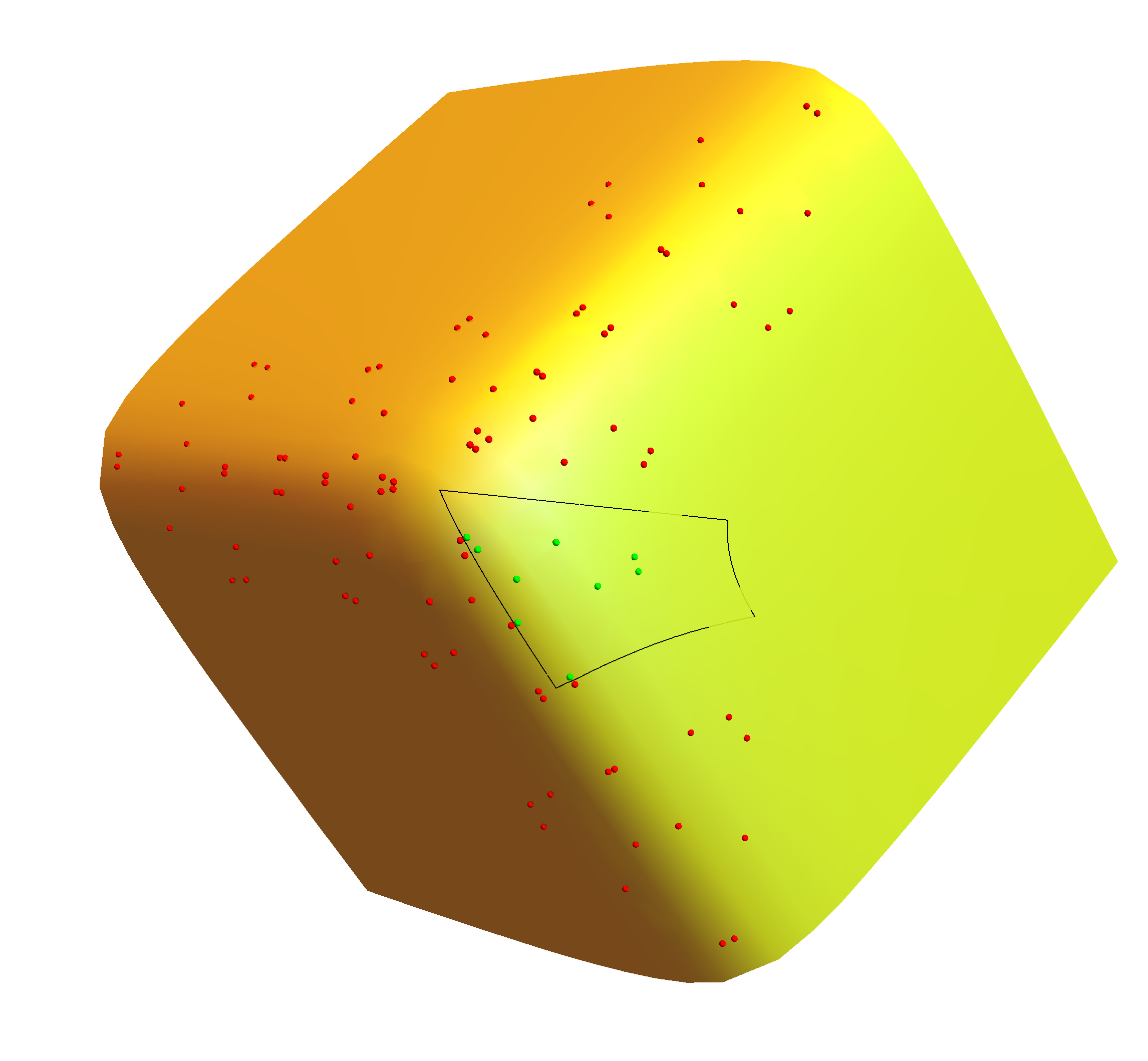
Figure 4. Closeup of fundamental set for $k=-3691$.

Some simple consequences of Theorem 1.1 are (see the discussion in Sec. 2 and also Secs. 7 and 8)  :

1. $V_{46}(\mathbb{Z})=\emptyset$, that is $\mathfrak{h}_{M}(46)=0$, this being the first positive Hasse failure  .

2. $\mathfrak{h}_{M}(-2)=1$ with all solutions equivalent to the point $(3,3,4)$; while $k=-4$ is the first negative Hasse failure  .

3. $\mathfrak{h}_{M}(k)\ll_{\varepsilon}|k|^{\frac{1}{3}+\varepsilon}$ as $k\to\pm\infty$. This follows from the fact that when considering the values taken by the corresponding indefinite quadratic form in the $y$ and $z$ variable, for each fixed $x$, the units are bounded in number due to the restrictions imposed by the fundamental sets  .

4. Let $\mathfrak{h}^{\pm}_{M}(k)=|\mathfrak{F}^{\pm}_{k}(\mathbb{Z})|$ where $\pm=\text{sgn}({k})$, this being defined for any $k$. Then Theorem 1.1 implies that for generic $k$, $\mathfrak{h}_{M}^{\pm}(k)=\mathfrak{h}_{M}(k)$ while otherwise $\mathfrak{h}_{M}(k)\leq\mathfrak{h}_{M}^{\pm}(k)$. We have

   (1.6) $$\sum_{\begin{subarray}{c}k\neq 4\\ |k|\leq K\end{subarray}}\mathfrak{h}_{M}^{\pm}(k)\sim C^{\pm}K(\log K)^{2},$$

   where $C^{\pm}>0$ and $K\to\infty$ (see Lemmas 7.2 and 7.3).

So, as expected in this case of critical dimension 3, the numbers $\mathfrak{h}_{M}(k)$ are small on average. On the other hand the fact that this average grows, albeit very slowly, is a key feature as it suggests that $\mathfrak{h}_{M}(k)$ might be non-zero for many $k$’s. In Section 10, we report on some numerical experiments using Theorem 1.1 to find the Hasse failures among the generic $k$’s when $0<k<6\times 10^{8}$. These suggest that

(1.7) $$\sum_{\begin{subarray}{c}0<k\leq K\\ k\,\text{admissible}\\ \mathfrak{h}_{M}(k)=0\end{subarray}}1\sim C_{0}K^{\theta},$$

with $C_{0}>0$ and $\theta\approx 0.8875..$ . We also provide results concerning other statistics for the $\mathfrak{h}_{M}(k)$’s for $k$ in this range (see Sec. 10 for the numerics concerning the numbers $\mathfrak{h}_{M}(k)$ and some conjectures that these support).

Our main result concerns the values assumed by $M$ and the Hasse failures in (1.7); we prove that $M$ is almost perfect but not perfect.

Theorem 1.2.

1. There are infinitely many Hasse failures. More precisely, the number of $0<k\leq K$ and $-K\leq k<0$ for which the Hasse Principle fails is at least $\sqrt{K}(\log K)^{-\frac{1}{2}}$ for $K$ large.

2. $M$ is almost perfect, that is

   $$\#\big{\{}|k|\leq K:\,k\ \text{admissible},\ \mathfrak{h}_{M}(k)=0\big{\}}=o(K)\,,$$

   as $K\to\infty$  and for almost all admissible $k$, $V_{k}(\mathbb{Z})$ is Zariski dense in $V_{k}$ .

Remark 1.3.

1. The proof of $(i)$ is based on quadratic reciprocity and a global factorization that arises for special $k$’s connected to the singular Cayley cubic $V_{4,M}$. If $k=4+\beta\nu^{2}$, with $\beta$ carefully chosen and $\nu$’s having its prime factors in certain arithmetic progressions, we show that $V_{k,M}(\mathbb{Z})=\emptyset$ even though $k$ is generic. Explicit examples are given in Sec. 8. Some of these obstructions to integer solutions are similar to ones found by Mordell [Mor53] for similar cubic equations, and also to the “Integer Brauer-Manin obstructions” in [CTW12]. Following our posting of an earlier version of this paper, [LM20] and [CTWX20] computed explicitly the Brauer groups of these affine Markoff surfaces, as well as the corresponding integral Brauer-Manin obstructions. They find that the Hasse failures in (i) and (ii) of Prop. 8.1 are accounted for by their obstructions. However, the analysis leading to Hasse failures in part (iii) of the Proposition uses both reciprocity and Markoff descent, and they are not accounted for by the integral Brauer-Manin obstruction alone. In any case, all of these algebraic obstructions are far fewer (they are of order of magnitude $\sqrt{K}$) than the Hasse failures that we found numerically, indicating that any simple description of the latter is perhaps not possible.

2. In the recent paper [GMS22], the Hasse failure (i) is exploited to give failures of profinite local to global principles for commutator equations in $SL_{2}(\mathcal{O})$ for $\mathcal{O}$ a ring of $S$-integers.

3. The proof of $(ii)$, when combined with Theorem 1.1 yields further information about the $\mathfrak{h}_{M}(k)$’s for generic $k$’s. If $t\geq 0$ is fixed, then

   $$\#\big{\{}0\leq|k|\leq K:\,\mathfrak{h}_{M}(k)=t,\ k\ \text{generic}\big{\}}=o(K),$$

   as $K\to\infty$ . So for generic $k$, $\mathfrak{h}_{M}(k)\to\infty$ for almost all $k$.

4. Our approach to proving that $M$ is full is to look for points in $V_{k,M}(\mathbb{Z})$ with $|k|\leq K$ in a region $\mathcal{R}$ where $x_{1}$ is small (roughly of size a power of $\log{K}$) and $x_{2},\ x_{3}$ vary in a sector (so they are of the same size). $\mathcal{R}$ is contained in the fundamental domains $\mathfrak{F}_{k}^{\pm}$ and retains the tentacles (cusps) of the latter, this being critical to ensuring that the average for $|k|\leq K$, of the number of points in $V_{k,M}(\mathbb{Z})\cap\mathcal{R}$ grows with $k$. For a given $x_{1}$, $M$ is a (indefinite) binary quadratic form in $x_{2},\ x_{3}$ and this allows one to use the methods developed in [BF11] and [BG06] to show that $M$ assumes a positive proportion of the $k$’s. Our proof that $M$ is full is much more delicate. As with the proofs that cubic forms in many variables (starting with the case of a sum of four cubes [Dav39]) represents almost all admissible numbers, we compare the number of points in $V_{k,M}(\mathbb{Z})\cap\mathcal{R}$, to an arithmetic function $\delta^{(m)}(k)$ (see Sec. 9; here $m$ is a secondary parameter) which is a product of local densities of solutions. While this heuristic for the count can be way off for certain $k$’s (e.g. for the Hasse failures), we show that its variance from the actual count when averaged over $k$, is small enough to conclude that for almost all $k$’s, $\delta^{(m)}(k)$ is a good approximation. The fullness then follows after showing that $\delta^{(m)}(k)$ is large for most $k$’s . That $M$ is almost perfect then follows from (1.5) and that $M$ is full. The proof of the vanishing of the variance boils down to examining the “diagonal” and “off-diagonal” terms in (9.15). For the first, we make use of the divisor analysis for varying quadratic forms [BG06], while for the second a modern treatment of Kloosterman’s method for ternary quadratic forms [Nie10] allows for uniform control of the contributions of the varying forms.

To end the introduction, we return to a discussion of the general affine cubic form $F$ in three variables. The study of the level sets $V_{k,M}(\mathbb{Z})$, for example (1.5) using the Markoff group is very special. It applies to $F$’s of the form $F=F_{0}+G$, where

(1.8) $$F_{0}=cx_{1}x_{2}x_{3}\quad{\rm and}\quad G=\sum_{i,j}a_{ij}x_{i}x_{j}+\sum_{i}a_{i}x_{i}+a,$$

with $a_{jj}=\pm 1$ for $j=1,\;2,\;3$ and $c,\;a,\;a_{ij},\;a_{i}\in\mathbb{Z}$, as well as $F$’s obtained from these via integral affine linear substitutions (see Appendix A). Among these special affine forms are ones for which $V_{k}$ carry explicit integral points and even parametric curves, for every $k$. This coupled with the action of the corresponding Markoff group leads to $V_{k}(\mathbb{Z})$ being Zariski dense for every $k$. Thus, the form is both perfect and ‘universal’ in the sense that it represents every $k$. Explicit examples are

(1.9) $$U_{1}(x_{1},x_{2},x_{3})=x_{1}+x_{1}^{2}+x_{2}^{2}+x_{3}^{2}-x_{1}x_{2}x_{3},$$

and

(1.10) $$U_{2}(x_{1},x_{2},x_{3})=x_{2}(x_{3}-x_{1})+x_{1}^{2}+x_{2}^{2}+x_{3}^{2}-x_{1}x_{2}x_{3}.$$

See Section 5 for an analysis of these forms. The only perfect $F$’s that we are aware of are of the form (1.8).

On the other hand, our treatment of the fullness of $M$ applies more generally. We leave the precise details and proofs of the following comments to a forthcoming paper. If $F_{0}$ is reducible in $\mathbb{Q}[x_{1},x_{2},x_{3}]$, then $F$ is full. In this case $F_{0}$ has a linear factor, which is the condition that $F$ has $\mathcal{h}$-invariant ([DL64]) equal to 1 (see Appendix A for a discussion of these arithmetic invariants of $F$). The linear factor yields a rational plane in $F_{0}(x_{1},x_{2},x_{3})=0$ which can be used as the small variable and to generate a family of planes and of binary quadratic forms and a tentacled region. If $F_{0}$ is irreducible in $\mathbb{Q}[x_{1},x_{2},x_{3}]$ then our moving plane method fails. Nevertheless one can still create tentacled regions $\mathcal{R}$ in $\mathbb{R}^{3}$ using neighborhoods at infinity of the curve $F_{0}({\bf x})=0$ in $\mathbb{P}^{2}(\mathbb{R})$. As before, on average over $k$ with $|k|\leq K$, the number of points $r_{\mathcal{R}}(k)$ in $V_{k,F}(\mathbb{Z})\cap\mathbb{R}$ grows slowly with $k$. The study of the variance of $r_{\mathcal{R}}(k)$ from its expected number (i.e. a product of local densities) reduces to counting points on the hypersurface $F({\bf x})-F({\bf y})=0$ with $({\bf x},{\bf y})\in\mathcal{R}\times\mathcal{R}$. While this is well beyond the available tools from the circle method, a natural hypothesis in this context along the lines of ([Hoo16]) would lead to $F$ being full. In particular, this applies to $F=S$ in (1.2). The much stronger suggestion that $S$ is perfect ([HB92]), which was mentioned at the start is a fascinating one, as is the question of the existence of any perfect homogeneous $F$. All $k$’s are admissible for the homogeneous form $x_{1}^{3}+x_{2}^{3}+2x_{3}^{3}$ and it is a candidate for being both perfect and universal. It is interesting to note that this form is universal when considered over the $S$-integer ring $\mathbb{Z}[\frac{1}{6}]$, and has infinitely many solutions for each $k$.

We point out that the analogous problem for quadratic polynomials in two variables is very different in that $f$ is never absolutely irreducible, and indeed the typical such $f$ is never full.

Finally, we note that the $V_{k,F}$’s for $F=M$ are the relative character varieties for the representations of $\pi_{1}(\Sigma_{1,1})$ into $SL_{2}$ (here $\Sigma_{g,n}$ is a surface of genus $g$ and $n$ punctures) and the group $\Gamma$ is essentially the mapping class group action on the $V_{k,M}$’s (see Goldman [Gol03]). As such, many of the questions that we address in this simplest case make sense with $\Sigma_{1,1}$ replaced by $\Sigma_{g,n}$ (see Whang [Wha20]). In particular it is shown there that the key feature that the integral points for these varieties consist of finitely many $\Gamma$-orbits, persists. However both for $\Sigma_{1,1}$ and in this more general setting, this finiteness fails when the integers are replaced by $S$-integers in a general number ring. This makes for a quite different picture and analysis to which we will return in a future work.

Acknowledgements.
We thank V. Blomer, E. Bombieri, J. Bourgain, T. Browning, C. McMullen, P. Whang and U. Zannier for insightful discussions.
AG thanks the Institute for Advanced Study and Princeton University for making possible visits during part of the years 2015-2017 when much of this work took place. He also acknowledges support from the IAS, the Simons Foundation and his home department. He dedicates this article to his family Priscilla, Armand and Saskia.
PS was supported by NSF grant DMS 1302952.
The softwares Eureqa${}^{\text{\textregistered}}$ and Mathematica^© were used on a PC running Linux to generate some of the data. Additional computations were done at the OSU-HPCC at Oklahoma State University, which is supported in part through the NSF grant OCI-1126330.

Notation 1.4.

For the remainder of the paper we suppress the reference to the Markoff equation. So for example $V_{k}$ would mean $V_{k,M}$. We also use $(\frac{*}{p})_{L}$ to denote the Legendre symbol $(\frac{*}{p})$ to avoid any confusion with fractions.

2. The descent argument revisited

The descent argument was first considered by Markoff in [Mar80], and later extended by Hurwitz [Hur07] and Mordell [Mor53] (see also [Bar94] for a study of fundamental solutions associated with a special case of these several variable hypersurfaces) . In particular, Hurwitz used a “height” function given by $h(x_{1},x_{2},x_{3})=|x_{1}|+|x_{2}|+|x_{3}|$, which was then utilized subsequently in the literature. The descent argument led to a finite number of points plus those with minimal height. Our initial analysis is a revisit of this descent argument but without the use of the height function (we later use a new function for a finer analysis).

For $k\in\mathbb{Z}$, consider the set of integral points on the Markoff surface

(2.1) $$V_{k}:\quad\quad x_{1}^{2}+x_{2}^{2}+x_{3}^{2}-x_{1}x_{2}x_{3}=k\,.$$

After invariance by permutations and also changing two signs but leaving out Vieta involutions (which we call narrow equivalence), we see that (i) if $k<0$, we may consider only solutions $0\leq x_{1}\leq x_{2}\leq x_{3}$, and (ii) if $k\geq 0$, there are two types of solutions namely those with all variables non-negative and so $0\leq x_{1}\leq x_{2}\leq x_{3}$; and those in the compact set $\mathfrak{S}^{+}(k)$ with exactly one negative variable and two positive.

For $k<0$ we note that $x=0$, $1$ or $2$ are not possible (since they give $k=x_{2}^{2}+x_{3}^{2}$, $4(k-1)=(2x_{2}-x_{3})^{2}+3x_{3}^{2}$ and $(x_{2}-x_{3})^{2}=k-4$ respectively) so that we assume $3\leq x_{1}\leq x_{2}\leq x_{3}$ in this case.

When $k\geq 0$, $x=0$ and $x=1$ give at most finitely many triples $(x_{1},x_{2},x_{3})$. and we denote this set by $\mathfrak{T}(k)$. Thus in this case, $(x_{1},x_{2},x_{3})$ is a solution implies it is equivalent (narrowly) to one in $\mathfrak{S}^{+}(k)\cup\mathfrak{T}(k)$ or it satisfies $2\leq x_{1}\leq x_{2}\leq x_{3}$.

We now consider the Vieta involution acting on $(x_{1},x_{2},x_{3})\rightarrow(x_{1},x_{2},x_{1}x_{2}-x_{3})$. If $x_{1}x_{2}-x_{3}<0$, so that $k\geq 0$, then $(x_{1},x_{2},x_{3})$ is equivalent to a solution in $\mathfrak{S}^{+}(k)$. Next suppose $x_{1}x_{2}-x_{3}\geq x_{3}$, so that $2x_{3}\leq x_{1}x_{2}$. Solving for $x_{3}$ in (2.1) gives $2x_{3}=x_{1}x_{2}\pm\sigma$ where $\sigma=\sqrt{x_{1}^{2}x_{2}^{2}-4(x_{1}^{2}+x_{2}^{2}-k)}$, so that necessarily $\sigma=x_{1}x_{2}-2x_{3}\leq(x_{1}-2)x_{2}$. Squaring and simplifying gives $(x_{1}-2)x_{2}^{2}\leq(x_{1}^{2}-k)$.

If $x_{1}\geq 3$ and $k>0$, we conclude that $x_{2}^{2}<x_{1}^{2}$, a contradiction. If $x_{1}=2$, we conclude that $k\leq 4$. Thus we derive a contradiction for all $k>4$, so that in this case we have $0\leq x_{1}x_{2}-x_{3}<x_{3}$. But more is true, namely $0\leq x_{1}x_{2}-x_{3}<x_{2}$ shown as follows: if $x_{2}\leq x_{1}x_{2}-x_{3}<x_{3}$, then $x_{1}x_{2}<2x_{3}\leq 2(x_{1}-1)x_{2}$, so that necessarily $2x_{3}=x_{1}x_{2}+\sigma$. Then $\sigma\leq(x_{1}-2)x_{2}$ and the argument above gives a contradiction. Hence we have

Lemma 2.1.

If $k>4$ and if $(x_{1},x_{2},x_{3})$ is a lattice point on $V_{k}$ in (2.1), it is equivalent to one in the compact set $\mathfrak{S}^{+}(k)\cup\mathfrak{T}(k)$ where

$$\mathfrak{S}^{+}(k)=\left\{(-x_{1},x_{2},x_{3}):\ 3\leq x_{1}\leq x_{2}\leq x_{3}\,;\ x_{1}^{2}+x_{2}^{2}+x_{3}^{2}+x_{1}x_{2}x_{3}=k\right\}\cap\mathbb{Z}^{3}\,,$$

or if not then it is equivalent to $(x_{1},x_{1}x_{2}-x_{3},x_{2})$, with $3\leq x_{1}x_{2}-x_{3}<x_{2}\leq x_{3}$ and $x_{1}\geq 3$.

The special cases $1\leq k\leq 3$ are settled as follows: (i) there are no solutions when $k=3$ since there are none modulo 4; (ii) for $k=2$, we can use the descent argument above and conclude that we need only look for solutions to $x^{2}+y^{2}+z^{2}+xyz=2$ with all variables non-negative or we solve the Markoff equation with $x_{1}\in\{0,\pm 1,\pm 2\}$, giving us the point $(0,1,1)$ and its infinite orbit under $\Gamma$; and for $k=1$, the same analysis results in the point $(0,0,1)$, for which there is only a finite orbit under $\Gamma$. The cases $k=0$ and $4$ we consider in the next sections (they correspond to the original Markoff surface in Sec. 3.1 and the singular Cayley surface in Sec. 4.3).

For $k<0$, the estimate $(x_{1}-2)x_{2}^{2}\leq(x_{1}^{2}-k)$ given above is still valid when we assume $x_{1}x_{2}-x_{3}\geq x_{3}$, with $3\leq x_{1}\leq x_{2}\leq x_{3}$. Then, if $x_{1}\geq 4$, it follows that $2x_{2}^{2}\leq x_{1}^{2}+|k|$, which then implies $x_{2}\leq\sqrt{|k|}$, so that $x_{3}\leq\frac{x_{1}x_{2}}{2}\leq\frac{|k|}{2}$. If $x_{1}=3$, then clearly $x_{2}\leq\sqrt{9+|k|}$, and so $x_{3}\leq\frac{3}{2}\sqrt{9+|k|}$. The same argument shows that for large values of $|k|$, $x_{1}\ll|k|^{\frac{1}{3}}$, $x_{2}\ll\sqrt{\frac{|k|}{x_{1}}}$ and $x_{3}\ll\sqrt{|k|x_{1}}$. Next, supposing $x_{2}\leq x_{1}x_{2}-x_{3}<x_{3}$, we see that the point $(x_{1},x_{2},x_{3})$ is $\Gamma$-equivalent to $(y_{1},y_{2},y_{3})=(x_{1},x_{2},x_{1}x_{2}-x_{3})$, where now $y_{1}y_{2}-y_{3}\geq y_{3}$, the same inequality considered above. Thus we have

Lemma 2.2.

For $k<0$, if $(x_{1},x_{2},x_{3})$ is a lattice point on $V_{k}$ in (2.1), it is then equivalent to one in the compact set $\mathfrak{S}^{-}(k)\subset\mathfrak{U}(k)$, where

$$\mathfrak{S}^{-}(k):=\left\{(x_{1},x_{2},x_{3}):3\leq x_{1}\leq x_{2}\leq x_{3}\leq\frac{1}{2}x_{1}x_{2}\right\}\cap V_{k}(\mathbb{Z})\,,$$

and

$$\mathfrak{U}(k):=\left\{(x_{1},x_{2},x_{3}):3\leq x_{1}\leq x_{2}\leq\sqrt{|k|+9};\ 3\leq x_{3}\leq\frac{3}{2}(|k|+9)\right\}\,,$$

or if not it is equivalent to $(x_{1},x_{1}x_{2}-x_{3},x_{2})$ with $3\leq x_{1}x_{2}-x_{3}<x_{2}\leq x_{3}$ and $x_{1}\geq 3$.

The lemmas above form the basis of the descent argument with repeated application of the Vieta involution so that ultimately any integral solution is equivalent to one in a corresponding finite set.

3. Bhargava cubes and Markoff

To construct the fundamental sets in the next section, we utilize a function $\Delta({\bf x})$ given in (3.1), that proves useful in tracking the images of points under the action of the group $\Gamma$. While we could define $\Delta$ without comment, we give here our original construction using Bhargava cubes.

Let $x_{1}$, $x_{2}$ and $x_{3}$ be arbitrary integers and consider the Bhargava cube ([Bha04]) as shown in Fig. 5.

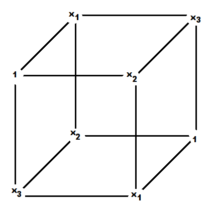
Figure 5. Bhargava cube associated with $M$.

The Bhargava slicings give rise to the three matrix pairs:

$$M_{1}=\left(\begin{array}[]{cc}1&x_{2}\\ x_{3}&x_{1}\end{array}\right)\ ,\quad N_{1}=\left(\begin{array}[]{cc}x_{1}&x_{3}\\ x_{2}&1\end{array}\right)\ ;$$

$$M_{2}=\left(\begin{array}[]{cc}1&x_{3}\\ x_{1}&x_{2}\end{array}\right)\ ,\quad N_{2}=\left(\begin{array}[]{cc}x_{2}&x_{1}\\ x_{3}&1\end{array}\right)\ ;$$

$$M_{3}=\left(\begin{array}[]{cc}1&x_{1}\\ x_{2}&x_{3}\end{array}\right)\ ,\quad N_{3}=\left(\begin{array}[]{cc}x_{3}&x_{1}\\ x_{2}&1\end{array}\right).$$

These in turn give the following three quadratic forms $Q_{i}(u,v)$, where

$$Q_{1} =(x_{2}x_{3}-x_{1})u^{2}+(1+x_{1}^{2}-x_{2}^{2}-x_{3}^{2})uv+(x_{2}x_{3}-x_{1})v^{2}\,,$$

$$Q_{2} =(x_{1}x_{3}-x_{2})u^{2}+(1+x_{2}^{2}-x_{1}^{2}-x_{3}^{2})uv+(x_{1}x_{3}-x_{2})v^{2}\,,$$

$$Q_{3} =(x_{1}x_{2}-x_{3})u^{2}+(1+x_{3}^{2}-x_{1}^{2}-x_{2}^{2})uv+(x_{1}x_{2}-x_{3})v^{2}\,.$$

All three quadratic forms have the same discriminant $\Delta=\Delta(x_{1},x_{2},x_{3})$ which also factorizes to give

(3.1) $$\begin{split}\Delta&=(1+x_{2}^{2}-x_{1}^{2}-x_{3}^{2})^{2}-4(x_{1}x_{3}-x_{2})^{2}\,,\\ &=(1+x_{1}+x_{2}+x_{3})(1+x_{2}-x_{1}-x_{3})(1+x_{3}-x_{1}-x_{2})(1+x_{1}-x_{2}-x_{3})\,.\end{split}$$

Note that

1. $\Delta\equiv 0$ or $1\,({\rm mod}\,4)$ depending on if $x_{1}^{2}+x_{2}^{2}+x_{3}^{2}$ is odd or even respectively.

2. $\Delta$ is invariant under permutations.

3. $\Delta$ is invariant if one variable is fixed and the sign is changed on the other two variables.

4. If $2\leq x_{1}\leq x_{2}\leq x_{3}$, then $\Delta<0$ if and only if $x_{2}\leq x_{3}\leq x_{1}+x_{2}-2$.

3.1. The case $k=0$

Recall (Markoff [Mar80]) that the solution set has two orbits with fundamental roots $(0,0,0)$ and $(3,3,3)$. We have $\Delta(0,0,0)=1$ and $\Delta(3,3,3)=-80$. We show here that

(3.2) $$\Delta(x_{1},x_{2},x_{3})<0\ \ \text{if and only if}\ \ (x_{1},x_{2},x_{3})=(3,3,3).$$

Thus, the two orbits each have a minimal value for $\Delta$, taken at the associated fundamental roots. In other words, there are two components of $V_{0}(\mathbb{Z})$ and in each component $\Delta$ has a minimum value, taken at a unique point, which can then be used as a generator for that component. This phenomenon repeats itself when $k\geq 5$ below.

We prove (3.2) as follows: since $x_{1}^{2}+x_{2}^{2}+x_{3}^{2}=x_{1}x_{2}x_{3}$, it follows that $x_{1}$, $x_{2}$ and $x_{3}$ are all positive or exactly two are negative (we avoid the trivial solution here). By the properties of $\Delta$ itemized above, we may assume that $1\leq x_{1}\leq x_{2}\leq x_{3}$. The Markoff equation is equivalent to the equation $(x_{1}^{2}-4)(x_{2}^{2}-4)-16=(2x_{3}-x_{1}x_{2})^{2}$, from which it follows that $3\leq x_{1}\leq x_{2}\leq x_{3}$, which we assume. Suppose $\Delta(x_{1},x_{2},x_{3})<0$, so that $x_{2}\leq x_{3}\leq x_{1}+x_{2}-2<2x_{2}$. Solving for $x_{3}$ in the Markoff equation gives us $2x_{3}=x_{1}x_{2}\pm\sigma$, where $\sigma=\sqrt{(x_{1}x_{2})^{2}-4(x_{1}^{2}+x_{2}^{2})}\geq 1$.

If $x_{1}\geq 4$ we must discard the positive sign since $x_{3}<2x_{2}$. So in this case, $x_{1}x_{2}-\sigma=2x_{3}\geq 2x_{2}$, from which, by expanding and simplifying, one gets $4x_{2}^{2}\leq x_{1}x_{2}^{2}\leq x_{1}^{2}+2x_{2}^{2}\leq 3x_{2}^{2}$, a contradiction.

For $x_{1}=3$, we have $x_{2}\leq x_{3}\leq x_{1}+x_{2}-2=x_{2}+1$, so that $x_{3}=x_{2}$ or $x_{3}=x_{2}+1$. If $x_{3}=x_{2}$, we have $9+2x_{2}^{2}-3x_{2}^{2}=0$ so that $x_{1}=x_{2}=x_{3}=3$. Finally if $x_{3}=x_{2}+1$, we must have $9+x_{2}^{2}+(x_{2}+1)^{2}=3(x_{2}^{2}+x_{2})$, which is impossible.

4. Fundamental sets and Theorem 1.1

The descent arguments of Markoff, Hurwitz and Mordell show that there is a finite set of lattice points from which all lattice points of the Markoff surface (2.1) can be obtained as images under $\Gamma$. This section provides a proof of Theorem 1.1 by showing the inequivalence of the points in the finite set.

4.1. The case $k\geq 5$

Recall from Sec. 2 that if $k\geq 5$, any solution ${\bf x}=(x_{1},x_{2},x_{3})$ to the Markoff equation (2.1) is equivalent to one in a compact reduced set (by Lemma 2.1 and descent). We order the coordinates first such that $0\leq|x_{1}|\leq|x_{2}|\leq|x_{3}|$.

In the next section, we show that the Markoff equation has no solutions for those $k$’s (positive or negative) satisfying any of the following congruences: $k\equiv 3\,({\rm mod}\,4)$ and $k\equiv\pm 3\,({\rm mod}\,9)$, these then accounting for $\frac{5}{12}K+O(1)$ members in the interval $5\leq k\leq K$, and we call them non-admissible; the non-admissible $k$’s have local obstructions. The remaining $k$’s we call admissible, and there are $\mathcalorig{A}(K)=\frac{7}{12}K+O(1)$ of them.

We say that $k$ is exceptional if there is a solution to (2.1) with $|x_{j}|=0,1$ or $2$; these $k$’s satisfy at least one of the equations (i) $u^{2}+v^{2}=k$ , (ii) $u^{2}+3v^{2}=4(k-1)$, or (iii) $u^{2}=k-4$. Consequently, for $k$’s in an interval of length $K$, they account for at most $O\left(K(\log{K})^{-\frac{1}{2}}\right)$ members, and we will ignore them in what follows. The remaining $\frac{7}{12}K+O\left(K(\log{K})^{-\frac{1}{2}}\right)$ numbers $k$ in the interval $5\leq k\leq K$ we shall call generic.

It follows from Sec. 2 that every solution ${\bf x}$ associated to a generic $k$ is equivalent to one in the set $\mathfrak{S}^{+}(k)$ given in Lemma 2.1. We now show that the elements in this set, when non-empty, are inequivalent under $\Gamma$, so that $\mathfrak{S}^{+}(k)$ is a fundamental set.

We will use the $\Delta$-function given in (3.1) to form an ordering on the tree of solutions to the Markoff equation. Given any ${\bf x}=(x_{1},x_{2},x_{3})$, the three Vieta maps are $\mathcal{V}_{1}:(x_{1},x_{2},x_{3})\mapsto(x_{2}x_{3}-x_{1},x_{2},x_{3})$, $\mathcal{V}_{2}:(x_{1},x_{2},x_{3})\mapsto(x_{1},x_{1}x_{3}-x_{1},x_{3})$ and $\mathcal{V}_{3}:(x_{1},x_{2},x_{3})\mapsto(x_{1},x_{2},x_{1}x_{2}-x_{3})$. Recall that the group $\Gamma$ is generated by permutations, double sign-changes and the Vieta maps. The $\Delta$-function is invariant under the first two motions and we denote $\Delta_{i}=\Delta\circ\mathcal{V}_{i}$. Then, it is easy to check that when ${\bf x}$ is a solution of the Markoff equation, one has

(4.1) $$\Delta_{1}({\bf x})-\Delta({\bf x})=x_{2}x_{3}(x_{2}x_{3}-2x_{1})\left[2(k-5)+(x_{2}^{2}-4)(x_{3}^{2}-4)\right],$$

$$\Delta_{2}({\bf x})-\Delta({\bf x})=x_{1}x_{3}(x_{1}x_{3}-2x_{2})\left[2(k-5)+(x_{1}^{2}-4)(x_{3}^{2}-4)\right],$$

$$\Delta_{3}({\bf x})-\Delta({\bf x})=x_{1}x_{2}(x_{1}x_{2}-2x_{3})\left[2(k-5)+(x_{1}^{2}-4)(x_{2}^{2}-4)\right].$$

The expressions in the square brackets in all three formulae above are strictly positive when $k$ is generic and if ${\bf x}$ is any solution of the corresponding Markoff equation.

We set up the tree associated with solutions as follows: each solution ${\bf x}=(x_{1},x_{2},x_{3})$ will be a vertex and neighboring vertices are edge connected if they are obtained from ${\bf x}$ by one of the three Vieta maps. As such, we identify coordinates if they are obtained by permutations or double sign changes (noting that $\Delta$ is unchanged under them). By this latter identification, the coordinates are one of two types, namely all positive or exactly one negative. It is then possible to rearrange them into the following canonical forms: $(x_{1},x_{2},x_{3})$ or $(-x_{1},x_{2},x_{3})$ with $3\leq x_{1}\leq x_{2}\leq x_{3}$. We call the former positive nodes and the latter negative nodes. By Lemma 2.1, for $k\geq 5$, every positive node is equivalent to a negative node (or otherwise, by descent is equivalent to the node $(3,3,3)$ which corresponds to $k=0$).

We look at the action of the Vieta maps on a positive node. It is clear that $x_{2}x_{3}-2x_{1}$ and $x_{1}x_{3}-2x_{2}$ are strictly positive so that $\Delta_{1}({\bf x})>\Delta({\bf x})$ and $\Delta_{2}({\bf x})>\Delta({\bf x})$. Moreover, the nodes $\mathcal{V}_{1}({\bf x})$ and $\mathcal{V}_{2}({\bf x})$ are both positive, Next, the argument showing descent in Sec. 2 shows that $x_{1}x_{2}-2x_{3}\geq 0$ is impossible so that $\Delta_{3}({\bf x})<\Delta({\bf x})$. Here $\mathcal{V}_{3}({\bf x})$ may be either positive or negative. We represent these observations by the images Fig.6a and Fig.6b , where square nodes are positive nodes, disc nodes are negative nodes, dark nodes are the Vieta images while the original point is a light node (the vertical ordering of the nodes is determined by the signs of the $\Delta$-differences from (4.1)).

Next, if we begin with a negative node (so that one replaces $x_{1}$ with $-x_{1}$ in the formulae above, it is obvious that $\Delta_{i}({\bf x})>\Delta({\bf x})$ for all $i$ and (after a double sign change and reordering) that the $\mathcal{V}_{i}({\bf x})$ are all positive. This is represented by Fig. 6c .

It follows now that the tree decomposes into components and each component has a root that is a negative node. Moreover, the negative node occupies the lowest point on the tree, with all other nodes in that component being positive (in other words, $\Delta$ has a minimum on each component and that minimum is determined by a negative node). Thus the negative nodes form a fundamental set, giving us the first case of Theorem 1.1.

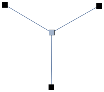
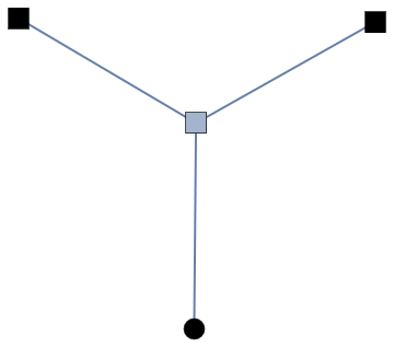
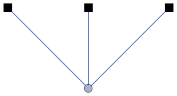
Figure 6. Node blocks; top: (a), (b); bottom: (c).

4.2. The case $k<0$

From Sec. 2 and Lemma 2.2 every lattice point in $V_{k}$ is equivalent to one in $\mathfrak{S}^{-}(k)$. We show that the points in this set are inequivalent. First using $(x_{1}^{2}-4)(x_{2}^{2}-4)=(2x_{3}-x_{1}x_{2})^{2}-4(k-4)$ in (4.1) and the similar formulae with the variables permuted, we see that the three terms in square brackets in (4.1) are all positive. Thus the signs of the differences of the $\Delta$-functions in (4.1) are determined by the three terms $x_{2}x_{3}-2x_{1}$, $x_{1}x_{3}-2x_{2}$ and $x_{1}x_{2}-2x_{3}$. The first two are obviously positive, and one sees that the last is non-negative if and only if $(x_{1},x_{2},x_{3})\in\mathfrak{S}^{-}(k)$ Thus, in the tree determined by these points one sees that we have nodes of the type shown in Fig.6(c) with two or three black square vertices emanating from points in $\mathfrak{S}^{-}(k)$, while for points in the complementary set, we have nodes of the type in Fig.6(a). It follows that the points in $\mathfrak{S}^{-}(k)$ can serve as the roots of the components of the tree, from which the second case of Theorem 1.1 follows.

4.3. The Cayley surface $k=4$

Most of the argument above for $k\geq 5$ can be applied to the case $k=4$, and we indicate the necessary modifications. First, we consider solutions of the type $(-x_{1},x_{2},x_{3})$ with $x_{1},\,x_{2},\,x_{3}\geq 0$ satisfying $x_{1}^{2}+x_{2}^{2}+x_{3}^{2}+x_{1}x_{2}x_{3}=4$. It is obvious that there are only two solutions up to equivalence, namely $(-2,0,0)\sim(0,0,2)$ and $(-1,1,1)\sim(1,1,2)$. Hence we need only consider solutions of the type $(x_{1},x_{2},x_{3})$ with $0\leq x_{1}\leq\ x_{2}\leq x_{3}$. If $x_{1}=0$, the only solution is $(0,0,2)$ while if $x_{1}=1$, then the only choice is $(1,1,2)$. Then by the descent argument in Sec. 2, if $x_{1}\geq 3$, the solution $(x_{1},x_{2},x_{3})$ is equivalent to one with one of the coordinates equal to 2. It is trivial that the only solutions of this kind are one of the type $(2,a,a)$, with $a\geq 0$ integers. It suffices now to check the equivalence of these solutions. It is easily checked that the orbits of $(2,0,0)$, $(2,1,1)$ and $(2,2,2)$ contain no other points of the type $(2,a,a)$ except themselves, so that we assume $a\geq 3$.

Following the three formulas in (4.1), if ${\bf x}=(2,a,a)$, then two of the Vieta transformations keep it inert while the third creates a node above it, this new node not being of the same type (we say “above” to mean $\Delta_{i}({\bf x})>\Delta({\bf x})$). Also following the argument used for $k\geq 5$, if ${\bf x}=(x_{1},x_{2},x_{3})$, with $x_{i}\geq 3$, then two Vieta transformations create nodes above it while a third creates a node below it. It is then easily seen that a tree containing a node of the type $(2,a,a)$ cannot contain a different node of the same type. Hence we have

Proposition 4.1.

The Cayley surface $V_{4}(\mathbb{Z})$ has infinitely many inequivalent orbits, each determined by a solution of the type $(2,a,a)$, with $a\geq 0$.

One checks that the $(2,0,0)\sim(-2,0,0)$-component has only 1 element (upto permutation and double sign-change) and so the minimal $\Delta$-value is $\Delta(-2,0,0)=9$. Next, the $(2,1,1)$-component has only 2 elements namely $(2,1,1)$ and $(-1,1,1)$. The minimal $\Delta$-value is $\Delta(-1,1,1)=-16$ while $\Delta(2,1,1)=5$. Finally, $\Delta(2,a,a)=9-4a^{2}<0$ for $a\geq 2$. Then the same argument used in Sec. 3.1 can be used to show that any lattice point $\bf{x}$ not of these type satisfy $\Delta({\bf x})\geq 0$, so that the minimal $\Delta$-value is uniquely determined. Thus, even here each component has a unique minimal $\Delta$-value, whose point can be used as a generator.

Remark 4.2.

One can use the $\Delta$-function and the analysis above to deduce a descent procedure. One concludes that either every positive node descends to a negative node or if not, there is an infinite chain of positive nodes on which $\Delta({\bf x})$ is strictly decreasing. The latter is not possible since $\Delta({\bf x})\geq 0$ on positive nodes. There are only finitely many negative nodes in $\mathfrak{S}^{+}(k)$. So we conclude that there are finitely many orbits. Repeating the analysis in the paper also shows that all the negative points are $\Gamma$-inequivalent and in each orbit $\Delta$ has a minimum value taken at the root of that orbit, so at the only (modulo double sign-changes) negative point on that orbit.

Using Lagrange multipliers on the region on $V_{k}$ with $x_{j}\geq 3$ and $k\to\infty$, one can show that :

1. $$\min_{{\bf x}\in\mathfrak{S}^{+}(k)}\Delta({\bf x})\ \geq\ k^{2}+18k^{\frac{3}{2}}+88k+\frac{621}{4}k^{\frac{1}{2}}+O(1);$$

2. $$\max_{{\bf x}\in\mathfrak{S}^{-}(k)}\Delta({\bf x})\ \leq\ k^{2}-18k^{\frac{3}{2}}+88k-\frac{45}{4}k^{\frac{1}{2}}+O(1);$$

3. $$\min_{{\bf x}\in\mathfrak{S}^{-}(k)}\Delta({\bf x})\ \geq\ -3k^{\frac{4}{3}}+O(k).$$

Hence asymptotically, $\Delta$ behaves like a Minkowski gauge-function, with "successive minima" taken at the root of the orbits; that is if $\mathfrak{h}(k)$ is the number of orbits, the first $\mathfrak{h}(k)$ minimal values (counted with multiplicity) of $\Delta$ on the lattice points on $V_{k}$ occur at the negative points.

5. Parametric solutions on Markoff-type surfaces and Zariski density.

We show in this section that for generic $k$, the Markoff surface has no parametric integral points and that the solution set is Zariski dense. We also consider the surfaces given by $U_{1}$ and $U_{2}$ mentioned in the Introduction.

5.1. Parametric solutions

Lemma 5.1.

For any $k\in\mathbb{Z}$, let $M^{*}_{k}$ be the surface given by $M^{*}({\bf x})=k$, where

(5.1) $$M^{*}({\bf x})=\sum_{j=1}^{3}\alpha_{j}x_{j}+\left(\beta_{1}x_{2}x_{3}+\beta_{2}x_{1}x_{3}+\beta_{3}x_{1}x_{2}\right)+x_{1}^{2}+x_{2}^{2}+\varepsilon x_{3}^{2}-x_{1}x_{2}x_{3},$$

where $\varepsilon=\pm 1$ and $\alpha_{j}$, $\beta_{j}\in\mathbb{Z}$ for all $j$. Suppose there are polynomials $P_{j}(t)\in\mathbb{Z}[t]$ each with non-zero degree, such that $M^{*}(P_{1},P_{2},P_{3})=k$ identically in $t$. Then there are polynomials $Q_{1},Q_{2}\in\mathbb{Z}[t]$ of non-zero degree and a constant $q\in\mathbb{Z}$ such that $M^{*}(q,Q_{1},Q_{2})=k$ identically in $t$.

Proof.

Let $P_{j}$ have degree $d_{j}\neq 0$ for $j=1,2,3$ as above. By comparing degrees in (5.1) we cannot have $d_{1}=d_{2}=d_{3}$, so that there is either a unique $d_{j}$ exceeding the other two or exactly two of the degrees are the same. The latter does not happen as it implies that at least one of the polynomials is a constant. Hence (comparing degrees in (5.1)) we have that $d^{\prime\prime}=d^{\prime}+d$ for some choice of the degrees. It will not matter which subscript represents the largest degree in what follows, so that we put $d_{3}=d_{1}+d_{2}$, with $d_{1}$, $d_{2}\geq 1$.

There is a Vieta affine transformation acting on the surface given by $x_{3}\mapsto x_{4}=x_{1}x_{2}-\alpha_{3}-\beta_{1}x_{2}-\beta_{2}x_{1}-\varepsilon x_{3}$, so that if $P_{4}(t)$ is the polynomial determined by $x_{4}$, we have

$$P_{3}P_{4}=k-P_{1}^{2}-P_{2}^{2}-\beta_{3}P_{1}P_{2}-\alpha_{1}P_{1}-\alpha_{2}P_{2},$$

identically in $t$. If $d_{4}$ is the degree of $P_{4}$, we have $d_{3}+d_{4}\leq 2\max(d_{1},d_{2})$, so that $d_{4}\leq\max(d_{1},d_{2})-\min(d_{1},d_{2})<\max(d_{1},d_{2})$. Thus we have polynomials $P_{1},P_{2},P_{4}$ in place of $P_{1},P_{2},P_{3}$ representing integral points on the surface, with the maximal degree reduced by at least one and the new maximum degree is determined by $P_{1}$ or $P_{2}$. Either $P_{4}$ has degree zero, in which case we are done, or if not, all the new polynomials have non-zero degree. Repeating this descent argument (with a different Vieta transformation) shows that there must be parametric solutions with at least one polynomial constant, and the other two polynomials of non-zero degree. ∎

It is not possible to have parametric solutions to (5.1) with two of the polynomials constant. It follows from the lemma that if parametric solutions exist then there exists $q\in\mathbb{Z}$ and $Q_{1},Q_{2}\in\mathbb{Z}[t]$ of the same degree $d$ satisfying (5.1) (it is possible to show that $d\leq 2$, if it exists). We now consider some special cases:

1. For the Markoff equation we have $Q_{1}^{2}+Q_{2}^{2}-qQ_{1}Q_{2}=k-q^{2}$. Comparing the highest degree term shows that there are integers $q_{1},q_{2}$ such that $q_{1}^{2}+q_{2}^{2}-qq_{1}q_{2}=0$. It follows that $q=\pm 2$ and $k-4=\square$. Moreover if $k=4+w^{2}$, then one has a parametric family of solutions $q=2$, $Q_{1}=t$ and $Q_{2}=t+w$. In particular, this means that if $k$ is generic, there are no parametric solutions to the associated Markoff level set.

2. Consider the Markoff-like surface $x_{1}^{2}+x_{2}^{2}-x_{3}^{2}-x_{1}x_{2}x_{3}=k$. If we have parametric solutions as above of the type $(Q_{1},Q_{2},q)$, then the argument is identical to the Markoff case so that we conclude there are no such parametric solutions except when $k+4=w^{2}$, in which case we have the parametric family $(t+w,t,2)$. Next, if either $x_{1}$ or $x_{2}$ is $q$, we have the equation $Q_{1}^{2}-Q_{2}^{2}-qQ_{1}Q_{2}=k-q^{2}$, so like the case above, we have $q_{1}^{2}-q_{2}^{2}-qq_{1}q_{2}=0$. We conclude that $q=0$ so that when $k\neq 0$, $Q_{1}$ and $Q_{2}$ have degree zero, a contradiction. When $k=0$, we have the parametric family $(Q_{1},0,\pm Q_{1})$ for any polynomial $Q_{1}$.

   Remark 5.2.

   This surface has the following features: (i) there are no local obstructions, (ii) for $k=4^{\alpha}k^{\prime}$ with $\alpha\geq 0$ and $k^{\prime}$ odd, it has the integral points $(0,2^{\alpha}\frac{k^{\prime}+1}{2},2^{\alpha}\frac{k^{\prime}-1}{2})$, (iii) if $k^{\prime}\neq 1$ or $\alpha\geq 3$, there are infinitely many integral points, and (iv) there are infinitely many Hasse failures (in particular, $k=94$ is a Hasse failure). This latter statement follows from an analysis similar to that in Prop. 8.1.

3. Consider the linear deformation $U_{1}$ of the Markoff equation considered in (1.9), namely $x_{1}+x_{1}^{2}+x_{2}^{2}+\varepsilon x_{3}^{2}-x_{1}x_{2}x_{3}=k$. For any integer $k$, and $\varepsilon=\pm 1$, we have the parametric family of integral solutions $\left(-t^{2}+k-4\varepsilon,-t^{2}+t+k-4\varepsilon,2\right)$ .

4. Consider the quadratic deformation $U_{2}$ of (1.10): $x_{2}x_{3}-x_{1}x_{2}+x_{1}^{2}+x_{2}^{2}+x_{3}^{2}-x_{1}x_{2}x_{3}=k$. For any $k$, we have the parametric solutions $(-t^{2}+t+k-1,-t^{2}+k-1,1)$.

5.2. Zariski density

5.2.1.

We prove (1.5) for the Markoff surface for $k$ not a square (this ensures that if $V_{k,M}(\mathbb{Z})\neq\emptyset$, then it has a lattice point with at most one coordinate zero). First note that if $\hat{{\bf x}}=(\hat{x}_{1},\hat{x}_{2},\hat{x}_{3})\in V_{k}(\mathbb{Z})$ and $|\hat{x}_{j}|\geq 2$ for some $j$, then $|V_{k}(\mathbb{Z})|=\infty$. To see this, say $|\hat{x}_{1}|\geq 2$; then the composition of the Vieta transformation $\mathcal{V}_{3}$ with the permutation of $x_{2}$ and $x_{3}$ yields the transformation $(x_{1},x_{2},x_{3})\mapsto(x_{1},x_{1}x_{2}-x_{3},x_{2})$ in $\Gamma$. This preserves the plane $x_{1}=\hat{x}_{1}$ and $V_{k}$, and it induces the linear action $\left[\begin{array}[]{cc}\hat{x}_{1}&-1\\ 1&\ 0\end{array}\right]$ on this plane. Since $|\hat{x}_{1}|\geq 2$, this element in $SL_{2}(\mathbb{Z})$ is of infinite order, so that its orbit is infinite (since it is not acting on the origin) and its Zariski closure contains the conic section $\{x_{1}=\hat{x}_{1}\}\cap V_{k}$. We now argue as in [CZ06]. If $\overline{V_{k}(\mathbb{Z})}$, the Zariski closure of $V_{k}(\mathbb{Z})$ is not $V_{k}$, then it is contained in a finite union of curves in $V_{k}$. Hence there can be at most finitely many $\hat{x}_{1}$’s with $(\hat{x}_{1},\hat{x}_{2},\hat{x}_{3})\in V_{k}(\mathbb{Z})$ with $|\hat{x}_{1}|\geq 2$ (since otherwise $\overline{V_{k}(\mathbb{Z})}$ contains infinitely many distinct conic sections as above). The same applies to $\hat{x}_{2}$ and $\hat{x}_{3}$, giving $|V_{k}(\mathbb{Z})|<\infty$. That is we have shown that $|V_{k}(\mathbb{Z})|=\infty$ implies that $\overline{V_{k}(\mathbb{Z})}=V_{k}$. To complete the proof of (1.5) note that if $|k|>20$ and $(\hat{x}_{1},\hat{x}_{2},\hat{x}_{3})\in V_{k}(\mathbb{Z})$ then for at least one of the $j$’s, $|\hat{x}_{j}|\geq 2$ and so $|V_{k}(\mathbb{Z})|\neq\emptyset$ implies $\overline{V_{k}(\mathbb{Z})}=V_{k}$. For the $k$’s with $|k|\leq 20$ we check directly that (1.5) holds. One can show that when $k=1,\ 9,\ 49$, for example, $V_{k,M}(\mathbb{Z})\neq\emptyset$ but has only a finite orbit. On the other hand, when $k=k_{1}^{2}$ with $k_{1}$ having an odd prime factor congruent to one modulo 4, then $V_{k,M}(\mathbb{Z})$ has an infinite orbit, and by the argument above, is Zariski dense.

5.2.2.

We next consider the surface $U_{1}$ discussed above and in (1.9). The argument is almost the same as for the Markoff surface except that now we have an affine transformation and a lack of full symmetry in the variables.

As in the case for the Markoff equation, assume that $\overline{V_{k,U_{1}}(\mathbb{Z})}\neq V_{k,U_{1}}$ so that it is contained in a finite union of curves. Consider the two Vieta transformations: $\mathcal{V}_{1}({\bf x})=(x_{2}x_{3}-1-x_{1},x_{2},x_{3})$ and $\mathcal{V}_{3}({\bf x})=(x_{1},x_{2},x_{1}x_{2}-x_{3})$, keeping $x_{2}$ fixed. Put ${\bf w}=(x_{1},x_{3})^{T}$ so that $\mathcal{V}_{1}$ and $\mathcal{V}_{3}$ act on ${\bf w}$. By abuse of notation, we have

$$\mathcal{V}_{1}({\bf w})=\left[\begin{array}[]{cc}-1&x_{2}\\ 0&\ 1\end{array}\right]{\bf w}+\left[\begin{array}[]{c}-1\\ 0\end{array}\right]\quad\text{and}\quad\mathcal{V}_{3}({\bf w})=\left[\begin{array}[]{cc}1&0\\ -x_{2}&-1\end{array}\right]{\bf w},$$

so that we write $\mathcal{V}_{1}\mathcal{V}_{3}({\bf w})=A{\bf w}+{\bf b}$, with

$$A=\left[\begin{array}[]{cc}-1-x_{2}^{2}&-x_{2}\\ -x_{2}&\ -1\end{array}\right]\in SL(2,\mathbb{Z}),\quad\text{and}\quad{\bf b}=\left[\begin{array}[]{c}-1\\ 0\end{array}\right].$$

Hence $(\mathcal{V}_{1}\mathcal{V}_{3})^{n}{\bf w}=A^{n}{\bf w}+\sum_{j=0}^{n-1}A^{j}{\bf b}$ for $n\geq 1$. If $\mathcal{V}_{1}\mathcal{V}_{3}$ has order $n$, it follows that $(A^{n}-I)[(A-I){\bf w}+{\bf b}]=0$. Now, if $x_{2}\neq 0$, then $A$ has infinite order and $A^{n}-I$ is invertible, so that we have $(A-I){\bf w}=-{\bf b}$. This is impossible since $(A-I)^{-1}{\bf b}$ is not integral. Hence $\mathcal{V}_{1}\mathcal{V}_{3}$ has infinite order so that the orbit $\mathcal{V}_{1}\mathcal{V}_{3}(x_{1},x_{2},x_{3})$ with $x_{2}\neq 0$ fixed is infinite. The assumption of Zariski density implies that there are only finitely many $x_{2}$’s.

Since the surface given by $U_{1}$ is symmetric in $x_{2}$ and $x_{3}$, it follows that there are only finitely many $x_{2}$ and $x_{3}$’s, from which we conclude that there are at most finitely many lattice points (since $x_{1}$ is determined). Starting with the base point ${\bf p}=(k-4,k-4,2)$ which is on the surface, we see that this is impossible since the orbit $\mathcal{V}_{1}\mathcal{V}_{3}({\bf p})$ is infinite if $k\neq 4$. Hence $V_{k,U_{1}}(\mathbb{Z})$ is Zariski dense in $V_{k,U_{1}}$ for all $k\neq 4$. For $k=4$, we use instead ${\bf p}=(-1,2,0)$ so that ${\bf w}\neq{\bf 0}$, and the argument above gives an infinite orbit, and Zariski dense.

5.2.3.

The argument for $U_{2}$ is almost identical: we use the Vieta transformations $\mathcal{V}_{1}({\bf x})=(x_{2}x_{3}+x_{2}-x_{1},x_{2},x_{3})$ and $\mathcal{V}_{3}({\bf x})=(x_{1},x_{2},x_{1}x_{2}-x_{2}-x_{3})$, and have the corresponding matrix equation for $\mathcal{V}_{1}\mathcal{V}_{3}({\bf w})=A{\bf w}+{\bf b}$, with

$$A=\left[\begin{array}[]{cc}-1+x_{2}^{2}&-x_{2}\\ x_{2}&\ -1\end{array}\right]\in SL(2,\mathbb{Z}),\quad\text{and}\quad{\bf b}=\left[\begin{array}[]{c}-x_{2}^{2}+x_{2}\\ -x_{2}\end{array}\right].$$

The analysis is the same as for $U_{1}$ except now we have that $A^{n}-I$ is invertible if $|x_{2}|\geq 3$. As above, we derive a contadiction of the finite order assumption since $(A-I)^{-1}{\bf b}$ is not integral. In particular, taking the base point ${\bf p}=(k-1,k-1,1)$, we conclude that $V_{k,U_{2}}(\mathbb{Z})$ is infinite if $|k|\geq 4$. The reasoning above using the Zariski density assumption shows that there are only finitely many $x_{2}$’s.

Due to the lack of symmetry in the variables, we redo the analysis with $x_{1}$ fixed, using $\mathcal{V}_{2}\mathcal{V}_{3}({\bf w})=A{\bf w}+{\bf b}$, with $\mathcal{V}_{2}({\bf x})=(x_{1},x_{1}x_{3}+x_{1}-x_{3}-x_{2},x_{3})$, $\mathcal{V}_{3}$ as before, ${\bf w}=(x_{2},x_{3})^{T}$ and

$$A=\left[\begin{array}[]{cc}(x_{1}-1)^{2}-1&1-x_{1}\\ x_{1}-1&\ -1\end{array}\right]\in SL(2,\mathbb{Z}),\quad\text{and}\quad{\bf b}=\left[\begin{array}[]{c}x_{1}\\ 0\end{array}\right].$$

If $|x_{1}-1|\geq 3$, we conclude $(A-I){\bf w}=-{\bf b}$, and derive a contradiction regarding the finite order assumption. Thus the Zariski density hypothesis implies that there are only finitely many $x_{1}$’s. Hence, again since $x_{3}$ is determined by $x_{1}$ and $x_{2}$, $V_{k,U_{2}}(\mathbb{Z})$ is finite, giving a contradiction. Thus $V_{k,U_{2}}(\mathbb{Z})$ is Zariski dense in $V_{k,U_{2}}$ for all $|k|\geq 4$. For $|k|\leq 4$, a direct computation gives many eligible candidates for lattice points that lead to Zariski dense.

A much stronger theorem concerning $\Gamma$ invariant holomorphic curves and structures for the surfaces corresponding to (1.8) is proved in ([CL09], Theorem D).

6. Local solutions in $\mathbb{Z}_{p}$

Proposition 6.1.

Given $k\in\mathbb{Z}$, the congruence $x_{1}^{2}+x_{2}^{2}+x_{3}^{2}-x_{1}x_{2}x_{3}\equiv k\,({\rm mod}\,p^{n})$ has solutions for all primes $p$ and $n\geq 1$ except for the following exceptions : $k\equiv 3\,({\rm mod}\,4)$, $k\equiv\pm 3\,({\rm mod}\,9)$.

We break up the proof into several cases.

It is particularly easy to verify the Proposition for powers of primes $p\geq 5$ as follows: recall the Fricke trace identity, namely for any real unimodular matrices $A$ and $B$,

(6.1) $$\mathfrak{S}(A)^{2}+\mathfrak{S}(B)^{2}+\mathfrak{S}(AB)^{2}-\mathfrak{S}(A)\mathfrak{S}(B)\mathfrak{S}(AB)=\mathfrak{S}([A,B])+2,$$

where $[A,B]=ABA^{-1}B^{-1}$ is the commutator, and $\mathfrak{S}()$ denotes the trace of the matrix.

Restricting the matrices to $SL(2,\mathbb{Z})$, one obtains integral solutions to (2.1), with $k=t+2$, where we denote $\mathfrak{S}([A,B])$ by $t$. We have

Lemma 6.2.

For any prime $p\geq 5$, $n\geq 1$ and any integer $t$, there exists matrices $A,\,B\,\in SL(2,\mathbb{Z}/p^{n}\mathbb{Z})$ such that

$$\mathfrak{S}(A)^{2}+\mathfrak{S}(B)^{2}+\mathfrak{S}(AB)^{2}-\mathfrak{S}(A)\mathfrak{S}(B)\mathfrak{S}(AB)\equiv t+2\,({\rm mod}\,p^{n})\,.$$

Proof.

For

$$A=\begin{bmatrix}a&b\\ c&d\end{bmatrix},\quad B=\begin{bmatrix}e&0\\ 0&f\end{bmatrix},\quad A,B\in SL(2,\mathbb{Z}/p^{n}\mathbb{Z}),$$

we have $\mathfrak{S}([A,B])=2adef-bc(e^{2}+f^{2})\equiv 2-bc(e-f)^{2}\,({\rm mod}\,p^{n})$.

Since $p\geq 5$, there exists $e$ and $f$ such that $(e-f,p)=1$ with $ef\equiv 1\,({\rm mod}\,p^{n})$. Then, we choose $c$ so that $c(e-f)^{2}\equiv 1\,({\rm mod}\,p^{n})$. Finally, we choose $a=1$, $b=2-t$ and $d=1+bc$.∎∎

Corollary 6.3.

For $p\geq 5$ and $n\geq 1$, the Markoff congruence $x_{1}^{2}+x_{2}^{2}+x_{3}^{2}-x_{1}x_{2}x_{3}\equiv k\,({\rm mod}\,p^{n})$ has the solution $x_{1}\equiv 2-(k-4)c$, $x_{2}\equiv e+f$ and $x_{3}\equiv e-f+fx_{1}$, with $e,\,f$ and $c$ as in the proof of the Lemma.

The argument above gives the existence of solutions for powers of $p\geq 5$. It is useful to have a precise count for the number of solutions modulo $p$. For this, it is not any harder to consider the more general problem in

Lemma 6.4.

For $p\geq 3$, let $N_{p}$ denote the number of solutions to $x_{1}^{2}+x_{2}^{2}+x_{3}^{2}-\alpha x_{1}x_{2}x_{3}\equiv\beta$ modulo $p$. Then

$$N_{p}=\left\{\begin{array}[]{ll}p^{2}+p\left(\frac{-\beta}{p}\right)_{\!\!L}&\text{if}\ p|\alpha,\\ \\ p^{2}+1+\left(\frac{\alpha^{2}\beta-4}{p}\right)_{\!\!L}\left[3+\left(\frac{\beta}{p}\right)_{\!\!L}\right]p&\quad\text{otherwise}.\end{array}\right.$$

Proof.

It is clear we need only consider the cases $\alpha=0$ and $\alpha=1$, the latter when $p\nmid\alpha$, upon which we multiply through with $\alpha^{2}$ and change variables.

Write $S_{p}(a)=\sum_{u}e_{p}(au^{2})$ (where $e_{p}(x)=e^{\frac{2\pi ix}{p}}$) so that when $p\nmid a$, one has $S_{p}(a)=\left(\frac{a}{p}\right)_{\!\!L}S_{p}(1)$. When $\alpha=1$, putting $u\equiv 2x_{3}-x_{1}x_{2}\,({\rm mod}\,p)$ shows that we have the same number of solutions as the congruence

$$4(x_{1}^{2}+x_{2}^{2})+u^{2}-x_{1}^{2}x_{2}^{2}\equiv 4\beta\,({\rm mod}\,p),$$

so that

(6.2) $$N_{p}-p^{2}=\frac{1}{p}\sum_{a\not\equiv 0}T_{p}(a)S_{p}(a)e_{p}(-4a\beta)\,;$$

here we obtained $p^{2}$ solutions when $a\equiv 0\,({\rm mod}\,p)$, and we put

$$T_{p}(a)=\sum_{x_{1},x_{2}}e_{p}\left(a(4x_{1}^{2}+4x_{2}^{2}-x_{1}^{2}x_{2}^{2})\right)=\sum_{x_{1}}e_{p}(4ax_{1}^{2})S_{p}\left(a(4-x_{1}^{2})\right)\,.$$

Breaking the sum over $x_{1}$ in $T_{p}$ above depending on when $x_{1}\equiv\pm 2$ or not gives us

$$T_{p}(a)=2p\,e_{p}(16a)+\left(\frac{a}{p}\right)_{\!\!L}S_{p}(1)\sum_{x_{1}}\left(\frac{4-x_{1}^{2}}{p}\right)_{\!\!L}e_{p}(4ax_{1}^{2}).$$

Summing over $a$ in (6.2) gives $N_{p}=p^{2}+\mathcalorig{E}_{1}+\mathcalorig{E}_{2}$, where

(6.3) $$\mathcalorig{E}_{1}=2S_{p}(1)\sum_{a}\left(\frac{a}{p}\right)_{\!\!L}\,e_{p}\left(a(16-4\beta)\right)=2S_{p}(1)^{2}\left(\frac{4-\beta}{p}\right)_{\!\!L}\,,$$

and

(6.4) $$\mathcalorig{E}_{2}=\frac{1}{p}S_{p}(1)^{2}\sum_{x_{1}}\left(\frac{4-x_{1}^{2}}{p}\right)_{\!\!L}\ \sum_{a\not\equiv 0}e_{p}\left(4a(x_{1}^{2}-\beta)\right).$$

Summing over $a$ in (6.4), we write $\mathcalorig{E}_{2}=-\mathcalorig{E}_{2,1}+\mathcalorig{E}_{2,2}$ with

$$\mathcalorig{E}_{2,1} =\frac{S_{p}(1)^{2}}{p}\sum_{x_{1}^{2}\not{\equiv}\beta}\ \left(\frac{4-x_{1}^{2}}{p}\right)_{\!\!L}\ ,$$

$$=\frac{S_{p}(1)^{2}}{p}\left[\sum_{x_{1}}\ \left(\frac{4-x_{1}^{2}}{p}\right)_{\!\!L}-\left(\frac{4-\beta}{p}\right)_{\!\!L}\left[1+\left(\frac{\beta}{p}\right)_{\!\!L}\right]\right],$$

and

$$\mathcalorig{E}_{2,2}=\frac{S_{p}(1)^{2}}{p}(p-1)\left(\frac{4-\beta}{p}\right)_{\!\!L}\left[1+\left(\frac{\beta}{p}\right)_{\!\!L}\right].$$

Since $\sum_{x}\left(\frac{4-x_{1}^{2}}{p}\right)_{\!\!L}=-\left(\frac{-1}{p}\right)_{\!\!L}$, it follows from (6.3) and (6.4) that

$$N_{p}=p^{2}+2S_{p}(1)^{2}\left(\frac{4-\beta}{p}\right)_{\!\!L}+\frac{S_{p}(1)^{2}}{p}\left(\frac{-1}{p}\right)_{\!\!L}+S_{p}(1)^{2}\left(\frac{4-\beta}{p}\right)_{\!\!L}\left[1+\left(\frac{\beta}{p}\right)_{\!\!L}\right].$$

Using $S_{p}(1)^{2}=p\left(\frac{-1}{p}\right)_{\!\!L}$ then gives us

$$N_{p}=p^{2}+\left(\frac{\beta-4}{p}\right)_{\!\!L}\left[3+\left(\frac{\beta}{p}\right)_{\!\!L}\right]p+1.$$

It follows that $N_{p}\geq p^{2}-4p+1=(p-2)^{2}-3>0$ if $p\geq 5$. This is also true of $p=3$ as can be checked with different values of $\beta$.

Next, if $p|\alpha$,

$$N_{p}-p^{2}=\frac{1}{p}\sum_{a\not\equiv 0}e_{p}(-\beta a)S_{p}(a)^{3}=\frac{S_{p}(1)^{3}}{p}\sum_{a}e_{p}(-\beta a)\left(\frac{a}{p}\right)_{\!\!L}.$$

If $p|\beta$, then $N_{p}=p^{2}$. If $p\nmid\beta$, then the right hand side is $p\left(\frac{-\beta}{p}\right)_{\!\!L}$.

6.1. Prime powers : $p\geq 5$

We have already considered this case in Corollary 6.3, but for completeness we give here the argument using Hensel’s lemma. Let $f=x_{1}^{2}+x_{2}^{2}+x_{3}^{2}-x_{1}x_{2}x_{3}-k$, considered as three functions of each variable. Then $f^{\prime}$ takes the following three forms: $2x_{1}-x_{2}x_{3}$, $2x_{2}-x_{1}x_{3}$ or $2x_{3}-x_{1}x_{2}$. To obtain solutions modulo $p^{n+1}$ from those modulo $p^{n}$, it suffices that at least one of these derivatives not vanish modulo $p^{n}$. We call such triples non-singular. If $(x_{1},x_{2},x_{3})$ is such a non-singular solution modulo $p^{n}$ with say $2x_{1}-x_{2}x_{3}\not\equiv 0\,({\rm mod}\,p^{n})$, then Hensel’s lemma gives a solution to $f\equiv 0\,({\rm mod}\,p^{n+1})$ of the form $(y_{1},x_{2},x_{3})$ with $y_{1}\equiv x_{1}\,({\rm mod}\,p^{n})$. This new triple is non-singular modulo $p^{n+1}$ so that by induction a non-singular solution modulo $p$ lifts to one modulo $p^{n}$ for any $n\geq 1$, for any prime $p\geq 5$. Note that $(3,3,3)$ is a non-singular solution when $p|k$, giving solutions modulo $p^{n}$.

Next suppose the triple $(x_{1},x_{2},x_{3})$ is a singular solution of the congruence $f\equiv 0\,({\rm mod}\,p)$ for $p\nmid k$, so that we have $2x_{1}\equiv x_{2}x_{3}$, $2x_{2}\equiv x_{1}x_{3}$ and $2x_{3}\equiv x_{1}x_{2}\,({\rm mod}\,p)$. If we assume $p\nmid x_{1}x_{2}x_{3}$, then necessarily $x_{1}^{2}\equiv x_{2}^{2}\equiv x_{3}^{2}$ and $x_{1}x_{2}x_{3}\equiv 2x_{1}^{2}\,({\rm mod}\,p)$. Substituting into $f\equiv 0\,({\rm mod}\,p)$ gives $x_{1}^{2}\equiv k\,({\rm mod}\,p)$ so that $k$ must be a non-zero quadratic residue modulo $p$, so say $k\equiv u^{2}\,({\rm mod}\,p)$. But then $(u,0,0)$ is a non-singular solution to $f\equiv 0\,({\rm mod}\,p)$, and so by above, lifts to a non-singular solution modulo $p^{n}$ for all $n\geq 1$.

Finally, suppose $p|x_{1}x_{2}x_{3}$ with $(x_{1},x_{2},x_{3})$ singular. Then $p$ divides $x_{1}$, $x_{2}$ and $x_{3}$, so that $p^{2}|k$. But then $(3,3,3)$ is a non-singular solution modulo $p^{2}$ for all $p>3$. We can now apply Hensel’s lemma as above, starting modulo $p^{2}$ and lifting to solutions modulo $p^{n}$ for all $n\geq 2$ and $p>3$.

6.2. Prime powers : $p=3$

The congruence $f\equiv 0\,({\rm mod}\,3)$ has the following non-singular solutions : when $k\equiv 1$, take $(1,0,0)$; and when $k\equiv-1$, take $(0,1,1)$. These solutions lift to solutions modulo $3^{n}$ for $n\geq 1$.

When $k\equiv 0\,({\rm mod}\,3)$, the only solution is the singular $(0,0,0)$. We now consider this case modulo 9. Since $3$ divides each of $x_{1}$, $x_{2}$ and $x_{3}$, then necessarily when $k\equiv 3$ or $6$ mod $9$, there are no solutions. So assume $9|k$, in which case $(3,0,0)$ is a non-singular solution modulo 9 and so lifts to solutions modulo $3^{n}$, $n\geq 2$.

6.3. Prime powers : $p=2$

Modulo 2, $f^{\prime}\equiv$ $x_{1}x_{2}$ or $x_{1}x_{3}$ or $x_{2}x_{3}$. Thus if $k$ is even, one may use the non-singular solution $(1,1,1)$ to obtain solutions modulo powers of 2. When $k$ is odd, the only solution is the singular $(0,0,1)$. Then necessarily $k\equiv 3\,({\rm mod}\,4)$ has no solutions. So assume $k\equiv 1\,({\rm mod}\,4)$ and we find the non-singular solution $(1,0,0)$ modulo 4 (note that here one uses $f^{\prime}\equiv 2x_{1}-x_{2}x_{3}\not\equiv 0\,({\rm mod}\,4)$). This then lifts to higher powers of 2.

7. The average of $\mathfrak{h}_{M}^{\pm}(k)$: counting lattice points.

We show here that the average of $\mathfrak{h}_{M}^{\pm}(k)$ is $C^{\pm}(\log{k})^{2}$, by counting lattice points in the domains given in Theorem 1.1 ((see the paragraph containing (1.6) for definitions). We provide the details for $k>5$.

Fix $u_{1}=a$ with $3\leq a\ll K^{\frac{1}{3}}$ and write $u_{2}=m$ and $u_{3}=n$. We determine the asymptotics of $N_{a}(K)$, the number of pairs $(m,n)$ satisfying the inequality $a^{2}+m^{2}+n^{2}+amn\leq K$ with $a\leq m\leq n$. We have

$$m\leq n\leq\frac{1}{2}\left(-am+\sqrt{4(K-a^{2})+(a^{2}-4)m^{2}}\right)\,,$$

so that $m\leq K_{a}$, with $K_{a}=\sqrt{\frac{K-a^{2}}{a+2}}$. Hence

$$N_{a}(K)=\frac{1}{2}\sum_{a\leq m\leq K_{a}}\left\{\sqrt{4(K-a^{2})+(a^{2}-4)m^{2}}-(a+2)m\right\}+O\left(\sqrt{\frac{K}{a}}\right)\,.$$

The function in the sum is decreasing in $m$ and the contribution from the endpoints are $O(\sqrt{K})$. Hence

$$N_{a}(K)=\frac{1}{2}\int_{a}^{K_{a}}\left\{\sqrt{4(K-a^{2})+(a^{2}-4)x^{2}}-(a+2)x\right\}dx+O\left(\sqrt{K}\right)\,.$$

Changing variables gives

$$N_{a}(K)=2\frac{K-a^{2}}{\sqrt{a^{2}-4}}\int_{\alpha}^{\beta}\left\{\sqrt{1+x^{2}}-\frac{a+2}{\sqrt{a^{2}-4}}x\right\}dx+O\left(\sqrt{K}\right)\,,$$

where $\beta=\frac{\sqrt{a-2}}{2}$ and $\alpha=O(aK^{-\frac{1}{2}})$. Replacing $\alpha$ with zero gives an error of $O(\sqrt{K})$ and the integral becomes

$$\frac{1}{2}\left\{\beta\sqrt{1+\beta^{2}}+\log{\left(\beta+\sqrt{1+\beta^{2}}\right)}-\frac{a+2}{\sqrt{a^{2}-4}}\beta^{2}\right\}\,.$$

Simplifying gives us

Lemma 7.1.

For $3\leq a\ll K^{\frac{1}{3}}$, the number of pairs $(m,n)$ satisfying the inequality $a^{2}+m^{2}+n^{2}+amn\leq K$ with $a\leq m\leq n$ is

$$N_{a}(K)=\log{\left[\frac{\sqrt{a-2}+\sqrt{a+2}}{2}\right]}\frac{K-a^{2}}{\sqrt{a^{2}-4}}+O(\sqrt{K}).$$

Lemma 7.2.

Let $R^{+}(K)$ be the number of points $(x_{1},x_{2},x_{3})$ satisfying $x_{1}^{2}+x_{2}^{2}+x_{3}^{2}+x_{1}x_{2}x_{3}\leq K$, with $3\leq x_{1}\leq x_{2}\leq x_{3}$  . Then

$$R^{+}(K)=\frac{1}{36}K(\log{K})^{2}+O(K\log{K})\,.$$

Proof.

It follows from the previous lemma that

$${}R^{+}(K)=\sum_{{3\leq a\leq K^{\frac{1}{3}}}}\,\log{\left[\frac{\sqrt{a-2}+\sqrt{a+2}}{2}\right]}\frac{K}{\sqrt{a^{2}-4}}+O\left(K^{\frac{5}{6}}\right).$$

The main term is asymptotic to $\frac{K}{2}\sum_{a}\frac{\log{a}}{a}\sim\frac{K}{4}(\log{K^{\frac{1}{3}}})^{2}$  .∎

We also state, without details, the analogous count for the case of $k<0$ in Theorem 1.1(ii).

Lemma 7.3.

Let $R^{-}(K)$ be the number of points $(x_{1},x_{2},x_{3})$ satisfying $x_{1}^{2}+x_{2}^{2}+x_{3}^{2}-x_{1}x_{2}x_{3}=-k$, with $0<k\leq K$ and $3\leq x_{1}\leq x_{2}\leq x_{3}\leq\frac{1}{2}x_{1}x_{2}$ . Then

$$R^{-}(K)=\frac{1}{48}K(\log{K})^{2}+O(K\log{K})\,.$$

8. Failures of the Hasse Principle

The fundamental sets allows us to determine Hasse failures for small $k$ very readily. For example, direct computations reveal that the smallest positive Hasse failure occurs with $k=46$. That $k=46$ is a Hasse failure can be verified by applying Theorem 1.1 as follows: either $k=46$ is exceptional or there exist $3\leq x_{1}\leq x_{2}\leq x_{3}$ such that $x_{1}^{2}+x_{2}^{2}+x_{3}^{2}+x_{1}x_{2}x_{3}=46$. The latter cannot occur since the smallest value of the polynomial is $54$. To determine if $46$ is exceptional, since it is not a sum of two squares and since 42 is not a square, it remains to check if the equation $x_{2}^{2}+x_{3}^{2}-x_{2}x_{3}=45$ has any solutions with $x_{2},\ x_{3}\ \in\mathbb{Z}$. The equation implies that $3|x_{2}$ and $3|x_{3}$, so that we consider the solvability of $y_{1}^{2}+y_{2}^{2}-y_{1}y_{2}=5$. This is equivalent to the solvability of $u_{1}^{2}+3u_{2}^{2}=20$, which is impossible by congruence modulo 5 or otherwise.

Let $V_{k}(\mathbb{Z})$ denote the integral points on the surface $x_{1}^{2}+x_{2}^{2}+x_{3}^{2}-x_{1}x_{2}x_{3}=k$, for $k\in\mathbb{Z}$. For $k=4+d$, the surface $V_{k}$ is the singular Cayley surface when reduced modulo $d$. Its features, coupled with global quadratic reciprocity, yield failures of strong approximation (mod $4d$). For example, assume that $n\to\left(\frac{4d}{n}\right)$ is a primitive Dirichlet character (mod $4d$) and let $S_{d}\subset\mathbb{Z}/4d\mathbb{Z}$ be the multiplicative closed set $\left\{n\ :\ \left(\frac{4d}{n}\right)=0\ \text{or}\ 1\right\}$. Then, for any ${\bf x}=(x_{1},x_{2},x_{3})\in V_{k}(\mathbb{Z})$ one has

(8.1) $$x_{j}^{2}-4\in S_{d}\ (\text{mod}\ 4d)\ ,\ \text{for}\ j=1,2,3\ .$$

These congruences on $x_{j}$ imposed by (8.1) are not consequences of local considerations and so strong approximation fails for $V_{k}(\mathbb{Z})$, at least (mod $4d$).

To see (8.1), we rewrite (2.1) as

(8.2) $$w^{2}-4d=\left(x_{1}^{2}-4\right)\left(x_{2}^{2}-4\right)\ ,$$

with $w=2x_{3}-x_{1}x_{2}$. Now, if $x_{1}^{2}-4=p_{1}p_{2}\ldots p_{l}$ with $p_{j}$ primes (possibly with repetition), then $w^{2}\equiv 4d\ (\text{mod}\ p_{j})$ and hence $\left(\frac{4d}{p_{j}}\right)=0$ or $1$. Thus $p_{j}\in S_{d}$ for each $j$, and hence so does $x_{1}^{2}-4$. The same applies to $x_{2}^{2}-4$ and $x_{3}^{2}-4$. Quadratic reciprocity then implies that the $x_{j}$’s must lie in certain congruence classes (mod $4d$).

As we now show, by specializing the $k$’s and enhancing the analysis above, we can eliminate all the candidate congruence classes and produce families of Hasse failures. We turn to these and the proof of Theorem 1.2(i) in the Introduction, which follows from Prop. 8.1 below.

Proposition 8.1.

For the following choices of $k$, $V_{k}(\mathbb{Z})$ is empty but $V_{k}(\mathbb{Z}_{p})$ is non-empty for all primes $p$ :

1. For $k<0$, choose $k=4-2\nu^{2}$, with odd $\nu$ having all its prime factors congruent to $1$ or $3$ modulo 8.

2. For $k>4$, choose $k=4+2\nu^{2}$ with $\nu$ having all of its prime factors in the congruence classes $\{\pm 1\}$ modulo 8, and in addition with $\nu\in\{0,\ \pm 3,\ \pm 4\}$ modulo 9.

3. Suppose $\ \ell\geq 13$ is a prime number with $\ell\equiv\pm 4$ (mod 9). Then choose $k=4+2\ell^{2}$.

The smallest positive $k$ here is 342.

Proof.

Writing $k=4+2\epsilon\nu^{2}$ with $\epsilon=\pm 1$, with odd $\nu$, the congruence conditions ensure that Prop. 6.1 implies $V_{k}(\mathbb{Z}_{p})\neq\varnothing$ for all primes $p$.

Let $(x_{1},x_{2},x_{3})$ be a solution to

(8.3) $$x_{1}^{2}+x_{2}^{2}+x_{3}^{2}-x_{1}x_{2}x_{3}=4+2\epsilon\nu^{2}\ ,$$

with the corresponding

(8.4) $$w^{2}-8\epsilon\nu^{2}=(x_{1}^{2}-4)(x_{2}^{2}-4)\ ,$$

with $w=2x_{3}-x_{1}x_{2}$.

Since $\nu$ is odd, $4\pm 2\nu^{2}$ is not divisible by 4, so that at least one of $x_{1}$, $x_{2}$ or $x_{3}$ is odd, so say $x_{1}$. Then $x_{1}^{2}-4\equiv 5\equiv-3\ (\text{mod}\ 8)$.

Case (i): It follows that $x_{1}^{2}-4$ is divisible by a prime number $q\equiv-1\ \text{or}\ -3\ (\text{mod}\ 8)$. Since $q\nmid\nu$, it follows from (8.4) that $-2$ is a quadratic residue modulo $q$, a contradiction.

Case (ii): It follows that $x_{1}^{2}-4$ is divisible by a prime number $q\equiv\pm 5\ (\text{mod}\ 8)$. Since $q\nmid\nu$, it follows from (8.4) that $2$ is a quadratic residue modulo $q$, a contradiction.

Case (iii): Recall that for $k\geq 5$, if $k$ is not exceptional, every solution is equivalent to one in the fundamental set $3\leq x_{1}\leq x_{2}\leq x_{3}$ with $x_{1}^{2}+x_{2}^{2}+x_{3}^{2}+x_{1}x_{2}x_{3}=k=4+2\ell^{2}$. This implies that $3\leq x_{1}\leq k^{\frac{1}{3}}$ and $x_{1}\leq x_{2}\leq\left(\frac{k}{x_{1}}\right)^{\frac{1}{2}}$. Now, the proof above requires that at least one of the variables is odd; but in fact at least 2 variables are odd (by considering the equation modulo 4). It follows that we derive a contradiction if we follow the proof above with $q\neq\ell$. On the other hand, if $q=\ell$, since two variables are odd, we can choose one, say $x_{1}$ satisfying $3\leq x_{1}\leq\sqrt{\frac{k}{3}}$ with $\ell|(x_{1}^{2}-4)$. Then $\ell|(x_{1}-2)$ or $\ell|(x_{1}+2)$ so that $x_{1}+2\geq\ell t$ for some $t\geq 1$. Then we get

$$\ell-2\leq\ell t-2\leq x_{1}\leq\sqrt{\frac{4+2\ell^{2}}{3}}\ ,$$

so that $3(\ell-2)^{2}\leq 4+2\ell^{2}$, which implies that $\ell<13$, a contradiction.

To complete the proof, it remains to check that our choice of $k$ is not exceptional, that is there are no solutions with say $x_{1}$ equal to $0$, $\pm 1$ or $\pm 2$. If $x_{1}=0$, then since two variables are odd, we have $x_{2}$ and $x_{3}$ are odd with $x_{2}^{2}+x_{3}^{2}=4+2\ell^{2}$. The left side is congruent to 2 while the right is congruent to 6 modulo 8. Next, if $x_{1}=\pm 1$, we have $x_{2}^{2}+x_{3}^{2}-x_{2}x_{3}=3+2\ell^{2}$. Completing the square gives us $(2x_{1}-x_{3})^{2}+3x_{3}^{2}=4(3+2\ell^{2})$, so that $8\ell^{2}$ is a quadratic residue modulo 3. This is a fallacy since $8\ell^{2}\equiv 2$. Finally, the case $x_{1}=\pm 2$ is trivially dealt with since it implies that 2 is a square. ∎

We continue below with variants of this construction of Hasse failures, their densities being no more than the $k$’s in Prop. 8.1, which is $K^{\frac{1}{2}}(\log{K})^{-\frac{1}{2}}$ and establishes Theorem 1.2(i).

Proposition 8.2.

Suppose $\nu^{2}\equiv 25\ (\text{mod}\ 32)$ with $\nu$ having all prime factors $\equiv\pm 1\ (\text{mod}\ 12)$. Then, $V_{k}(\mathbb{Z})$ is empty with $k=4+12\nu^{2}$, but has local solutions. The smallest $\nu$ is 37, with $k=16432$.

Proof.

It is obvious that with the choice of $k$, the conditions of Prop. 6.1 are satisfied so that local solutions exist.

We first consider congruences modulo $12$, where the squares are in $\{0,\ 1,\ 4,\ 9\}$. Suppose $(x_{1},x_{2},x_{3})$ is a solution to

(8.5) $$x_{1}^{2}+x_{2}^{2}+x_{3}^{2}+x_{1}x_{2}x_{3}=4+12\nu^{2},$$

with $\nu$ as above.

If $2\nmid x_{1}x_{2}x_{3}$, then $x_{1}^{2}-4\equiv 5\ (\text{mod}\ 12)$ or is divisible by 3 (the same holding for $x_{2}$ and $x_{3}$). From (8.5) we have

(8.6) $$w^{2}-48\nu^{2}=(x_{1}^{2}-4)(x_{2}^{2}-4),$$

so that if $x_{1}^{2}-4\equiv 5\ (\text{mod}\ 12)$, there is a prime $p\equiv\pm 5\ (\text{mod}\ 12)$ with $p|(x_{1}^{2}-4)$. This is not possible since $p\nmid\nu$ implies that $3$ is a quadratic residue (mod $p$), a fallacy. The same holds for $x_{2}$ and $x_{3}$, so that we may assume that $x_{1}^{2}\equiv x_{2}^{2}\equiv x_{3}^{2}\equiv 1\ (\text{mod}\ 12)$, so that each lies in the set $\{\pm 1,\ \pm 5\}$ modulo 12. If $x_{1}\equiv\pm 5$, then in $x_{1}^{2}-4=(x_{1}-2)(x_{2}+2)$, at least one factor is congruent to $\pm 5$, so that the argument above with a prime $p$ gives a contradiction. Hence we may assume that $x_{1}\equiv\pm 1\ (\text{mod}\ 12)$, and the same for $x_{2}$ and $x_{3}$. But then 9 divides the right hand side of (8.6), a contradiction.

Next, if $2\nmid x_{1}x_{2}$, but $2|x_{3}$, we see that a Vieta map gives the solution $(x_{1},x_{2},-(x_{1}x_{2}+x_{3}))$ with all coordinates odd, so that the previous analysis give a contradiction.

Hence we assume $x_{1}$, $x_{2}$ and $x_{3}$ are all even, so that changing variables gives us the equation

(8.7) $$y_{1}^{2}+y_{2}^{2}+y_{3}^{2}+2y_{1}y_{2}y_{3}=1+3\nu^{2},$$

with the corresponding

(8.8) $$w_{1}^{2}-3\nu^{2}=(y_{1}^{2}-1)(y_{2}^{2}-1).$$

If $y_{1}$ is odd, then $8|(y_{1}^{2}-1)$ so that $3$ is a quadratic residue mod 8, a fallacy. Hence we assume all $y_{1}$, $y_{2}$ and $y_{3}$ are even. We now consider congruences modulo 16. We first note that $1+3\nu^{2}\equiv 12\ (\text{mod}\ 16)$, so that we cannot have 4 dividing each of the variables.

Next, if $4|y_{1}$, $4|y_{2}$ and $y_{3}\equiv 2\ (\text{mod}\ 4)$, then (8.7) gives us $y_{3}^{2}\equiv 12\ (\text{mod}\ 16)$, an impossibility. Similarly if $4|y_{1}$ but $y_{2}\equiv y_{3}\equiv 2\ (\text{mod}\ 4)$, then $y_{2}^{2}+y_{3}^{2}\equiv 12\ (\text{mod}\ 16)$, which we see again is impossible. Thus, we may assume that $y_{1}\equiv y_{2}\equiv y_{3}\equiv 2\ (\text{mod}\ 4)$, in which case we write $y_{1}=2z_{1}$, $y_{2}=2z_{2}$ and $y_{3}=2z_{3}$, with $2\nmid z_{1}z_{2}z_{3}$. Then (8.7) becomes

$$z_{1}^{2}+z_{2}^{2}+z_{3}^{2}+4z_{1}z_{2}z_{3}=1+3\left(\frac{\nu^{2}-1}{4}\right).$$

The left hand side is congruent to 7 modulo 8, while the right is congruent to 3. Hence the result follows. ∎

Proposition 8.3.

Suppose $\nu\equiv\pm 4\ (\text{mod}\ 9)$ with $\nu$ having all its prime factors congruent to $\pm 1\ (\text{mod}\ 20)$. Then, $V_{k}(\mathbb{Z})$ is empty with $k=4+20\nu^{2}$, but has local solutions. The smallest $\nu$ is 41, with $k=33624$.

Proof.

The proof is very much the same as the one above, with a small change. The squares modulo 20 lie in the set $\{0,1,\pm 4,5,9\}$ and the odd primes in $\{\pm 1,\pm 3,\pm 7,\pm 9\}$.

Write $w^{2}-80\nu^{2}=(x_{1}^{2}-4)(x_{2}^{2}-4)$. If $5|x_{1}$, there must exist a prime $p\equiv\pm 2$ modulo 5 dividing $x_{1}^{2}-4$, so that since $p\nmid\nu$, $80$ is a quadratic residue modulo $p$, which is false using quadratic reciprocity. So we may assume $5\nmid x_{1}x_{2}x_{3}$ so that $x_{j}^{2}-4$ is not $1$ modulo $20$.

If $2\nmid x_{1}x_{2}x_{3}$, since $x_{1}$ is odd, we have $x_{1}^{2}-4\equiv-3$ or $5$ modulo 20. Assume the former. Then, if there is a prime factor $p|(x_{1}^{2}-4)$, with $p\equiv\pm 3$ or $\pm 7$ (mod 20), then $w^{2}\equiv 80\nu^{2}$ (mod $p$), so that $5$ is a quadratic residue modulo $p$; that is $p$ a quadratic residue modulo 5, which is not true. Hence $x_{1}^{2}-4$ must have a prime factor $p\equiv 9$ (mod 20). But then, $x_{1}^{2}-4\equiv 3$ implies that there must be another prime factor $q\equiv\pm 3$ or $\pm 7$ all modulo 20, and that leads to a contradiction. Hence we cannot have $x_{1}^{2}-4\equiv-3$ (mod 20), and the same being so for $x_{2}$ and $x_{3}$. Hence we must have $x_{1}^{2}-4\equiv x_{2}^{2}-4\equiv 5$ (mod 20), so that $w^{2}-80\nu^{2}=(x_{1}^{2}-4)(x_{2}^{2}-4)$ implies that $25|80$.

If $2\nmid x_{1}x_{2}$, but $2|x_{3}$, the Vieta map gives the solution $(x_{1},x_{2},-(x_{1}x_{2}+x_{3}))$ with all coordinates odd, so that the previous analysis give a contradiction. Hence we assume $x_{1}$, $x_{2}$ and $x_{3}$ are all even, so that changing variables gives us the equation

(8.9) $$y_{1}^{2}+y_{2}^{2}+y_{3}^{2}+2y_{1}y_{2}y_{3}=1+5\nu^{2},$$

with the corresponding

(8.10) $$w_{0}^{2}-5\nu^{2}=(y_{1}^{2}-1)(y_{2}^{2}-1).$$

If $y_{1}$, $y_{2}$ and $y_{3}$ are all even, then we have a contradiction in (8.9) since $v^{2}\equiv 1$ (mod 4). If $y_{1}$ is odd, then $8|(y_{1}^{2}-1)$ so that $5$ is a quadratic residue mod 8, a fallacy. The result follows. ∎

9. Proof of Theorem 1.2(ii)

The proofs for the case $k>0$ and $k<0$ are almost identical with the main difference being in the choice of our functions and the domains of the variables. We give here the details for the case $k>0$ and indicate the modification for $k<0$ in a remark below.

Let $K\rightarrow\infty$ be our main (large) parameter, and let $A$ be a secondary parameter satisfying $(\log K)^{2}<A\ll_{\varepsilon}K^{\varepsilon}$, with $\varepsilon>0$ sufficiently small. Let $\mathcal{A}$ be the interval $[\sqrt{A},\ A]$. Lastly we use a parameter $m=\prod_{p\leq L}\ p^{B}$, where we put $L=\frac{\log{A}}{\log\log{A}}\Phi(A)$ and $B=\frac{\log\log{A}}{\Phi(A)^{2}}$ with $\Phi(A)\to\infty$ with $A$ . Then, $m\sim A^{\frac{1}{\Phi(A)}}$ as $A\to\infty$.

For any $a\in\mathcal{A}$, put

(9.1) $$g_{a}(x_{1},x_{2})=x_{1}^{2}+x_{2}^{2}+ax_{1}x_{2}\quad\text{and}\quad f_{a}(x_{1},x_{1})=g_{a}(x_{1},x_{2})+a^{2}.$$

It will be convenient to denote by $D_{a}$ the discriminant $a^{2}-4$ of the indefinite quadratic form $g_{a}$ above, for each $a\in\mathcal{A}$. Completing the square shows that $4g_{a}(x_{1},x_{2})=(2x_{1}+ax_{2})^{2}-D_{a}x_{2}^{2}$, so that we consider the form $G_{d}(s_{1},s_{2})=s_{1}^{2}-ds_{2}^{2}$ with $d=D_{a}$ (not a complete square). We then define the sector $\mathcal{S}_{d}$ in the plane as

(9.2) $$\begin{split}\mathcal{S}_{d}&=\left\{(s_{1},s_{2})\,:\ s_{1},\ s_{2}\geq 0,\ \ 0\leq G_{d}(s_{1},s_{2})\leq 1,\ \ 2\sqrt{d}s_{2}\leq s_{1}\leq 3\sqrt{d}s_{2}\ \right\}\,,\\ &=\left\{(x_{1},x_{2}):\begin{split}&\quad\quad x_{1},\,x_{2}\geq 0,\ 0\leq g_{a}(x_{1},\,x_{2})\leq\frac{1}{4},\\ &\frac{1}{2}\left(2\sqrt{d}-a\right)x_{2}\leq x_{1}\leq\frac{1}{2}\left(3\sqrt{d}-a\right)x_{2}\end{split}\right\}\,.\end{split}$$

Remark 9.1.

For $k<0$ we define $g_{a}(x_{1},x_{2})=x_{1}^{2}+x_{2}^{2}-ax_{1}x_{2}$ and define the sector $\mathcal{S}_{d}$ with the constants $2$ and $3$ replaced by $\frac{1}{3}$ and $\frac{1}{2}$ respectively. This then leads to some minor changes for the sector in the variable $x_{1}$ and $x_{2}$.∎

Next, we define the scaled region $\sqrt{X}\mathcal{S}_{d}=\left\{\left(\sqrt{X}s_{1},\sqrt{X}s_{2}\right):\ (s_{1},s_{2})\in\mathcal{S}_{a}\right\}$. It is easily shown that

$$\text{Vol}(\sqrt{X}\mathcal{S}_{d})=C\frac{X}{\sqrt{d}},$$

with $C=\frac{1}{4}\log{\frac{3}{2}}$.

For $2\leq k\leq K$, we define

(9.3) $$R_{d}(k)=\#\left\{(s_{1},s_{2})\in\sqrt{K}\mathcal{S}_{d}\cap\mathbb{Z}^{2}:\ G_{d}(s_{1},s_{2})=k\ \text{and}\ 2|(s_{1}-s_{2})\ \right\}\,.$$

Lemma 9.2.

For $d$ and $m$ as above we have

$$\sum_{k\leq K}\ R_{d}(k)=\ \frac{CK}{2\sqrt{d}}+O_{\varepsilon}\left(K^{\frac{1}{2}+\varepsilon}\right)\,.$$

Proof.

By the definition of $\mathcal{S}_{d}$, we break up the sum in $s_{1}$ and $s_{2}$ into the ranges so that $\mathcal{S}_{d}=\mathcal{S}^{(1)}_{d}\cup\mathcal{S}^{(2)}_{d}$ with

$$\mathcal{S}_{d}^{(1)}=\left\{s_{2}\leq\sqrt{\frac{K}{8d}}\ ,\ 2\sqrt{d}s_{2}\leq s_{1}\leq 3\sqrt{d}s_{2},\ 2|(s_{1}-s_{2})\right\}\,,$$

and

$$\mathcal{S}_{d}^{(2)}=\left\{\sqrt{\frac{K}{8d}}\leq s_{2}\leq\sqrt{\frac{K}{3d}}\ ,\ 2\sqrt{d}s_{2}\leq s_{1}\leq\sqrt{K+ds_{2}^{2}},\ 2|(s_{1}-s_{2})\,\right\}\,.$$

The sums are easily evaluated.∎∎

Lemma 9.3.

For $a$ and $m$ as above and for any $\alpha_{1}$ and $\alpha_{2}$, we have

$$\sum_{\begin{subarray}{c}x_{1}\equiv\alpha_{1}(m)\\ x_{2}\equiv\alpha_{2}(m)\\ f_{a}(x_{1},x_{2})\leq K\\ (x_{1},x_{2})\in\sqrt{4K}\mathcal{S}_{D_{a}}\cap\mathbb{Z}^{2}\end{subarray}}1=\ \frac{2CK}{\sqrt{D_{a}}m^{2}}+O_{\varepsilon}\left(K^{\frac{3}{4}+\varepsilon}\right),$$

with the error term uniform is all other variables.

Proof.

By (9.1) we have trivially $x_{1},\ x_{2}\ll\sqrt{K}$ . Assuming $0\leq\alpha_{j}<m$, we put $x_{j}=\alpha_{j}+ml_{j}$ with $1\leq l_{j}\ll\frac{\sqrt{K}}{m}$. Then $(x_{1},x_{2})\in\sqrt{4K}\mathcal{S}_{D_{a}}\cap\mathbb{Z}^{2}$ and $x_{2}\ll K^{\frac{1}{4}+\varepsilon}$ gives at most $O(K^{\frac{1}{2}+\varepsilon})$ lattice points, so that we may assume that $K^{\frac{1}{4}+\varepsilon}\ll x_{1},\ x_{2}\ll\sqrt{K}$. It is then easily checked that $C_{1}^{\prime}l_{2}\leq l_{1}\leq C_{2}^{\prime}l_{2}$, with $C_{j}^{\prime}=C_{j}\left(1+O(K^{-\frac{1}{4}+\varepsilon})\right)$, where we have put $C_{1}=\frac{1}{2}\left(2\sqrt{d}-a\right)$ and $C_{2}=\frac{1}{2}\left(3\sqrt{d}-a\right)$ as in (9.2).

Next

$$\big{|}f_{a}(x_{1},x_{2})-m^{2}f_{a}(l_{1},l_{2})\big{|}\ll K^{\frac{1}{2}+\varepsilon}.$$

The error in replacing the condition $f_{a}(x_{1},x_{2})\leq K$ with the condition $m^{2}g_{a}(l_{1},l_{2})\leq K$ is at most $O(K^{\frac{1}{2}+\varepsilon})$ since we are counting lattice points in a hyperbolic segment of width $K^{\frac{1}{2}+\varepsilon}$, with the variables restricted as above. Thus

$$\sum_{\begin{subarray}{c}x_{1}\equiv\alpha_{1}(m)\\ x_{2}\equiv\alpha_{2}(m)\\ f_{a}(x_{1},x_{2})\leq K\\ (x_{1},x_{2})\in\sqrt{4K}\mathcal{S}_{D_{a}}\cap\mathbb{Z}^{2}\end{subarray}}1\ =\sum_{\begin{subarray}{c}g_{a}(l_{1},l_{2})\leq\frac{K}{m^{2}}\\ (l_{1},l_{2})\in\sqrt{\frac{4K}{m^{2}}}\mathcal{S}^{*}_{D_{a}}\cap\mathbb{Z}^{2}\end{subarray}}1+O_{\varepsilon}\left(K^{\frac{1}{2}+\varepsilon}\right),$$

where $\mathcal{S}^{*}$ means the constants have been perturbed by about $O(K^{-\frac{1}{4}+\varepsilon})$, as discussed above. Completing the square shows that the last sum is over the $s_{1}$ and $s_{2}$ variables as in (9.2) with the constraint that $s_{1}-s_{2}$ is even, and with the constants $2$ and $3$ defining the inequalities perturbed with the addition of $O(K^{-\frac{1}{4}+\varepsilon})$. Applying Lemma 9.2 with $K$ replaced with $\frac{4K}{m^{2}}$ gives the result, with $C$ replaced with $C+O(K^{-\frac{1}{4}+\varepsilon})$.

∎

Corollary 9.4.

For $a\in\mathcal{A}$ and $k\leq K$ let

$$r_{a}(k)=\#\left\{(x_{1},x_{2})\in\sqrt{4K}\mathcal{S}_{a}\cap\mathbb{Z}^{2}:f_{a}(x_{1},x_{2})=k\right\}\,.$$

Then

$$\sum_{k\leq K}\ r_{a}(k)=\frac{2CK}{\sqrt{D_{a}}}+O_{\varepsilon}\left(K^{\frac{1}{2}+\varepsilon}\right)\,.$$

We now set

(9.4) $$b_{\mathcal{A}}(k)=\sum_{a\in\mathcal{A}}r_{a}(k),$$

and we are interested in this as a function of $k$ for $1\leq k\leq K$. From Corollary 9.4, we have

(9.5) $$\sum_{1\leq k\leq K}b_{\mathcal{A}}(k)=CK\log{A}+O(KA^{-1})\,,$$

so that the mean-value of $b_{\mathcal{A}}(k)$ is $C\log{A}$. Our main goal is to estimate the deviation of $b_{\mathcal{A}}(k)$ from its predicted value in terms of local masses. Let $\delta(V_{k})$ denote the formal singular series for

(9.6) $$V_{k}:\quad\quad x_{1}^{2}+x_{2}^{2}+x_{3}^{2}+x_{1}x_{2}x_{3}=k,$$

so that $\delta(V_{k})=\prod_{p<\infty}\delta_{p}(V_{k})$, with

$$\delta_{p}(V_{k})=\lim_{\nu\to\infty}\frac{\#V_{k}(\mathbb{Z}/p^{\nu}\mathbb{Z})}{p^{\nu}}\,.$$

These are given explicitly in the Appendices and Section 5. Define

(9.7) $$\delta^{(m)}(k)=\frac{\#V_{k}(\mathbb{Z}/m\mathbb{Z})}{m^{2}}:=\frac{r_{m}(k)}{m^{2}}\,.$$

Note that $\delta^{(m)}(k)$ depends on $k$ modulo $m$. With this, we define our variance

(9.8) $$V(K)=V(K,A,m)=\sum_{k\leq K}\left(b_{\mathcal{A}}(k)-C(\log A)\delta^{(m)}(k)\right)^{2}\,.$$

We expand (9.8) as $\Sigma_{1}+\Sigma_{2}+\Sigma_{3}$. We have

(9.9) $$\begin{split}\Sigma_{3}&=C^{2}(\log{A})^{2}\sum_{l\,({\rm mod}\,m)}\ \delta^{(m)}(l)^{2}\,\sum_{\begin{subarray}{c}k\leq K\\ k\equiv l({\rm mod}\,m)\end{subarray}}1\,,\\ &=C^{2}(\log{A})^{2}\left(\frac{K}{m}+O(1)\right)\sum_{l\,({\rm mod}\,m)}\delta^{(m)}(l)^{2}\,,\\ &=C^{2}(\log{A})^{2}\left(K+O(m)\right)\delta_{m}\left(V^{(2)}\right)\,,\end{split}$$

where we define

(9.10) $$V^{(2)}:\quad\quad x_{1}^{2}+x_{2}^{2}+x_{3}^{2}+x_{1}x_{2}x_{3}=y_{1}^{2}+y_{2}^{2}+y_{3}^{2}+y_{1}y_{2}y_{3},$$

and $\delta_{m}\left(V^{(2)}\right)$ is the singular series for $V^{(2)}$ over $\mathbb{Z}/m\mathbb{Z}$.

Next,

(9.11) $$\begin{split}\Sigma_{2}&=-2C(\log{A})\sum_{k\leq K}\,b_{\mathcal{A}}(k)\delta^{(m)}(k)=-\log{A}\sum_{l\,({\rm mod}\,m)}\delta^{(m)}(l)\sum_{\begin{subarray}{c}k\leq K\\ k\equiv l({\rm mod}\,m)\end{subarray}}b_{\mathcal{A}}(k)\,,\\ &=-2C\log{A}\sum_{l\,({\rm mod}\,m)}\delta^{(m)}(l)\sum_{a\in\mathcal{A}}\,\sum_{\begin{subarray}{c}k\leq K\\ k\equiv l({\rm mod}\,m)\end{subarray}}\,r_{a}(k)\,.\end{split}$$

Now, for each $a\in\mathcal{A}$, the last sum in (9.11) above is

(9.12) $$\sum_{\begin{subarray}{c}k\leq K\\ k\equiv l({\rm mod}\,m)\end{subarray}}\,r_{a}(k)=\sum_{\begin{subarray}{c}\alpha_{1},\alpha_{2}({\rm mod}\,m)\\ f_{a}(\alpha_{1},\alpha_{2})\equiv l({\rm mod}\,m)\end{subarray}}\sum_{\begin{subarray}{c}y_{1}\equiv\alpha_{1}\,({\rm mod}\,m)\\ y_{2}\equiv\alpha_{2}\,({\rm mod}\,m)\\ f_{a}(y_{1},y_{2})\leq K\\ (y_{1},y_{2})\in\sqrt{4K}\mathcal{S}_{a}\end{subarray}}1.$$

Applying Lemma 9.3 to the inner sum gives

$$\sum_{\begin{subarray}{c}k\leq K\\ k\equiv l\,({\rm mod}\,m)\end{subarray}}\ r_{a}(k)=\sum_{\begin{subarray}{c}\alpha_{1},\alpha_{2}\,({\rm mod}\,m)\\ f_{a}(\alpha_{1},\alpha_{2})\equiv l\,({\rm mod}\,m)\end{subarray}}\frac{2CK}{am^{2}}\left(1+O(a^{-2})\right),$$

so that

(9.13) $$\begin{split}\sum_{\begin{subarray}{c}k\leq K\\ k\equiv l\,({\rm mod}\,m)\end{subarray}}\ b_{\mathcal{A}}(k)&=\frac{2CK}{m^{2}}\sum_{\begin{subarray}{c}\beta\,({\rm mod}\,m)\\ \alpha_{1},\alpha_{2}\,({\rm mod}\,m)\\ f_{\beta}(\alpha_{1},\alpha_{2})\equiv l\,({\rm mod}\,m)\end{subarray}}\left(\sum_{\begin{subarray}{c}a\in\mathcal{A}\\ a\equiv\beta\,({\rm mod}\,m)\end{subarray}}\left(a^{-1}+O(a^{-3})\right)\right)\,,\\ &=\frac{2CK}{m^{3}}\left(\frac{1}{2}\log{A}+O(A^{-\frac{1}{2}})\right)\sum_{\begin{subarray}{c}\beta\,({\rm mod}\,m)\\ \alpha_{1},\alpha_{2}\,({\rm mod}\,m)\\ f_{\beta}(\alpha_{1},\alpha_{2})\equiv l\,({\rm mod}\,m)\end{subarray}}1\,,\\ &=\frac{2CK}{m}\left(\frac{1}{2}\log{A}+O(A^{-\frac{1}{2}})\right)\delta^{(m)}(l)\,.\end{split}$$

Combining (9.11) with (9.13) gives us

(9.14) $$\begin{split}\Sigma_{2}&=-2C^{2}\frac{K}{m}\left((\log{A})^{2}+O(A^{-\frac{1}{2}}\log{A})\right)\sum_{l\,({\rm mod}\,m)}\delta^{(m)}(l)^{2}\,,\\ &=-2C^{2}K\left((\log{A})^{2}+O(A^{-\frac{1}{2}}\log{A})\right)\delta_{m}(V^{(2)})\,.\end{split}$$

It remains for us to analyze the difficult case $\Sigma_{1}$. We have

(9.15) $$\begin{split}\Sigma_{1}=\sum_{k\leq K}b_{\mathcal{A}}^{2}(k)&=\sum_{a_{1},\,a_{2}\in\mathcal{A}}\sum_{k\leq K}r_{a_{1}}(k)r_{a_{2}}(k)\,,\\ &=\sum_{a\in\mathcal{A}}\sum_{k\leq K}r_{a}^{2}(k)+\sum_{\begin{subarray}{c}a_{1},\,a_{2}\in\mathcal{A}\\ a_{1}\neq a_{2}\end{subarray}}\ \sum_{k\leq K}r_{a_{1}}(k)r_{a_{2}}(k)\,.\end{split}$$

The diagonal term above can be estimated from

Lemma 9.5.

1. For $R_{d}$ as in (9.3), we have

   $$\sum_{k\leq K}R_{d}^{2}(k)\ll\frac{K}{\sqrt{d}}+\frac{K\log{K}}{d}\tau(d)\,,$$

2. $$\sum_{a\in\mathcal{A}}\sum_{k\leq K}r_{a}^{2}(k)\ll K\log{A}\,.$$

where $\tau(\ )$ is the divisor function, and all implied constants are absolute.

Proof.

Since we are obtaining upper-bounds, we will discard the condition that $s_{1}-s_{2}$ is even in the definition of $R_{d}(k)$. By abuse of notation, we denote this modified counting function by $R_{d}(k)$ in the proof. Part (b) follows from Part (a) in the same manner that Lemma 9.3 follows from Lemma 9.2, and summing over $a\in\mathcal{A}$, giving

$$\sum_{a\in\mathcal{A}}\sum_{k\leq K}r_{a}^{2}(k)\ll K\log{A}+\frac{K\log{K}\log{A}}{\sqrt{A}}\ll K\log{A}\,,$$

since $(\log{K})^{2}\ll A\ll K^{\varepsilon}$.

For the proof of Part (a), we write ${\bf s}_{j}=(s_{j},t_{j})$ for $j=1\,,2$ to get

$$R_{d}^{2}(k)=\#\left\{({\bf s}_{1},{\bf s}_{2})\,:\ s_{1}^{2}-dt_{1}^{2}=s_{2}^{2}-dt_{2}^{2}=k,\ {\bf s}_{j}\in\sqrt{K}\mathcal{S}_{d},\ j=1,\,2\,\right\}\,,$$

so that we have

(9.16) $$\sum_{k\leq K}R_{d}^{2}(k)=\#\left\{({\bf s}_{1},{\bf s}_{2}):\ s_{1}^{2}-dt_{1}^{2}=s_{2}^{2}-dt_{2}^{2}\leq K,\ {\bf s}_{j}\in\sqrt{K}\mathcal{S}_{d},\ j=1,\,2\,\right\}\,.$$

Now ${\bf s}_{j}\in\sqrt{K}\mathcal{S}_{d}$ and $s_{j}^{2}-dt_{j}^{2}\leq K$ imply that

$$s_{1}\,,s_{2}\ll\sqrt{K}\quad\text{and}\quad t_{1}\,,t_{2}\ll\sqrt{\frac{K}{d}}$$

Switching the roles of $t_{1}$ and $t_{2}$ in (9.16) shows that

$$\sum_{k\leq K}R_{d}^{2}(k)\leq\#\left\{({\bf s}_{1},{\bf s}_{2}):\,s_{1}^{2}+dt_{2}^{2}=s_{2}^{2}+dt_{1}^{2},\,s_{j}\ll K^{\frac{1}{2}},t_{j}\ll\left(\frac{K}{d}\right)^{\frac{1}{2}},\ j=1,\,2\,\right\}.$$

Since the forms are now positive definite, we apply Theorem 2 of [BG06], which gives the estimate in the Lemma.∎∎

The inner sum in the off-diagonal term in (9.15) can be analyzed by using Kloostermann’s method (see [HB96] and [Nie10] for a modern treatment and uniformity with our parameters) to give, for $a_{1}\neq a_{2}$

(9.17) $$\sum_{k\leq K}r_{a_{1}}(k)r_{a_{2}}(k)=\delta^{(K)}_{\infty}(a_{1},a_{2})\,\delta_{\textrm{fin}}(a_{1},a_{2})\ +O(K^{1-\varepsilon_{0}})\,,$$

for some $\varepsilon_{0}>0$.

Here, $\delta^{(K)}_{\infty}(a_{1},a_{2})$ is the singular integral and $\delta_{\textrm{fin}}(a_{1},a_{2})=\prod_{p<\infty}\delta_{p}(a_{1},a_{2})$, where $\delta_{p}(a_{1},a_{2})$ is the singular series, both associated to the equation

(9.18) $$V_{a_{1},a_{2}}:\quad f_{a_{1}}(x_{1},x_{2})=f_{a_{2}}(y_{1},y_{2})\,,$$

with

(9.19) $$\delta_{p}(a_{1},a_{2})=\lim_{\nu\to\infty}\frac{\#V_{a_{1},a_{2}}\left(\mathbb{Z}/p^{\nu}\mathbb{Z}\right)}{p^{3\nu}}\,.$$

For the singular integral, let $\sqrt{4K}\mathcal{S}_{a_{1},a_{2}}=\sqrt{4K}\mathcal{S}_{a_{1}}\times\sqrt{4K}\mathcal{S}_{a_{2}}$ and let $\chi_{a_{1},a_{2}}$ be its characteristic function (here we abuse notation by writing $\mathcal{S}_{a_{j}}$ instead of $\mathcal{S}_{D_{a_{j}}}$). Then,

(9.20) $$\begin{split}\delta^{(K)}_{\infty}(a_{1},a_{2})&=\int_{-\infty}^{\infty}\left[\int_{\mathbb{R}^{4}}\chi_{a_{1},a_{2}}({\bf x},{\bf y})\,e\left(t(g_{a_{1}}({\bf x})-g_{a_{2}}({\bf y})+a_{1}^{2}-a_{2}^{2})\right)\ \text{d}{\bf x}\text{d}{\bf y}\right]\ \text{d}t\,.\\ &=\lim_{\epsilon\to 0}\frac{1}{\epsilon}.\text{Vol}\left(({\bf x},{\bf y})\in\sqrt{4K}\mathcal{S}_{a_{1},a_{2}}:|g_{a_{1}}({\bf x})-g_{a_{2}}({\bf y})+a_{1}^{2}-a_{2}^{2}|<\epsilon\right)\,,\\ &=\frac{4C^{2}K}{a_{1}a_{2}}\left[1+O(A^{-1})\right]\,.\end{split}$$

Hence, from (9.15) and (9.17) we have

(9.21) $$\Sigma_{1}=4C^{2}K\left(1+O(A^{-1})\right)\sum_{\begin{subarray}{c}a_{1},\,a_{2}\in\mathcal{A}\\ a_{1}\neq a_{2}\end{subarray}}\ \frac{1}{a_{1}a_{2}}\delta_{\textrm{fin}}(a_{1},a_{2})+O\left(K\log{A}+K^{1-\varepsilon_{0}}A^{2}\right)\,.$$

To analyse the main term in (9.21), we replace $\delta_{\textrm{fin}}(a_{1},a_{2})$ with $\delta^{(m)}(a_{1},a_{2})$, where

(9.22) $$\delta^{(m)}(a_{1},a_{2}):=\frac{\#V_{a_{1},a_{2}}\left(\mathbb{Z}/m\mathbb{Z}\right)}{m^{3}}.$$

The error term in doing so in (9.21) has size

(9.23) $$\ll K\sum_{s\geq 1}\sum_{\begin{subarray}{c}a_{1},a_{2}\in\mathcal{A}\\ a_{1}\neq a_{2}\\ \text{gcd}\left(D_{a_{1}},D_{a_{2}}\right)=s\end{subarray}}\ \frac{\big{|}\delta_{\textrm{fin}}(a_{1},a_{2})-\delta^{(m)}(a_{1},a_{2})\big{|}}{a_{1}a_{2}}.$$

By Appendix B, $\delta^{(m)}(a_{1},a_{2})$ is suitably close to $\delta_{\textrm{fin}}(a_{1},a_{2})$ unless $s=\text{gcd}\left(D_{a_{1}},D_{a_{2}}\right)$ is in the set

$$S_{\mathcal{A},m}:=\left\{s:s=p_{1}^{e_{1}}\ldots p_{t}^{e_{t}}\ \text{with either}\ e_{j}\geq B\ \text{for some}\ j,\ \text{or}\ p_{j}>L\ \text{for\ some}\ j\right\}.$$

Moreover, for such $a_{1}$ and $a_{2}$, the difference $\big{|}\delta_{\textrm{fin}}(a_{1},a_{2})-\delta^{(m)}(a_{1},a_{2})\big{|}$ is $O\left(\tau(s)\right)$, with $\tau(.)$ the divisor function. Hence the contribution to (9.23) from these is at most

(9.24) $$\sum_{s\in S_{\mathcal{A},m}}\tau(s)\sum_{\begin{subarray}{c}a_{1},a_{2}\in\mathcal{A}\\ \text{gcd}(D_{a_{1}},D_{a_{2}})=s\end{subarray}}\ \frac{1}{a_{1}a_{2}}.$$

Since $D_{a}\equiv 0$ (mod $k$) occurs only if $a\equiv\pm 2$ (mod $\frac{s}{2^{\alpha}}$) with $0\leq\alpha\leq 3$, the sums in (9.24) above are bounded by

(9.25) $$(\log{A})^{2}\sum_{s\in S_{\mathcal{A},m}}\ \frac{\tau(s)}{s^{2}}\ll(\log{A})^{2}\ \min\left(L,2^{B}\right)^{-\frac{1}{2}}\,,$$

because $s\in S_{\mathcal{A},m}$ implies $s\geq\min(L,2^{B})$ and $a_{1},\ a_{2}\neq\pm 2$.

Next, for $s\notin S_{\mathcal{A},m}$, we write

$$\delta_{\textrm{fin}}(a_{1},a_{2})=\prod_{p\leq L}\delta_{p}(a_{1},a_{2})\ \prod_{p>L}\delta_{p}(a_{1},a_{2})\,.$$

Recall from Prop. B.5 that $\delta_{p}(a_{1},a_{2})=1+O(p^{-2})$ if $p\nmid D_{a_{1}}D_{a_{2}}\left(D_{a_{1}}-D_{a_{2}}\right)$ when $p\geq 3$. We denote these primes by $\mathcal{P}^{(1)}$ and include $p=2$ in this set, and denote the remaining finite set of primes by $\mathcal{P}^{(2)}$. We decompose $\mathcal{P}^{(2)}$ further into $\mathcal{P}^{(3)}=\left\{p\geq 3:p|\text{gcd}\left(D_{a_{1}},D_{a_{2}}\right)\ \right\}$ and its complement. Then we write

$$\begin{split}\prod_{p>L}\delta_{p}(a_{1},a_{2})&=\prod_{\begin{subarray}{c}p\in\mathcal{P}^{(1)}\\ p>L\end{subarray}}\ \delta_{p}(a_{1},a_{2})\prod_{\begin{subarray}{c}p\in\mathcal{P}^{(2)}\\ p>L\end{subarray}}\delta_{p}(a_{1},a_{2})\,,\\ &=\prod_{\begin{subarray}{c}p\in\mathcal{P}^{(2)}\\ p>L\end{subarray}}\delta_{p}(a_{1},a_{2})\,\left(1+O\left(\frac{1}{L}\right)\right)\,.\end{split}$$

Since $s\notin S_{\mathcal{A},m}$, if $p>L$ we have (using Prop. B.5 again)

$$\log{\prod_{\begin{subarray}{c}p\in\mathcal{P}^{(2)}\\ p>L\end{subarray}}\delta_{p}(a_{1},a_{2})}=\sum_{\begin{subarray}{c}p\in\mathcal{P}^{(2)}\\ p>L\end{subarray}}\frac{c_{p}}{p}+\ O\left(\frac{1}{L}\right)\,,$$

with coefficients $c_{p}$ satisfying $|c_{p}|\leq 1$. Since $a_{1}\neq\pm a_{2}$ and $a_{j}\neq\pm 2$, the set $\mathcal{P}^{(2)}$ has the bound $\text{card}(\mathcal{P}^{(2)})\ll\frac{\log{A}}{\log\log{A}}$, as it contains those primes dividing $D_{a_{1}}$ or $D_{a_{2}}$ or $\left(D_{a_{1}}-D_{a_{2}}\right)$. Hence the sum over $\mathcal{P}^{(2)}$ above is bounded by $\frac{\log{A}}{L\log\log{A}}\ll\Phi(A)^{-1}$. Thus, for $s\notin S_{\mathcal{A},m}$ we have

$$\delta_{\textrm{fin}}(a_{1},a_{2})=\prod_{p\leq L}\delta_{p}(a_{1},a_{2})\times\left(1+O\left(\frac{1}{\Phi(A)}\right)\right)\,.$$

To analyse this further, we write $\delta^{(m}(a_{1},a_{2})=\prod_{p\leq L}\ \delta^{(m)}_{p}(a_{1},a_{2})$. Then one has

(9.26) $$\delta_{p}(a_{1},a_{2})=1+\sum_{l=1}^{\infty}N_{l}(a_{1},a_{2})\quad\text{and}\quad\delta^{(m)}_{p}(a_{1},a_{2})=1+\sum_{l=1}^{B}N_{l}(a_{1},a_{2}),$$

where

(9.27) $$N_{l}(a_{1},a_{2})=p^{-4l}\sideset{}{{}^{*}}{\sum}_{b\,({\rm mod}\,p^{l})}\,\sum_{{\bf x},\,{\bf y}\,({\rm mod}\,p^{l})}\ e\left(\frac{g_{a_{1}}({\bf x})-g_{a_{2}}({\bf y})+D_{a_{1}}-D_{a_{2}}}{p^{l}}b\right)\,.$$

Then for $s\notin S_{\mathcal{A},m}$, one has by Prop B.4 that $\delta_{p}(a_{1},a_{2})=\delta^{(m)}_{p}(a_{1},a_{2})+O(p^{-B})$. It follows that the contribution to (9.23) is

$$\begin{split}K\sum_{\begin{subarray}{c}s\geq 1\\ s\notin S_{\mathcal{A},m}\end{subarray}}\sum_{\begin{subarray}{c}a_{1},\ a_{2}\in\mathcal{A}\\ a_{1}\neq a_{2}\\ \text{gcd}\left(D_{a_{1}},D_{a_{2}}\right)=s\end{subarray}}&\frac{\big{|}\delta_{\textrm{fin}}(a_{1},a_{2})-\delta^{(m)}(a_{1},a_{2})\big{|}}{a_{1}a_{2}}\\ &\ll K\min\left(\Phi(A),2^{B}\right)^{-1}\sum_{\begin{subarray}{c}a_{1},\ a_{2}\in\mathcal{A}\\ a_{1}\neq a_{2}\end{subarray}}\ \frac{\big{|}\delta^{(m)}(a_{1},a_{2})\big{|}}{a_{1}a_{2}},\\ &\ll K\min\left(\Phi(A),2^{B}\right)^{-1}(\log{A})^{2}\,,\end{split}$$

using $\delta^{(m)}(a_{1},a_{2})\ll\tau(\text{gcd}(a_{1},a_{2}))$.

We choose $\Phi(A)=\frac{1}{2}\sqrt{\frac{\log\log A}{\log\log\log A}}$ so that $\Phi(A)^{2}\ll 2^{B}=o(L)$. Substituting into (9.21) gives us

(9.28) $$\Sigma_{1}=4C^{2}K\sum_{\begin{subarray}{c}a_{1},\ a_{2}\in\mathcal{A}\\ a_{1}\neq a_{2}\end{subarray}}\ \frac{\delta^{(m)}(a_{1},a_{2})}{a_{1}a_{2}}+O\left(K\Phi(A)^{-1}(\log{A})^{2}\right)\,.$$

Since $\delta^{(m)}(a_{1},a_{2})$ is periodic modulo $m$, the sum in (9.28) can be analyzed as in (9.9), giving

(9.29) $$\begin{split}\Sigma_{1}&=4C^{2}K\sum_{\begin{subarray}{c}\alpha_{1}\,({\rm mod}\,m)\\ \alpha_{2}\,({\rm mod}\,m)\end{subarray}}\,\delta^{(m)}(\alpha_{1},\alpha_{2})\frac{\left(\frac{1}{2}\log{A}\right)^{2}}{m^{2}}+O\left(K\Phi(A)^{-1}\left(\log{A}\right)^{2}\right),\\ &=C^{2}K\left(\log{A}\right)^{2}\delta_{m}\left(V^{(2)}\right)+O\left(K\Phi(A)^{-1}\left(\log{A}\right)^{2}\right)\,.\end{split}$$

Combining (9.9), (9.14) and (9.28) into (9.8) gives us the key cancellation and hence the estimate on the variance $V(K)$.

Proposition 9.6.

Let $K\rightarrow\infty$, let $\mathcal{A}$ be the interval $[\sqrt{A},\ A]$ with $A$ satisfying $(\log K)^{2}<A\ll_{\varepsilon}K^{\varepsilon}$, with $\varepsilon>0$ sufficiently small. Then with $\Phi(A)=\frac{1}{2}\sqrt{\frac{\log\log A}{\log\log\log A}}$, we have

$$\sum_{k\leq K}\left[b_{\mathcal{A}}(k)-C(\log A)\delta^{(m)}(k)\right]^{2}\ll K\Phi(A)^{-1}\left(\log{A}\right)^{2}\ .$$

Remark 9.7.

One can remove the auxiliary parameter $B$ in the Proposition above with

$$\delta^{(m)}(k)=\prod_{p\leq L}\delta_{p}(k)+O(2^{-B}),$$

as follows. From (B.2) and (9.6), we have $\delta(V_{k})=\prod_{p<\infty}\delta_{p}(k)$ with $\delta_{p}(k)=1+\sum_{l\geq 1}N_{l}(k)$, where $N_{l}(k)$ is given in (B.1) and are all evaluated in the Appendix . Similarly, one can show that $\delta^{(m)}(k)=\prod_{p\leq L}\delta^{(m)}_{p}(k)$ with $\delta^{(m)}_{p}(k)=1+\sum_{1\leq l\leq B}N_{l}(k)$ . Then, it follows from Prop. B.1 that $\delta^{(m)}_{p}(k)=\delta_{p}(k)+O(p^{-B})$. Applying Prop B.2 then gives the result. ∎

9.1. Lower bound for $\delta^{(m)}(k)$ for most admissible $k$’s

To complete the proof of Theorem 1.2(ii), we need to estimate, for $\varepsilon>0$

(9.30) $$\big{|}\big{\{}0\leq k\leq K\,:\,k\ \text{admissible},\ \delta^{(m)}(k)<\varepsilon\big{\}}\big{|}\,.$$

By Props. B.5 and B.12 in the Appendix, and Remark 9.7 , we can write

(9.31) $$\delta^{(m)}(k)=\prod_{p\leq L}\left(1+N_{1,p}(k)+\mathcalorig{C}_{p}(k)\right)+o(1),$$

where we indicate the dependence of $p$ in the definition of $N_{l}$, and with $\mathcalorig{C}_{p}(k)$ coming from the $N_{l,p}$’s with $l\geq 2$. Since we are assuming that $k$ is admissible, we can ignore the primes $p=2$ and $p=3$ since then these local factors are bounded from below. For $p\geq 5$, the problematic case of $\mathcalorig{C}_{p}(k)$ in (9.31) is, by Prop. B.1, of the form $4^{\beta}p^{-1}+O\left(p^{-2}\right)$. So, up to $O\left(p^{-2}\right)$, which can be ignored for our purposes of bounding $\delta^{(m)}(k)$ from below, we have that

(9.32) $$\begin{split}\delta^{(m)}(k)&\gg\prod_{p\leq L}\left(1+N_{1,p}(k)+O\left(\frac{1}{p^{2}}\right)\right)+o(1)\,,\\ &\gg\prod_{p\leq L}\left(1+\frac{\chi(k-4)\left(3+\chi(k)\right)}{p}\right)\,,\end{split}$$

where $\chi$ is the Legendre symbol modulo $p$. Hence

(9.33) $$\begin{split}\left[\delta^{(m)}(k)\right]^{-1}&\ll\prod_{p\leq L}\left(1-\frac{\chi(k-4)\left(3+\chi(k)\right)}{p}\right),\\ &=\sum_{n\leq M}\ \frac{\mu(n)A(k,n)}{n}\,,\end{split}$$

where $A(k,n)=A(k,p_{1})\ldots A(k,p_{l})$ if $n=p_{1}\ldots p_{l}$ , $M=\left(\prod_{p\leq L}p\right)\leq m\ll K^{\varepsilon}$, and

(9.34) $$A(k,p)=\left\{\begin{array}[]{ll}\chi(k-4)\left(3+\chi(k)\right)&\text{if}\ \ p\geq 5\,,\\ \quad\quad 0&\text{otherwise}\ .\end{array}\right.$$

Since $A(k,n)$ as a function of $k$ is periodic of period $n$, we have

(9.35) $$\sum_{k\leq K}A(k,n)=\frac{K}{n}\sum_{k\,({\rm mod}\,n)}A(k,n)+O(n)\,.$$

By multiplicativity, the completed sum

$$\sum_{k\,({\rm mod}\,n)}A(k,n)=\prod_{p|n}\left(\sum_{k\,({\rm mod}\,p)}A(k,p)\right)=\mu(n),$$

since $\sum_{k\,({\rm mod}\,p)}\chi(k-4)=0$ and $\sum_{k\,({\rm mod}\,p)}\chi(k-4)\chi(k)=-1$. Hence

$$\sum_{k\leq K}A(k,n)=\frac{\mu(n)}{n}K+O(n),$$

so that by (9.33) we have

$$\sum_{\begin{subarray}{c}k\leq K\\ k\,\text{admissible}\end{subarray}}\left[\delta^{(m)}(k)\right]^{-1}\ll K\left(\sum_{n}\frac{1}{n^{2}}\right)+M\ll K.$$

Hence, it follows that for any $\varepsilon>0$

(9.36) $$\big{|}\big{\{}0\leq k\leq K:\ k\ \text{admissible}\,,\ \delta^{(m)}(k)<\varepsilon\big{\}}\big{|}\ll\varepsilon K.$$

Finally, combining (9.36) with the variance estimate in Prop. 9.6 gives Theorem 1.2(ii).∎

10. Computations

We computed all the Hasse failures (HF) for positive $k\leq K$ with $K$ about 564 million and present some data associated with this.

By definition there are no HF’s in the congruence classes $3$ (mod 4) and $\pm 3$ (mod 9). We tabulate in Table 1 the percentages in some other congruence classes: more precisely this is the quantity $\lambda=100\times\#\{\text{ HF's in a congruence class}\}/\#\{\text{ HF's }\}$.

Class (mod 4) $\lambda\%$ 0 30.6733 1 28.1317 2 41.195

Class (mod 3) $\lambda\%$ 0 42.2078 1 43.2872 2 14.5051

Class (mod 9) $\lambda\%$ 0 42.2078 1 19.023 4 4.462 7 19.802

Class (mod 9) $\lambda\%$ 2 4.831 5 4.833 8 4.841

Table 1. Percentages of Hasse failures in congruence classes.

The number of admissible $k$’s (see Sec. 3) in the interval $[1,K]$ we denote by $\mathcalorig{A}(K)$, and is asymptotically $\frac{7}{12}K$. The admissibles consist of the exceptional $k$’s, of which there are $O(\frac{K}{\sqrt{\log{K}}})$ members, the generic $k$’s consisting of the HF’s and the generic $k$’s with $\mathfrak{h}(k)>0$. For $K\geq 5$, let $\mathcalorig{A}_{\scriptscriptstyle HF}(K)$ denote the number of HF’s in the interval $[5,K]$. By the arguments in Sec. 7, we know that $\mathcalorig{A}_{\scriptscriptstyle HF}(K)\rightarrow\infty$ with $K$, and more precisely $\mathcalorig{A}_{\scriptscriptstyle HF}(K)\gg_{\epsilon}K^{\frac{1}{2}-\epsilon}$ for any $\epsilon>0$. While we do not know the exact order of $\mathcalorig{A}_{\scriptscriptstyle HF}(K)$, Theorem 1.2(ii) shows that it is $o(K)$, and we consider this question here computationally, for which we compare $\mathcalorig{A}_{\scriptscriptstyle HF}(K)$ with $\mathcalorig{A}(K)$. There are two possible models to consider, namely (1) $\mathcalorig{A}_{\scriptscriptstyle HF}(K)\sim\mathcalorig{A}(K)^{\theta}$ for some $0<\theta<1$ or (2) $\mathcalorig{A}_{\scriptscriptstyle HF}(K)\sim\mathcalorig{A}(K)/\log{\mathcalorig{A}(K)}^{\theta}$. To check these cases, we compute $\log{\mathcalorig{A}_{\scriptscriptstyle HF}(K)}/\log{\mathcalorig{A}(K)}$ with $\mathcalorig{A}(K)=\frac{7}{12}K$.

For $K\sim 564\times 10^{6}$ put $L=\log K$, and let

(10.1) $$f(K)=0.887516\,-8.06653\ L^{-2}-21.8923\ L^{-3}+2.38097\ L^{-4}+3.35656\ L^{-5}.$$

Using $f(K)$ as a predictor for $\frac{\log{\mathcalorig{A}_{\scriptscriptstyle HF}(K)}}{\log{\mathcalorig{A}(K)}}$ we compare $\mathcalorig{A}_{\scriptscriptstyle HF}(K)$ with $\mathcalorig{P}(K)$, the integer part of $\mathcalorig{A}(K)^{f(K)}$ and tabulate also the relative percentage error $\mathcalorig{E}(K)=100\times\frac{\mathcalorig{A}_{\scriptscriptstyle HF}(K)-\mathcalorig{P}(K)}{\mathcalorig{P}(K)}$, in Table 4, page 4. The $K$’s given are each a multiple of 100,800 but otherwise is a sample. The data was gathered by subdividing the interval $[1,K]$ into subintervals of length 100,800 and computing $\mathcalorig{A}_{\scriptscriptstyle HF}(K)$ at the endpoints.

We first show, in Fig. 7, the graph of the “percentages of the Hasse failures”, namely the quantity $100\times\frac{\mathcalorig{A}_{\scriptscriptstyle HF}(K)}{\mathcalorig{A}(K)}$, together with the prediction $\mathcalorig{P}(K)$. There were a total of $23,298,277$ HF’s (with $K=564,062,446$) but we plot $5,595$ sample points. Next, Fig. 8 is a plot of $\frac{\log{\mathcalorig{A}_{\scriptscriptstyle HF}(K)}}{\log{\mathcalorig{A}(K)}}$ together with the approximation $f(K)$ in (10.1). In both graphs, the approximation curves and data points are too close to show up as separate curves, and so we plot only the data points. We also indicate in Table 2, the quality of the approximations in Fig. 9 and Fig. 10.

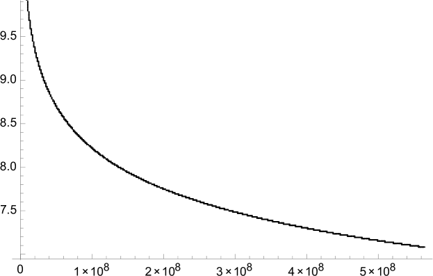
Figure 7. Percentages of Hasse failures: $100\times\frac{\mathcalorig{A}_{\scriptscriptstyle HF}(K)}{\mathcalorig{A}(K)}$ .

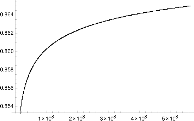
Figure 8. Plot of $\frac{\log{\mathcalorig{A}_{\scriptscriptstyle HF}(K)}}{\log{\mathcalorig{A}(K)}}$.

$R^{2}$ Goodness of Fit: 0.99999359 Correlation Coefficient: 0.99999689 Maximum Error: 0.00015802515 Mean Squared Error: $6.09792\times 10^{-11}$ Mean Absolute Error: $3.4565103\times 10^{-6}$ Table 2. Data on approximation: $\frac{\log{\mathcalorig{A}_{\scriptscriptstyle HF}(K)}}{\log{\mathcalorig{A}(K)}}\sim f(K)$,  $2\times 10^{6}<k<564\times 10^{6}$

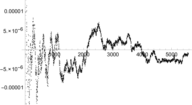
Figure 9. Normalised residuals between $\frac{\log{\mathcalorig{A}_{\scriptscriptstyle HF}(K)}}{\log{\mathcalorig{A}(K)}}$ and prediction $f(K)$: x-axis is  $K/100800$.

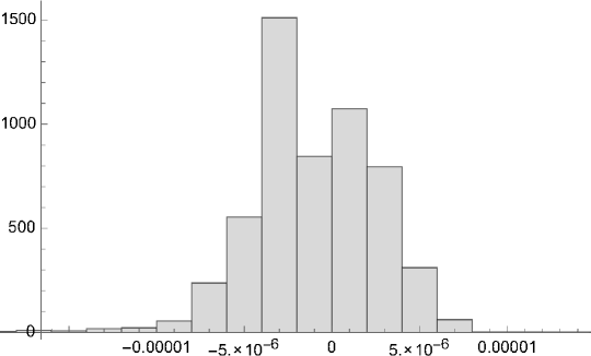
Figure 10. Histogram of residuals above.

Table 3. Percentages of Hasse failures.

$k\leq K$	${\%}$ Hasse failures
100,800	12.97620
10,080,000	9.84888
20,160,000	9.34943
30,240,000	9.05874
40,320,000	8.85229
50,400,000	8.69513
60,480,000	8.56721
70,560,000	8.45991
80,640,000	8.36626
90,720,000	8.28619

$k\leq K$	$\%$ Hasse failures
100,800,000	8.21313
110,880,000	8.14845
120,960,000	8.08844
131,040,000	8.03345
141,120,000	7.98373
151,200,000	7.93721
161,280,000	7.89398
171,360,000	7.85349
181,440,000	7.81481
191,520,000	7.77902

$k\leq K$	$\%$ Hasse failures
201,600,000	7.74513
211,680,000	7.71296
221,760,000	7.68273
231,840,000	7.65369
241,920,000	7.62577
252,000,000	7.59906
262,080,000	7.57319
272,160,000	7.54791
282,240,000	7.52428
292,320,000	7.50153

$k\leq K$	$\%$ Hasse failures
302,400,000	7.47924
312,480,000	7.45807
322,560,000	7.43758
332,640,000	7.41768
342,720,000	7.39828
352,800,000	7.37978
362,880,000	7.36165
372,960,000	7.34364
383,040,000	7.32663
393,120,000	7.30999

$k\leq K$	$\%$ Hasse failures
403,200,000	7.29355
413,280,000	7.27757
423,360,000	7.26198
433,440,000	7.24716
443,520,000	7.23274
453,600,000	7.21817
463,680,000	7.20418
473,760,000	7.19059

$k\leq K$	$\%$ Hasse failures
483,840,000	7.17718
493,920,000	7.16409
504,000,000	7.15137
514,080,000	7.13901
524,160,000	7.12665
534,240,000	7.11460
544,320,000	7.10295
554,400,000	7.09159

In Table 3, we provide a sample of the percentages of the Hasse failures. The data in Table 3 suggests that

$$\mathcalorig{A}_{\scriptscriptstyle HF}(K)\sim C\ K^{0.8875...+\ {\text{o}}(1)}$$

for some constant $C$, at least for $K$ in this range. The error is smaller than $0.1\%$ for $K\geq 10^{7}$ and gets better for larger values of $K$. This is illustrated in Table 4.

We could use $f(K)=1-\frac{C}{\log{K}}+\ldots$ to test for the “positive proportion” case (which we know is false), and use $f(K)=1-\frac{C\log\log{K}}{\log{K}}+\ldots$ for case (2). For our range of $K$, $\log\log K$ is essentially constant and we will not be able to distinguish between these cases satisfactorily. Testing gave a candidate function whose error in approximating is closer to $1\%$, a result much weaker than the one for case (1) above. Moreover, the graph of the normalised residuals (not shown) was far from random.

We do not come to any firm conclusions from these computations as our range of $k$’s may well be too small (since $\log K$ does not grow fast enough), and because the exponent $0.8875...$ is quite close to 1. However, it is still a bit of a surprise how well columns 2 and 3 match in Table 4.

We next consider a slightly different calculation. Recall that we subdivided our large interval into subintervals of length $h=100,800$ (this value was chosen to be a nice integer slightly larger than $\sqrt{K}=23750$). It is interesting to look at the distribution of HF’s within these subintervals. We plot $\frac{1}{h}\left(\mathcalorig{A}_{\scriptscriptstyle HF}((l+1)h)-\mathcalorig{A}_{\scriptscriptstyle HF}(lh)\right)$, the average number of HF’s in the $l$-th subinterval, with $lh\leq K$. The curve in the graph is an approximation, given by $g(x)=0.2353x^{-0.0908047}-46.7396x^{-0.661084}$ (there was no effort made to find “optimal” coefficients in the approximation). The residuals appear random, with the histogram fitting the normal distribution $N(-0.0016,0.0018)$ quite closely.

Table 4. Comparision between Hasse failure count $\mathcalorig{A}_{\scriptscriptstyle HF}(K)$ and the model $\mathcalorig{P}(K)$.

$k$	$\mathcalorig{A}_{\scriptscriptstyle HF}(K)$	$\mathcalorig{P}(K)$	error: $\mathcalorig{E}(K)$%
6,552,000	388,485	388,474	0.00279494
13,104,000	738,402	738,476	-0.0100959
19,656,000	1,074,038	1,074,075	-0.00351784
26,208,000	1,400,385	1,400,458	-0.00526837
32,760,000	1,720,203	1,720,067	0.0078529
39,312,000	2,034,145	2,034,330	-0.00913502
45,864,000	2,343,944	2,344,184	-0.0102605
52,416,000	2,650,338	2,650,290	0.0017743
58,968,000	2,952,994	2,953,142	-0.00502773
65,520,000	3,253,233	3,253,119	0.00349665
72,072,000	3,550,279	3,550,523	-0.00689091
78,624,000	3,845,160	3,845,601	-0.0114887
85,176,000	4,138,458	4,138,557	-0.00241157
91,728,000	4,429,888	4,429,563	0.00732315
98,280,000	4,718,612	4,718,766	-0.00326508
104,832,000	5,006,091	5,006,291	-0.00401399
111,384,000	5,292,241	5,292,251	-0.000204305
117,936,000	5,576,772	5,576,742	0.00052202
124,488,000	5,859,223	5,859,851	-0.0107229
131,040,000	6,140,768	6,141,654	-0.0144272
137,592,000	6,421,657	6,422,220	-0.00876724
144,144,000	6,701,189	6,701,611	-0.00630533
150,696,000	6,979,137	6,979,885	-0.0107173
157,248,000	7,256,456	7,257,091	-0.00876333
163,800,000	7,532,631	7,533,279	-0.00860614
170,352,000	7,807,978	7,808,490	-0.00656096
176,904,000	8,082,302	8,082,764	-0.00572446
183,456,000	8,355,009	8,356,139	-0.0135256
190,008,000	8,627,950	8,628,647	-0.0080886
196,560,000	8,899,431	8,900,322	-0.0100164
203,112,000	9,170,775	9,171,192	-0.00455085
209,664,000	9,440,833	9,441,285	-0.00478836
216,216,000	9,710,721	9,710,626	0.000974181
222,768,000	9,979,756	9,979,240	0.00516595
229,320,000	10,247,890	10,247,150	0.00722142
235,872,000	10,515,262	10,514,376	0.00842309
242,424,000	10,781,980	10,780,939	0.00964957
248,976,000	11,047,893	11,046,859	0.0093601
255,528,000	11,313,674	11,312,152	0.0134518
262,080,000	11,577,887	11,576,836	0.00907272
268,632,000	11,841,388	11,840,928	0.00388283
275,184,000	12104,565	12,104,442	0.00101294

$K$	$\mathcalorig{A}_{\scriptscriptstyle HF}(K)$	$\mathcalorig{P}(K)$	error: $\mathcalorig{E}(K)$%
281,736,000	12,367,646	12,367,393	0.00203978
288,288,000	12,630,282	12,629,796	0.00384661
294,840,000	12,892,179	12,891,662	0.00400262
301,392,000	13,153,376	13,153,006	0.00280671
307,944,000	13,414,178	13,413,839	0.00252140
314,496,000	13,674,773	13,674,173	0.00438484
321,048,000	13,934,649	13,934,018	0.00452291
327,600,000	14,194,163	14,193,386	0.00547096
334,152,000	14,452,782	14,452,286	0.00342712
340,704,000	14,711,231	14,710,729	0.00341123
347,256,000	14,969,227	14,968,723	0.00336506
353,808,000	15,227,250	15,226,278	0.00638342
360,360,000	15,484,481	15,483,402	0.00696817
366,912,000	15,740,411	15,740,103	0.00195186
373,464,000	15,996,468	15,996,391	0.00048054
380,016,000	16,252,525	16,252,271	0.00155736
386,568,000	16,508,096	16,507,753	0.00207456
393,120,000	16,763,273	16,762,843	0.00256364
399,672,000	17,017,822	17,017,548	0.00160994
406,224,000	17,271,602	17,271,874	-0.00157807
412,776,000	17,525,323	17,525,829	-0.00288924
419,328,000	17,778,565	17,779,418	-0.00480173
425,880,000	18,031,595	18,032,648	-0.00584339
432,432,000	18,284,841	18,285,525	-0.00374203
438,984,000	18,537,717	18,538,054	-0.00181802
445,536,000	18,790,012	18,790,240	-0.00121647
452,088,000	19,041,406	19,042,090	-0.00359348
458,640,000	19,292,457	19,293,608	-0.00596736
465,192,000	19,543,623	19,544,799	-0.00602086
471,744,000	19,794,451	19,795,669	-0.00615548
478,296,000	20,045,181	20,046,222	-0.00519473
484,848,000	20,295,253	20,296,462	-0.00596103
491,400,000	20,545,280	20,546,395	-0.00542974
497,952,000	20,794,925	20,796,024	-0.00528918
504,504,000	21,044,290	21,045,355	-0.00506101
511,056,000	21,293,257	21,294,390	-0.00532190
517,608,000	21,541,991	21,543,134	-0.00530773
524,160,000	21,790,444	21,791,591	-0.00526622
530,712,000	22,038,418	22,039,765	-0.00611405
537,264,000	22,286,350	22,287,659	-0.00587756
543,816,000	22,534,130	22,535,278	-0.00509679
550,368,000	22,782,046	22,782,624	-0.00254092

Finally we include data on the distribution of the number of orbits $\mathfrak{h}(k)$ with generic $k\leq K$ where $K=10^{7}$. A sample of fundamental sets together with the corresponding class numbers $\mathfrak{h}(k)$ obtained using Theorem 1.1(i) is given in Table LABEL:funsettable. The data on the distribution of these class numbers is given in Table 6 and Fig. 14. Here, $\mathfrak{n}(h)=\mathfrak{n}_{K}(h)$ is the number of occurrences of $h=\mathfrak{h}(k)$ with $k$ running through generic integers in $[1,K]$. Our count also includes the number of Hasse failures, denoted by $\mathfrak{n}(0)$. Since $\mathfrak{n}(0)$ grows with $K$, we normalize our counts and consider the distribution of $\frac{\mathfrak{n}(h)}{\mathfrak{n}(0)}$. We find that this quantity appears to behave like the graph of $e^{-\sqrt{h+1}}$. If so, this suggests that $\frac{\mathfrak{n}(h+1)}{\mathfrak{n}(h)}\sim 1-\frac{1}{2}h^{-\frac{1}{2}}$ as $h\rightarrow\infty$. This is roughly consistent with the data in the second column of Table 6, for which with $h=21$ we have $\frac{\mathfrak{n}(h+1)}{\mathfrak{n}(h)}=0.88921$ while $1-\frac{1}{2}h^{-\frac{1}{2}}=0.89089$. By Lemma 7.2, the average value of $\mathfrak{h}(k)$ with $0\leq k\leq K$ has size about $(\log K)^{2}$. Since $\mathfrak{n}(0)$ has size a power of $K$, the data (at least in this short range for $K$) suggests that the maximal value of $\mathfrak{h}(k)$ is probably a power of $\log K$ , or at worst $\mathfrak{h}(k)\ll_{\epsilon}k^{\epsilon}$, for $\epsilon>0$ (the maximum value for $\mathfrak{h}(k)$ in our data was 131). As mentioned in the introduction, the best we know is $\mathfrak{h}(k)\ll_{\varepsilon}k^{\frac{1}{3}+\varepsilon}$.

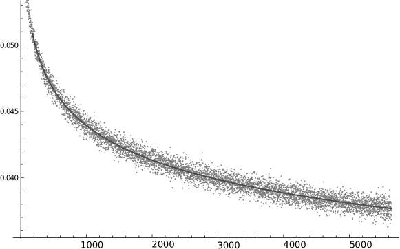
Figure 11. Hasse failures in subintervals. 

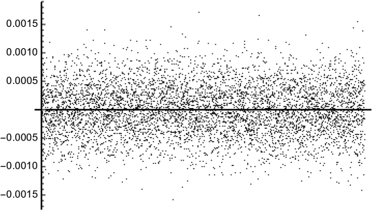
Figure 12. Hasse failures in subintervals residuals.

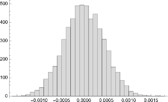
Figure 13. Hasse failures in subintervals: residuals histogram and probability plot.

Table 5. Sample fundamental sets, $(-u_{1},u_{2},u_{3})$

$k$	$\mathfrak{h}(k)$	$(u_{1},u_{2},u_{3})$
54	1	(3, 3, 3)
70	1	(3, 3, 4)
88	1	(3, 3, 5)
108	1	(3, 3, 6)
133	1	(3, 4, 6)
154	1	(3, 3, 8)
166	1	(4, 5, 5)
188	1	(3, 5, 7)
189	1	(3, 6, 6)
214	1	(3, 4, 9)
236	1	(5, 5, 6)
254	1	(3, 7, 7)
270	1	(3, 3, 12)
304	1	(3, 3, 13)
329	2	(3, 8, 8), (4, 4, 11)
341	1	(4, 5, 10)
358	1	(3, 5, 12)
378	1	(3, 3, 15)
412	1	(5, 6, 9)
414	1	(3, 9, 9)
430	1	(3, 4, 15)
446	1	(5, 5, 11)
448	1	(3, 6, 13)
460	2	(3, 3, 17), (3, 9, 10)
473	2	(3, 4, 16), (5, 8, 8)
494	2	(4, 7, 11), (5, 5, 12)
502	1	(4, 9, 9)
504	1	(3, 3, 18)
518	1	(3, 4, 17)
532	1	(6, 6, 10)
540	1	(3, 6, 15)
553	1	(4, 8, 11)
558	1	(3, 9, 12)
566	1	(4, 5, 15)
616	1	(4, 10, 10)
664	1	(3, 9, 14)
665	2	(3, 4, 20), (4, 8, 13)
668	2	(3, 10, 13), (6, 7, 11)
684	1	(6, 9, 9)
693	1	(3, 6, 18)
700	1	(3, 3, 22)
713	2	(3, 8, 16), (5, 8, 12)
718	1	(3, 4, 21)
…	…	…
…	…	…
9230	3	(3, 28, 59), (7, 17, 52), (11, 25, 28)
9234	2	(3, 15, 75), (9, 9, 63)
9253	3	(3, 42, 44), (8, 9, 66), (12, 18, 35)
9260	9	(3, 7, 86), (3, 19, 70), (3, 29, 58), (5, 19, 58), (5, 31, 42)
		(6, 23, 47), (7, 31, 33),(9, 13, 53), (9, 22, 37)
9261	1	(6, 15, 60)
9268	1	(6, 32, 36)
9288	2	(3, 30, 57), (6, 12, 66)
9289	1	(3, 24, 64)
9296	1	(10, 11, 55)
9302	3	(4, 21, 61), (5, 9, 76), (11, 19, 36)
9304	5	(3, 13, 78), (9, 14, 51), (9, 27, 31), (13, 18, 33), (14, 21, 27)
9308	3	(5, 27, 47), (9, 11, 58), (10, 23, 33)
9310	3	(3, 3, 92), (3, 20, 69), (4, 13, 73)
9313	1	(4, 24, 57)
9317	2	(4, 6, 85), (4, 34, 45)
9322	2	(5, 24, 51), (9, 15, 49)
9329	2	(7, 8, 72), (8, 28, 33)
9353	3	(4, 36, 43), (8, 12, 59), (8, 29, 32)
9358	4	(3, 21, 68), (9, 23, 36), (12, 13, 45), (12, 21, 31)
9368	3	(3, 14, 77), (7, 21, 46), (13, 21, 29)
9373	4	(3, 6, 88), (4, 38, 41), (11, 22, 32), (18, 18, 25)
9380	7	(3, 34, 53), (4, 22, 60), (6, 20, 52), (8, 10, 64), (8, 24, 38)
		(10, 24, 32), (15, 17, 31)
9388	3	(6, 9, 73), (6, 17, 57), (9, 19, 42)
9405	1	(3, 18, 72)
9414	3	(3, 9, 84), (3, 36, 51), (9, 21, 39)
9416	2	(4, 30, 50), (5, 29, 45)
9430	2	(3, 15, 76), (12, 15, 41)
9436	2	(6, 25, 45), (10, 25, 31)
9446	1	(11, 20, 35)
9449	2	(4, 16, 69), (8, 16, 51)
9450	1	(3, 39, 48)
9454	11	(3, 7, 87), (4, 11, 77), (4, 23, 59), (4, 31, 49), (7, 12, 63),
		(7, 17, 53), (7, 28, 37), (11, 23, 31), (13, 13, 43), (15, 20, 27)
		(17, 17, 28)
9468	1	(3, 42, 45)
9470	4	(3, 43, 44), (5, 7, 81), (5, 12, 71), (17, 21, 23)
9484	2	(3, 5, 90), (9, 13, 54)
9493	5	(3, 30, 58), (4, 27, 54), (6, 12, 67), (6, 14, 63), (6, 23, 48)
9494	1	(7, 29, 36)
9500	8	(3, 13, 79), (5, 9, 77), (5, 10, 75), (5, 31, 43), (6, 13, 65)
		(10, 13, 51), (10, 27, 29), (13, 23, 27)
9504	3	(3, 3, 93), (6, 21, 51), (12, 12, 48)
9520	2	(3, 31, 57), (13, 15, 39)
9532	1	(15, 21, 26)
9538	1	(5, 27, 48)

Table 6. Distribution of $\mathfrak{h}(k)$, generic $k\leq 10^{7}$.

$\mathfrak{h}(k)$	$\mathfrak{n}(\mathfrak{h}(k))$ occurrences
0	574,778
1	423,094
2	346,019
3	259,787
4	202,111
5	157,726
6	124,744
7	100,431
8	81,243
9	66,794
10	54,942
11	45,898
12	38,719
13	32,886
14	28,001
15	23,954
16	20,930
17	17,932
18	15,970
19	13,748
20	12,105
21	10,434

$s$	$\mathfrak{n}(s+1)/\mathfrak{n}(s)$
0	0.7361
1	0.81783
2	0.750788
3	0.777987
4	0.780393
5	0.790891
6	0.805097
7	0.808943
8	0.822151
9	0.822559
10	0.83539
11	0.843588
12	0.84935
13	0.851457
14	0.855469
15	0.873758
16	0.856761
17	0.890587
18	0.860864
19	0.880492
20	0.861958
21	0.888921

We end this Section with some basic Conjectures concerning the class numbers $\mathfrak{h}(k)$. These are suggested by our theoretical results as well as our more refined numerical findings.

Conjecture 10.1.

For any $\varepsilon>0$

$$\mathfrak{h}(k)\ll_{\varepsilon}\ |k|^{\varepsilon}.$$

Conjecture 10.2.

The number of Hasse failures for $0\leq k\leq K$ satisfies

$$\big{|}\left\{0\leq k\leq K:\mathfrak{h}(k)=0\ \text{and}\ k\ \text{admissible}\ \right\}\big{|}\sim C_{0}K^{\theta},$$

for some $C_{0}>0$ and some $\frac{1}{2}<\theta<1$.

More generally, for $t\geq 1$

$$\big{|}\left\{0\leq k\leq K:\mathfrak{h}(k)=t\ \text{\ }\right\}\big{|}\sim C_{t}K^{\theta},$$

with $C_{t}>0$.

The values of $C_{t}$ above are illustrated in Fig. 14, suggesting an exponential decay in $t$.

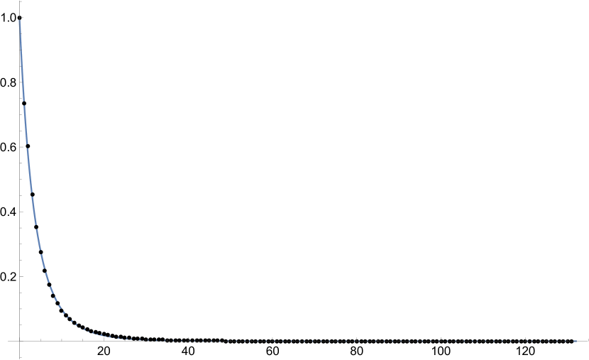
Figure 14. Occurences of relative number of orbits: $\mathfrak{n}(\mathfrak{h}(k))/\mathfrak{n}(0)$,
generic $k\leq 10^{7}$. Approximation curve $\mathfrak{n}(h)=\mathfrak{n}(0)(6.86293+4.62621h$ $+0.0576149h^{2})e^{-1.92905\sqrt{h+1}}$.

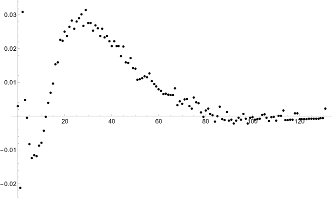
Figure 15. Residuals to Fig. 14.

Appendix

The appendix consists of (A) a discussion of invariants of affine cubic forms referred to in the Introduction, and (B) computation of local masses $\delta_{p}$, for primes $p\geq 2$ (with some details omitted); their structure is used in the proofs in Section 9.

Appendix A Arithmetic invariants of affine cubic forms.

A number of invariants of $f$ as an element of the unique factorization domain $R=\mathbb{Q}[x_{1},x_{2},\ldots,x_{n}]$, enter into the study of the values assumed by such an affine cubic form $f$. The first is the $\mathcal{h}$-invariant from [DL64]: $\mathcal{h}(f)$ is the minimal integer $h$ for which

(A.1) $$f_{0}=L_{1}Q_{1}+L_{2}Q_{2}+\ldots+L_{h}Q_{h},$$

where the $L_{j}$’s are homogeneous linear and the $Q_{j}$’s are homogeneous quadratic members of $R$; equivalently $n-\mathcal{h}(f)$ is the dimension of the largest $\mathbb{Q}$-linear subspace contained in $W_{0}=\left\{{\bf x}:f_{0}({\bf x})=0\right\}$, the linear space given by $L_{1}=L_{2}=\ldots=L_{h}=0$. Note that $\mathcal{h}(f)=1$ iff $f_{0}$ is reducible in $R$, and in this case $W_{0}$ contains a rational hypersurface.

Closely related are the $\mathbb{Q}$-invariants $\mathcal{l}(f)$ and $\mathcal{q}(f)$ defined as the dimensions of the largest $\mathbb{Q}$-affine linear subspaces $U_{\mathcal{l}}$ and $U_{\mathcal{q}}$ of $\mathbb{A}^{n}$ on which the restriction of $f$ to $U_{\mathcal{l}}$ is linear (non-constant) and to $U_{\mathcal{q}}$ is quadratic. So, $\mathcal{l}(f)$ and $\mathcal{q}(f)$ lie in $[0,n-1]$. Of particular interest to us is that

(A.2) $$\mathcal{h}(f)=1\quad\text{iff}\quad\mathcal{q}(f)=n-1.$$

The group $\text{Aff}_{n}(\mathbb{Z})$ consisting of integral affine linear maps ${\bf x}\to A{\bf x}+{\bf b}$ with $A\in\text{GL}_{n}(\mathbb{Z})$ and ${\bf b}\in\mathbb{Z}^{n}$, acts on the integral cubic polynomials by a change of variable. The arithmetic invariants as well as the diophantine questions concerning $V_{k,f}(\mathbb{Z})$ are all preserved by this action. On the leading homogeneous cubic term $f_{0}$, the action is that of $\text{GL}_{n}(\mathbb{Z})$, which has been well studied in terms of its invariants. With these fixed, there are finitely many $\text{GL}_{n}(\mathbb{Z})$ orbits, see [BS15] for a recent discussion of the case $n=3$, which is our interest. In this case the vector space of $f_{0}$’s is 10-dimensional and it’s quotient by $SL_{3}$ is 2-dimensional, given by the Aronhold invariants $I$ and $J$. The vector space of $f$’s is 20-dimensional and its quotient by $\text{Aff}_{3}$ is 9-dimensional. The invariants for this action up to the additive constant term and at a generic point are $I(f_{0})$, $J(f_{0})$ together with the 6-dimensional vector space associated with the homogeneous quadratic part of $f$

We end with some examples of affine cubic forms and their invariants.

1. $S({\bf x})=x_{1}^{3}+x_{2}^{3}+x_{3}^{3}$, $\mathcal{h}(S)=3$, $\mathcal{l}(S)=\mathcal{q}(S)=0$;

2. $M({\bf x})=x_{1}^{2}+x_{2}^{2}+x_{3}^{2}-x_{1}x_{2}x_{3}$, $\mathcal{h}(M)=1$, $\mathcal{l}(M)=0$, $\mathcal{q}(M)=2$;

3. $T({\bf x})=x_{1}x_{2}x_{3}+x_{1}+x_{2}$ (perhaps the mildest perturbation of the fully split form $x_{1}x_{2}x_{3}$), $\mathcal{h}(M)=1$, $\mathcal{l}(M)=\mathcal{q}(M)=2$ (the restriction of $T$ to $x_{3}=0$ is linear). From the last it follows that $\mathfrak{v}_{T}(k)=|V_{k,T}(\mathbb{Z})|=\infty$; however $T$ is not perfect or even almost perfect since $V_{k,T}(\mathbb{Z})$ is not Zariski dense in $V_{k,T}$ for $k\neq 0$.

4. $P({\bf x})=x_{1}x_{2}x_{3}+(x_{1}-1)Q_{1}({\bf x})+(x_{2}-1)Q_{2}({\bf x})$, with $Q_{1}$, $Q_{2}$ generic quadratics. Then, $\mathcal{l}(P)=\mathcal{q}(P)=1$ (with $x_{1}=x_{2}=1$ giving the line $U_{\mathcal{l}}$). In particular, $V_{k,P}(\mathbb{Z})\neq\emptyset$ for every $k$. We expect that $P$ is full.

Appendix B Analysis of the local masses.

B.1. Computation of $\delta_{p}(k)$ for odd primes.

For any integer $k$ and prime $p\geq 3$, we determine

$$\delta_{p}(k)=\lim_{l\to\infty}\ |V_{k}(\mathbb{Z}/\;p^{l}\mathbb{Z})|\;p^{-2l}\ .$$

Define

(B.1) $$N_{l}(k)=p^{-3l}\sideset{}{{}^{*}}{\sum}_{b\ (\text{mod}\ p^{l})}\ \sum_{{\bf x}\ (\text{mod}\ p^{l})}\ e\left(\frac{f({\bf x})-k}{p^{l}}b\right)\ ,$$

where ${\bf x}=(x_{1},x_{2},x_{3})$, $f({\bf x})=x_{1}^{2}+x_{2}^{2}+x_{3}^{2}-x_{1}x_{2}x_{3}$ and the asterisk denotes a sum over those $b$’s not divisible by $p$. Then one has

(B.2) $$\delta_{p}(k)=1+\sum_{l=1}^{\infty}N_{l}(k)\ .$$

In what follows, we analyze the case $l\geq 2$ (the case $l=1$ is determined by Lemma 6.4). For $p\geq 3$ one has

(B.3) $$N_{l}(k)=p^{-3l}\sideset{}{{}^{*}}{\sum}_{b\ (\text{mod}\ p^{l})}\ e\left(\frac{4(4-k)}{p^{l}}b\right)\sum_{{\bf x}}\ e\left(\frac{(2x_{3}-x_{1}x_{2})^{2}-(x_{1}^{2}-4)(x_{2}^{2}-4)}{p^{l}}b\right)\ .$$

Making a change of variable shows that the inner sum over ${\bf x}$ is

(B.4) $$\sum_{u}\sum_{x_{1},x_{2}}\ e\left(\frac{bu^{2}}{p^{l}}\right)\ e\left(\frac{-b(x_{1}^{2}-4)(x_{2}^{2}-4)}{p^{l}}\right)=S(b;p^{l})\sum_{x}\ e\left(\frac{4b(x^{2}-4)}{p^{l}}\right)\overline{S\left(b(x^{2}-4);p^{l}\right)}\ ,$$

where for $q\geq 1$ we put

(B.5) $$S(b;q)=\sum_{r\ ({\rm mod}\ q)}e\left(\frac{br^{2}}{q}\right).$$

Using properties of the Gauss sum, we get

Proposition B.1.

For $p\geq 3$ we have

1. $$N_{1}(k)=\chi(k-4)\left[3+\chi(k)\right]\frac{1}{p}+\frac{1}{p^{2}}\ ;$$

2. if $l\geq 3$ is odd,

   $$N_{l}(k)=\left\{\begin{array}[]{ll}4p^{-\frac{1}{2}(l+1)}\chi\left(\frac{k-4}{p^{l-1}}\right)&\text{if}\ \ p^{l-1}|(k-4),\\ p^{-\frac{1}{2}(l+1)}\chi\left(\frac{k}{p^{l-1}}\right)&\text{if}\ \ p^{l-1}|k,\\ \quad 0&\text{otherwise}\ ;\end{array}\right.$$

3. if $l\geq 2$ is even, then

   $$N_{l}(k)=\left\{\begin{array}[]{ll}-p^{-\frac{l+2}{2}}\left\{4\eta_{l-1}(k-4)+\eta_{l-1}(k)\right\}&\text{if}\ \ p^{l-1}||k(k-4),\\ p^{-\frac{l}{2}}\left(1-\frac{1}{p}\right)\left\{4\eta_{l}(k-4)+\eta_{l}(k)\right\}&\text{if}\ \ p^{l}|k(k-4),\\ \quad 0&\text{otherwise},\end{array}\right.$$

   where we define $\eta_{l}(m)=1$ if $p^{l}|m$ and is zero otherwise;

where $\chi(b)$ denotes the Legendre symbol $\left(\frac{b}{p}\right)_{L}$.

To compute $\delta_{p}(k)$ for $p\geq 3$ in (B.2), we write $\delta_{p}(k)=1+N_{1}(k)+\mathfrak{S}_{p}(k)$. Define $\mu\geq 0$ by $p^{\mu}||k(k-4)$. By Prop. B.1, $\mu=0$ implies $N_{l}(k)=0$ for $l\geq 2$, so that we have $\mathfrak{S}_{p}(k)=0$ for this case. For $\mu\geq 1$, we have $p^{\mu}||(k-4\beta)$, with $\beta=0$ or $1$. Then we combine Prop. B.1 in (B.2), to get

(B.6) $$\mathfrak{S}_{p}(k)=4^{\beta}\times\left\{\begin{array}[]{ll}p^{-1}-p^{-\frac{1}{2}(\mu+1)}-p^{-\frac{1}{2}(\mu+3)}&\text{if}\ \ 2\nmid\mu\ ,\\ p^{-1}-p^{-\frac{\mu}{2}-1}\left(1-\chi\left(\frac{k-4\beta}{p^{\mu}}\right)\right)&\text{if}\ \ 2|\mu\ .\end{array}\right.$$

In particular, we see that if $\mu=1$, then $\mathfrak{S}_{p}(k)=-4^{\beta}p^{-2}$ while if $\mu\geq 2$ then $\mathfrak{S}_{p}(k)=4^{\beta}p^{-1}+O(p^{-2})$.

Combining (B.6) with Prop. B.1(a) in (B.2) gives

Proposition B.2.

For $p\geq 3$, suppose $p^{\mu}||k(k-4)$ with $\mu\geq 0$. We have

1. if $\mu=0$, then $\delta_{p}(k)=1+\chi(k-4)\left[3+\chi(k)\right]\frac{1}{p}+\frac{1}{p^{2}}$ ;

2. if $p||k$, then $\delta_{p}(k)=1+3\chi(-1)\frac{1}{p}$ ;

3. if $p||(k-4)$, then $\delta_{p}(k)=1-\frac{3}{p^{2}}$ ;

4. if $\mu\geq 2$ and $p|k$, then

   $$\delta_{p}(k)=1+\left\{\begin{array}[]{ll}\left(1+3\chi(-1)\right)p^{-1}+p^{-2}-p^{-\frac{1}{2}(\mu+1)}-p^{-\frac{1}{2}(\mu+3)}&\text{if}\ \ 2\nmid\mu\ ,\\ \left(1+3\chi(-1)\right)p^{-1}+p^{-2}-p^{-\frac{\mu}{2}-1}\left(1-\chi\left(\frac{k}{p^{\mu}}\right)\right)&\text{if}\ \ 2|\mu\ ;\end{array}\right.$$

5. if $\mu\geq 2$ and $p|(k-4)$, then

   $$\delta_{p}(k)=1+\left\{\begin{array}[]{ll}4p^{-1}+p^{-2}-4p^{-\frac{1}{2}(\mu+1)}-4p^{-\frac{1}{2}(\mu+3)}&\text{if}\ \ 2\nmid\mu\ ,\\ 4p^{-1}+p^{-2}-4p^{-\frac{\mu}{2}-1}\left(1-\chi\left(\frac{k}{p^{\mu}}\right)\right)&\text{if}\ \ 2|\mu\ .\end{array}\right.$$

Remark B.3.

The case (b) shows that $\delta_{3}(k)=0$ if $k\equiv 3$ or $6$ (mod $9$), while case (a) and (d) shows that $\delta_{3}(k)>0$ otherwise.

B.2. Local factors associated with $V_{a_{1},a_{2}}$, odd primes.

We next state (without details) the analogous results for the density function $\delta_{p}(a_{1},a_{2})$ in (9.19) for the surface $V_{a_{1},a_{2}}$ in (9.18). Recalling the properties in (9.26) and (9.27), since $p$ is odd, completing the square gives us

(B.7) $$N_{l}(a_{1},a_{2})=p^{-3l}\sideset{}{{}^{*}}{\sum}_{b\ (\text{mod}\ p^{l})}e\left(4b\frac{D_{a_{1}}-D_{a_{2}}}{p^{l}}\right)\overline{S(bD_{a_{1}};p^{l})}S(bD_{a_{2}};p^{l})\ .$$

Again, using properties of the Gauss sums gives us

Proposition B.4.

Let $a_{1}\neq a_{2}$ be fixed, and let $p\geq 3$.

1. Suppose $p\nmid D_{a_{1}}D_{a_{2}}\left(D_{a_{1}}-D_{a_{2}}\right)$. Then

   $$N_{l}(a_{1},a_{2})=\left\{\begin{array}[]{ll}-\frac{\chi\left(D_{a_{1}}D_{a_{2}}\right)}{p^{2}}&\text{if}\ \ l=1,\\ 0&\text{otherwise}\ .\end{array}\right.$$

2. Suppose $p\nmid D_{a_{1}}D_{a_{2}}$ and $p^{\mu}||\left(D_{a_{1}}-D_{a_{2}}\right)$ with $\mu\geq 1$. Then

   $$N_{l}(a_{1},a_{2})=\left\{\begin{array}[]{ll}\frac{1}{p^{l}}\left(1-\frac{1}{p}\right)&\text{if}\ l\leq\mu,\\ -p^{-\mu-2}&\text{if}\ l=\mu+1,\\ 0&\text{otherwise}\ .\end{array}\right.$$

3. Suppose $p^{\alpha}||D_{a_{1}}$ but $\ p\nmid D_{a_{2}}$ with $\alpha\geq 1$. Then

   $$N_{l}(a_{1},a_{2})=\left\{\begin{array}[]{ll}p^{-1}&\text{if}\ \ l=1,\\ 0&\text{otherwise}\ .\end{array}\right.$$

4. Suppose $p^{\eta_{1}}||D_{a_{1}}$, $p^{\eta_{2}}||D_{a_{2}}$ and $p^{\mu}||\left(D_{a_{1}}-D_{a_{2}}\right)$ with $\eta_{1}$,$\eta_{2}$ and $\mu\geq 1$ . Putting $\eta=\min{(\eta_{1},\eta_{2})}$ gives us

   $$N_{l}(a_{1},a_{2})=\left\{\begin{array}[]{ll}\left(1-\frac{1}{p}\right)&\text{if}\ \ 1\leq l\leq\eta\ ,\\ p^{-1}&\text{if}\ \ l=\eta+1,\ \eta_{1}\neq\eta_{2}\ ,\\ -p^{-\eta-2}\chi\left(\frac{D_{a_{1}}}{p^{\eta}}\right)\chi\left(\frac{D_{a_{2}}}{p^{\eta}}\right)&\text{if}\ \ l=\eta+1,\ \eta_{1}=\eta_{2}\leq\mu\ ,\\ 0&\text{otherwise}\ .\end{array}\right.$$

It then follows that

Proposition B.5.

Let $a_{1}\neq a_{2}$ be fixed, and let $p\geq 3$.

1. Suppose $p\nmid D_{a_{1}}D_{a_{2}}\left(D_{a_{1}}-D_{a_{2}}\right)$. Then

   $$\delta_{p}(a_{1},a_{2})=1-\frac{\chi\left(D_{a_{1}}D_{a_{2}}\right)}{p^{2}}\ .$$

2. Suppose $p\nmid D_{a_{1}}D_{a_{2}}$ and $p^{\mu}||\left(D_{a_{1}}-D_{a_{2}}\right)$ with $\mu\geq 1$. Then

   $$\delta_{p}(a_{1},a_{2})=\left(1+\frac{1}{p}\right)\left(1-\frac{1}{p^{\mu+1}}\right)\ .$$

3. Suppose $p|D_{a_{1}}D_{a_{2}}$ but $p\nmid\left(D_{a_{1}}-D_{a_{2}}\right)$. Then

   $$\delta_{p}(a_{1},a_{2})=\left(1+\frac{1}{p}\right)\ .$$

4. Suppose $p^{\eta_{1}}||D_{a_{1}}$, $p^{\eta_{2}}||D_{a_{2}}$ and $p^{\mu}||\left(D_{a_{1}}-D_{a_{2}}\right)$ with $\eta_{1}$,$\eta_{2}$ and $\mu\geq 1$ . Putting $\eta=\min{(\eta_{1},\eta_{2})}$ gives us

   $$\delta_{p}(a_{1},a_{2})=\left\{\begin{array}[]{ll}(1+\eta)-\frac{\eta-1}{p}&\text{if}\ \ \eta_{1}\neq\eta_{2}\ ,\\ (1+\eta)-\frac{\eta}{p}-\frac{1}{p^{2}}\chi\left(\frac{D_{a_{1}}}{p^{\eta}}\right)\chi\left(\frac{D_{a_{2}}}{p^{\eta}}\right)&\text{if}\ \ \eta_{1}=\eta_{2}=\mu\ ,\\ (1+\eta)-\frac{\eta-1}{p}-\frac{1}{p^{\mu-\eta+1}}\left(1+\frac{1}{p}\right)&\text{if}\ \ \eta_{1}=\eta_{2}<\mu\ .\end{array}\right.$$

Remark B.6.

If $a_{1}=a_{2}=a$ and $p\geq 3$, one can deduce the result for $\delta_{p}(a,a)$ from parts (c) and (d) above, with $\mu\to\infty$, giving

1. if $p\nmid D_{a}$, then $\delta_{p}(a,a)=1+p^{-1}$ , and

2. if $p^{\eta}||D_{a}$ with $\eta\geq 1$, then $\delta_{p}(a,a)=(1+\eta)-\frac{\eta-1}{p}$ .

B.3. The even local factor $\delta_{2}(k)$.

Since the analysis here is a bit more delicate, we provide some additional details. Let $l\geq 0$ and define $F_{l}(c)=\sum_{x\ \text{mod}\ 2^{l}}\ e\left(\frac{cx^{2}}{2^{l}}\right)\$. Recall the three primitive real characters modulo powers of two: $\chi_{4}$ modulo 4, $\chi_{8}$ and $\chi_{4}\chi_{8}$ modulo 8, where

$$\chi_{4}(x)=\left(\frac{-4}{x}\right)_{\text{J}}=\left\{\begin{array}[]{ll}\ 1&\text{if}\ \ x\equiv 1\ \text{mod}\ 4\ ,\\ -1&\text{if}\ \ x\equiv 3\ \text{mod}\ 4\ ,\\ \ 0&\ \text{otherwise}\ ,\end{array}\right.$$

and

$$\chi_{8}(x)=\left(\frac{8}{x}\right)_{\text{J}}=\left\{\begin{array}[]{ll}\ 1&\text{if}\ \ x\equiv\pm 1\ \text{mod}\ 8\ ,\\ -1&\text{if}\ \ x\equiv\pm 3\ \text{mod}\ 8\ ,\\ \ 0&\ \text{otherwise}\ .\par\end{array}\right.$$

For $l\geq 1$ we define $\omega_{l}(k)$ to be 1 if $2^{l}|k$ and 0 otherwise; if $l\leq 0$, we define $\omega_{l}(k)$ to be 1 always. Given a term $\omega_{l}(k)$, we define $\hat{k}=\frac{k}{2^{l}}$. While $\omega_{l}(k)=\omega_{l}(-k)$, the corresponding “hat” function is not the same, and the appropriate choice is determined by the $\omega$-function.

We have

Lemma B.7.

Define $\theta\geq 0$ so that $2^{\theta}||c$. We have

1. if $\theta\geq l$, $F_{l}(c)=2^{l}$ ;

2. if $\theta=l-1$, $F_{l}(c)=0$ ;

3. if $l\geq 2$ and $2\nmid c$, then $F_{l}(c)=2^{\frac{l}{2}}\chi_{8}(c)^{l}\left[1+\chi_{4}(c)i\right]$ ;

4. if $l\geq 3$ and $1\leq\theta\leq l-2$, we have

   $$F_{l}(c)=2^{\frac{l+\theta}{2}}\chi_{8}\left(\frac{c}{2^{\theta}}\right)^{l+\theta}\left[1+\chi_{4}\left(\frac{c}{2^{\theta}}\right)i\right]\ ;$$

5. for $l\geq 1$ and $q\in\mathbb{Z}$,

   $$\sideset{}{{}^{*}}{\sum}_{b\ (\text{mod}\ 2^{l})}\ e\left(\frac{qb}{2^{l}}\right)F_{l}(b)=\omega_{l-3}(q)\ 2^{\frac{3(l-1)}{2}}\cos\left(\frac{\hat{q}+1}{4}\pi\right)[1+(-1)^{l+\hat{q}}]\ ,$$

   where $\hat{q}=\frac{q}{2^{l-3}}$, and the sum over $b$ runs through odd numbers.

Lemma B.8.

For any $b$ and $l\geq 0$, put

$$Q_{l}(b;a)=\sum_{x_{1},x_{2}\ (\text{mod}\ 2^{l})}\ e\left(b\frac{x_{1}^{2}+x_{2}^{2}-ax_{1}x_{2}}{2^{l}}\right)\ .$$

1. If $2|a$, then $Q_{l}(b;a)=F_{l}(b)\overline{F_{l}\left(b(\frac{a^{2}}{4}-1)\right)}$,

2. If $2\nmid ab$, then $Q_{l}(b;a)=(-2)^{l}$.

We now compute $N_{l}(k)$ given in (B.1) with $p=2$, where the sum over $b$ runs through odd numbers. It will be convenient to compute $N_{l}(k)$ for some small values and we give it as

Lemma B.9.

1. $N_{0}(k)=1$ ;

2. $N_{1}(k)=\frac{1}{4}(-1)^{k}$ ;

3. $N_{2}(k)=\frac{1}{4}\cos(k\frac{\pi}{2})+\frac{3}{4}\sin(k\frac{\pi}{2})$ ;

4. $$N_{3}(k)=\left\{\begin{array}[]{ll}\frac{3}{4}(-1)^{\frac{k+3}{4}}&\text{if}\ \ k\equiv 1\ \text{mod}\ 4,\\ \quad 0&\text{otherwise}\ .\end{array}\right.$$

For $l\geq 4$, we have

(B.8) $$N_{l}(k)=2^{-3l}\sideset{}{{}^{*}}{\sum}_{b\ (\text{mod}\ 2^{l})}\ e\left(-\frac{kb}{2^{l}}\right)\sum_{a\ (\text{mod}\ 2^{l})}\ e\left(\frac{ba^{2}}{2^{l}}\right)Q_{l}(b;a)\ .$$

Using the lemmas above, we conclude

Lemma B.10.

1. If $k$ is odd and $l\geq 4$, $N_{l}(k)=0$ ;

2. if $l=4$ then $N_{4}(k)=0$ unless $4|k$, in which case

   $$N_{4}(k)=\left\{\begin{array}[]{ll}\frac{1}{2}\chi_{4}\left(\frac{k}{4}\right)&\text{if}\ \ 4||k\ ,\\ \\ \ \frac{1}{4}(-1)^{\frac{k}{8}+1}&\text{if}\ \ 8|k\ ;\end{array}\right.$$

3. if $l=5$, $N_{5}(k)=0$ unless $8|k$, in which case $N_{5}(k)=\frac{3}{4}\chi_{4}\left(\frac{k}{8}\right)$ ;

4. if $l\geq 6$, define ${\hat{k}}=\frac{k}{2^{l-3}}$ or $\frac{4-k}{2^{l-3}}$. Then, $N_{l}(k)=0$ unless ${\hat{k}}\in\mathbb{Z}$, in which case

   $$N_{l}(k)=\left\{\begin{array}[]{ll}-2^{-\frac{l+1}{2}}\cos\left(\frac{{\hat{k}}+1}{4}\pi\right)\left[1+(-1)^{l+{\hat{k}}}\right]&\text{if}\ \ 2^{l-3}|k\ ,\\ \\ 2^{\min(3,\;l-5)-\frac{l+1}{2}}\cos\left(\frac{{\hat{k}}+1}{4}\pi\right)\left[1+(-1)^{l+{\hat{k}}}\right]&\text{if}\ \ 2^{l-3}|(k-4)\ .\end{array}\right.$$

Remark B.11.

Note that for odd $w$, $\cos\left(\frac{w+1}{4}\pi\right)=\frac{1}{2}\chi_{8}(w)\left(1-\chi_{4}(w)\right)=\frac{1}{2}\left(\left(\frac{8}{w}\right)_{\text{J}}-\left(\frac{-8}{w}\right)_{\text{J}}\right)$.

Combining Lemmas B.9 and B.10 gives us

Proposition B.12.

Suppose $k\neq 0$ or $4$. Let $\delta_{2}(k)$ denote the mass at $p=2$. Then $\delta_{2}(k)=0$ only when $k\equiv 3\ ({\text{m}od}\ 4)$. Otherwise $\delta_{2}(k)\geq\frac{3}{4}$. More precisely,

1. If $k$ is odd then

   $$\delta_{2}(k)=\frac{3}{4}\left(1+\chi_{4}(k)\right)\left(2-\chi_{8}(k)\right)\ ;$$

2. if $2||k$, then $\delta_{2}(k)=1$ ;

3. if $4||k$, define $\eta\geq 3$ with $2^{\eta}||(k-4)$, and put $4-k=2^{\eta}w$ with $w$ odd.

   1. if $\eta\geq 6$ is even, $\delta_{2}(k)=\frac{13}{4}-2^{-\frac{\eta-6}{2}}-\left(\frac{-4}{w}\right)_{{\rm J}}2^{-\frac{\eta-4}{2}}+\left(\left(\frac{8}{w}\right)_{{\rm J}}-\left(\frac{-8}{w}\right)_{{\rm J}}\right)2^{-\frac{\eta-2}{2}}$ ,

   2. if $\eta\geq 7$ is odd, $\delta_{2}(k)=\frac{13}{4}-2^{-\frac{\eta-6}{2}}+(-1)^{w}2^{-\frac{\eta-5}{2}}$ ,

   3. if $\eta=3$, $\delta_{2}(k)=1$ ,

   4. if $\eta=4$, $\delta_{2}(k)=2+\frac{1}{4}\left(\left(\frac{8}{w}\right)_{{\rm J}}-\left(\frac{-8}{w}\right)_{{\rm J}}\right)$ ,

   5. if $\eta=5$, $\delta_{2}(k)=2+\frac{1}{4}(-1)^{w}$ ;

4. if $8|k$, define $\eta\geq 3$ with $2^{\eta}||k$, and put $k=2^{\eta}w$ with $w$ odd.

   1. if $\eta\geq 6$ is even, $\delta_{2}(k)=\frac{5}{2}-2^{-\frac{\eta-6}{2}}+\left(\frac{-4}{w}\right)_{\text{J}}2^{-\frac{\eta-4}{2}}-\left(\left(\frac{8}{w}\right)_{{\rm J}}-\left(\frac{-8}{w}\right)_{{\rm J}}\right)2^{-\frac{\eta-2}{2}}$ ,

   2. if $\eta\geq 7$ is odd, $\delta_{2}(k)=\frac{5}{2}-2^{-\frac{\eta-6}{2}}-(-1)^{w}2^{-\frac{\eta-5}{2}}$ ,

   3. if $\eta=3$, $\delta_{2}(k)=\frac{5}{2}$ ,

   4. if $\eta=4$, $\delta_{2}(k)=\frac{5}{4}-\frac{1}{4}\left(\left(\frac{8}{w}\right)_{{\rm J}}-\left(\frac{-8}{w}\right)_{{\rm J}}\right)$ ,

   5. if $\eta=5$, $\delta_{2}(k)=\frac{5}{4}-\frac{1}{4}(-1)^{w}$ ;

B.4. Local factors associated with $V_{a_{1},a_{2}}$ for $p=2$.

The analog of (B.7) is

(B.9) $$N_{l}(a_{1},a_{2})=2^{-4l}\sideset{}{{}^{*}}{\sum}_{b\ (\text{mod}\ 2^{l})}e\left(b\frac{a_{1}^{2}-a_{2}^{2}}{2^{l}}\right)Q_{l}(b,a_{1})\overline{Q_{l}(b,a_{2})}\ ,$$

with $\delta_{2}(a_{1},a_{2})=1+\sum_{l=1}^{\infty}\ N_{l}(a_{1},a_{2})$. In what follows we have $l\geq 1$.

B.4.1.

Suppose $2\nmid a_{1}a_{2}$ and $2^{\eta}||(D_{a_{1}}-D_{a_{2}})$ with $\eta\geq 3$. Then, by Lemma B.8 we have $Q_{l}(b,a_{1})\overline{Q_{l}(b,a_{2})}=2^{2l}$.

Hence we get

(B.10) $$N_{l}(a_{1},a_{2})=\left\{\begin{array}[]{ll}2^{-l-1}&\text{if}\ \ 1\leq l\leq\eta\ ,\\ -2^{-l-1}&\text{if}\ \ l=\eta+1\ ,\\ 0&\text{if}\ \ l\geq\eta+2\ ,\end{array}\right.$$

so that $\delta_{2}(a_{1},a_{2})=\frac{3}{2}\left(1-2^{-\eta-1}\right)$ .

B.4.2.

Next suppose $2|a_{1}$ and $2\nmid a_{2}$, so that $\eta=0$. Put $A_{1}=\frac{a_{1}^{2}}{4}-1$ and $2^{\theta}||A_{1}$, with $\theta=0$ or $\theta\geq 3$. By Lemmas B.8, B.7 and (B.9), we have $N_{l}(a_{1},a_{2})=0$ if $l=1$ or $l=\theta+1$. Otherwise, with $l\geq 2$ we have

(B.11) $$N_{l}(a_{1},a_{2})=\frac{(-1)^{l}}{2^{3l}}\sideset{}{{}^{*}}{\sum}_{b\ (\text{mod}\ 2^{l})}e\left(b\frac{\sigma}{2^{l}}\right)F_{l}(b)F_{l}(bA_{1})\ ,$$

where $\sigma=a_{1}^{2}-a_{2}^{2}$ is odd.

If $2\leq l\leq\theta$, Lemma B.7 shows that

$$N_{l}(a_{1},a_{2})=(-1)^{l}2^{-\frac{3}{2}l}\sideset{}{{}^{*}}{\sum}_{b\ (\text{mod}\ 2^{l})}e\left(b\frac{\sigma}{2^{l}}\right)\chi_{8}(b)\left(1+\chi_{4}(b)i\right)\ .$$

We now use

Lemma B.13.

Suppose $2^{\mu}||\sigma$ with $\mu\geq 0$. Then,

1. If $l\geq 2$,

   $$\sideset{}{{}^{*}}{\sum}_{b\ (\text{mod}\ 2^{l})}e\left(b\frac{\sigma}{2^{l}}\right)\chi_{4}(b)=\left\{\begin{array}[]{ll}2^{\mu+1}\chi_{4}\left(\frac{\sigma}{2^{\mu}}\right)i&\text{if}\ \ l=2+\mu\ ,\\ 0&\text{otherwise}\ ;\end{array}\right.$$

2. If $l\geq 3$, and $\mathfrak{a}=0$ or $1$,

   $$\sideset{}{{}^{*}}{\sum}_{b\ (\text{mod}\ 2^{l})}e\left(b\frac{\sigma}{2^{l}}\right)\chi_{4}(b)^{\mathfrak{a}}\chi_{8}(b)=\left\{\begin{array}[]{ll}2^{\mu+\frac{3}{2}}\chi_{4}\left(\frac{\sigma}{2^{\mu}}\right)^{\mathfrak{a}}\chi_{8}\left(\frac{\sigma}{2^{\mu}}\right)i^{\mathfrak{a}}&\text{if}\ \ l=3+\mu\ ,\\ 0&\text{otherwise}\ ,\end{array}\right.$$

If $\theta\geq 3$, then for $2\leq l\leq\theta$, we have

(B.12) $$N_{l}(a_{1},a_{2})=\left\{\begin{array}[]{ll}\frac{1}{4}&\text{if}\ \ l=2\ \text{or}\ 3\ ,\\ 0&\text{if}\ \ l\geq 4\ .\\ \end{array}\right.$$

Here we have used the fact that $\sigma=a_{1}^{2}-a_{2}^{2}=(2u)^{2}-v^{2}$ with $u$ and $v$ both odd.

For $l\geq\theta+2$, with $\theta\geq 0$, we get in (B.11)

$$N_{l}(a_{1},a_{2})=\frac{(-1)^{l}}{2^{2l-\theta}}\ \sideset{}{{}^{*}}{\sum}_{b\ (\text{mod}\ 2^{l})}e\left(b\frac{\sigma}{2^{l}}\right)\chi_{8}(b)^{\theta}\left[\left(1-\chi_{4}\left(\frac{A_{1}}{2^{\theta}}\right)\right)+i\chi(b)\left(1-\chi_{4}\left(\frac{A_{1}}{2^{\theta}}\right)\right)\right]$$

Applying Lemma B.13 shows that $N_{l}(a_{1},a_{2})=0$ for all $l\geq\theta+2$.

Thus, if $\theta=0$, then $\delta_{2}(a_{1},a_{2})=1$, while for $\theta\geq 3$ we get $\delta_{2}(a_{1},a_{2})=\frac{3}{2}$.

B.4.3.

Assume $a_{1}$ and $a_{2}$ are both even and put $A_{j}=\left(\frac{a_{j}}{2}\right)^{2}-1$, so that $A_{j}\equiv 0,\ 3$ modulo 4. Put $2^{\theta_{j}}||A_{j}$ with $\theta_{j}\geq 0$ but $\theta_{j}\neq 1,\ 2$ and $C_{j}=A_{j}2^{-\theta_{j}}$ odd. We will assume that $\theta_{1}\leq\theta_{2}$. Then $a_{1}^{2}-a_{2}^{2}=4(A_{1}-A_{2})$ so that $\eta=2+t$, say, with $2^{t}||(A_{1}-A_{2})$ with $t\neq 1$. We have

(B.13) $$N_{l}(a_{1},a_{2})=2^{-4l}\sideset{}{{}^{*}}{\sum}_{b\ (\text{mod}\ 2^{l})}e\left(b\frac{4\sigma^{\prime}}{2^{l}}\right)|F_{l}(b)|^{2}F_{l}(bA_{1})\overline{F_{l}(bA_{2})}\ ,$$

where we put $\sigma^{\prime}=A_{1}-A_{2}$.

Note that $N_{l}(a_{1},a_{2})=0$ if $l=1$ or $l=\theta_{j}+1$, so we assume $l\geq 2$.

1. If $2\leq l\leq\theta_{1}$, then $F_{l}(bA_{j})=2^{l}$. Using $|F_{l}(b)|^{2}=2^{l+1}$ and (B.10) shows that $N_{l}(a_{1},a_{2})=1$.

2. If $\theta_{1}+2\leq l\leq\theta_{2}$, using $F_{l}(bA_{2})=2^{l}$ and Lemma B.7(d) gives us

   $$N_{l}(a_{1},a_{2})=2^{-\frac{3}{2}l+\frac{1}{2}\theta_{1}+1}\chi_{8}(C_{1})^{l+\theta_{1}}\mathfrak{S}_{l}(a_{1},a_{2})\ ,$$

   where

   (B.14) $$\mathfrak{S}_{l}(a_{1},a_{2})=\sideset{}{{}^{*}}{\sum}_{b\ (\text{mod}\ 2^{l})}e\left(b\frac{4\sigma^{\prime}}{2^{l}}\right)\chi_{8}(b)^{l+\theta_{1}}\left[1+i\chi_{4}(bC_{1})\right]\ .$$

   Applying (B.10) and Lemma B.13 shows that $\mathfrak{S}_{l}(a_{1},a_{2})=0$ except for the cases $\mathfrak{S}_{\theta_{1}+2}(a_{1},a_{2})=2^{\theta_{1}+1}$ and $\mathfrak{S}_{\theta_{1}+4}(a_{1},a_{2})=-2^{\theta_{3}+1}$.

   Thus in this range, if $\theta_{1}+2\leq\theta_{2}$ then $N_{\theta_{1}+2}(a_{1},a_{2})=\frac{1}{2}$; if $\theta_{1}+4\leq\theta_{2}$, then $N_{\theta_{1}+4}(a_{1},a_{2})=-\frac{1}{4}$ and $N_{l}(a_{1},a_{2})=0$ for all other $l$.

3. For $l\geq\theta_{2}+2$ we get

   $$N_{l}(a_{1},a_{2})=2^{-2l+1+\frac{1}{2}(\theta_{1}+\theta_{2})}\chi_{8}(C_{1})^{l+\theta_{1}}\chi_{8}(C_{2})^{l+\theta_{2}}\mathfrak{S}_{l}(a_{1},a_{2})\ ,$$

   with

   $$\mathfrak{S}_{l}(a_{1},a_{2})=\sideset{}{{}^{*}}{\sum}_{b\ (\text{mod}\ 2^{l})}e\left(b\frac{4\sigma^{\prime}}{2^{l}}\right)\chi_{8}(b)^{\theta_{1}+\theta_{2}}\left[\left(1+\chi_{4}(C_{1}C_{2})\right)+i\chi_{4}(b)\left(\chi_{4}(C_{1})-\chi_{4}(C_{2})\right)\right]\ .$$

   Since $C_{1}$ and $C_{2}$ are both odd, we have $C_{1}\equiv(-1)^{\mathfrak{a}}C_{2}$ modulo $4$ with $\mathfrak{a}=0,\ 1$. Hence

   (B.15) $$\mathfrak{S}_{l}(a_{1},a_{2})=2i^{\mathfrak{a}}\sideset{}{{}^{*}}{\sum}_{b\ (\text{mod}\ 2^{l})}e\left(b\frac{4\sigma^{\prime}}{2^{l}}\right)\chi_{4}(b)^{\mathfrak{a}}\chi_{8}(b)^{\theta_{1}+\theta_{2}}\ .$$

   If $\theta_{1}\neq\theta_{2}$, then $t=\theta_{1}$ and $l\geq\theta_{2}+2\geq 3$. We apply (B.10) and Lemma B.13 with $\mu=\theta_{1}+2$ so that $N_{l}(a_{1},a_{2})=0$ except possibly when $l=\theta_{1}+3$, $\theta_{1}+4$ or $\theta_{1}+5$.

   If $l=\theta_{1}+3$ then necessarily $\theta_{2}=\theta_{1}+1$, in which case we get $N_{l}(a_{1},a_{2})=0$.

   If $l=\theta_{1}+4$ then $\theta_{2}=\theta_{1}+1$ or $\theta_{2}=\theta_{1}+2$. If the former, then $N_{l}(a_{1},a_{2})=0$. For the latter we get $\mathfrak{S}_{l}(a_{1},a_{2})=-\left(1-\chi_{4}(C_{1}C_{2})\right)2^{\theta_{1}+3}$ so that $N_{l}(a_{1},a_{2})=-\frac{1}{4}\left(1-\chi_{4}(C_{1}C_{2})\right)$.

   If $l=\theta_{1}+5$ then $\theta_{2}=\theta_{1}+1$, $\theta_{1}+2$ or $\theta_{1}+3$. If $\theta_{2}=\theta_{1}+2$, then $N_{l}(a_{1},a_{2})=0$. If $\theta_{2}=\theta_{1}+1$, then $\mathfrak{S}_{l}(a_{1},a_{2})=2^{l-\frac{1}{2}}\chi_{4}(C_{1})\chi_{4}\chi_{8}(C_{2})$ while if $\theta_{2}=\theta_{1}+3$, then $\mathfrak{S}_{l}(a_{1},a_{2})=2^{l-\frac{1}{2}}\chi_{4}\chi_{8}(C_{1})\chi_{4}(C_{2})$. In these latter cases, we get $N_{l}(a_{1},a_{2})=2^{-4}\chi_{4}\chi_{8}(C_{1})\chi_{4}(C_{2})$ if $\theta_{2}=\theta_{1}+1$ and $N_{l}(a_{1},a_{2})=2^{-3}\chi_{4}(C_{1})\chi_{4}\chi_{8}(C_{2})$ if $\theta_{2}=\theta_{1}+3$ .

   Next, suppose $\theta_{1}=\theta_{2}=\theta$ with $t\geq\theta$ and $l\geq\theta+2$. Then, from (B.15), we have $N_{l}(a_{1},a_{2})=0$ if $l\geq t+5$. For the remaining cases we have

   1. if $l=t+4$, $\mathfrak{S}_{l}(a_{1},a_{2})=-\chi_{4}\left(\frac{A_{1}-A_{2}}{2^{t}}\right)\left[\chi_{4}(C_{1})-\chi_{4}(C_{2})\right]2^{l-1}$ ;

   2. if $l=t+3$, then $\mathfrak{S}_{l}(a_{1},a_{2})=-\left(1+\chi_{4}(C_{1}C_{2})\right)2^{l-1}$  ;

   3. if $\theta+2\leq l\leq t+2$, then $\mathfrak{S}_{l}(a_{1},a_{2})=\left(1+\chi_{4}(C_{1}C_{2})\right)2^{l-1}$  .

Combining give us the following

Proposition B.14.

Let $a_{1}\neq\pm a_{2}$ and $a_{j}\neq\pm 2$.

1. Suppose $2\nmid a_{1}a_{2}$ and $2^{\eta}||(D_{a_{1}}-D_{a_{2}})$ with $\eta\geq 3$. Then

   $$N_{l}(a_{1},a_{2})=\left\{\begin{array}[]{ll}2^{-l-1}&\text{if}\ \ 1\leq l\leq\eta\ ,\\ -2^{-l-1}&\text{if}\ \ l=\eta+1\ ,\\ 0&\text{if}\ \ l\geq\eta+2\ ;\end{array}\right.$$

2. Suppose $2|a_{1}$ and $2\nmid a_{2}$, and let $2^{2+\theta}||D_{a_{1}}$. Then

   $$N_{l}(a_{1},a_{2})=\left\{\begin{array}[]{ll}\frac{1}{4}&\text{if}\ \ \theta\geq 3\ \text{and}\ l\in\{2,3\}\ ,\\ 0&\text{otherwise}\ \ \ ;\end{array}\right.$$

3. For $j=1,\ 2$ suppose $2|a_{j}$ , and put $A_{j}=\frac{1}{4}D_{a_{j}}$, $C_{j}=A_{j}2^{-\theta_{j}}$ with $2^{\theta_{j}}||A_{j}$ and assume $\theta_{1}\leq\theta_{2}$. Also suppose $2^{t}||(A_{1}-A_{2})$ so that $t\geq\theta_{1}$. We have

   1. $N_{l}(a_{1},a_{2})=0$ for $l=1$, $\theta_{1}+1$ and $\theta_{2}+1$ .

   2. For $2\leq l\leq\theta_{1}$, $N_{l}(a_{1},a_{2})=1$ .

   3. For $l\geq\theta_{1}+2$, and $\theta_{1}\neq\theta_{2}$ we have $N_{l}(a_{1},a_{2})=0$ except for the following cases:

      $$N_{l}(a_{1},a_{2})=\left\{\begin{array}[]{ll}2^{-4}\chi_{4}\chi_{8}(C_{1})\chi_{4}(C_{2})&\text{if}\ \ l=\theta_{1}+5\ \text{and}\ \theta_{2}=\theta_{1}+1\ ,\\ 2^{-1}&\text{if}\ \ l=\theta_{1}+2\ \text{and}\ \theta_{2}\geq\theta_{1}+2\ ,\\ -2^{-2}\left(1-\chi_{4}(C_{1}C_{2})\right)&\text{if}\ \ l=\theta_{1}+4\ \text{and}\ \theta_{2}=\theta_{1}+2\ ,\\ 2^{-3}\chi_{4}(C_{1})\chi_{4}\chi_{8}(C_{2})&\text{if}\ \ l=\theta_{1}+5\ \text{and}\ \theta_{2}=\theta_{1}+3\ ,\\ -2^{-2}&\text{if}\ \ l=\theta_{1}+4\ \ \text{and}\ \theta_{2}\geq\theta_{1}+4\ .\end{array}\right.$$

   4. If $\theta_{1}=\theta_{2}=\theta$, then

      $$N_{l}(a_{1},a_{2})=\left\{\begin{array}[]{ll}-2^{-(l-\theta)}\chi_{8}(C_{1}C_{2})^{l+\theta}\left(1+\chi_{4}(C_{1}C_{2})\right)&\text{if}\ \ \theta\leq l-2\leq t\ ,\\ -2^{-(t-\theta+3)}\chi_{8}(C_{1}C_{2})^{t+\theta+1}\left(1+\chi_{4}(C_{1}C_{2})\right)&\text{if}\ \ l=t+3\ ,\\ -2^{-(t-\theta+4)}\chi_{8}(C_{1}C_{2})^{t+\theta}\chi_{4}\left(\frac{C_{1}-C_{2}}{2^{t-\theta}}\right)\left[\chi_{4}(C_{1})-\chi_{4}(C_{2})\right]&\text{if}\ \ l=t+4\ ,\\ 0&\text{if}\ \ l\geq t+5\ .\end{array}\right.$$

Corollary B.15.

For $a_{1}\neq\pm a_{2}$ and $a_{j}\neq\pm 2$, let $2^{\theta}||{\rm gcd}(D_{a_{1}},D_{a_{2}})$. Then $\delta_{2}(a_{1},a_{2})=\theta+O(1)$ and $\delta_{2}(a_{1},a_{2})-\delta_{2}^{(m)}(a_{1},a_{2})=O\left(2^{-B}\right)$, where the implied constants are absolute.

References

- [Aur15] D. Auroux, Factorizations in and simple examples of inequivalent Stein fillings, J. of Symplectic Geometry 13 (2015), no. 2, 261–277.
- [Bar94] A. Baragar, Integral solutions of Markov-Hurwitz equations, J. of Number Theory 49 (1994), no. 1, 27 – 44.
- [Beu95] F. Beukers, Ternary form equations, J. Number Theory 54 (1995), 113–133.
- [BF11] J. Bourgain and E. Fuchs, A proof of the positive density conjecture for integer Apollonian circle packings, J. Amer. Math. Soc. 24 (2011), 945–967.
- [BG06] V. Blomer and A. Granville, Estimates for representation numbers of quadratic forms, Duke Math. J. 135 No. 2 (2006), 261–302.
- [BGS16a] J. Bourgain, A. Gamburd, and P. Sarnak, Markoff surfaces and strong approximation: 1, arXiv:math/1607.01530 (2016).
- [BGS16b] J. Bourgain, A. Gamburd, and P. Sarnak, Markoff triples and strong approximation, Comptes Rendus Math. 354 (2016), no. 2, 131 – 135.
- [Bha04] M. Bhargava, Higher composition laws I: A new view on Gauss composition, and quadratic generalizations, Annals of Math. 159 (2004), no. 1, 217–250.
- [BHB09] T. D. Browning and D. R. Heath-Brown, Integral points on cubic hypersurfaces, Analytic Number Theory: Essays in honour of Klaus Roth, CUP, 2009, pp. 75–90.
- [BN16] T. D. Browning and R. Newton, The proportion of failures of the Hasse norm principle, Mathematika 62 (2016), no. 2, 337–347.
- [Boo19] A. R. Booker, Cracking the problem with 33, Res. number theory 5 (2019), no. 26.
- [Bro15] T. D. Browning, A survey of applications of the circle method to rational points, London Math. Soc. Lecture Note Series, pp. 89–113, Cambridge University Press, 2015.
- [Bro17] by same author, How often does the Hasse principle hold?, Proceedings of the AMS Summer Institute in Algebraic Geometry, Salt Lake City, to appear., 2017.
- [BS15] M. Bhargava and A. Shankar, Ternary cubic forms having bounded invariants, and the existence of a positive proportion of elliptic curves having rank 0, Annals of Math. 181 (2015), no. 2, 587–621.
- [Cas85] J. W. S. Cassels, A note on the Diophantine equation , Math. of Comp. 44 (1985), 265–266.
- [CG66] J. W. S. Cassels and M. J. T. Guy, On the Hasse principle for cubic surfaces, Mathematika 13 (1966), no. 2, 111–120.
- [CL09] S. Cantat and F. Loray, Dynamics on character varieties and Malgrange irreducibility of Painlevé VI equation, Annales de l’institut Fourier 59 (2009), no. 7, 2927–2978.
- [CTW12] J. Colliot-Thélène and O. Wittenberg, Groupe de Brauer et points entiers de deux familles de surfaces cubiques affines, Amer. J. of Math. 134 (2012), no. No. 5, 1303–1327.
- [CTWX20] J. L. Colliot-Thélène, D. Wei, and F. Xu, Brauer-Manin obstruction for Markoff surfaces, Annali della Scuola Normale Superiore di Pisa vol. XXI (2020), 1257–1313.
- [CV94] W. Conn and L. N. Vaserstein, On sums of three integral cubes, Contemp. Math., vol. 166, Amer. Math. Soc., 1994, pp. 285–294.
- [CZ06] P. Corvaja and U. Zannier, On the greatest prime factor of Markov pairs, Rendiconti del Seminario Mat. della Università di Padova 116 (2006), 253–260 (eng).
- [Dav39] H. Davenport, On Waring’s Problem for Cubes, Acta Math. (1939), no. 71, 123–143.
- [DL64] H. Davenport and D. J. Lewis, Non-homogeneous cubic equations, J. London Math. Soc. s1-39 (1964), no. 1, 657–671.
- [FZ14] C. Fuchs and U. Zannier, Integral points on curves: Siegel’s theorem after Siegel’s proof, On Some Applications of Diophantine Approximations (Pisa), Scuola Normale Superiore, 2014, pp. 139–157.
- [GMS22] A. Ghosh, C. Meiri, and P. Sarnak, Commutators in and Markoff surfaces I, New Zealand J. of Math. 52 (2022), 773–819.
- [Gol03] W. M. Goldman, The modular group action on real characters of a one-holed torus., Geometry & Topology 7 (2003), 443–486.
- [HB92] D. R. Heath-Brown, The density of zeros of forms for which weak approximation fails, Math. of Comp. 59 (1992), no. 200, 613–623.
- [HB96] by same author, A new form of the circle method, and its application to quadratic forms., J. für die reine und angewandte Math. 481 (1996), 149–206.
- [Hoo16] C. Hooley, On the representation of numbers by quaternary and quinary cubic forms: I, Acta Arithmetica 173 (2016), no. 1, 19–39.
- [Hur07] A. Hurwitz, Über eine aufgabe der unbestimmten analysis, Archiv. Math. Phys. 3 (1907), 185–196.
- [Leh56] D. H. Lehmer, On the Diophantine equation , J. London Math. Soc. s1-31 (1956), no. 3, 275–280.
- [LM20] D. Loughran and V. Mitankin, Integral Hasse principle and strong approximation for Markoff surfaces, IMRN /imrn/rnz114 10 (2020), 1093.
- [LW54] S. Lang and A. Weil, Number of points of varieties in finite fields, American J. of Math. 76 (1954), no. 4, 819–827.
- [Mar79] A. Markoff, Sur les formes quadratiques binaires indéfinies, Math. Annalen 15 (1879), 381–406.
- [Mar80] by same author, Sur les formes quadratiques binaires indéfinies. (second mémoire), Math. Annalen 17 (1880), 379–399.
- [Mor53] L. J. Mordell, Integer solutions of the equation , J. Lond. Math. Soc. s1-28 (1953), no. 4, 500–510.
- [Mor69] by same author, Diophantine equations, Acad. Press, London, New York, 1969.
- [Nie10] N. Niedermowwe, The circle method with weights for the representation of integers by quadratic forms, J. of Math. Sciences 171 (2010), no. 6, 753–764.
- [Odo77] R. W. K. Odoni, A new equidistribution property of norms of ideals in given classes, Acta Arithmetica 33(1) (1977), 53–63.
- [Sch76] W. M. Schmidt, Equations over finite fields: An elementary approach, Lectures Notes in Mathematics, vol. 536, Springer, New York, 1976.
- [Sch87] by same author, Thue equations with few coefficients, Trans. Amer. Math. Soc. 303 (1987), no. 1, 241–255.
- [Sie29] C. L. Siegel, Über einige Anwendungen diophantischer Approximationen, Abh. Preuss. Akad. Wiss. Phys.-Math. Kl. 1 (1929), 209–226.
- [Thu09] A. Thue, Über Annäherungswerte algebraischer Zahlen, J. für die reine und angewandte Math. 135 (1909), 284–305.
- [VW02] R. C. Vaughan and T. D. Wooley, Waring’s problem: a survey, Number Theory for the Millennium. III, A. K. Peters, 2002, pp. 301–340.
- [Wha20] J. P. Whang, Nonlinear descent on moduli of local systems, Israel Jour. of Math. 240 (2020), 935–1004.
- [Wik19] Wikipedia contributors, Sums of three cubes — Wikipedia, the free encyclopedia, 2019, [Online; accessed 8-September-2019].