Energy Levels of Quantum Ring in ABA-Stacked Trilayer Graphene

Abdelhadi Belouad^a, Youness Zahidi^b, Ahmed Jellal^a,c, Abdelhadi Bahaoui^a

^aTheoretical Physics Group, Faculty of Sciences, Chouaïb Doukkali University,

PO Box 20, 24000 El Jadida, Morocco

^bMATIC, FPK, Hassan 1 University, Khouribga, Morocco

^cSaudi Center for Theoretical Physics, Dhahran, Saudi Arabia

We present the solutions of the energy spectrum of charge carriers confined in quantum ring in ABA-stacked trilayer graphene subjected to a perpendicular magnetic field. The calculations were performed in the context of the continuum model by solving the Dirac equation for a zero width ring geometry, i.e. freezing out the carrier radial motion. We show that the obtained energy spectrum exhibits different symmetries with respect to the magnetic field and other parameters. The application of a potential shift the energy spectrum vertically while the application of a magnetic field breaks all symmetries. We compare our results with those of of the ideal quantum ring in monolayer and bilayer graphene.

PACS numbers: 81.05.ue, 81.07.Ta, 73.22.Pr
Keywords: ABA-stacked trilayer graphene, quantum ring, Dirac equation, magnetic field, symmetries.

1 Introduction

Graphene being one atom thick layer of carbon atoms ordered into a honeycomb lattice, has attracted a lot of theoretical and experimental research [1, 2, 3, 4]. This is due to its unconventional electronic properties and promising applications to nanoelectronics. In fact, many intriguing transport phenomena, such as anomalous quantum Hall effect [5, 6] and Klein tunneling [7] have been reported. In addition graphene has an unique band structure, which is gapless and exhibits a linear dispersion relation at two inequivalent points $K$ and $K^{\prime}$ in the Brillouin zone. This makes charge transport in graphene substantially different from that of conventional two-dimensional electronic systems. The equation describing the electronic excitations in graphene is formally similar to the Dirac equation for massless fermions, which travel at a speed of the order of $v_{F}\approx 10^{6}$ m/s [8, 9].

Few layers of graphene can be stacked above each other to form what is called stacked graphene systems. There exist important stacking configurations, that differently depending on the horizontal shift of graphene planes. Every sequence of stacking behaves like a new material, which leads to different electronic properties [10, 11, 12]. For example, for three coupled graphene sheets, it is known as trilayer graphene. Each honeycomb contains three cells where each cell consists of two carbon atoms named $A$ and $B$. Interestingly, it can be formed in two major stacking types: ABA (Bernal) and ABC (rhombohedral) stacking [13, 14]. Recently, trilayer graphene has attracted much interest and have been proposed as promising candidates for the future nanoelectronics. This is due to the fact that its electronic structure is different from the bands found in more studied monolayer and bilayer graphene. Trilayer graphene in the Bernal stacking (ABA) is a common hexagonal structure which has been found in graphite. In trilayer graphene there are three coupled layers in the bottom, middle and top [15]. The $A2$ atom from middle layer is directly above $B1$ atom from bottom layer and below $B3$ atom from top layer. The energy bands of trilayer graphene are constituted of two separate types [16, 17, 18, 19, 20, 21]: two linear bands who looks like the bands in monolayer graphene and four parabolic bands similar to those in bilayer graphene.

It has been shown that graphene can be cut in many different shapes and sizes giving rise a very important class of quantum devices. This open the door to the fabrication of graphene nanodevices through the experimental obtaining of graphene quantum rings [22], quantum dots [23, 24] and also antidot arrays [25]. This mean that the electronic properties of graphene are induced by its size and shape. In addition, the confinement has an effect on the electronic structure of graphene quantum dots. In fact, some theoretical studies were reported this effect on the energy levels of graphene quantum dots with different geometries, sizes and types of edge [26, 27]. Moreover, the electronic structure of graphene quantum rings [28, 29] and of graphene antidot lattices [30, 31] have also been investigated. The graphene-based quantum rings have been obtained experimentally by lithographic techniques [32]. Recently, these systems have been studied theoretically in monolayer graphene [28], AB-stacked bilayer [33] and also in AA-stacked bilayer graphene [34].

In this paper we consider a quantum ring in ABA-stacked trilayer graphene in the presence of an external magnetic field and a potential. By freezing out the carrier radial motion (ideal quantum ring) for zero and non zero magnetic field, we determine the solutions of the energy spectrum as six band solutions. Indeed, these bands are composed of the energy levels of a bilayer [33] and those of a single layer graphene. We show that our energy spectrum exhibits different symmetries related to the magnetic field and other parameters. We numerically study our results to underline the behavior of the present as well as compare them with those for circular ideal ring in monolayer graphene and bilayer graphene.

The present paper is organized as follows. In section $2$, we fix our problem by setting the Hamiltonian describing a quantum ring in ABA-stacked trilayer graphene in the presence of an external magnetic field and a potential. Subsequently, we use the eigenvalue equation to obtain the six band solutions in terms the magnetic field, radius of ring and the interlayer coupling parameter. In section $3$, we give different numerical results related to the energy spectrum where the symmetries will be fixed under some transformations related to magnetic field and a quantum number. We conclude our results and discussions in the final section.

2 Problem setting

We consider a quantum ring in ABA-stacked trilayer graphene subjected to a magnetic field and a potential. This system consists of three coupled layers, each with carbon atoms arranged in a honeycomb lattice, including pairs of inequivalent sites ${A1,B1}$, ${A2,B2}$ and ${A3,B3}$ in the top, middle, and bottom layers, respectively. The layers are arranged as shown in Figure 1, such that pairs of sites $B1$ and $A2$, and $A2$ and $B3$, lie directly above or below each other. The parameter $\gamma_{1}=0.4\ eV$ [35] describes strong nearest-layer coupling between sites ($A2$-$B1$ and $A2$-$B3$) that lie directly above or below each other.

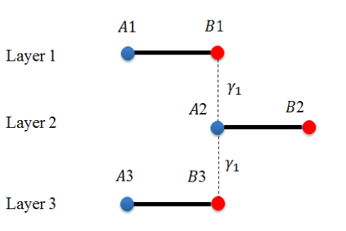
Figure 1: Crystallographic structures showing the relative position of sublattices $Ai$ and $Bi$ ($i=1,\ 2,\ 3$) for ABA-stacked trilayer graphene with intra-layer $\gamma_{1}$ hopping amplitudes.

In a basis with components of $\Psi=(\Psi_{A1},\Psi_{B1},\Psi_{A2},\Psi_{B2},\Psi_{A3},\Psi_{B3})^{T}$, the Hamiltonian of our system can be written as

$$H_{ABA}=\begin{pmatrix}u_{1}&\pi^{\dagger}&0&0&0&0\\ \pi&u_{1}&\gamma_{1}&0&0&0\\ 0&\gamma_{1}&u_{2}&\pi^{\dagger}&0&\gamma_{1}\\ 0&0&\pi&u_{2}&0&0\\ 0&0&0&0&u_{3}&\pi^{\dagger}\\ 0&0&\gamma_{1}&0&\pi&u_{3}\\ \end{pmatrix}$$ (1)

where $\Psi_{Ai}$ ($\Psi_{Bi}$) are the envelope functions associated with the probability amplitudes of the wave functions on the sublattice $A$ ($B$) of the $i^{\texttt{th}}$ layer ($i=1,2,3$), $u_{i}$ ($i=1,2,3)$ is the potential in each layer, $v_{F}=10^{6}$ m/s is the Fermi velocity. $\pi$ and $\pi^{\dagger}$ are the momentum operators in polar coordinates

$${\pi=v_{F}e^{i\theta}\left[-i\hbar\left(\frac{\partial}{\partial_{r}}+\frac{i\partial}{r\partial_{\theta}}\right)+i\frac{eB_{0}r}{2}\right]}$$ (2)

$${\pi^{\dagger}=v_{F}e^{-i\theta}\left[-i\hbar\left(\frac{\partial}{\partial_{r}}-\frac{i\partial}{r\partial_{\theta}}\right)-i\frac{eB_{0}r}{2}\right]}$$ (3)

in which the symmetric gauge is used to fix the vector potential $A=\frac{B_{0}r}{2}$.

In the next we will present analytical expression of the eigenstates and energy levels of ideal quantum ring with radius $R$ created with ABA-stacked trilayer graphene. For this system, the momentum of the charge carriers in the radial direction is zero. By freezing out the carrier radial motion, the four-component wave function becomes

$$\Psi(r,\theta)=\begin{pmatrix}\Phi_{A1}(r)e^{i(m-1)\theta}\\ i\Phi_{B1}(r)e^{im\theta}\\ i\Phi_{A2}(r)e^{im\theta}\\ \Phi_{B2}e^{i(m+1)\theta}\\ \Phi_{A3}(r)e^{i(m-1)\theta}\\ i\Phi_{B3}(r)e^{im\theta}\end{pmatrix}$$ (4)

where $m\in\mathbb{Z}$ is eigenvalues of the angular momentum label. Now solving the Dirac equation $H\Psi(R,\theta)=E\Psi(R,\theta)$ to obtain the following system of coupled differential equations

$$(u_{1}-\epsilon)\Phi_{A1}(R)+(m+\beta)\Phi_{B1}(R)=0$$ (10)

$$(m-1+\beta)\Phi_{A1}(R)+(u_{1}-\epsilon)\Phi_{B1}(R)+\gamma\Phi_{A2}(R)=0$$

$$\gamma\Phi_{B1}(R)+(u_{2}-\epsilon)\Phi_{A2}(R)-(m+1+\beta)\Phi_{B2}(R)+\gamma\Phi_{B3}(R)=0$$

$$(m+\beta)\Phi_{A2}(R)-(u_{2}-\epsilon)\Phi_{B2}(R)=0$$

$$(u_{3}-\epsilon)\Phi_{A3}(R)+(m+\beta)\Phi_{B3}(R)=0$$

$$\gamma\Phi_{A2}(R)+(m-1+\beta)\Phi_{A3}(R)+(u_{3}-\epsilon)\Phi_{B3}(R)=0$$

where we have set the dimensionless quantities $E_{0}=\frac{\hbar v_{F}}{R}$, $\gamma=\frac{\gamma_{1}}{E_{0}}$, $\epsilon=\frac{E}{E_{0}}$, $\beta=\left(\frac{eB_{0}}{2\hbar}\right)R^{2}$ and $U_{i}=\frac{u_{i}}{E_{0}}$ ($i=1,2,3$). After some straightforward algebra and fixing the potential as $u_{i}=u$, we derive the six energy band solutions

$${S_{1}^{s}=s\sqrt{(m+\beta)(m+\beta+1)}}$$ (11)

$${(S_{2}^{s})^{2}=(m+\beta)^{2}+(\gamma^{\prime})^{2}/2+s\sqrt{(m+\beta)^{2}(1+(\gamma^{\prime})^{2})+(\gamma^{\prime})^{4}/4}}$$ (12)

where $S=\epsilon-U$, $s=\pm 1$, $\gamma^{\prime}=\sqrt{2}\gamma$. We notice that (11) corresponds to energy levels of a single layer graphene, whereas (12) coincides (apart from a numerical factor $\sqrt{2}$ in front of $\gamma$) with energy levels of a bilayer graphene [33]. This is expected since the low energy band structure of ABA-staked trilayer graphene for zero magnetic field consists of two single layer graphene-like bands and four AB-staked bilayer graphene-like bands [36, 37]. From (11), we see that the energy spectrum for an ideal quantum ring, is real when $m<-\beta-1$ or $m>-\beta$ and imaginary otherwise. However for (12), the four solutions for the energy are real only when $|m+\beta|\geq 1$. In the opposite case of $|m+\beta|<1$ (or equivalently $-1+\beta<m<1-\beta$) we have $S_{2}^{-}<0$ and consequently the corresponding energies are imaginary. To solve this problem we propose the limit of $\gamma\gg m+\beta$, we obtain

$$(S_{2}^{-})^{2}=\frac{1}{(\gamma^{\prime})^{2}}(m+\beta)^{2}((m+\beta)^{2}-1)$$ (13)

and thus the energy solutions are given by

$$(S_{2}^{-})\simeq\pm\frac{1}{\gamma^{\prime}}\sqrt{(m+\beta)^{2}((m+\beta)^{2}-1)}.$$ (14)

From (11) and (12) we end up with the six band solutions

$$E_{1}^{s}=\frac{\hbar v_{F}}{R}\left[U+s\sqrt{(m+\beta)(m+\beta+1)}\right]$$ (15)

$$E_{2}^{+}=\frac{\hbar v_{F}}{R}\left[U\pm\sqrt{(m+\beta)^{2}+(\gamma^{\prime})^{2}/2+\sqrt{(m+\beta)^{2}(1+(\gamma^{\prime})^{2})+(\gamma^{\prime})^{4}/4}}\right]$$ (16)

$$E_{2}^{-}=\frac{\hbar v_{F}}{R}\left[U\pm\frac{1}{\gamma^{\prime}}\sqrt{(m+\beta)^{2}((m+\beta)^{2}-1)}\right].$$ (17)

These will numerically be analyzed based on different consideration of the involved parameters, which concern the external magnetic field and the eigenvalues of the angular momentum.

3 Results and discussions

In Figure 2, we plot the energy levels of an ideal quantum ring in ABA-stacked trilayer graphene as a function of the ring radius $R$ with $B=0$ T ((a) $u=0$ meV, (c) $u=100$ meV) and $B=5$ T ((b) $u=0$ meV, (d) $u=100$ meV). The green and red curves correspond, respectively, to $-6\leq m\leq-1$ and $1\leq m\leq 6$ while the black one correspond to $m=0$. For zero magnetic field (Figure 2(a) and (c)), we can see that the energy spectrum shows two sets of levels. One similar to the monolayer and the other corresponding to the AB-stacked bilayer graphene [33].

For a deep understanding of our results, we distinguish two cases. The first is zero magnetic field where the the energy branches take the following form

$$E_{1}^{s}=u+s\frac{\hbar v_{F}}{R}\sqrt{m(m+1)}$$ (18)

which have a $1/R$ dependence, however for large $R$, the set of levels converge to the potential $u$. Note that for $m=0$ and $m=-1$, the energy $E_{1}^{s}=u$ is independent of $R$. The second is nonzero magnetic field where the right panel (Figure 2(b) and (d)) shows that the branches have an approximately linear dependence on the ring radius for large $R$. This is

$$E_{1}^{s}=u+s\frac{v_{F}eB}{2}R.$$ (19)

However, for small $R$, all branches diverge as $1/R$ except for two values $m=0$ and $m=-1$, which give the result

$$E_{1}^{s}=u+s\frac{\hbar}{R}\sqrt{m(m+1)}$$ (20)

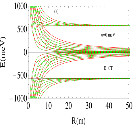
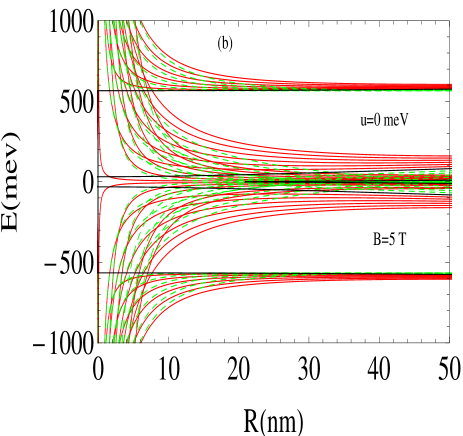
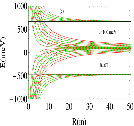
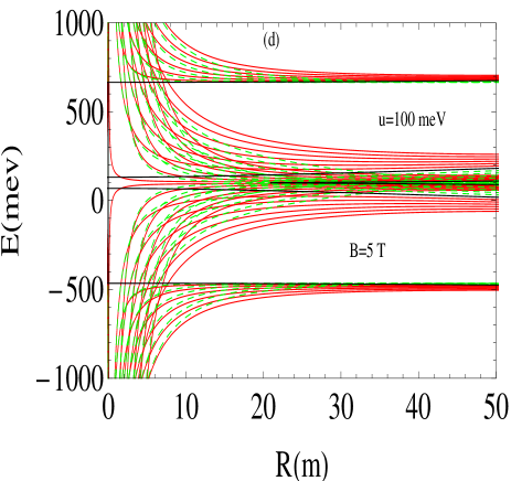
Figure 2: Energy levels of a trilayer graphene quantum ring as function of ring radius $R$ with $B=0$ T ((a): $u=0$ meV and (c): $u=100$ meV) and $B=5$ T ((b): $u=0$ meV and (d): $u=100$ meV). The total angular quantum number $-6\leq m\leq-1$ (green), $1\leq m\leq 6$ (red) and $m=0$ (black).

and in addition, for zero magnetic field and for large radius the energy branches approach as $E\longrightarrow\pm\sqrt{2}\gamma$. We notice that from (12) and for zero magnetic field, we have the energy branches

$$E_{2}^{+}=u\pm\sqrt{\frac{(\hbar v_{F})^{2}}{R^{2}}m^{2}+\gamma_{1}^{2}+\sqrt{\gamma_{1}^{4}+\left(m^{2}\frac{(\hbar v_{F})^{4}}{R^{4}}+2\gamma_{1}^{2}\frac{(\hbar v_{F})^{2}}{R^{2}}\right)}}$$ (21)

$$E_{2}^{-}=u\pm\frac{(\hbar v_{F})^{2}}{\sqrt{2}\gamma_{1}R^{2}}\sqrt{m^{2}(m^{2}+1)}.$$ (22)

From these results, one can deduce different conclusions. Indeed, Firstly, we can clearly show that, for zero magnetic field, the second set of energy levels depends on $1/R^{2}$. Secondly, in the limit $R\longrightarrow\infty$, we have $E^{-}_{2}\longrightarrow u$ and $E^{+}_{2}\longrightarrow u+\sqrt{2}\gamma_{1}$. Thirdly when $R\longrightarrow 0$, the behavior of the spectrum is different and the corresponding energy levels diverge. In addition, we note that the applied potential has different effect on the system behavior compared to that in the case of AB-stacked bilayer quantum ring [33]. Indeed, in our system when $u=100$ meV all sets are shifted up by $u$, however in the case of ideal quantum rings in AB-stacked bilayer the application of the potential open a gap in the energy spectrum.

Now we return back to investigate the basic features of (16) and (17). Indeed, in the case of non zero magnetic field and for small ring radius $R$, both equations reduce

$$E_{2}^{+}=u\pm\frac{\hbar v_{F}}{R}\sqrt{m^{2}+\mid m\mid}$$ (23)

$$E_{2}^{-}=u\pm\frac{(\hbar v_{F})^{2}}{\sqrt{2}\gamma_{1}R^{2}}\sqrt{m^{2}(m^{2}+1)}$$ (24)

depending on $1/R$ and $1/R^{2}$, respectively. However for large radius $R$, (16) and (17) give the results

$$E_{2}^{+}=u\pm\frac{(v_{F}eB/2)^{2}}{\sqrt{2}\gamma_{1}}R^{2}$$ (25)

$$E_{2}^{-}=u\pm\frac{eBv^{2}_{F}}{2}R.$$ (26)

which explain the approximately $R^{2}$ dependence of the energy branches on the radius of the ring and also the approximately linear dependence of the energy branches on the ring radius. It is important to note that, for zero magnetic field, all branches are twofold degenerate. However, the application of a nonzero magnetic field breaks the degeneracy of all branches.

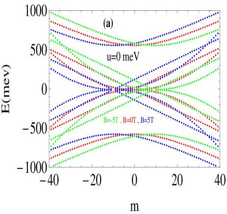
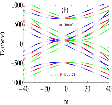
Figure 3: Energy levels of a trilayer graphene quantum ring as as function of total angular momentum label $m$ for $B=-5$ T (geen), $B=0$ T (reed) and $B=5$ T (blue) and $R=50$ nm. (a): $u=0$ meV, (b): $u=100$ meV.

In Figure 3, we plot the energy levels of an ideal quantum ring of ABA-stacked trilayer graphene as a function of the angular momentum $m$ for three different values of the magnetic field ($B=-5$ T) (green), $B=0$ T (red) and $B=5$ T (blue) for $R=50$ nm with $u=0$ meV (Figure 3(a)) and $u=100$ meV (Figure 3(b)). The energy spectrum represents two bands dispersed with an energy (11), which is quite similar to that of an single layer (linear dispersion), and four bands of type bilayer graphene (parabolic dispersion) (14) and (15). We notice that, like the case of monolayer [33] and AB-stacked bilayer graphene [38], the electron energy present a minimum for a particular value of the angular momentum $m$. The energy minimum for $B=-5$ T is given by $m=10$. However, the energy minimum for $B=0$ T and $B=5$ T, are respectively, given by $m=0$ and $m=10$. This can be explained by the fact that from (15)-(17), the spectra are invariant under the transformation $B\longrightarrow-B$, $m\longrightarrow-m$ and $m\longrightarrow-(m+1)$. Therefore, the energies satisfy the following symmetries with respect to the above transformations

$$E_{1}^{s}(m,B)=E_{1}^{s}(-m-1,-B)$$ (27)

$$E_{2}^{+}(m,B)=E_{2}^{+}(-m,-B)$$ (28)

$$E_{2}^{-}(m,B)=E_{2}^{-}(-m,-B).$$ (29)

These symmetries are also present in the case of ideal quantum ring in monolayer and bilayer graphene systems [33].

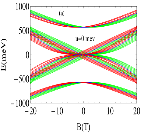
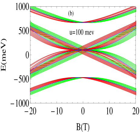
Figure 4: Electron and hole energy states of a trilayer graphene quantum ring as as function of external magnetic field $B$ for $R=50$ nm. $-6\leq m\leq-1$ (green curves), $1\leq m\leq 6$ (red curves) and $m=0$ (blue curves).

The energy levels of the electrons and holes for an ideal quantum ring in a ABA-stacked trilayer graphene as function of the external magnetic field are shown in Figure 4 for $R=50$ nm, with (a): $u=0$ meV, (b): $u=100$ meV. The energy levels are show for the quantum number $-6\leq m\leq-1$ (green), $1\leq m\leq 6$ (red) and $m=0$ (blue). We can clearly show, for $u=0$ meV (Figure 4(a)), that the energy spectrum presents two sets of energy levels, one is similar to the energy levels of AB-stacked bilayer graphene quantum ring that are parabolically disperses with $B$, and the second one correspond to the monolayer graphene quantum ring that are dispersing linearly with $B$. Note that when $u\neq 0$, the energy levels are shifted vertically by $u$ (Figure 4(b)). This results are not similar to that obtained for AA-stacked [34] and AB-stacked [33] bilayer graphene quantum ring, where the application of a potential $\neq 0$ open a gap in the energy spectrum. From Figure 4(b), we can show that there is an asymmetry between the electron and hole states caused by the application of the potential. Also, these results show that the electron and hole energies are related by

$$E_{1(e)}^{s}(m,B)=-E_{1(h)}^{s}(-m-1,-B)$$ (30)

$$E_{2(e)}^{+}(m,B)=-E_{2(h)}^{+}(-m,-B)$$ (31)

$$E_{2(e)}^{-}(m,B)=-E_{2(h)}^{-}(-m,-B)$$ (32)

where the indices $h(e)$ refer to holes (electrons). These results are similar to that obtained for a finite width quantum ring in monolayer graphene and AB-stacked bilayer graphene [33].

4 Conclusion

In summary, we have investigated the behavior of charge carriers in ideal quantum rings of ABA-stacked subjected to a perpendicular magnetic field. The calculation was performed by solving the Dirac equation for a zero width ring geometry (ideal ring). In the case of an ideal ring with radius $R$, the momentum of the carriers in the radial direction is zero, then we have to treat the radial parts of the spinors as a constant. Our approach lead to analytical expressions of the energy spectrum as a function of the ring radius and the magnetic field.

Our results show that the energy spectrum of an ideal quantum ring presents two sets of states as a function of the ring radius $R$. One corresponding to the monolayer graphene and the other corresponding to the AB-stacked bilayer graphene quantum ring. We have shown that, for large $R$, the set of energy levels that correspond to the monolayer graphene converge to $\sqrt{2}\gamma$. The energy branches corresponding to the monolayer graphene have a $1/R$ dependence, whereas the energy branches corresponding to the bilayer graphene have a dependence $1/R^{2}$. This implied that the energy spectrum converge to $u$ and $u+\sqrt{2}\gamma$ for a very large radius and diverges when the radius tends to zero. In the absence of the magnetic field, the energy levels are twofold degenerate. The application of nonzero magnetic field broken all the degeneracy of all branches and the obtained spectrum exhibited different symmetries. In addition, our numerical results showed that the electron and hole energy levels are not invariant under the transformation $B\longrightarrow-B$, $m\longrightarrow-m$ and $m\longrightarrow-(m+1)$. The application of a potential lead to a vertically shifting of the energy spectrum. These results are not similar to those obtained for AA-stacked and AB-stacked bilayer quantum ring, where the application of a potential open a gap in the energy spectrum.

References

- [1] A. K. Geim, and K. S. Novoselov, Nat. Mat. 6, 183 (2007).
- [2] F. Guinea, M. I. Katsnelson, and A. K. Geim, Nat. Phys. 6, 30 (2009).
- [3] A. H. Castro Neto, F. Guinea, N. M. R. Peres, K. S. Novoselov, and A. K. Geim, Rev. Mod. Phys. 81, 109 (2009).
- [4] A. D. Martino, A. Hutten, and R. Egger, Phys. Rev. B 84, 155420 (2011).
- [5] K. S. Novoselov, A. K. Geim, S. V. Morozov, D. Jiang, M. I. Katsnelson, I. V. Grigorieva, S. V. Dubonos, and A. A. Firsov, Nature 438, 197 (2005).
- [6] Y. Zhang, Y. W. Tan, H. L. Stormer, and P. Kim, Nature 438, 201 (2005).
- [7] M. I. Katsnelson, K. S. Novoselov, and A. K. Geim, Nat. Phys. 2, 620 (2006).
- [8] G. W. Semenoff, Phys. Rev. Lett. 53, 2449 (1984).
- [9] D. P. DiVincenzo, and E. J. Mele, Phys. Rev. B 29, 1685 (1984).
- [10] A. Avetisyan, B. Partoens, and F. M. Peeters, Phys. Rev. B 81, 115432 (2010).
- [11] M. F. Craciun, S. Russo, M. Yamamoto, J. B. Oostinga, A. F. Morpurgo, and S. Tarucha, Nat. Nanotechnol. 4, 383 (2009).
- [12] J. H. Warner, Nanotechnology 21, 255707 (2010).
- [13] K. F. Mak, J. Shan, and T. F. Heinz, Phys. Rev. Lett. 104, 176404 (2010).
- [14] F. Zhang, B. Sahu, H. Min, and A. H. MacDonald, Phys. Rev. B 82, 035409 (2010).
- [15] E. McCann, and M. Koshino, Phys. Rev. B 81, 241409 (2010).
- [16] C. L. Lu, C. P. Chang, Y. C. Huang, R. B. Chen, and M. L. Lin, Phys. Rev. B 73, 144427 (2006).
- [17] F. Guinea, A. H. Castro Neto, and N. M. R. Peres, Phys. Rev. B 73, 245426 (2006).
- [18] S. Latil, and L. Henrard, Phys. Rev. Lett. 97, 036803 (2006).
- [19] B. Partoens and F. M. Peeters, Phys. Rev. B 74, 075404 (2006).
- [20] M. Koshino, and T. Ando, Phys. Rev. B 76, 085425 (2007).
- [21] M. Aoki, and H. Amawashi, Solid State Commun. 142, 123 (2007).
- [22] S. Russo, J. B. Oostinga, D. Wehenkel, H. B. Heersche, S. S. Sobhani, L. M. K. Vandersypen, and A. F. Morpurgo, Phys. Rev. B 77, 085413 (2008).
- [23] K. S. Novoselov, Z. Jiang, Y. Zhang, S. V. Morozov, H. L. Stormer, U. Zeitler, J. C. Maan, G. S. Boebinger, P. Kim, and A. K. Geim, Science 315, 1379 (2007).
- [24] L. A. Ponomarenko, F. Schedin, M. I. Katsnelson, R. Yang, E. W. Hill, K. S. Novolevov, and A. K. Geim, Science 320, 356 (2008).
- [25] T. Schen, Y. Q. Wu, M. A. Capano, L. P. Robickinson, L. W. Engel, and P. D. Ye, Appl. Phys. Lett. 93, 122102 (2008).
- [26] T. Yamamoto, T. Noguchi, and K. Watanabe, Phys. Rev. B 74, 121409 (2006).
- [27] Z. Z. Zhang, K. Chang, and F. M. Peeters, Phys. Rev. B 77, 235411 (2008).
- [28] P. Recher, B. Trauzettel, A. Rycerz, C. W. J. Beenakker, and A. F. Morpurgo, Phys. Rev. B 76, 235404 (2007).
- [29] D. S. L. Abergel, V. M. Apalkov, and T. Chakraborty, Phys. Rev. B 78, 193405 (2008).
- [30] T. G. Pedersen, C. Flindt, J. Pedersen, N. A. Mortensen, A. P. Jauho, and K. Pedersen, Phys. Rev. Lett. 100, 136804 (2008).
- [31] T. G. Pedersen, C. Flindt, J. Pedersen, A. P. Jauho, N. A. Mortensen, and K. Pedersen, Phys. Rev. B 77, 245431 (2008).
- [32] M. Huefner, F. Molitor, A. Jacobsen, A. Pioda, C. Stampfer, K. Ensslin, and T. Ihn, New J. Phys. 12, 043054 (2010).
- [33] M. Zarenia, J. M. Pereira, A. Chaves, F. M. Peeters, and G. A. Farias, Phys. Rev. B 81, 045431 (2010).
- [34] Y. Zahidi, A. Belouad, and Ahmed Jellal, Mater. Res. Express 4, 055603 (2017).
- [35] M. S. Dresselhaus, and G. Dresselhaus, Adv. Phys. 51, 1 (2002).
- [36] S. Yuan, R. Roldan, and M. I. Katsnelson, Phys. Rev. B 84, 125455 (2011).
- [37] B. Van Duppen, S. H. R. Sena, and F. M. Peeters, Phys. Rev. B 87, 195439 (2013).
- [38] D. R. da Costa, M. Zarenia, A. Chaves, G. A. Farias, and F. M. Peeters, Carbon 78, 392400 (2014).