Transition of EMRIs through resonance: corrections to higher order in the on-resonance flux modification

Deyan P. Mihaylov d.mihaylov@ast.cam.ac.uk Institute of Astronomy, University of Cambridge, Madingley Road, Cambridge, CB3 0HA    Jonathan R. Gair j.gair@ed.ac.uk Institute of Astronomy, University of Cambridge, Madingley Road, Cambridge, CB3 0HA School of Mathematics, University of Edinburgh, Peter Guthrie Tait Road, Edinburgh, EH9 3FD
Abstract

Extreme-mass-ratio inspirals (emris) are candidate events for gravitational wave detection in the millihertz band (by detectors like lisa). These events involve a stellar-mass black hole, or a similar compact object, descending in the gravitational field of a supermassive black hole, eventually merging with it. Properties of the inspiralling trajectory away from resonance are well known and have been studied extensively, however little is known about the behaviour of these binary systems at resonance, when the radial and lateral frequencies of the orbit become commensurate. We describe the two existing models, the instantaneous frequency approach used by Gair, Bender, and Yunes, and the standard two timescales approach implemented by Flanagan and Hinderer. In both cases, the exact treatment depends on the modelling of the gravitational self-force, which is currently not available. We extend the results in Gair, Bender and Yunes to higher order in the on-resonance flux modification, and argue that the instantaneous frequency approach is also a valid treatment of the resonance problem. The non-linear differential equations which arise in treating resonances are interesting from a mathematical view point. We present our algorithm for perturbative solutions and the results to third order in the infinitesimal parameter, and discuss the scope of this approach.

I Introduction

Gravitational waves are one of the most fascinating predictions of general relativity. The theoretical underpinning for them was first presented by Einstein (1918). In 1974, Taylor and Hulse discovered indirect evidence for their existence when they observed the first pulsar in a binary system, in which the object separation was gradually decreasing, and were the first to suggest that gravitational wave effects are at play (Hulse and Taylor, 1975; Taylor and Weisberg, 1982). The pair were awarded the Nobel Prize in Physics in 1993 for their discovery – until recently the only evidence for the existence of gravitational waves. Nearly a century after Einstein’s paper, gravitational waves were directly observed for the first time in September 2015 by the two advanced ligo detectors, thus culminating a decades-long efforts to detect gravitational radiation (Abbott et al., 2016a). Currently, several experiments, including Advanced ligo and Advanced Virgo, which are searching for waves in the range 102 Hz - 104 HzrangetimesE2hertztimesE4hertz{10}^{2}\text{\,}\mathrm{Hz}{10}^{4}\text{\,}\mathrm{Hz} (The LIGO Scientific Collaboration et al., 2015; Acernese et al., 2015), are being deployed to search for further signals. The first joint run is scheduled to take place in late 2016 or early 2017 (Abbott et al., 2016b) and it is expected that a significant number of events will be observed in the near future (Abadie et al., 2010; The LIGO Scientific Collaboration et al., 2016). The European Space Agency has selected gravitational wave detection from space as the science theme to be addressed by the L3 large satellite mission, currently scheduled for launch in 2034. This space-based detector, called Laser Interferometer Space Antenna (lisa), will operate in the millihertz frequency range. The mission design is still being formulated, but it will be finalised by the end of this decade (Amaro-Seoane et al., 2012). The need for multiple approaches to detection (currently there are more than a dozen projects, both ground- and space-based, see Moore et al. (2015) for an overview) is driven by the broad spectrum of gravitational wave frequencies (the typical frequency of a gravitational wave system is given by f(GM/L3)1/2similar-to𝑓superscript𝐺𝑀superscript𝐿312f\sim(GM/L^{3})^{1/2}, where M𝑀M is the mass of the system, and L𝐿L is its length scale), namely in the range 1016 Hz - 104 HzrangetimesE-16hertztimesE4hertz{10}^{-16}\text{\,}\mathrm{Hz}{10}^{4}\text{\,}\mathrm{Hz}, produced by a variety of potential gravitational radiation sources (Thorne, 1995).

Systems which are expected to produce gravitational waves are those that are accelerating and exhibit asymmetry in their configuration: for instance a binary (Aasi et al., 2014), a supernova (Gossan et al., 2016), or a spinning star with a pronounced bulge. Among the range of binary celestial systems, we focus on the case of a compact object (of several solar masses, usually a stellar-mass black hole, or a neutron star) gradually spiralling towards a supermassive black hole (typically between 105superscript10510^{5} and 1012superscript101210^{12} solar masses, although the ones of interest to us are between 105superscript10510^{5} and 107superscript10710^{7} Msubscript𝑀direct-productM_{\odot}, since these generate gravitational waves at frequencies in the range of sensitivity of lisa (Amaro-Seoane et al., 2012; Babak et al., 2015)). Since the mass m𝑚m of the compact object is in the range of 10102M10superscript102subscript𝑀direct-product10-10^{2}M_{\odot}, the ratio of the masses is typically ϵ=m/M106 to 104italic-ϵ𝑚𝑀similar-tosuperscript106 to superscript104\epsilon=m/M\sim 10^{-6}\text{ to }10^{-4}. Termed extreme-mass-ratio inspirals (emris), these binaries are expected to radiate gravitational waves with frequency in the range 104 Hz - 102 HzrangetimesE-4hertztimesE-2hertz{10}^{-4}\text{\,}\mathrm{Hz}{10}^{-2}\text{\,}\mathrm{Hz}. This fact places them in a position to be likely candidates for detection by the lisa mission. emris reside near the centres of galaxies (where supermassive black holes are situated (Kormendy and Richstone, 1995)) and clusters of stars and stellar remnants are available for capture by the black hole. Plenty of scientific effort has been invested into modelling the evolution of emris (Barack and Cutler, 2004; Gair and Glampedakis, 2006; Drasco and Hughes, 2006; Chua and Gair, 2015), computing their waveforms (Babak et al., 2007), predicting the rates and timescales of inspiral (Glampedakis et al., 2002; Hopman, 2009), and estimating the parameters of the orbit (Barack and Cutler, 2004; Arun et al., 2009). Applications of gravitational wave observations of emris to inference on astrophysical populations (Gair et al., 2010), cosmology (MacLeod and Hogan, 2008) and fundamental physics (Gair et al., 2013) have also been explored in detail.

The mass of the compact object in an emri is typically at least 4 orders of magnitude smaller than the mass of the supermassive black hole. This allows us to treat the presence of the compact body in the background space-time of the central object as a perturbation. According to the uniqueness theorem for black holes, they can be uniquely characterised by three parameters - mass, spin and charge. Since electromagnetic repulsion is much stronger than gravitational attraction (about 40 orders of magnitude), we can assume that astrophysical black holes have negligible net charge. Hence, we consider the Kerr metric, where black holes are described only by their mass and spin. The Kerr space-time is well-known, with a complete set of integrals of motion, and the geodesics can be characterised by three constants (Carter (1968) and Appendix B). For a point mass, the trajectory would be that of a geodesic around the black hole, but while the point-mass notion is convenient mathematically, it does not apply in the context of the current problem. Therefore, we need to address the finite size and mass of the compact object. The deviation from geodesic motion can be quantified by allowing for the gravitational self-force on the compact object, (Nakamura and Sasaki, 1982; Wardell et al., 2012), also known as the gravitational radiation reaction force, since it is responsible for the gravitational radiation emission from the object. There is a radiative component of the self-force that leads to evolution of the orbital frequencies, as well as a conservative component that changes the instantaneous values of the orbital frequencies. The trajectory can be modelled as a sequence of geodesics, each one with lower energy than the previous one, and therefore (on average) closer to the central object. This method is called the osculating element approach (Pound and Poisson, 2008; Gair et al., 2011; Sopuerta and Yunes, 2012). Individual orbits are well approximated as geodesics, however the defining parameters of these geodesics are continuously changing, and this is what shapes the inspiral orbit. This effect will be visible over a large number of orbits – typically over a timescale of 𝒪(ϵ1)𝒪superscriptitalic-ϵ1\mathcal{O}\!\left(\epsilon^{-1}\right).

As the test body progresses along its in-spiral, at certain points two of the three frequencies of motion will become rational multiples of each other, putting the system into resonance (Flanagan and Hinderer, 2012). While in general the behaviour of the inspiral is well-studied and modelled (Barack, 2009), during resonance the system exhibits unusual behaviour, accompanied by changes in the orbital parameters (Flanagan and Hinderer, 2012). The evolution of emris during resonances, and their effect on gravitational wave emission is currently an interesting topic in gravitational wave astronomy (Berry et al., 2016).

There are two approaches in the literature that treat the behaviour of extreme-mass-ratio inspirals on resonance. On one hand is the instantaneous value treatment by (Gair et al., 2010), with manifestations in both frequency and phase formalisms, and on the other is the approach by (Flanagan and Hinderer, 2012), which separates the timescales associated with the in-spiral into small and large. We will describe both methods here, but focus on extending the former approach to higher order, as we anticipate the predictions of the latter to be consistent with the phase formalism in the former.

I.1 The Gravitational Self-force

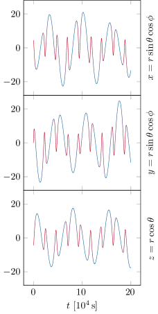
The geodesic principle of General Relativity dictates that free point particles, of zero mass, traverse time-like geodesics of the space-time. Unfortunately, while treating bodies in General Relativity as point masses is mathematically convenient, in reality this approach is far from accurate, and introduces immense difficulties to the problem we are considering. As the size R𝑅R of a body is scaled down to 0, its mass M𝑀M should decrease accordingly, scaling to 0 at the same time as the size of the body (Gralla and Wald, 2008), otherwise a black hole solution would form before the point-limit of the body is reached. We can account for the finite size and mass of the body if we consider the effect of these on the deviation from geodesic motion. At leading order, we ignore the presence of the space-time generated by the compact object in the background space-time, and in this idealised system, the test body follows a time-like geodesic, whose shape can be accurately computed (see Appendix C and Figure C for details). The next order accounts for the non-infinitesimal size and mass of the object, and this causes a deviation from the geodesic motion described above. We quantify this phenomenon by introducing the gravitational self-force, responsible for the inward spiral of the compact object (Nakamura and Sasaki, 1982; Flanagan and Hinderer, 2012). This force is at the same time responsible for dissipating the energy made available by the inspiral motion in the form of gravitational radiation.

A proper treatment of the gravitational self-force is not the objective of this paper. The reader may wish to consult Poisson et al. (2011), as well as the more concise review Poisson (2011). Further recommended reading is Nakamura and Sasaki (1982) and Wald (2011), or the more mathematical approach described in Gralla and Wald (2008).

In the context of this article, it is worth knowing that since the self-force is the perturbation in the mass parameter to the geodesic, its leading order dependence on the mass of the test body is linear. Further, the self-force will depend on the shape of the orbit, which for the Kerr space-time is specified by three constants of the motion, for example the energy \mathcal{E}, the 3rd component of the angular momentum zsubscript𝑧\mathcal{L}_{z}, and Carter’s constant, 𝒬𝒬\mathcal{Q}. Furthermore, the individual components of this self-force will depend on the position of the test body along the orbit, specified, for example, by the action-angle coordinates qαsubscript𝑞𝛼q_{\alpha}, where the index α{t,r,θ,ϕ}𝛼𝑡𝑟𝜃italic-ϕ\alpha\in\{t,r,\theta,\phi\} (this implies there are 4 separate action-angle coordinates, with 4 corresponding components of the self-force. In fact, only 3 of these force components are independent, as can be verified by differentiating the condition gαβuαuβ=1subscript𝑔𝛼𝛽superscript𝑢𝛼superscript𝑢𝛽1g_{\alpha\beta}u^{\alpha}u^{\beta}=1 with respect to the proper time τ𝜏\tau to obtain uαaα=0superscript𝑢𝛼subscript𝑎𝛼0u^{\alpha}a_{\alpha}=0 (Gair et al., 2011)). With this in mind, we can assume that the linear order gravitational self-force can be written in the form (Poisson, 2011; Gair, Yunes, and Bender, 2012)

aα=d2xαdτ2=ϵFα(𝐪,𝐉),subscript𝑎𝛼superscriptd2subscript𝑥𝛼dsuperscript𝜏2italic-ϵsubscript𝐹𝛼𝐪𝐉\displaystyle a_{\alpha}=\frac{\mathop{}\!\mathrm{d}^{2}x_{\alpha}}{\mathop{}\!\mathrm{d}\tau^{2}}=\epsilon\,F_{\alpha}(\mathbf{q},\mathbf{J}), (1)

where ϵ=m/Mitalic-ϵ𝑚𝑀\epsilon=m/M is the ratio of the compact object mass to the mass of the supermassive black hole, and the vector 𝐉𝐉\mathbf{J} contains the three constants of motion defining the shape of the orbit. The values of 𝐪𝐪\mathbf{q} and 𝐉𝐉\mathbf{J} in general depend on the way the orbit evolved before the moment at which they are computed. Thus, it can be regarded that the instantaneous self-force is in fact given by an integral over the past history of the orbit.

I.2 Orbital resonances

We already reasoned why the gravitational self-force depends on the shape of the orbit, i.e. the values of the three constants of motion in the Kerr metric. These quantities can be mapped to the three fundamental frequencies of orbital motion {ωr,ωθ,ωϕ}subscript𝜔𝑟subscript𝜔𝜃subscript𝜔italic-ϕ\{\omega_{r},\omega_{\theta},\omega_{\phi}\} (Schmidt, 2002). Therefore, instead of eq. (1), we can write the expression for the self-force as ϵ𝐅(𝐪,𝝎)italic-ϵ𝐅𝐪𝝎\epsilon\,\mathbf{F}(\mathbf{q},\bm{\omega}). The fundamental frequencies are another valid way to label orbits of the Kerr space-time, and can be used in lieu of the geodesic constants of motion. It should be noted that the reverse substitution, from 𝝎𝝎\bm{\omega} to 𝐉𝐉\mathbf{J} is not always possible, on the account of the isofrequency pairs exhibited by the proper time frequencies (Warburton et al., 2013). For the discussion in this paper, we can assume local invertibility, however it should be noted that this is not universal.

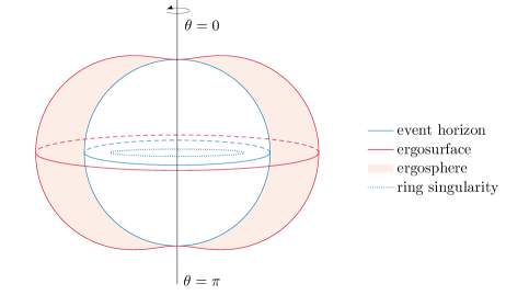
The three fundamental frequencies evolve independently according to their equations of motion. However, at certain points along the trajectory, two of the frequencies will become commensurate, and the system will temporarily exhibit a qualitatively different behaviour, a resonance, with a reduced number of degrees of freedom. Since the Kerr metric (Appendix A and Figure 23) does not depend explicitly on the azimuthal angle ϕitalic-ϕ\phi, the corresponding fundamental frequency ωϕsubscript𝜔italic-ϕ\omega_{\phi} is not relevant for any resonant motion. While the azimuthal frequency is trivial, the radial and the polar frequencies will have independently varying values along the in-spiral. Resonance occurs when these two frequencies become commensurate with each other, or, in more formal terms, when their ratio is a rational number (Ruangsri and Hughes, 2014):

ωrωθ=nθnr,{nr,nθ}.formulae-sequencesubscript𝜔𝑟subscript𝜔𝜃subscript𝑛𝜃subscript𝑛𝑟subscript𝑛𝑟subscript𝑛𝜃\displaystyle\frac{\omega_{r}}{\omega_{\theta}}=\frac{n_{\theta}}{n_{r}},\quad\{n_{r},n_{\theta}\}\subset\mathbb{Z}. (2)

During resonance, the apparent effect of the self-force on the orbit is modified, in particular there is a fractional change of order 𝒪(ϵ0)𝒪superscriptitalic-ϵ0\mathcal{O}\!\left(\epsilon^{0}\right) to the dynamics of the in-spiral – the evolution rate of parameters and the in-spiral rate (Flanagan and Hinderer, 2012). A typical emri passes through several resonance points before the two objects merge. Obviously, this complicates the numerical analysis of the in-spiral, since one has to develop a formalism to account for the occurrence of resonances, and to quantify the effects these have on the orbital dynamics (Flanagan and Hinderer, 2012).

In the current paper, we will first describe the two approaches to resonance modelling that have appeared in the literature, which were suggested by (Hinderer and Flanagan, 2008) and (Gair, Yunes, and Bender, 2012). We then describe what the differences in the model assumptions are, explain why there is a preferred case of physical relevance to resonances in emris, and argue that full knowledge of the self-force is required to robustly identify the most relevant model. We will then extend the results of (Gair, Yunes, and Bender, 2012) to obtain complete results describing the transition through resonance in that model, at leading order in the mass-ratio.

II Instantaneous frequency approach

This method is described in detail in Gair, Yunes, and Bender (2012), although here we will give an outline of the approach to aid further discussions. As explained above, individual orbits of the compact object around the black hole can be thought of as tri-periodic geodesics with fundamental frequencies {ωr,ωθ,ωϕ}subscript𝜔𝑟subscript𝜔𝜃subscript𝜔italic-ϕ\{\omega_{r},\omega_{\theta},\omega_{\phi}\}. This encourages us to employ the “osculating element” formalism, where the in-spiral is modelled as a sequence of geodesics, with the constants of motion continuously evolving as the orbit approaches the black hole, and furthermore, the effect of the compact body on the trajectory can be treated as a perturbation (Pound and Poisson, 2008). Since these constants of the motion do not change on a given geodesic, at leading order, and only evolve (continuously) as the object spirals into the supermassive black hole, we can argue that, to leading order, this effect is driven by the self-force on the object. Hence, we can write the evolution equation for Jμ=(,z,𝒬)subscript𝐽𝜇subscript𝑧𝒬J_{\mu}=(\mathcal{E},\mathcal{L}_{z},\mathcal{Q}) as follows:

dJμdτ=ϵμ(𝐪,𝐉,𝐅)+𝒪(ϵ2),dsubscript𝐽𝜇d𝜏italic-ϵsubscript𝜇𝐪𝐉𝐅𝒪superscriptitalic-ϵ2\displaystyle\frac{\mathop{}\!\mathrm{d}J_{\mu}}{\mathop{}\!\mathrm{d}\tau}=\epsilon\,\mathcal{F}_{\mu}(\mathbf{q},\mathbf{J},\mathbf{F})+\mathcal{O}\!\left(\epsilon^{2}\right), (3)

where μsubscript𝜇\mathcal{F}_{\mu} is a function of the coordinates, the generalised coordinates, and the self-force, which describes the rate of change of orbital parameters as the object moves along the inspiral. We argued that the self-force is itself a function of the coordinates and the fundamental frequencies (see Section I.2), hence we can write μ=μ(𝐪,𝝎)subscript𝜇subscript𝜇𝐪𝝎\mathcal{F}_{\mu}=\mathcal{F}_{\mu}(\mathbf{q},\bm{\omega}). Similarly, the action-angle coordinates of the system evolve proportionally to the fundamental frequencies, with a correction owing to the self-force:

dqμdτ=ωμ+ϵμ(𝐪,𝝎)+𝒪(ϵ2).dsubscript𝑞𝜇d𝜏subscript𝜔𝜇italic-ϵsubscript𝜇𝐪𝝎𝒪superscriptitalic-ϵ2\displaystyle\frac{\mathop{}\!\mathrm{d}q_{\mu}}{\mathop{}\!\mathrm{d}\tau}=\omega_{\mu}+\epsilon\,\mathcal{H}_{\mu}(\mathbf{q},\bm{\omega})+\mathcal{O}\!\left(\epsilon^{2}\right). (4)

We will not concern ourselves with the precise form of the functions μsubscript𝜇\mathcal{F}_{\mu} and μsubscript𝜇\mathcal{H}_{\mu}, but rather will point out that they can be expanded in tri-harmonic Fourier series as discussed above, which is valid without any loss of generality. ωμsubscript𝜔𝜇\omega_{\mu} is the instantaneous value of the frequency at this moment along the trajectory. This is calculated according to eq. (3), and the value is continuously updated to reflect the motion of the body along its inspiral and the effect of the self-force. Without the self-force, the frequencies will, of course, remain constant, since the trajectory would be that of a geodesic around the black hole, unaffected by gravitational wave emission.

Before carrying out the Fourier mode expansion, we recall that a geodesic in Kerr space-time is uniquely specified by three constants. Instead of the orbital parameters \mathcal{E}, zsubscript𝑧\mathcal{L}_{z}, and 𝒬𝒬\mathcal{Q}, we could use the set of fundamental frequencies – the radial frequency, ωrsubscript𝜔𝑟\omega_{r}, the polar frequency, ωθsubscript𝜔𝜃\omega_{\theta}, and the azimuthal frequency, ωϕsubscript𝜔italic-ϕ\omega_{\phi}, to specify the geodesics, as these are constant along a given geodesic. Since these can be mapped to the aforementioned integrals of the motion (Schmidt, 2002), we can use these maps to argue that the fundamental frequencies evolve along the trajectory according to a differential equation of the same form as eq. (3):

dωμdτ=ϵ𝒢μ(𝐪,𝝎)+𝒪(ϵ2).dsubscript𝜔𝜇d𝜏italic-ϵsubscript𝒢𝜇𝐪𝝎𝒪superscriptitalic-ϵ2\displaystyle\frac{\mathop{}\!\mathrm{d}\omega_{\mu}}{\mathop{}\!\mathrm{d}\tau}=\epsilon\,\mathcal{G}_{\mu}(\mathbf{q},\bm{\omega})+\mathcal{O}\!\left(\epsilon^{2}\right). (5)

The two orbital frequencies relevant to the occurrence of resonances are the radial and the polar (lateral) frequencies. As noted previously, the third frequency ωϕsubscript𝜔italic-ϕ\omega_{\phi}, that of azimuthal motion, does not play a role in the occurrence of resonances due to the axisymmetric nature of the Kerr space-time. We use this property to write a bi-periodic expansion for the function of the self-force in Fourier modes of the two frequencies {ωr,ωθ}subscript𝜔𝑟subscript𝜔𝜃\{\omega_{r},\omega_{\theta}\}:

dωμdτ=ϵl,m(Almcos[(lωr+mωθ)τ]+Blmsin[(lωr+mωθ)τ])+𝒪(ϵ2).dsubscript𝜔𝜇d𝜏italic-ϵsubscript𝑙𝑚subscript𝐴𝑙𝑚𝑙subscript𝜔𝑟𝑚subscript𝜔𝜃𝜏subscript𝐵𝑙𝑚𝑙subscript𝜔𝑟𝑚subscript𝜔𝜃𝜏𝒪superscriptitalic-ϵ2\displaystyle\begin{split}\frac{\mathop{}\!\mathrm{d}\omega_{\mu}}{\mathop{}\!\mathrm{d}\tau}=\epsilon\sum_{l,\,m}&\left(A_{lm}\cos\!\Big{[}\!\left(l\omega_{r}+m\omega_{\theta}\right)\tau\Big{]}\vphantom{\Big{[}\Big{]}^{\!\!\!2\,}}\right.\\ &\left.\vphantom{\Big{[}\Big{]}^{\!\!\!2\,}}\!\!\!+B_{lm}\sin\!\Big{[}\!\left(l\omega_{r}+m\omega_{\theta}\right)\tau\Big{]}\right)\!+\mathcal{O}\!\left(\epsilon^{2}\right).\end{split} (6)

We can regard this equation as an adiabatic evolution equation – at leading order the terms on the right-hand side are constant in time since they are taken along the same geodesic, while the differential on the left-hand side expresses their evolution along the trajectory of the compact object towards the black hole. Of course, the quantities on the right-hand side are instantaneous, and their values are constantly updated through the evolution equations. The sum is over the non-negative integers l𝑙l and m𝑚m. Since we have written the time-dependence explicitly in the Fourier series, the coefficients of the expansion depend smoothly on the constant parameters of the geodesic. Therefore, we can expand the coefficients in orders of the mass ratio, and neglect all terms sub-leading in ϵitalic-ϵ\epsilon.

Alternatively, instead of using the {ωμ}subscript𝜔𝜇\{\omega_{\mu}\} as the basis for the Fourier expansion, we could rewrite the evolution equation in terms of the phase angle variables {ϕμ}subscriptitalic-ϕ𝜇\{\phi_{\mu}\}. Phase variables are related to the fundamental frequencies through ϕ˙μ=ωμsubscript˙italic-ϕ𝜇subscript𝜔𝜇\dot{\phi}_{\mu}=\omega_{\mu}, and since on a geodesic the frequencies remain constant, ϕμ=ωμτsubscriptitalic-ϕ𝜇subscript𝜔𝜇𝜏\phi_{\mu}=\omega_{\mu}\tau. Changing variables from frequencies to phase angles in eq. (6), we arrive at a second-order differential equation:

d2ϕμdτ2=ϵl,m(Clmcos(lϕr+mϕθ)..+Dlmsin(lϕr+mϕθ))+𝒪(ϵ2)\displaystyle\begin{split}\frac{\mathop{}\!\mathrm{d}^{2}\phi_{\mu}}{\mathop{}\!\mathrm{d}\tau^{2}}=\epsilon\sum_{l,\,m}&\,\Big{(}C_{lm}\cos\left(l\phi_{r}+m\phi_{\theta}\right)\Big{.}\\ &\Big{.}\!\!\!+D_{lm}\sin\left(l\phi_{r}+m\phi_{\theta}\right)\!\Big{)}\!+\mathcal{O}\!\left(\epsilon^{2}\right)\end{split} (7)

Geodesic resonances occur when the two frequencies become commensurate, or, more precisely, when their ratio is a rational number (eq. (2)). Therefore, near resonance the term (l0ωrm0ωθ)subscript𝑙0subscript𝜔𝑟subscript𝑚0subscript𝜔𝜃\left(l_{0}\,\omega_{r}-m_{0}\,\omega_{\theta}\right) will approach 0 (for some l0subscript𝑙0l_{0} and m0subscript𝑚0m_{0} and their integer multiples), and the sum will contain both slowly-oscillating resonance terms, and rapidly oscillating off-resonance terms. Let us now restructure eq. (6) to change variables to ω¯=l0ωrm0ωθ¯𝜔subscript𝑙0subscript𝜔𝑟subscript𝑚0subscript𝜔𝜃\bar{\omega}=l_{0}\,\omega_{r}-m_{0}\,\omega_{\theta}, which is small near a resonance. Now the arguments of the oscillating modes on the right-hand side can be written as a linear combination of ω¯¯𝜔\bar{\omega} and {ωμ}subscript𝜔𝜇\{\omega_{\mu}\} (we can use either of them, but choose ωrsubscript𝜔𝑟\omega_{r} for definitiveness):

dω¯dτ=ϵl,m(Almcos[(lω¯+mωr)τ]+Blmsin[(lω¯+mωr)τ])+𝒪(ϵ2).d¯𝜔d𝜏italic-ϵsubscript𝑙𝑚subscript𝐴𝑙𝑚𝑙¯𝜔𝑚subscript𝜔𝑟𝜏subscript𝐵𝑙𝑚𝑙¯𝜔𝑚subscript𝜔𝑟𝜏𝒪superscriptitalic-ϵ2\displaystyle\begin{split}\frac{\mathop{}\!\mathrm{d}\bar{\omega}}{\mathop{}\!\mathrm{d}\tau}=\epsilon\sum_{l,\,m}&\left(A_{lm}\cos\!\Big{[}\!\left(l\bar{\omega}+m\omega_{r}\right)\tau\Big{]}\vphantom{\Big{[}\Big{]}^{\!\!\!2\,}}\right.\\ &\!\!\!\left.\vphantom{\Big{[}\Big{]}^{\!\!\!2\,}}+B_{lm}\sin\!\Big{[}\!\left(l\bar{\omega}+m\omega_{r}\right)\tau\Big{]}\right)\!+\mathcal{O}\!\left(\epsilon^{2}\right).\end{split} (8)

Similarly, we can rewrite the phase equation in terms of ϕ¯¯italic-ϕ\bar{\phi} and ϕrsubscriptitalic-ϕ𝑟\phi_{r}, where ϕ¯=l0ϕr+m0ϕθ¯italic-ϕsubscript𝑙0subscriptitalic-ϕ𝑟subscript𝑚0subscriptitalic-ϕ𝜃\bar{\phi}=l_{0}\,\phi_{r}+m_{0}\,\phi_{\theta} vanishes on resonance:

d2ϕ¯dτ2=ϵl,m(Clmcos(lϕ¯+mϕr)..+Dlmsin(lϕ¯+mϕr))+𝒪(ϵ2).\displaystyle\begin{split}\frac{\mathop{}\!\mathrm{d}^{2}\bar{\phi}}{\mathop{}\!\mathrm{d}\tau^{2}}=\epsilon\sum_{l,\,m}&\,\Big{(}C_{lm}\cos\left(l\bar{\phi}+m\phi_{r}\right)\Big{.}\\ &\!\!\!\Big{.}+D_{lm}\sin\left(l\bar{\phi}+m\phi_{r}\right)\!\Big{)}\!+\mathcal{O}\!\left(\epsilon^{2}\right).\end{split} (9)

Let us change variables to absorb the factor of the mass ratio appearing on the right-hand sides, namely:

ω^=ω¯ϵ,x^=ϵτin eq. (8)formulae-sequence^𝜔¯𝜔italic-ϵ^𝑥italic-ϵ𝜏in eq. (8)\displaystyle\hat{\omega}=\frac{\bar{\omega}}{\sqrt{\epsilon}},\;\;\;\hat{x}=\sqrt{\epsilon}\,\tau\;\;\;\text{in eq.~{}(\ref{eq:freq_general2})}

and

ϕ^=ϕ¯,ϕ^r=ϵϕr,x^=ϵτin eq. (9).formulae-sequence^italic-ϕ¯italic-ϕformulae-sequencesubscript^italic-ϕ𝑟italic-ϵsubscriptitalic-ϕ𝑟^𝑥italic-ϵ𝜏in eq. (9)\displaystyle\hat{\phi}=\bar{\phi},\;\;\;\hat{\phi}_{r}=\sqrt{\epsilon}\,\phi_{r},\;\;\;\hat{x}=\sqrt{\epsilon}\,\tau\;\;\;\text{in eq.~{}(\ref{eq:phase_general2})}.

Using this substitution, eqs. (8) and (9) become

Refer to caption
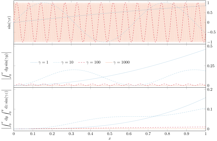
Fig. 1: Upper panel: the oscillating function sin(γx)𝛾𝑥\sin(\gamma x), for γ=1,10,100𝛾110100\gamma=1,10,100 and 100010001000. It is evident that as γ𝛾\gamma increases, the function oscillates more rapidly, crossing the horizontal axis more times per unit interval. Middle panel: the integral of the functions in the upper panel, of the form |(1/γ)(1cos(γx))|1𝛾1𝛾𝑥\left|(1/\gamma)(1-\cos(\gamma x))\right|, for the same values of γ𝛾\gamma. Lower panel: the double integral of the functions in the upper panel. As we can see, both graphically and analytically, as γ𝛾\gamma increases, the maxima of the integrals become smaller, and their amplitude decreases as 1/γ1𝛾1/\gamma. This allows us to neglect terms with γ103greater-than-or-equivalent-to𝛾superscript103\gamma\gtrsim 10^{3} when compared to terms where γ1similar-to𝛾1\gamma\sim 1.
dω^dx^=l,m(Almcos(lx^ω^+mωrx^ϵ)+Blmsin(lx^ω^+mωrx^ϵ))+𝒪(ϵ),d^𝜔d^𝑥subscript𝑙𝑚subscript𝐴𝑙𝑚𝑙^𝑥^𝜔𝑚subscript𝜔𝑟^𝑥italic-ϵsubscript𝐵𝑙𝑚𝑙^𝑥^𝜔𝑚subscript𝜔𝑟^𝑥italic-ϵ𝒪italic-ϵ\displaystyle\begin{split}\frac{\mathop{}\!\mathrm{d}\hat{\omega}}{\mathop{}\!\mathrm{d}\hat{x}}=\sum_{l,\,m}&\left(A_{lm}\cos\!\Bigg{(}\!l\hat{x}\hat{\omega}+\frac{m\omega_{r}\hat{x}}{\sqrt{\epsilon}}\!\Bigg{)}\vphantom{\Bigg{[}\Bigg{]}^{\!\!\!2\,}}\right.\\ &\left.\vphantom{\Bigg{[}\Bigg{]}^{\!\!\!2\,}}\!\!+B_{lm}\sin\!\Bigg{(}\!l\hat{x}\hat{\omega}+\frac{m\omega_{r}\hat{x}}{\sqrt{\epsilon}}\!\Bigg{)}\!\!\right)\!+\mathcal{O}\!\left(\epsilon\right),\end{split} (10)
d2ϕ^dx^2=l,m(Clmcos(lϕ^+mϕ^rϵ)+Dlmsin(lϕ^+mϕ^rϵ))+𝒪(ϵ).superscriptd2^italic-ϕdsuperscript^𝑥2subscript𝑙𝑚subscript𝐶𝑙𝑚𝑙^italic-ϕ𝑚subscript^italic-ϕ𝑟italic-ϵsubscript𝐷𝑙𝑚𝑙^italic-ϕ𝑚subscript^italic-ϕ𝑟italic-ϵ𝒪italic-ϵ\displaystyle\begin{split}\frac{\mathop{}\!\mathrm{d}^{2}\hat{\phi}}{\mathop{}\!\mathrm{d}\hat{x}^{2}}=\sum_{l,\,m}&\left(C_{lm}\cos\!\left(\!l\hat{\phi}+\frac{m\hat{\phi}_{r}}{\sqrt{\epsilon}}\!\right)\vphantom{\Bigg{[}\Bigg{]}^{\!\!\!2\,}}\right.\\ &\left.\vphantom{\Bigg{[}\Bigg{]}^{\!\!\!2\,}}\!\!\!+D_{lm}\sin\!\Bigg{(}\!l\hat{\phi}+\frac{m\hat{\phi}_{r}}{\sqrt{\epsilon}}\!\Bigg{)}\!\!\right)\!+\mathcal{O}\!\left(\epsilon\right).\end{split} (11)

For any non-zero value of the index m𝑚m, corrections to the frequency or phase equations are of the form cos(γx+δ)𝛾𝑥𝛿\cos(\gamma x+\delta), which oscillate rapidly owing to the γϵ1/2103similar-to𝛾superscriptitalic-ϵ12similar-tosuperscript103\gamma\sim\epsilon^{-\nicefrac{{1}}{{2}}}\sim 10^{3} factor both on resonance and away from it (and therefore will average out to zero over the timescales under consideration — this is illustrated in Figure 1). Hence, the correction to the first order solution of the phase equation is of the form (1/γ2)cos(γx+δ)1superscript𝛾2𝛾𝑥𝛿(1/\gamma^{2})\cos(\gamma x+\delta) and that of the frequency equation is (1/γ)sin(γx+δ)1𝛾𝛾𝑥𝛿(1/\gamma)\sin(\gamma x+\delta). These are terms of order ϵitalic-ϵ\epsilon and ϵ1/2superscriptitalic-ϵ12\epsilon^{\nicefrac{{1}}{{2}}}, respectively. Hence, we can perform an expansion to establish that they are corrections of higher order in the mass ratio and hence can be ignored at the same level as the other higher order in mass ratio terms that we have omitted. We can therefore consider only terms with m=0𝑚0m=0, and relabel the remaining modes by n𝑛n, obtaining

dω^dx^d^𝜔d^𝑥\displaystyle\frac{\mathop{}\!\mathrm{d}\hat{\omega}}{\mathop{}\!\mathrm{d}\hat{x}} =n(Ancos(nx^ω^)+Bnsin(nx^ω^))+𝒪(ϵ)absentsubscript𝑛subscript𝐴𝑛𝑛^𝑥^𝜔subscript𝐵𝑛𝑛^𝑥^𝜔𝒪italic-ϵ\displaystyle=\sum_{n}\left(\!A_{n}\cos\left(n\hat{x}\hat{\omega}\right)\!+\!B_{n}\sin\left(n\hat{x}\hat{\omega}\right)\!\!\vphantom{\Big{(}\Big{)}^{\!\!\!2\,}}\right)\!+\mathcal{O}\!\left(\epsilon\right) (12)
d2ϕ^dx^2superscriptd2^italic-ϕdsuperscript^𝑥2\displaystyle\frac{\mathop{}\!\mathrm{d}^{2}\hat{\phi}}{\mathop{}\!\mathrm{d}\hat{x}^{2}} =n(Cncos(nϕ^)+Dnsin(nϕ^))+𝒪(ϵ).absentsubscript𝑛subscript𝐶𝑛𝑛^italic-ϕsubscript𝐷𝑛𝑛^italic-ϕ𝒪italic-ϵ\displaystyle=\sum_{n}\left(\!C_{n}\cos\!\left(n\hat{\phi}\right)\!+\!D_{n}\sin\!\left(n\hat{\phi}\right)\!\!\vphantom{\Big{(}\Big{)}^{\!\!\!2\,}}\right)\!+\mathcal{O}\!\left(\epsilon\right). (13)

We combine the two oscillating modes together, and this introduces a phase to the oscillating term. This could sometimes be set to 0 by suitable choice of initial coordinates, however it is not always possible, since the resonance phase depends on the prior evolution of the binary system. To preserve generality of the problem, we will include it in our equations. The presence of phase does not complicate the method of solution, only brings in additional terms, as we will demonstrate later in Section IV.

dω^dx^d^𝜔d^𝑥\displaystyle\frac{\mathop{}\!\mathrm{d}\hat{\omega}}{\mathop{}\!\mathrm{d}\hat{x}} =n𝒜ncos(nx^ω^δχn)+𝒪(ϵ)absentsubscript𝑛subscript𝒜𝑛𝑛^𝑥^𝜔𝛿subscript𝜒𝑛𝒪italic-ϵ\displaystyle=\sum_{n}\,\mathcal{A}_{n}\cos\left(n\hat{x}\hat{\omega}-\delta\chi_{n}\right)+\mathcal{O}\!\left(\epsilon\right) (14)
d2ϕ^dx^2superscriptd2^italic-ϕdsuperscript^𝑥2\displaystyle\frac{\mathop{}\!\mathrm{d}^{2}\hat{\phi}}{\mathop{}\!\mathrm{d}\hat{x}^{2}} =nncos(nϕ^δψn)+𝒪(ϵ),absentsubscript𝑛subscript𝑛𝑛^italic-ϕ𝛿subscript𝜓𝑛𝒪italic-ϵ\displaystyle=\sum_{n}\,\mathcal{B}_{n}\cos\!\left(n\hat{\phi}-\delta\psi_{n}\right)\!+\mathcal{O}\!\left(\epsilon\right), (15)

where

𝒜n=An2+Bn2,n=Cn2+Dn2,δχn=arctan(BnAn)andδψn=arctan(DnCn).formulae-sequencesubscript𝒜𝑛superscriptsubscript𝐴𝑛2superscriptsubscript𝐵𝑛2formulae-sequencesubscript𝑛superscriptsubscript𝐶𝑛2superscriptsubscript𝐷𝑛2𝛿subscript𝜒𝑛subscript𝐵𝑛subscript𝐴𝑛and𝛿subscript𝜓𝑛subscript𝐷𝑛subscript𝐶𝑛\displaystyle\begin{split}&\quad\quad\mathcal{A}_{n}=\sqrt{\vphantom{|}A_{n}^{2}+B_{n}^{2}}\,,\;\;\;\mathcal{B}_{n}=\sqrt{\vphantom{|}C_{n}^{2}+D_{n}^{2}}\,,\\ &\delta\chi_{n}=\arctan\!\left(\!\frac{B_{n}}{A_{n}}\!\right)\;\;\text{and}\;\;\;\delta\psi_{n}=\arctan\!\left(\!\frac{D_{n}}{C_{n}}\!\right).\end{split} (16)

Finally, we split the first term from the sum, n=0𝑛0n=0, which is constant (with respect to time or phase, respectively):

dω^dx^d^𝜔d^𝑥\displaystyle\frac{\mathop{}\!\mathrm{d}\hat{\omega}}{\mathop{}\!\mathrm{d}\hat{x}}\! =𝒜0cos(δχ0)+n>0𝒜ncos(nx^ω^δχn)+𝒪(ϵ)absentsubscript𝒜0𝛿subscript𝜒0subscript𝑛0subscript𝒜𝑛𝑛^𝑥^𝜔𝛿subscript𝜒𝑛𝒪italic-ϵ\displaystyle=\!\mathcal{A}_{0}\cos(\delta\chi_{0})+\!\sum_{n>0}\!\mathcal{A}_{n}\cos\!\left(n\hat{x}\hat{\omega}\!-\!\delta\chi_{n}\right)+\mathcal{O}\!\left(\epsilon\right) (17)
d2ϕ^dx^2superscriptd2^italic-ϕdsuperscript^𝑥2\displaystyle\frac{\mathop{}\!\mathrm{d}^{2}\hat{\phi}}{\mathop{}\!\mathrm{d}\hat{x}^{2}}\! =0cos(δψ0)+n>0ncos(nϕ^δψn)+𝒪(ϵ)absentsubscript0𝛿subscript𝜓0subscript𝑛0subscript𝑛𝑛^italic-ϕ𝛿subscript𝜓𝑛𝒪italic-ϵ\displaystyle=\!\mathcal{B}_{0}\cos(\delta\psi_{0})+\!\sum_{n>0}\!\mathcal{B}_{n}\cos\!\left(n\hat{\phi}\!-\!\delta\psi_{n}\right)\!+\mathcal{O}\!\left(\epsilon\right) (18)

and make a suitable, final change of variables:

ω=(𝒜0cos(δχ0))1/2ω^xω=(𝒜0cos(δχ0))1/2x^𝜔superscriptsubscript𝒜0𝛿subscript𝜒012^𝜔subscript𝑥𝜔superscriptsubscript𝒜0𝛿subscript𝜒012^𝑥\displaystyle\begin{split}\omega&=\big{(}\mathcal{A}_{0}\cos(\delta\chi_{0})\big{)}^{-\nicefrac{{1}}{{2}}}\>\hat{\omega}\\ x_{\omega}&=\big{(}\mathcal{A}_{0}\cos(\delta\chi_{0})\big{)}^{\nicefrac{{1}}{{2}}}\>\hat{x}\end{split}\quad\quad in eq. (17)

and

xϕ=(0cos(δψ0))1/2x^ϕ=ϕ^subscript𝑥italic-ϕsuperscriptsubscript0𝛿subscript𝜓012^𝑥italic-ϕ^italic-ϕ\displaystyle\begin{split}x_{\phi}&=\big{(}\mathcal{B}_{0}\cos(\delta\psi_{0})\big{)}^{\nicefrac{{1}}{{2}}}\>\hat{x}\\ \phi&=\hat{\phi}\end{split}\quad\quad in eq. (18)

to bring the equations to their most simplified form:

ωsuperscript𝜔\displaystyle\omega^{\prime} =1+nκncos(nxωωδχn)absent1subscript𝑛subscript𝜅𝑛𝑛subscript𝑥𝜔𝜔𝛿subscript𝜒𝑛\displaystyle=1+\sum_{n}\kappa_{n}\cos\big{(}nx_{\omega}\,\omega-\delta\chi_{n}\big{)} (19a)
ϕ′′superscriptitalic-ϕ′′\displaystyle\phi^{\prime\prime} =1+nλncos(nϕδψn),absent1subscript𝑛subscript𝜆𝑛𝑛italic-ϕ𝛿subscript𝜓𝑛\displaystyle=1+\sum_{n}\lambda_{n}\cos\big{(}n\phi-\delta\psi_{n}\big{)}, (19b)

where κn=(𝒜n/𝒜0)sec(δχ0)subscript𝜅𝑛subscript𝒜𝑛subscript𝒜0𝛿subscript𝜒0\kappa_{n}\!=(\mathcal{A}_{n}/\mathcal{A}_{0})\sec(\delta\chi_{0}) and λn=(n/0)sec(δψ0)subscript𝜆𝑛subscript𝑛subscript0𝛿subscript𝜓0\lambda_{n}\!=(\mathcal{B}_{n}/\mathcal{B}_{0})\sec(\delta\psi_{0}) are in principle known constants, dependent on the orbital parameters at resonance, prime denotes a derivative with respect to the rescaled time x𝑥x and the quantities {δχi}𝛿subscript𝜒𝑖\{\delta\chi_{i}\} and {δϕj}𝛿subscriptitalic-ϕ𝑗\{\delta\phi_{j}\} are constants. The sums over n𝑛n run from 1 to \infty, however we will later consider finite number of modes on the right-hand side. In order to achieve convergence when solving these equations, we need to make the assumption that the series {κn}subscript𝜅𝑛\{\kappa_{n}\} and {λn}subscript𝜆𝑛\{\lambda_{n}\} follow a power law of the form nαsuperscript𝑛𝛼n^{-\alpha}, with α2greater-than-or-equivalent-to𝛼2\alpha\gtrsim 2, this is discussed in detail in Section IV.1. In this paper, we are attempting to find solutions to eqs. (19a) and (19b) in increasing order of complexity. It is worth noting that while one of them is a first-order equation, the other is of second order. They derive from equivalent representations of the geodesics, however the first and second order equations are no longer equivalent, because they make different assumptions about the expansion of the self-force.

Before proposing the respective solutions, we will focus on presenting an alternative approach to describing the behaviour of an emri near resonance.

III Two-timescale approach

An alternative approach to describing the transition of emris through resonances was first suggested by (Hinderer and Flanagan, 2008), and is often called the “two-timescale method” since it differentiates between processes which occur on short (orbital) timescales, and those happening on long (orbit evolution) timescales. A good overview is offered by Kevorkian (1987).

Here we will present this method as described by van de Meent (2014), while it is also advisable that the reader consults Berry (2013), and the original article by Hinderer and Flanagan (2008). Again, we consider the motion of a compact object spiralling towards a supermassive black hole, and describe the evolution in terms of the perturbative parameter, the mass ratio ϵitalic-ϵ\epsilon. At leading order, we recover the geodesic equations of motion, as before. At next order, we need to introduce corrections due to the self-force acting on the compact object, in analogy with eq. (3) in the instantaneous frequency approach:

dJμdτdsubscript𝐽𝜇d𝜏\displaystyle\frac{\mathop{}\!\mathrm{d}J_{\mu}}{\mathop{}\!\mathrm{d}\tau} =ϵμ(𝐪,𝐅)+𝒪(ϵ2)absentitalic-ϵsubscript𝜇𝐪𝐅𝒪superscriptitalic-ϵ2\displaystyle=\epsilon\,\mathcal{I}_{\mu}(\mathbf{q},\mathbf{F})+\mathcal{O}\!\left(\epsilon^{2}\right) (20)

While the equations in Berry (2013) are presented in terms of the Mino time λ𝜆\lambda (Mino, 2003), we can map λ𝜆\lambda to the proper time τ𝜏\tau through a function involving the coordinates of the compact object. We can absorb this dependence into the functions μsubscript𝜇\mathcal{I}_{\mu} on right-hand side of eq. (20) and work in terms of the proper time. As before, we can exchange the integrals of the motion 𝐉𝐉\mathbf{J} in favour of the fundamental frequencies 𝝎𝝎\bm{\omega}, since mappings between these exist (Schmidt, 2002), albeit not invertable over the entire domain. Further we can implicitly write the self-force as a function of the coordinates and their corresponding frequencies (cf. eq. (5)) to obtain:

dωμdτdsubscript𝜔𝜇d𝜏\displaystyle\frac{\mathop{}\!\mathrm{d}\omega_{\mu}}{\mathop{}\!\mathrm{d}\tau} =ϵ𝒥μ(𝐪,𝐉)+𝒪(ϵ2)absentitalic-ϵsubscript𝒥𝜇𝐪𝐉𝒪superscriptitalic-ϵ2\displaystyle=\epsilon\,\mathcal{J}_{\mu}(\mathbf{q},\mathbf{J})+\mathcal{O}\!\left(\epsilon^{2}\right) (21)

Similarly, the action-angle variables evolve as per eq. (4):

dqμdτ=ωμ(𝐉)+ϵ𝒦μ(𝐪,𝐉)+𝒪(ϵ2).dsubscript𝑞𝜇d𝜏subscript𝜔𝜇𝐉italic-ϵsubscript𝒦𝜇𝐪𝐉𝒪superscriptitalic-ϵ2\displaystyle\frac{\mathop{}\!\mathrm{d}q_{\mu}}{\mathop{}\!\mathrm{d}\tau}=\omega_{\mu}\left(\mathbf{J}\right)+\epsilon\,\mathcal{K}_{\mu}(\mathbf{q},\mathbf{J})+\mathcal{O}\!\left(\epsilon^{2}\right). (22)

We construct the resonant frequency ν¯=l0ωrm0ωθ¯𝜈subscript𝑙0subscript𝜔𝑟subscript𝑚0subscript𝜔𝜃\bar{\nu}=l_{0}\,\omega_{r}-m_{0}\,\omega_{\theta}, and the corresponding action-angle variable combination q¯=l0qrm0qθ¯𝑞subscript𝑙0subscript𝑞𝑟subscript𝑚0subscript𝑞𝜃\bar{q}=l_{0}\,q_{r}-m_{0}\,q_{\theta}. ν¯¯𝜈\bar{\nu} is the analogous variable to ω¯¯𝜔\bar{\omega} in Section II, but we use a different notation here to differentiate between the two methods. Again, we ignore the third fundamental frequency ωϕsubscript𝜔italic-ϕ\omega_{\phi}, since the motion is axisymmetric. Let J¯¯𝐽\bar{J} denote the action conjugate to q¯¯𝑞\bar{q}, which can be mapped to ν¯¯𝜈\bar{\nu}. Further, let us rescale the proper time to write xν=ϵτsubscript𝑥𝜈italic-ϵ𝜏x_{\nu}=\sqrt{\epsilon}\,\tau. We now expand the frequency and coordinate variables in powers of ϵitalic-ϵ\epsilon:

ν¯(xν,ϵ)¯𝜈subscript𝑥𝜈italic-ϵ\displaystyle\bar{\nu}\left(x_{\nu},\epsilon\right) =ν¯0+ϵ1/2ν¯1(xν)+𝒪(ϵ2)absentsubscript¯𝜈0superscriptitalic-ϵ12subscript¯𝜈1subscript𝑥𝜈𝒪superscriptitalic-ϵ2\displaystyle=\bar{\nu}_{0}+\epsilon^{\nicefrac{{1}}{{2}}}\,\bar{\nu}_{1}(x_{\nu})+\mathcal{O}\!\left(\epsilon^{2}\right) (23a)
q¯(xν,ϵ)¯𝑞subscript𝑥𝜈italic-ϵ\displaystyle\bar{q}\left(x_{\nu},\epsilon\right) =q¯0(xν)+ϵ1/2q¯1(xν)+𝒪(ϵ2).absentsubscript¯𝑞0subscript𝑥𝜈superscriptitalic-ϵ12subscript¯𝑞1subscript𝑥𝜈𝒪superscriptitalic-ϵ2\displaystyle=\bar{q}_{0}(x_{\nu})+\epsilon^{\nicefrac{{1}}{{2}}}\,\bar{q}_{1}(x_{\nu})+\mathcal{O}\!\left(\epsilon^{2}\right). (23b)

Plugging these power laws into the (averaged) evolution equations (21) and (22) yields the resonance equations:

dν¯1dxνdsubscript¯𝜈1dsubscript𝑥𝜈\displaystyle\frac{\mathop{}\!\mathrm{d}\bar{\nu}_{1}}{\mathop{}\!\mathrm{d}x_{\nu}} =𝒥¯(q¯,J¯)+𝒪(ϵ)absent¯𝒥¯𝑞¯𝐽𝒪italic-ϵ\displaystyle=\bar{\mathcal{J}}\!\left(\bar{q},\bar{J}\right)+\mathcal{O}\!\left(\epsilon\right) (24a)
dq¯0dxνdsubscript¯𝑞0dsubscript𝑥𝜈\displaystyle\frac{\mathop{}\!\mathrm{d}\bar{q}_{0}}{\mathop{}\!\mathrm{d}x_{\nu}} =ν¯1(xν)+𝒪(ϵ).absentsubscript¯𝜈1subscript𝑥𝜈𝒪italic-ϵ\displaystyle=\bar{\nu}_{1}(x_{\nu})+\mathcal{O}\!\left(\epsilon\right). (24b)

This relays the leading terms in the expansions (23). Further members of the series {ν¯n}subscript¯𝜈𝑛\{\bar{\nu}_{n}\} and {q¯n}subscript¯𝑞𝑛\{\bar{q}_{n}\} can be found iteratively by substituting the results from eqs. (24) back into the resonance evolution equations.

Refer to caption
Fig. 2: Visualisation of several types of series for the mode parameters ki={κi,λi}subscript𝑘𝑖subscript𝜅𝑖subscript𝜆𝑖k_{i}=\{\kappa_{i},\lambda_{i}\}. For each of them, we take 4 different values of the initial parameter: k1=0.1subscript𝑘10.1k_{1}=0.1 (          ), k2=0.05subscript𝑘20.05k_{2}=0.05 (    ), k3=0.01subscript𝑘30.01k_{3}=0.01 (  ), and k4=0.005subscript𝑘40.005k_{4}=0.005 (   ). Left panel: Logarithmic progression with base 2, kn=k1/log2(n+1)subscript𝑘𝑛subscript𝑘1subscript2𝑛1k_{n}=k_{1}/\log_{2}(n+1), which is too slow to satisfy our conditions for convergence. Centre panel: Power law kn=k1/nαsubscript𝑘𝑛subscript𝑘1superscript𝑛𝛼k_{n}=k_{1}/n^{\alpha}, with α=2.5𝛼2.5\alpha=2.5, as suggested by (Drasco and Hughes, 2006) (the lower bound is α2greater-than-or-equivalent-to𝛼2\alpha\gtrsim 2). Right panel: Exponential series kn=k1/2n1subscript𝑘𝑛subscript𝑘1superscript2𝑛1k_{n}=k_{1}/2^{n-1}. It is expected that in reality, this progression will start as a power law (centre panel) and will gradually evolve into an exponential series for large values of n𝑛n (right panel). This data is represented numerically in Table 1.

In Flanagan and Hinderer (2012), eq. (23a) was further simplified by expanding ν¯1subscript¯𝜈1\bar{\nu}_{1} as a series in ϵxνitalic-ϵsubscript𝑥𝜈\sqrt{\epsilon}\,x_{\nu}. The leading term is then ν1(xνx0)subscript𝜈1subscript𝑥𝜈subscript𝑥0\nu_{1}(x_{\nu}-x_{0}) for a constant ν1subscript𝜈1\nu_{1}. Proceeding with the two timescale expansion then yields a result accurate to first order in the resonant modification, {λn}subscript𝜆𝑛\{\lambda_{n}\}, which agrees with the result obtained from the asymptotic Fourier series approach in Gair, Yunes, and Bender (2012). Corrections at higher order in λnsubscript𝜆𝑛\lambda_{n}, but leading order in mass ratio, cannot be found in this way, since the assumption of a linearly evolving frequency is only valid close to the resonance point. The two-timescale approach can be extended to higher order by using a less restrictive ansatz for ν¯1subscript¯𝜈1\bar{\nu}_{1}, which is given implicitly by eqs (23) and (25) in van de Meent (2014). Explicit solutions to higher order in the resonant modification at leading order in mass ratio have not been computed in the two-timescale approach. However, we anticipate that these will agree with the phase version of the asymptotic Fourier series approach. The purpose of this paper is to extend previous calculations to higher order in resonant modification and to include multiple modes in the resonance. To do this we will use the asymptotic Fourier series approach and this will be the focus for the remainder of this paper.

IV Solutions of the resonance equations

We are now in a position to solve the instantaneous frequency approach equations that we derived earlier in Section II. Evolution of the action-angle coordinates according to the instantaneous frequency of the system yields the 2 non-linear differential eqs. (19a) and (19b). Due to the constant additive term on their right-hand sides, these equations cannot be solved exactly, and therefore we need to come up with an alternative approach. In this Section we propose solutions to these equations in an increasing order of complexity. Solutions for the single-mode versions of eqs. (19) are provided in Gair, Yunes, and Bender (2012), we will start by re-deriving those to depict how the order-by-order solution algorithm works. Following this, we relax the assumptions which have been considered in Gair, Yunes, and Bender (2012) in order to build up solutions to the generalised source equations.

IV.1 Regime and domain of the variables

Before attempting to solve the resonance equations, we need to specify their domains and any special limits we are taking. The time parameters x{ω,ϕ,ν}subscript𝑥𝜔italic-ϕ𝜈x_{\{\omega,\,\phi,\,\nu\}} range from -\infty to ++\infty, however we are interested in the vicinity of x=0𝑥0x=0 as this is when resonance occurs, hence where we have specified the initial conditions. In this notation, -\infty corresponds to times long before resonance, and ++\infty to times when the resonance has had an effect on the orbit. Therefore, in solving these equations, we will consider definite integrals of the form 0xdx¯superscriptsubscript0𝑥differential-d¯𝑥\int_{0}^{x}\mathop{}\!\mathrm{d}\bar{x}, where x𝑥x can take large positive or negative values. Since the equations are not coupled, and each rescaled time variable appears in the differential equation for its corresponding quantity, we will drop the subscripts on x𝑥x, and will keep track of them by the subject of the equation we are solving.

More attention needs to be devoted to the fractional resonance modifications, κisubscript𝜅𝑖\kappa_{i} and λjsubscript𝜆𝑗\lambda_{j}, which are themselves functions of the orbital parameters. As discussed in Gair, Yunes, and Bender (2012), if these modifications are of order unity, there can be a qualitative difference in the on-resonance behaviour, with the possibility of sustained resonances. These were explored in more detail in van de Meent (2014). A complete study of the size of on-resonance flux modifications has not yet been carried out. Some insight on the likely size of these corrections can be obtained by studying solutions to the Teukolsky equation, which provide a decomposition of the off-resonance energy flux into different Fourier modes. Such results can be found in Drasco and Hughes (2006). Section I C of that paper indicates that the size of the terms in this decomposition initially follows a power law of the form nαsimilar-toabsentsuperscript𝑛𝛼\sim n^{-\alpha} before eventually falling off exponentially (see Figure 2 and Table 1 for an illustration different rates of fall off). From Fig. 3 of that paper it appears that α2greater-than-or-equivalent-to𝛼2\alpha\gtrsim 2 for all n𝑛n, but as a lower limit in our calculations we will use the value of α=5/2𝛼52\alpha=5/2. Drasco and Hughes (2006) also indicate that the size of the first term in the series is less than unity, and in fact of order κ1λ10.1similar-tosubscript𝜅1subscript𝜆1similar-to0.1\kappa_{1}\sim\lambda_{1}\sim 0.1. This implies that the resonance is likely to be “weak”, but the Teukolsky results do not directly give the size of the on-resonance flux change. The size of the resonance effect was assessed more carefully in flanaganhughesruangsri2012, who computed the flux change for a number of different resonances for a few systems and found that the resonant flux change was only 1%similar-toabsentpercent1\sim 1\% in all cases. This also suggests that κ1subscript𝜅1\kappa_{1} and λ1subscript𝜆1\lambda_{1} are small, typically 0.01similar-toabsent0.01\sim 0.01. Based on this evidence it seems unlikely that strong resonances will occur in practice and so in this article we focus on the weak resonance case with κ11much-less-thansubscript𝜅11\kappa_{1}\ll 1, which will allow us to perform an expansion in κ1subscript𝜅1\kappa_{1}. However, we should note that flanaganhughesruangsri2012 did not thoroughly explore the resonance parameter space and so it is still possible that there are regions of parameter space where strong sustained resonances may exist. If this is possible, it would be very interesting, as discussed in detail in van de Meent (2014).

Regarding the other relevant parameters, the mass-ratio ϵitalic-ϵ\epsilon is typically in the range 106103similar-toabsentlimit-fromsuperscript106similar-tosuperscript103\sim{10^{-6}}-\sim{10^{-3}}. The quantity ϵ1/2superscriptitalic-ϵ12\epsilon^{1/2} is therefore 𝒪(103101.5)𝒪superscript103superscript101.5\mathcal{O}\!\left(10^{-3}-10^{-1.5}\right). The phases on resonance, δχi𝛿subscript𝜒𝑖\delta\chi_{i} and δψj𝛿subscript𝜓𝑗\delta\psi_{j}, are constants in the range [0,2π)02𝜋[0,2\pi), which depend only on the coefficients of the Fourier series in eqs. (6) and (7), and the index n𝑛n.

Refer to caption
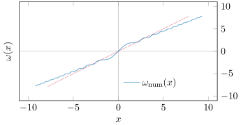
Fig. 3: Numerical solution of the equation ω=1+κcos(xω)superscript𝜔1𝜅𝑥𝜔\omega^{\prime}=1+\kappa\cos\left(x\omega\right), with κ=0.9𝜅0.9\kappa=0.9, an exaggerated value is used to demonstrate the notable features of the solution, namely the slope and the decaying oscillations. The initial condition ω(0)𝜔0\omega(0) depends on the initial phase of the resonance, and has been set to 1 here. The line ω(x)=1+x𝜔𝑥1𝑥\omega(x)=1+x is plotted (in red dots) for reference.

IV.2 Frequency resonance equation

Consider the generalised frequency resonance equation:

ωsuperscript𝜔\displaystyle\omega^{\prime} =1+nκncos(nxωωδχn),absent1subscript𝑛subscript𝜅𝑛𝑛subscript𝑥𝜔𝜔𝛿subscript𝜒𝑛\displaystyle=1+\sum_{n}\kappa_{n}\cos\big{(}nx_{\omega}\,\omega-\delta\chi_{n}\big{)}, (19a)

where prime denotes differentiation with respect to the rescaled time parameter xωsubscript𝑥𝜔x_{\omega}. Before attempting to solve this equation in the general case, we consider only the single oscillatory mode (n=1𝑛1n=1, besides the n=0𝑛0n=0 mode) on the right-hand side, and as agreed, drop the subscript on x𝑥x. The resulting problem is not much simpler to solve, however it will provide useful insight about the method:

ω(x)=1+κcos(xω),superscript𝜔𝑥1𝜅𝑥𝜔\displaystyle\omega^{\prime}(x)=1+\kappa\cos\left(x\omega\right), (25)

where κκ0𝜅subscript𝜅0\kappa\equiv\kappa_{0}. Inspired by the numerical solution of eq. (25), shown in Fig. (3), we split the solution in two parts: the first for the region where the oscillations are still growing, and the second where the oscillations gradually decay. After we establish appropriate solutions to eq. (25) in each of these regions, we will come up with a way to match them on the boundary region.

Let us initially look for a solution in the κ|x|1much-less-than𝜅𝑥1\kappa|x|\ll 1 region. That is, find an expansion of the frequency ω𝜔\omega as a function of x𝑥x in the region immediately around x=0𝑥0x=0, in powers of the fractional resonance modification κ𝜅\kappa:

ω(x)=n=0κnϖn(x).𝜔𝑥superscriptsubscript𝑛0superscript𝜅𝑛subscriptitalic-ϖ𝑛𝑥\displaystyle\omega(x)=\sum_{n=0}^{\infty}\kappa^{n}\varpi_{n}(x). (26)
Refer to caption
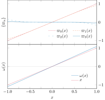
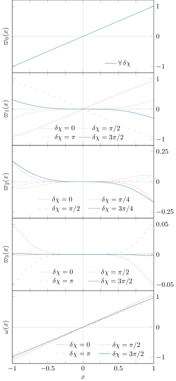
Fig. 4: Analytical solution to the frequency equation for |x|<1𝑥1|x|<1. Top panel: The solutions at each order from 0 to 3 inclusive, plotted as a function of x𝑥x. Bottom panel: The combined solution at third order, eq. (36).

We remind ourselves that the parameter κ1much-less-than𝜅1\kappa\ll 1, as per Section IV.1. In order to find explicit forms of the functions {ϖn}subscriptitalic-ϖ𝑛\{\varpi_{n}\}, we substitute the expansion (26) in eq. (25) and proceed to match terms on both sides. The results we now derive are plotted in Figure 4. At lowest order, we disregard all terms of 𝒪(κ)𝒪𝜅\mathcal{O}\!\left(\kappa\right) and higher:

ϖ0(x)=1ϖ0(x)=x,formulae-sequencesuperscriptsubscriptitalic-ϖ0𝑥1subscriptitalic-ϖ0𝑥𝑥\displaystyle\varpi_{0}^{\prime}(x)=1\quad\Leftrightarrow\quad\varpi_{0}(x)=x, (27)

where it is important to note that the integration has been carried out between 0 and x𝑥x. Further terms in the series (26) will be reduced by one or more factors of κ1much-less-than𝜅1\kappa\ll 1, hence we can treat them as a perturbation to ϖ0(x)subscriptitalic-ϖ0𝑥\varpi_{0}(x):

n=1κnϖn(x)=κcos[x2+n=1κnxϖn(x)].superscriptsubscript𝑛1superscript𝜅𝑛subscriptitalic-ϖ𝑛𝑥𝜅superscript𝑥2superscriptsubscript𝑛1superscript𝜅𝑛𝑥subscriptitalic-ϖ𝑛𝑥\displaystyle\sum_{n=1}^{\infty}\kappa^{n}\varpi_{n}(x)=\kappa\cos\!\left[x^{2}+\sum_{n=1}^{\infty}\kappa^{n}x\,\varpi_{n}(x)\right]. (28)

At the next higher order we find the equation for ϖ1(x)subscriptitalic-ϖ1𝑥\varpi_{1}(x):

κϖ1(x)+𝒪(κ2)=κcos(x2)+𝒪(κ2).𝜅superscriptsubscriptitalic-ϖ1𝑥𝒪superscript𝜅2𝜅superscript𝑥2𝒪superscript𝜅2\displaystyle\kappa\varpi_{1}^{\prime}(x)+\mathcal{O}\!\left(\kappa^{2}\right)=\kappa\cos\!\left(x^{2}\right)+\mathcal{O}\!\left(\kappa^{2}\right). (29)

integrating the right-hand side yields the solution:

ϖ1(x)=0xdycos(y2)=2π2C(2xπ),subscriptitalic-ϖ1𝑥superscriptsubscript0𝑥differential-d𝑦superscript𝑦22𝜋2𝐶2𝑥𝜋\displaystyle\varpi_{1}(x)=\int_{0}^{x}\mathop{}\!\mathrm{d}y\cos\!\left(y^{2}\right)=\frac{\sqrt{2\pi}}{2}\,C\!\left(\!\frac{\sqrt{2}\,x}{\sqrt{\pi}}\!\right), (30)

where C()𝐶C(\bullet) is the Fresnel cosine integral (see Appendix D and Figure 25 for details). At 𝒪(κ2)𝒪superscript𝜅2\mathcal{O}\!\left(\kappa^{2}\right), we find:

ϖ2(x)=π2xsin(x2)C(2xπ).superscriptsubscriptitalic-ϖ2𝑥𝜋2𝑥superscript𝑥2𝐶2𝑥𝜋\displaystyle\varpi_{2}^{\prime}(x)=-\,\frac{\sqrt{\pi}}{\sqrt{2}}\,x\,\sin\!\left(x^{2}\right)C\!\left(\!\frac{\sqrt{2}\,x}{\sqrt{\pi}}\!\right). (31)

Solving this differential equation (which also involves a simple integration by parts) provides the solution:

ϖ2(x)=2π4cos(x2)C(2xπ)π8C(4xπ)x4.subscriptitalic-ϖ2𝑥2𝜋4superscript𝑥2𝐶2𝑥𝜋𝜋8𝐶4𝑥𝜋𝑥4\displaystyle\varpi_{2}(x)=\frac{\sqrt{2\pi}}{4}\cos\!\big{(}x^{2}\big{)}C\!\left(\!\frac{\sqrt{2}\,x}{\sqrt{\pi}}\!\right)\!-\frac{\sqrt{\pi}}{8}\,C\!\left(\!\frac{\sqrt{4}\,x}{\sqrt{\pi}}\!\right)\!-\frac{x}{4}.

It is obvious that with increasing order the functional form of ϖn(x)subscriptitalic-ϖ𝑛𝑥\varpi_{n}(x) become more and more involved. It will become apparent later on why we do not need solutions at 𝒪(κ4)𝒪superscript𝜅4\mathcal{O}\!\left(\kappa^{4}\right) and beyond. However, at third order, we find the following differential equation for the functional ϖ3(x)subscriptitalic-ϖ3𝑥\varpi_{3}(x).

Refer to caption
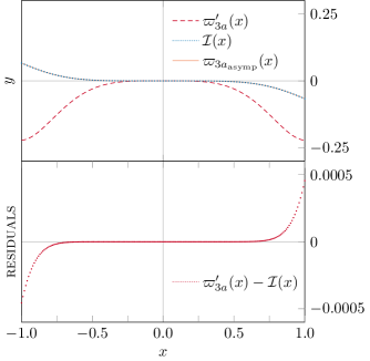
Fig. 5: Approximate integral of ϖ3a(x)superscriptsubscriptitalic-ϖ3𝑎𝑥\varpi_{3a}^{\prime}(x) near the origin. Top panel: The integrand, the numerical integral, and the approximation. Bottom panel: Residuals between the approximation and the numerical solution, showing the validity of eq. (34).
ϖ3(x)=π4x2cos(x2)C2(2xπ)xsin(x2)ϖ2(x).superscriptsubscriptitalic-ϖ3𝑥𝜋4superscript𝑥2superscript𝑥2superscript𝐶22𝑥𝜋𝑥superscript𝑥2subscriptitalic-ϖ2𝑥\displaystyle\varpi_{3}^{\prime}(x)=-\frac{\pi}{4}\,x^{2}\cos\!\left(x^{2}\right)C^{2}\!\!\left(\!\frac{\sqrt{2}\,x}{\sqrt{\pi}}\!\right)\!-x\sin\!\left(x^{2}\right)\varpi_{2}(x).

We divide ϖ3subscriptitalic-ϖ3\varpi_{3} into two parts, ϖ3(x)=ϖ3a(x)+ϖ3b(x)subscriptitalic-ϖ3𝑥subscriptitalic-ϖ3𝑎𝑥subscriptitalic-ϖ3𝑏𝑥\varpi_{3}(x)=\varpi_{3a}(x)+\varpi_{3b}(x), defined via the two differential equations:

ϖ3a(x)superscriptsubscriptitalic-ϖ3𝑎𝑥\displaystyle\varpi_{3a}^{\prime}(x) =π4x2cos(x2)C2(2xπ)absent𝜋4superscript𝑥2superscript𝑥2superscript𝐶22𝑥𝜋\displaystyle=-\frac{\pi}{4}\,x^{2}\cos\!\left(x^{2}\right)C^{2}\!\!\left(\!\frac{\sqrt{2}\,x}{\sqrt{\pi}}\!\right)\! (32a)
ϖ3b(x)superscriptsubscriptitalic-ϖ3𝑏𝑥\displaystyle\varpi_{3b}^{\prime}(x) =xsin(x2)ϖ2(x).absent𝑥superscript𝑥2subscriptitalic-ϖ2𝑥\displaystyle=-x\sin\!\left(x^{2}\right)\varpi_{2}(x). (32b)

Unfortunately, the term ϖ3a(x)subscriptitalic-ϖ3𝑎𝑥\varpi_{3a}(x) above is the only integral in our analysis which cannot be performed analytically. However, we can proceed by expanding the Fresnel term on the right hand side for small x𝑥x and integrating the resulting terms. We then define ϖ3aapprox(x)subscriptitalic-ϖ3subscript𝑎approx𝑥\varpi_{3a_{\rm approx}}(x) to be the terms arising from this integration, given analytically by eq. (34). This has the property ϖ3a(x)ϖ3aapprox(x)𝒪(x9)similar-tosuperscriptsubscriptitalic-ϖ3𝑎𝑥superscriptsubscriptitalic-ϖ3subscript𝑎approx𝑥𝒪superscript𝑥9\varpi_{3a}^{\prime}(x)-\varpi_{3a_{\rm approx}}^{\prime}(x)\sim\mathcal{O}\!\left(x^{9}\right) and hence ϖ3a(x)ϖ3aapprox(x)𝒪(x10)similar-tosubscriptitalic-ϖ3𝑎𝑥subscriptitalic-ϖ3subscript𝑎approx𝑥𝒪superscript𝑥10\varpi_{3a}(x)-\varpi_{3a_{\rm approx}}(x)\sim\mathcal{O}\!\left(x^{10}\right). Finally, we need to verify that this is a valid approximation; we can do this by tabulating the function

(x)=0xdyϖ3a(y)𝑥superscriptsubscript0𝑥differential-d𝑦superscriptsubscriptitalic-ϖ3𝑎𝑦\displaystyle\mathcal{I}(x)=\int_{0}^{x}\!\!\mathop{}\!\mathrm{d}y\,\varpi_{3a}^{\prime}(y) (33)

for values of x𝑥x between 11-1 and 1, and comparing this with our (approximate) analytical result for the integral, eq. (34). The integrand, both functions, and the residuals of the approximation are shown in Fig. 5.

The term in eq. (32b) can be integrated analytically, and the result is given by expression (35). Gathering the above results together, we can write down an approximate solution to the Frequency equation, which is given in eq. (36). We note that this is valid for κ|x|1much-less-than𝜅𝑥1\kappa|x|\ll 1 up to 𝒪(κ2)𝒪superscript𝜅2\mathcal{O}\!\left(\kappa^{2}\right), while the result for ϖ3(x)subscriptitalic-ϖ3𝑥\varpi_{3}(x) is only valid when |x|1much-less-than𝑥1|x|\ll 1. Later on, as the need arises, we will find a solution for ϖ3(x)subscriptitalic-ϖ3𝑥\varpi_{3}(x) which is valid in other regimes.

ϖ3aapprox(x)=332π64C(2xπ)3332xcos(x2)1116x3sin(x2)+740x5cos(x2)+120x7sin(x2)subscriptitalic-ϖ3subscript𝑎approx𝑥332𝜋64𝐶2𝑥𝜋3332𝑥superscript𝑥21116superscript𝑥3superscript𝑥2740superscript𝑥5superscript𝑥2120superscript𝑥7superscript𝑥2\displaystyle\begin{split}&\varpi_{3a_{\rm approx}}(x)=\frac{33\sqrt{2\pi}}{64}\,C\!\left(\!\frac{\sqrt{2}\,x}{\sqrt{\pi}}\!\right)\!-\frac{33}{32}\,x\cos\!\big{(}x^{2}\big{)}-\frac{11}{16}\,x^{3}\sin\!\big{(}x^{2}\big{)}+\frac{7}{40}\,x^{5}\cos\!\big{(}x^{2}\big{)}+\frac{1}{20}\,x^{7}\sin\!\big{(}x^{2}\big{)}\end{split} (34)
ϖ3b(x)=π16(22cos(2x2)C(2xπ)cos(x2)C(4xπ))+π32(66C(6xπ)+522C(2xπ))18xcos(x2)subscriptitalic-ϖ3𝑏𝑥𝜋16222superscript𝑥2𝐶2𝑥𝜋superscript𝑥2𝐶4𝑥𝜋𝜋3266𝐶6𝑥𝜋522𝐶2𝑥𝜋18𝑥superscript𝑥2\displaystyle\varpi_{3b}(x)=\frac{\sqrt{\pi}}{16}\!\left(\!\vphantom{\Bigg{[}\Bigg{]}^{\!\!\!2\,}}\frac{\sqrt{2}}{2}\cos\!\left(2x^{2}\right)C\!\left(\!\frac{\sqrt{2}\,x}{\sqrt{\pi}}\!\right)\!-\cos\!\left(x^{2}\right)C\!\left(\!\frac{\sqrt{4}\,x}{\sqrt{\pi}}\!\right)\!\!\right)\!+\frac{\sqrt{\pi}}{32}\!\left(\!\vphantom{\Bigg{(}\Bigg{)}^{\!\!\!2\,}}\frac{\sqrt{6}}{6}\,C\!\left(\!\frac{\sqrt{6}\,x}{\sqrt{\pi}}\!\right)\!+\frac{5\sqrt{2}}{2}\,C\!\left(\!\frac{\sqrt{2}\,x}{\sqrt{\pi}}\!\right)\!\!\right)\!-\frac{1}{8}\,x\cos\!\left(x^{2}\right) (35)
ω(x)=x+κ2π2C(2xπ)+κ2(2π4cos(x2)C(2xπ)π8C(4xπ)x4)+κ3ϖ3(x)+𝒪(κ4)𝜔𝑥𝑥𝜅2𝜋2𝐶2𝑥𝜋superscript𝜅22𝜋4superscript𝑥2𝐶2𝑥𝜋𝜋8𝐶4𝑥𝜋𝑥4superscript𝜅3subscriptitalic-ϖ3𝑥𝒪superscript𝜅4\displaystyle\omega(x)=x+\kappa\,\frac{\sqrt{2\pi}}{2}\,C\!\left(\!\frac{\sqrt{2}\,x}{\sqrt{\pi}}\!\right)\!+\kappa^{2}\!\left(\!\frac{\sqrt{2\pi}}{4}\cos\!\big{(}x^{2}\big{)}\,C\!\left(\!\frac{\sqrt{2}\,x}{\sqrt{\pi}}\!\right)\!-\frac{\sqrt{\pi}}{8}\,C\!\left(\!\frac{\sqrt{4}\,x}{\sqrt{\pi}}\!\right)\!-\frac{x}{4}\!\vphantom{\Bigg{[}\Bigg{]}^{\!\!\!2\,}}\right)\!+\kappa^{3}\,\varpi_{3}(x)+\mathcal{O}\!\left(\kappa^{4}\right) (36)
Refer to caption
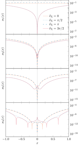
Fig. 6: Graphical demonstration of the validity of solution (36). It is evident that the residuals scale with the value of the resonance modification κ𝜅\kappa, and for each order n𝑛n of the solution, the remainder is of order 𝒪(κn+1)𝒪superscript𝜅𝑛1\mathcal{O}\!\left(\kappa^{n+1}\right).

Before we continue with our analysis, let us consider the asymptotic value of this solution in the limit of it’s validity, i.e. for 1|x|κ1much-less-than1𝑥much-less-thansuperscript𝜅11\ll|x|\ll\kappa^{-1}. The non-oscillating part of solution (36) can be written as

ω(x)x+f(κ).similar-to𝜔𝑥𝑥𝑓𝜅\displaystyle\omega(x)\sim x+f(\kappa). (37)

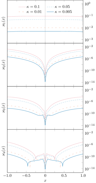
We see that any constant term in the solution for ω(x)𝜔𝑥\omega(x) is at least 𝒪(κ)𝒪𝜅\mathcal{O}\!\left(\kappa\right), rather than 𝒪(κ0)𝒪superscript𝜅0\mathcal{O}\!\left(\kappa^{0}\right). To confirm the validity of solution (36) we compute the quantities

ϰn+1=|ωnumω(n)(x)ωnum|,subscriptitalic-ϰ𝑛1subscript𝜔numsuperscript𝜔𝑛𝑥subscript𝜔num\displaystyle\varkappa_{n+1}=\left|\vphantom{\Bigg{[}\Bigg{]}}\frac{\omega_{\text{num}}-\omega^{(n)}(x)}{\omega_{\text{num}}}\right|, (38)

where ω(n)(x)superscript𝜔𝑛𝑥\omega^{(n)}(x) is eq. (36) restricted only to order n𝑛n (e.g. ω(1)(x)=ϖ0(x)+κϖ1(x)superscript𝜔1𝑥subscriptitalic-ϖ0𝑥𝜅subscriptitalic-ϖ1𝑥\omega^{(1)}(x)=\varpi_{0}(x)+\kappa\varpi_{1}(x)). If our solution is correct, then we would find that the fractional error, computed by the above formula is 𝒪(κn+1)𝒪superscript𝜅𝑛1\mathcal{O}\!\left(\kappa^{n+1}\right). This scaling is evident in the plot of these functions, shown in Figure 6.

Let us now seek a solution in the region of decaying oscillations, |x|1much-greater-than𝑥1|x|\gg 1. At lowest order, the solution is

ω0(x)=x.subscript𝜔0𝑥𝑥\displaystyle\omega_{0}(x)=x. (39)

At higher order, we attempt an ansatz, composed of a constant, a linear term, and a decaying oscillating term. We allow for three undetermined constants, a1,b1subscript𝑎1subscript𝑏1a_{1},b_{1} and c1subscript𝑐1c_{1}, as suggested by Gair, Yunes, and Bender (2012):

ω1(x)=a1+(1+b1)x+c1xsin[a1x+(1+b1)x2]subscript𝜔1𝑥subscript𝑎11subscript𝑏1𝑥subscript𝑐1𝑥subscript𝑎1𝑥1subscript𝑏1superscript𝑥2\displaystyle\omega_{1}(x)=a_{1}+\left(1+b_{1}\right)x+\frac{c_{1}}{x}\,\sin\!\Big{[}a_{1}x+\left(1+b_{1}\right)x^{2}\Big{]} (40)

where the subscript “1” on the slope correction term indicates that it pertains to the solution ω1(x)subscript𝜔1𝑥\omega_{1}(x), as the value of n𝑛n will change for higher-order solutions. When we substitute this ansatz into the model eq. (25):

ω1(x)1+κcos(xω1),similar-tosuperscriptsubscript𝜔1𝑥1𝜅𝑥subscript𝜔1\displaystyle\omega_{1}^{\prime}(x)\sim 1+\kappa\cos\left(x\omega_{1}\right), (41)

we ignore 𝒪(x1)𝒪superscript𝑥1\mathcal{O}\!\left(x^{-1}\right) terms and beyond, and use our knowledge of the behaviour of each separate term to reason about the values of the undetermined constants in eq. (42) below. Using standard trigonometric identities, we can expand the second term on the right-hand side, as shown explicitly in eq. (43) below.

1+b1+2(1+b1)c1cos[ax+(1+b1)x2]+𝒪(x1)1+κcos[ax+(1+b1)x2+c1sin[x+(1+b1)x2]]similar-to1subscript𝑏121subscript𝑏1subscript𝑐1𝑎𝑥1subscript𝑏1superscript𝑥2𝒪superscript𝑥11𝜅𝑎𝑥1subscript𝑏1superscript𝑥2subscript𝑐1𝑥1subscript𝑏1superscript𝑥2\displaystyle 1+b_{1}+2\left(1+b_{1}\right)c_{1}\cos\!\Big{[}ax+\left(1+b_{1}\right)x^{2}\Big{]}+\mathcal{O}\!\left(x^{-1}\right)\sim 1+\kappa\cos\!\left[ax+\left(1+b_{1}\right)x^{2}+c_{1}\sin\!\Big{[}x+(1+b_{1})x^{2}\Big{]}\vphantom{\Big{(}\Big{)}^{\!\!\!2\,}}\!\right] (42)
b1+2(1+b1)c1cos[ax+(1+b1)x2]+𝒪(x1)κcos[ax+(1+b1)x2]cos[c1sin[ax+(1+b1)x2]]κsin[ax+(1+b1)x2]sin[c1sin[ax+(1+b1)x2]]subscript𝑏1similar-to21subscript𝑏1subscript𝑐1𝑎𝑥1subscript𝑏1superscript𝑥2𝒪superscript𝑥1absentmissing-subexpressionsimilar-toabsent𝜅𝑎𝑥1subscript𝑏1superscript𝑥2subscript𝑐1𝑎𝑥1subscript𝑏1superscript𝑥2𝜅𝑎𝑥1subscript𝑏1superscript𝑥2subscript𝑐1𝑎𝑥1subscript𝑏1superscript𝑥2\displaystyle\quad\;\,\begin{aligned} b_{1}&+2\left(1+b_{1}\right)\,c_{1}\cos\!\Big{[}ax+\left(1+b_{1}\right)x^{2}\Big{]}+\mathcal{O}\!\left(x^{-1}\right)\sim\\ &\sim\kappa\cos\!\Big{[}ax+\left(1+b_{1}\right)x^{2}\Big{]}\cos\!\left[c_{1}\sin\!\Big{[}ax+\left(1+b_{1}\right)x^{2}\Big{]}\vphantom{\Big{(}\Big{)}^{\!\!\!2\,}}\!\right]-\kappa\sin\!\Big{[}ax+\left(1+b_{1}\right)x^{2}\Big{]}\sin\!\left[c_{1}\sin\!\Big{[}ax+\left(1+b_{1}\right)x^{2}\Big{]}\vphantom{\Big{(}\Big{)}^{\!\!\!2\,}}\!\right]\end{aligned} (43)

At this point we introduce a shorthand notation for the oscillating terms. Please refer to Appendix E (and the plots in Figure 26) for details.

Sn(x)sin[n(ax+(1+b)x2)]subscript𝑆𝑛𝑥𝑛𝑎𝑥1𝑏superscript𝑥2\displaystyle\,S_{n}(x)\equiv\sin\!\left[n\Big{(}ax+\left(1+b\right)x^{2}\Big{)}\vphantom{\Big{(}\Big{)}^{\!\!\!2\,}}\!\right] (44a)
Cn(x)cos[n(ax+(1+b)x2)]subscript𝐶𝑛𝑥𝑛𝑎𝑥1𝑏superscript𝑥2\displaystyle C_{n}(x)\equiv\cos\!\left[n\Big{(}ax+\left(1+b\right)x^{2}\Big{)}\vphantom{\Big{(}\Big{)}^{\!\!\!2\,}}\!\right] (44b)

Using these, we cast our last equation (43) in the form:

b1+2(1+b1)c1C1(x)+𝒪(x1)κC1(x)cos[c1S1(x)]κS1(x)sin[c1S1(x)]similar-tosubscript𝑏121subscript𝑏1subscript𝑐1subscript𝐶1𝑥𝒪superscript𝑥1𝜅subscript𝐶1𝑥subscript𝑐1subscript𝑆1𝑥𝜅subscript𝑆1𝑥subscript𝑐1subscript𝑆1𝑥\displaystyle\begin{split}b_{1}&+2\left(1+b_{1}\right)c_{1}C_{1}(x)+\mathcal{O}\!\left(x^{-1}\right)\sim\\ &\sim\kappa\,C_{1}(x)\cos\!\left[c_{1}S_{1}(x)\vphantom{()^{\!\!\!2\,}}\right]-\kappa\,S_{1}(x)\sin\!\left[c_{1}S_{1}(x)\vphantom{()^{\!\!\!2\,}}\right]\end{split} (45)

Comparing terms on both sides of eq. (45), we notice that in order for this identity to hold, it is necessary that c1𝒪(κ)similar-tosubscript𝑐1𝒪𝜅c_{1}\sim\mathcal{O}\!\left(\kappa\right). We remind ourselves of the assumption that κ1much-less-than𝜅1\kappa\ll 1 which justifies the small angle approximation we used above. Since the range of the sine function is between 11-1 and 1, and c1𝒪(κ)1similar-tosubscript𝑐1𝒪𝜅much-less-than1c_{1}\sim\mathcal{O}\!\left(\kappa\right)\ll 1, we can safely assume that c1sin[ax+(1+b)x2]1much-less-thansubscript𝑐1𝑎𝑥1𝑏superscript𝑥21c_{1}\sin\!\left[ax+\left(1+b\right)x^{2}\vphantom{()^{\!\!\!2\,}}\right]\ll 1 for all x𝑥x and expand both trigonometric terms in eq. (45):

b1+2(1+b1)c1C1(x)κC1(x)κc1S12(x)similar-tosubscript𝑏121subscript𝑏1subscript𝑐1subscript𝐶1𝑥𝜅subscript𝐶1𝑥𝜅subscript𝑐1superscriptsubscript𝑆12𝑥\displaystyle b_{1}+2\left(1+b_{1}\right)c_{1}C_{1}(x)\sim\kappa\,C_{1}(x)-\kappa\,c_{1}S_{1}^{2}(x) (46)

As we only retain the leading order terms in these expansions, we must disregard any 𝒪(κ3)𝒪superscript𝜅3\mathcal{O}\!\left(\kappa^{3}\right) or higher terms in our further calculations. Since we exclude them at this stage, such terms can no longer appear in the final solution for ω1(x)subscript𝜔1𝑥\omega_{1}(x). We match the coefficients of the two 𝒪(κ)𝒪𝜅\mathcal{O}\!\left(\kappa\right) terms on either side of the relation (46): 2(1+b)c1κsimilar-to21𝑏subscript𝑐1𝜅2\left(1+b\right)\,c_{1}\sim\kappa. Therefore:

c1κ2(1+b1).similar-tosubscript𝑐1𝜅21subscript𝑏1\displaystyle c_{1}\sim\frac{\kappa}{2\left(1+b_{1}\right)}. (47)

By using the double-angle trigonometric identities on the remaining term on the right-hand side of (46), we find

b1κc12(1C2(x))κc12.similar-tosubscript𝑏1𝜅subscript𝑐121subscript𝐶2𝑥similar-to𝜅subscript𝑐12\displaystyle b_{1}\!\sim-\frac{\kappa c_{1}}{2}\big{(}1-C_{2}(x)\big{)}\!\sim-\frac{\kappa c_{1}}{2}. (48)

Combining this with result (47), we establish that b1𝒪(κ2)similar-tosubscript𝑏1𝒪superscript𝜅2b_{1}\!\sim\mathcal{O}\!\left(\kappa^{2}\right), i.e., 0 to linear order. This result follows solely from the linear independence of the {Cn}subscript𝐶𝑛\{C_{n}\} terms. While they are not orthogonal (this can be easily verified by analytical integration), they are linearly independent, and therefore the coefficients on both sides need to match for eq. (48) to hold true. Similarly, we obtain the revised result c1κ/2+𝒪(κ3)similar-tosubscript𝑐1𝜅2𝒪superscript𝜅3c_{1}\sim\kappa/2+\mathcal{O}\!\left(\kappa^{3}\right). The additive constant aω(0)𝑎𝜔0a\equiv\omega(0) can be determined by comparing the limit |x|1much-greater-than𝑥1|x|\gg 1 of solution (36) to the ansatz (40) in the regime κ|x|1much-less-than𝜅𝑥1\kappa|x|\ll 1:

x±κ2π4+κ12sin(x2)x+𝒪(x2)a+x+κ12sin(x2)x+𝒪(κ3)similar-toplus-or-minus𝑥𝜅2𝜋4𝜅12superscript𝑥2𝑥𝒪superscript𝑥2𝑎𝑥𝜅12superscript𝑥2𝑥𝒪superscript𝜅3\displaystyle\begin{split}x\pm\kappa\,\frac{\sqrt{2\pi}}{4}&+\kappa\,\frac{1}{2}\,\frac{\sin\big{(}x^{2}\big{)}}{x}+\mathcal{O}\!\left(x^{-2}\right)\sim\\ &\sim a+x+\kappa\,\frac{1}{2}\,\frac{\sin\big{(}x^{2}\big{)}}{x}+\mathcal{O}\!\left(\kappa^{3}\right)\end{split} (49)

where on each side there are terms which we have ignored in the respective analysis. We find that a=±(2π/4)κ𝑎plus-or-minus2𝜋4𝜅a=\pm\big{(}\sqrt{2\pi}/4\big{)}\kappa to linear order, and we can write down the leading-order solution (50) to the frequency equation (for a single oscillatory mode and no initial phase). Note that here, and for the rest of this article, whenever the symbols ±/plus-or-minusminus-or-plus\nicefrac{{\pm}}{{\mp}} are used, the upper sign is valid for x0𝑥0x\geq 0, and the lower for x0𝑥0x\leq 0. The function in question is thus defined piecewise, but we will use this notation throughout for brevity.

ω1(x)=±2π4κ+x+κ121xsin(x2)subscript𝜔1𝑥plus-or-minus2𝜋4𝜅𝑥𝜅121𝑥superscript𝑥2\displaystyle\omega_{1}(x)=\pm\frac{\sqrt{2\pi}}{4}\,\kappa+x+\kappa\,\frac{1}{2}\,\frac{1}{x}\,\sin\!\big{(}x^{2}\big{)} (50)

Once we have established the suitability of this ansatz, we propose a further trial solution by adding an extra term to eq. (40). It accounts for the terms in eq. (48) we ignored when considering only first-order corrections:

c2xsin[2(ax+(1+b)x2)].subscript𝑐2𝑥2𝑎𝑥1𝑏superscript𝑥2\displaystyle\frac{c_{2}}{x}\,\sin\!\left[2\Big{(}ax+\left(1+b\right)x^{2}\Big{)}\vphantom{\Big{(}\Big{)}^{\!\!\!2\,}}\!\right]. (51)

The full ansatz can now be written as:

ω2(x)=a+(1+b2)x+c1xS1(x)+c2xS2(x).subscript𝜔2𝑥𝑎1subscript𝑏2𝑥subscript𝑐1𝑥subscript𝑆1𝑥subscript𝑐2𝑥subscript𝑆2𝑥\displaystyle\omega_{2}\left(x\right)=a+\left(1+b_{2}\right)x+\frac{c_{1}}{x}\,S_{1}(x)+\frac{c_{2}}{x}\,S_{2}(x). (52)

We substitute this into the source equation (25) and carry out a similar procedure to establish the new values of the constants, as detailed below. On the left-hand side, we ignore terms of 𝒪(x1)𝒪superscript𝑥1\mathcal{O}\!\left(x^{-1}\right) in the derivative:

ω21+b2+2(1+b2)c1C1+4(1+b2)c2C2,similar-tosuperscriptsubscript𝜔21subscript𝑏221subscript𝑏2subscript𝑐1subscript𝐶141subscript𝑏2subscript𝑐2subscript𝐶2\displaystyle\omega_{2}^{\prime}\sim 1+b_{2}+2\left(1+b_{2}\right)c_{1}\,C_{1}+4\left(1+b_{2}\right)c_{2}\,C_{2}\,, (53)

while on the right-hand side, we need to unpack the argument of the cosine function. Previously we established that c1𝒪(κ)similar-tosubscript𝑐1𝒪𝜅c_{1}\sim\mathcal{O}\!\left(\kappa\right), and since we expect that the new terms originating from ω2(x)subscript𝜔2𝑥\omega_{2}(x) will match the remaining term in eq. (48), we expect c2𝒪(κ2)similar-tosubscript𝑐2𝒪superscript𝜅2c_{2}\sim\mathcal{O}\!\left(\kappa^{2}\right). This justifies the further use of the small-angle approximation for the latter two terms. We point out that we need to ignore non-constant terms of 𝒪(κ3)𝒪superscript𝜅3\mathcal{O}\!\left(\kappa^{3}\right) in this expansion, as they will not be matched by a suitable term in the ansatz.

1+κcos[ax+(1+b2)x2+c1S1+c2S2]similar-to1𝜅𝑎𝑥1subscript𝑏2superscript𝑥2subscript𝑐1subscript𝑆1subscript𝑐2subscript𝑆2absent\displaystyle 1+\kappa\cos\!\left[ax+\left(1+b_{2}\right)x^{2}+c_{1}S_{1}+c_{2}S_{2}\vphantom{()^{\!\!\!2\,}}\right]\sim
1+κC1κc1S12κc2S1S2=similar-toabsent1𝜅subscript𝐶1𝜅subscript𝑐1superscriptsubscript𝑆12𝜅subscript𝑐2subscript𝑆1subscript𝑆2absent\displaystyle\quad\quad\sim 1+\kappa\,C_{1}-\kappa\,c_{1}S_{1}^{2}-\kappa\,c_{2}\,S_{1}S_{2}= (54)
=1κc12+κC1(x)κc12C2(x)+𝒪(κ3)absent1𝜅subscript𝑐12𝜅subscript𝐶1𝑥𝜅subscript𝑐12subscript𝐶2𝑥𝒪superscript𝜅3\displaystyle\quad\quad\quad\quad=1-\frac{\kappa c_{1}}{2}+\kappa\,C_{1}(x)-\frac{\kappa c_{1}}{2}\,C_{2}(x)+\mathcal{O}\!\left(\kappa^{3}\right)

Matching the coefficients of terms in eqs. (53) and (54), we obtain the coupled equations:

b2κc12,2(1+b2)c1κ,4(1+b2)c2κc12.formulae-sequencesimilar-tosubscript𝑏2𝜅subscript𝑐12formulae-sequencesimilar-to21subscript𝑏2subscript𝑐1𝜅similar-to41subscript𝑏2subscript𝑐2𝜅subscript𝑐12\displaystyle b_{2}\!\sim-\frac{\kappa c_{1}}{2},~{}2\left(1+b_{2}\right)c_{1}\sim\kappa,~{}4\left(1+b_{2}\right)c_{2}\sim\frac{\kappa c_{1}}{2}. (55)

These imply that c1κ/2+𝒪(κ3)similar-tosubscript𝑐1𝜅2𝒪superscript𝜅3c_{1}\sim\kappa/2+\mathcal{O}\!\left(\kappa^{3}\right) and b2κ2/4+𝒪(κ4)similar-tosubscript𝑏2superscript𝜅24𝒪superscript𝜅4b_{2}\!\sim-\kappa^{2}/4+\mathcal{O}\!\left(\kappa^{4}\right). The last equation above determines the value of the newly introduced constant c2subscript𝑐2c_{2}:

c2κc18(1+b2)κ216(1+b2)κ216+𝒪(κ4).similar-tosubscript𝑐2𝜅subscript𝑐181subscript𝑏2similar-tosuperscript𝜅2161subscript𝑏2similar-tosuperscript𝜅216𝒪superscript𝜅4\displaystyle c_{2}\sim\frac{\kappa c_{1}}{8\left(1+b_{2}\right)}\sim\frac{\kappa^{2}}{16\left(1+b_{2}\right)}\sim\frac{\kappa^{2}}{16}+\mathcal{O}\!\left(\kappa^{4}\right). (56)

To find the constant a𝑎a at second order, we need to match this solution to the 𝒪(κ2)𝒪superscript𝜅2\mathcal{O}\!\left(\kappa^{2}\right) part of solution (36) in the buffer zone where both solutions are valid, as per eq. (57). Expanding (36) for x1much-greater-than𝑥1x\gg 1 and the above ansatz for κ|x|1much-less-than𝜅𝑥1\kappa|x|\ll 1 (both to order 𝒪(x1)𝒪superscript𝑥1\mathcal{O}\!\left(x^{-1}\right) inclusive), we find that all functional term match on both sides. The constant term is the value of a𝑎a at second order, (π/16)κ2minus-or-plus𝜋16superscript𝜅2\big{(}\!\mp\sqrt{\pi}/16\big{)}\kappa^{2}.

Combining these results together, we establish the improved solution ω2(x)subscript𝜔2𝑥\omega_{2}(x), given by eq. (58).

2π4cos(x2)C(2xπ)π8C(4xπ)14x|x1=a14x+2π8cos(x2)+116sin(2x2)x2+𝒪(x2)2𝜋4superscript𝑥2𝐶2𝑥𝜋𝜋8𝐶4𝑥𝜋evaluated-at14𝑥much-greater-than𝑥1𝑎14𝑥2𝜋8superscript𝑥21162superscript𝑥2superscript𝑥2𝒪superscript𝑥2\displaystyle\left.\frac{\sqrt{2\pi}}{4}\,\cos\!\big{(}x^{2}\big{)}\,C\!\left(\!\frac{\sqrt{2}\,x}{\sqrt{\pi}}\!\right)\!-\frac{\sqrt{\pi}}{8}\,C\!\left(\!\frac{\sqrt{4}\,x}{\sqrt{\pi}}\!\right)\!-\frac{1}{4}\,x\,\right|_{x\gg 1}\!\!=a-\frac{1}{4}\,x+\frac{\sqrt{2\pi}}{8}\,\cos\!\big{(}x^{2}\big{)}+\frac{1}{16}\,\frac{\sin\!\big{(}2x^{2}\big{)}}{x^{2}}+\mathcal{O}\!\left(x^{-2}\right) (57)
ω2(x)=±2π4κπ16κ2+(1κ24)x+κ121xsin[(±2π4κ)x+x2]+κ21161xsin(2x2)subscript𝜔2𝑥minus-or-plusplus-or-minus2𝜋4𝜅𝜋16superscript𝜅21superscript𝜅24𝑥𝜅121𝑥plus-or-minus2𝜋4𝜅𝑥superscript𝑥2superscript𝜅21161𝑥2superscript𝑥2\displaystyle\omega_{2}(x)=\pm\,\frac{\sqrt{2\pi}}{4}\,\kappa\mp\frac{\sqrt{\pi}}{16}\,\kappa^{2}+\!\Bigg{(}\!1-\frac{\kappa^{2}}{4}\!\Bigg{)}x+\kappa\,\frac{1}{2}\,\frac{1}{x}\,\sin\!\left[\!\vphantom{\Bigg{[}\Bigg{]}^{\!\!\!2\,}}\left(\!\pm\,\frac{\sqrt{2\pi}}{4}\,\kappa\!\right)\!x+x^{2}\right]\!+\kappa^{2}\,\frac{1}{16}\,\frac{1}{x}\,\sin\!\left(2x^{2}\right) (58)

At the next order, the task of finding appropriate terms becomes more complicated, since we need to balance the terms in eq. (34). At this order there is a logarithmic trend, as well as an oscillatory part, hence we propose the following ansatz which reflects the nature of the solution:

ω3(x)=asubscript𝜔3𝑥𝑎\displaystyle\omega_{3}(x)=a +(1+b3)x+c1S1(x)x+c2S2(x)x+c3S3(x)x1subscript𝑏3𝑥subscript𝑐1subscript𝑆1𝑥𝑥subscript𝑐2subscript𝑆2𝑥𝑥subscript𝑐3subscript𝑆3𝑥𝑥\displaystyle+\left(1+b_{3}\right)x+c_{1}\frac{S_{1}(x)}{x}+c_{2}\frac{S_{2}(x)}{x}+c_{3}\frac{S_{3}(x)}{x}
+d1S1(x)x2+d2S2(x)x2+lln|x|.subscript𝑑1subscript𝑆1𝑥superscript𝑥2subscript𝑑2subscript𝑆2𝑥superscript𝑥2𝑙𝑥\displaystyle+d_{1}\frac{S_{1}(x)}{x^{2}}+d_{2}\frac{S_{2}(x)}{x^{2}}+l\ln\!|x|. (59)

The details of calculating the expressions for these constants are burdensome, hence we have left them in Appendix I. The important message here is that we have still managed to find a set of terms which satisfy the governing equation (25), without conflicting the previous solutions (i.e. without producing new terms at 𝒪(κ,x1)𝒪𝜅superscript𝑥1\mathcal{O}\!\left(\kappa,x^{-1}\right)).

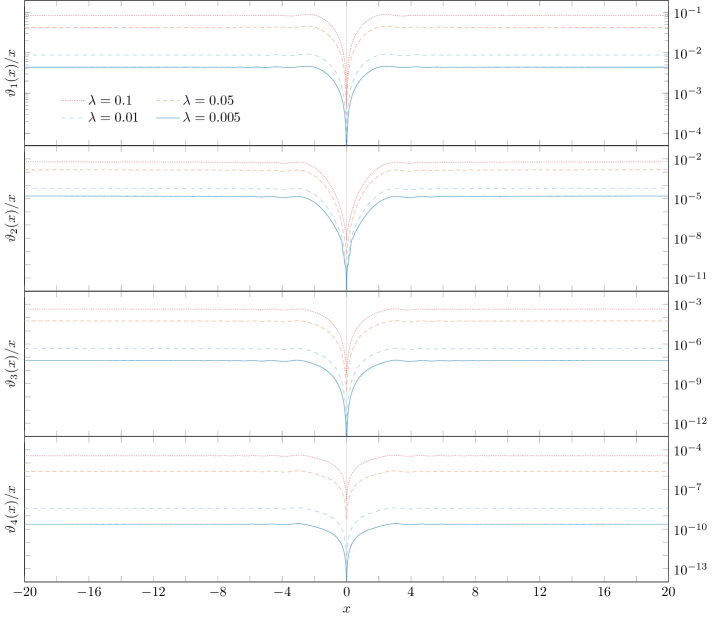
Refer to caption
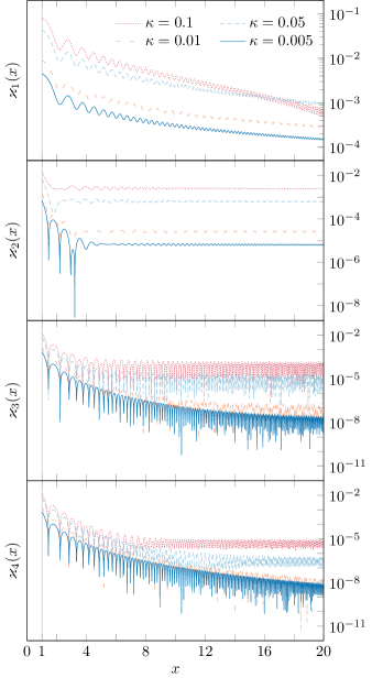
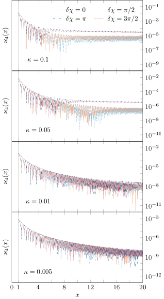
Fig. 7: Graphical demonstration of the validity of solutions (39) – (64). The fractional errors scale with the value of the resonance modification κ𝜅\kappa. At each order n𝑛n of the solution, the remainder is of order 𝒪(κn+1)𝒪superscript𝜅𝑛1\mathcal{O}\!\left(\kappa^{n+1}\right), as expected.

To determine the new value of the constant a𝑎a, we again need to turn to our solution near the origin. In particular, here we need an expansion of ϖ3(x)subscriptitalic-ϖ3𝑥\varpi_{3}(x) for large x𝑥x. However, we used a small-x𝑥x approximation to obtain ϖ3aasymp(x)subscriptitalic-ϖ3subscript𝑎asymp𝑥\varpi_{3a_{\rm asymp}}(x) earlier, which is not valid in the buffer zone where both solutions (36) and (59) are valid. We need to go back to the original problem (32a), and instead of expanding in the small-x𝑥x regime, we expand for |x|1much-greater-than𝑥1|x|\gg 1 (which is valid when κ|x|1much-less-than𝜅𝑥1\kappa|x|\ll 1). To do this, we expand the Fresnel term on the right hand side of eq. (32a) for large |x|𝑥|x|, truncate the series at 𝒪(x5)𝒪superscript𝑥5\mathcal{O}\!\left(x^{-5}\right) and then compute the antiderivative of this series, the function ϖ3aasympsubscriptitalic-ϖ3subscript𝑎asymp\varpi_{3a_{\rm asymp}} given in eq. (62). This procedure ensures that ϖ3a(x)ϖ3aasymp(x)α+𝒪(x4)similar-tosubscriptitalic-ϖ3𝑎𝑥subscriptitalic-ϖ3subscript𝑎asymp𝑥𝛼𝒪superscript𝑥4\varpi_{3a}(x)-\varpi_{3a_{\rm asymp}}(x)\sim\alpha+\mathcal{O}\!\left(x^{-4}\right). The constant α𝛼\alpha is the asymptotic value of ϖ3a(x)ϖ3aasymp(x)subscriptitalic-ϖ3𝑎𝑥subscriptitalic-ϖ3subscript𝑎asymp𝑥\varpi_{3a}(x)-\varpi_{3a_{\rm asymp}}(x), which may be found by integrating ϖ3a(x)ϖ3aasymp(x)subscriptitalic-ϖ3𝑎𝑥subscriptitalic-ϖ3subscript𝑎asymp𝑥\varpi_{3a}(x)-\varpi_{3a_{\rm asymp}}(x) from 00 to infinity

α=0xcdyϖ3a(y)ϖ3aasymp(xc)+xcdy(ϖ3a(y)ϖ3aasymp(y)).𝛼superscriptsubscript0subscript𝑥𝑐differential-d𝑦superscriptsubscriptitalic-ϖ3𝑎𝑦subscriptitalic-ϖ3subscript𝑎asympsubscript𝑥𝑐superscriptsubscriptsubscript𝑥𝑐differential-d𝑦superscriptsubscriptitalic-ϖ3𝑎𝑦superscriptsubscriptitalic-ϖ3subscript𝑎asymp𝑦\displaystyle\begin{split}\alpha=&\int_{0}^{x_{c}}\!\!\!\!\mathop{}\!\mathrm{d}y\,\varpi_{3a}^{\prime}(y)-\varpi_{3a_{\rm asymp}}(x_{c})\\ &\quad\quad+\!\int_{x_{c}}^{\infty}\!\!\!\!\mathop{}\!\mathrm{d}y\,\big{(}\varpi_{3a}^{\prime}(y)-\varpi_{3a_{\rm asymp}}^{\prime}(y)\big{)}.\end{split} (60)

The quantity xcsubscript𝑥𝑐x_{c} is arbitrary, but by choosing a value xc1/k010similar-tosubscript𝑥𝑐1subscript𝑘0similar-to10x_{c}\sim 1/k_{0}\sim 10 we may bound the value of the second integral by 105superscript10510^{-5}. Numerical evaluation of the terms on the first line of eq. (60) then give α= 0.00991𝛼minus-or-plus0.00991\alpha=\mp\,0.00991. We deduce that, asymptotically, we may write ϖ3(x)=α+ϖ3aasymp(x)+ϖ3b(x)subscriptitalic-ϖ3𝑥𝛼subscriptitalic-ϖ3subscript𝑎asymp𝑥subscriptitalic-ϖ3𝑏𝑥\varpi_{3}(x)=\alpha+\varpi_{3a_{\rm asymp}}(x)+\varpi_{3b}(x), with higher-order corrections which scale as x4superscript𝑥4x^{-4}.

Combining these resulting terms with the ones coming from eq. (35), we arrive at the left-hand side of eq. (63). The right-hand side of eq. (63) is comprised of the terms in an expansion of the ansatz (59) for small κ|x|𝜅𝑥\kappa|x|.

The terms match nicely as we would expect, apart from the coefficients of sin(x2)/xsuperscript𝑥2𝑥\sin\!\big{(}x^{2}\big{)}/x and cos(x2)/xsuperscript𝑥2𝑥\cos\!\big{(}x^{2}\big{)}/x. The reason for this is that to determine these terms accurately we need to extend the asymptotic solution to the next order in 1/x1𝑥1/x. At that order we get a term of the form C1(x)/x3subscript𝐶1𝑥superscript𝑥3C_{1}(x)/x^{3} in the solution, and it is straightforward to deduce that, at leading order, the coefficient in front of this term is κ/4𝜅4-\,\kappa/4. This additional term contributes terms at order κ3superscript𝜅3\kappa^{3} on the right hand side of eq. (63) and those terms are πcos(x2)/(64x)𝜋superscript𝑥264𝑥\pi\cos\!\big{(}x^{2}\big{)}/(64x) and sin(x2)/(16x)superscript𝑥216𝑥-\sin\!\big{(}x^{2}\big{)}/(16x), which are exactly what is needed to match the terms from the κ|x|1much-less-than𝜅𝑥1\kappa|x|\ll 1 solution on the left hand side of eq. (63).

We can now read off the third-order piece of the coefficient a𝑎a from eq. (63)

a3=(α±2π32±6π192±2π3/2128)κ3± 0.15255κ3subscript𝑎3plus-or-minus𝛼2𝜋326𝜋1922superscript𝜋32128superscript𝜅3plus-or-minus0.15255superscript𝜅3\displaystyle a_{3}=\left(\!\alpha\pm\frac{\sqrt{2\pi}}{32}\pm\frac{\sqrt{6\pi}}{192}\pm\frac{\sqrt{2}\,\pi^{\nicefrac{{3}}{{2}}}}{128}\!\right)\!\kappa^{3}\approx\pm\,0.15255\,\kappa^{3} (61)

The third-order solution ω3(x)subscript𝜔3𝑥\omega_{3}(x) is given in eq. (64). This is the most accurate solution to the single-mode, zero-phase frequency equation that we will present. The lack of necessity for higher order iterations will be explained when discussing the multi-mode frequency equation.

Once we have obtained these solutions, it is worthwhile to investigate their properties visually. To confirm their validity, Figure 7 demonstrates that these solutions are correct at their respective order by computing the quantities ϰn(x)subscriptitalic-ϰ𝑛𝑥\varkappa_{n}(x) defined in eq. (38), and showing graphically that they have the expected magnitudes. Please note we have shown only the region x>0𝑥0x>0, with the region x<0𝑥0x<0 being a mirror image of this one.

Figure 8 shows how the intercept a𝑎a, the slope (1b)1𝑏(1-b), and the coefficients of the oscillating modes {cn}subscript𝑐𝑛\{c_{n}\} and {dn}subscript𝑑𝑛\{d_{n}\} vary with the parameter κ𝜅\kappa.

ϖ3aasymp(x)=subscriptitalic-ϖ3subscript𝑎asymp𝑥absent\displaystyle\varpi_{3a_{\rm asymp}}(x)= ±2π32ln|x|2π64C(2xπ)+2π3/264S(2xπ)+6π192C(6xπ)π32xsin(x2)±2π64cos(2x2)plus-or-minusplus-or-minus2𝜋32𝑥2𝜋64𝐶2𝑥𝜋2superscript𝜋3264𝑆2𝑥𝜋6𝜋192𝐶6𝑥𝜋𝜋32𝑥superscript𝑥22𝜋642superscript𝑥2\displaystyle\pm\frac{\sqrt{2\pi}}{32}\,\ln\!|x|-\frac{\sqrt{2\pi}}{64}\,C\!\left(\!\frac{\sqrt{2}\,x}{\sqrt{\pi}}\!\right)\!+\frac{\sqrt{2}\,\pi^{\nicefrac{{3}}{{2}}}}{64}\,S\!\left(\!\frac{\sqrt{2}\,x}{\sqrt{\pi}}\!\right)\!+\frac{\sqrt{6\pi}}{192}\,C\!\left(\!\frac{\sqrt{6}\,x}{\sqrt{\pi}}\!\right)\!-\frac{\pi}{32}\,x\sin\!\big{(}x^{2}\big{)}\pm\frac{\sqrt{2\pi}}{64}\,\cos\!\big{(}2x^{2}\big{)}
±2π128sin(2x2)x2164cos(x2)x31192cos(3x2)x32π64cos(2x2)x43256sin(x2)x53256sin(3x2)x5minus-or-plusplus-or-minus2𝜋1282superscript𝑥2superscript𝑥2164superscript𝑥2superscript𝑥311923superscript𝑥2superscript𝑥32𝜋642superscript𝑥2superscript𝑥43256superscript𝑥2superscript𝑥532563superscript𝑥2superscript𝑥5\displaystyle\pm\frac{\sqrt{2\pi}}{128}\,\frac{\sin\!\big{(}2x^{2}\big{)}}{x^{2}}-\frac{1}{64}\,\frac{\cos\!\big{(}x^{2}\big{)}}{x^{3}}-\frac{1}{192}\,\frac{\cos\!\big{(}3x^{2}\big{)}}{x^{3}}\mp\frac{\sqrt{2\pi}}{64}\,\frac{\cos\!\big{(}2x^{2}\big{)}}{x^{4}}-\frac{3}{256}\,\frac{\sin\!\big{(}x^{2}\big{)}}{x^{5}}-\frac{3}{256}\,\frac{\sin\!\big{(}3x^{2}\big{)}}{x^{5}} (62)
α±2π32±6π192±2π3/2128±2π32ln|x|π32xsin(x2)plus-or-minus𝛼2𝜋326𝜋1922superscript𝜋321282𝜋32𝑥𝜋32𝑥superscript𝑥2\displaystyle\alpha\pm\frac{\sqrt{2\pi}}{32}\pm\frac{\sqrt{6\pi}}{192}\pm\frac{\sqrt{2}\,\pi^{\nicefrac{{3}}{{2}}}}{128}\pm\frac{\sqrt{2\pi}}{32}\,\ln\!|x|-\frac{\pi}{32}\,x\,\sin\!\left(x^{2}\right) 18xcos(x2)π32cos(x2)±2π32cos(2x2)plus-or-minusminus-or-plus18𝑥superscript𝑥2𝜋32superscript𝑥22𝜋322superscript𝑥2\displaystyle-\frac{1}{8}\,x\,\cos\!\left(x^{2}\right)\mp\frac{\sqrt{\pi}}{32}\,\cos\!\left(x^{2}\right)\pm\frac{\sqrt{2\pi}}{32}\,\cos\!\left(2x^{2}\right) +132sin(x2)x+196sin(3x2)xπ64cos(x2)x132superscript𝑥2𝑥1963superscript𝑥2𝑥𝜋64superscript𝑥2𝑥\displaystyle+\frac{1}{32}\,\frac{\sin\!\left(x^{2}\right)}{x}+\frac{1}{96}\,\frac{\sin\!\left(3x^{2}\right)}{x}-\frac{\pi}{64}\,\frac{\cos\!\left(x^{2}\right)}{x} =\quad= a3π32xsin(x2)π32cos(x2)18xcos(x2)minus-or-plussubscript𝑎3𝜋32𝑥superscript𝑥2𝜋32superscript𝑥218𝑥superscript𝑥2\displaystyle a_{3}\mp\frac{\pi}{32}\,x\,\sin\!\left(x^{2}\right)\mp\frac{\sqrt{\pi}}{32}\,\cos\!\left(x^{2}\right)-\frac{1}{8}\,x\,\cos\!\left(x^{2}\right) ±2π32cos(2x2)+332sin(x2)x+196sin(3x2)xplus-or-minus2𝜋322superscript𝑥2332superscript𝑥2𝑥1963superscript𝑥2𝑥\displaystyle\pm\frac{\sqrt{2\pi}}{32}\,\cos\!\left(2x^{2}\right)+\frac{3}{32}\,\frac{\sin\!\left(x^{2}\right)}{x}+\frac{1}{96}\,\frac{\sin\!\left(3x^{2}\right)}{x} π32cos(x2)x±2π32ln|x|plus-or-minus𝜋32superscript𝑥2𝑥2𝜋32𝑥\displaystyle-\frac{\pi}{32}\,\frac{\cos\!\left(x^{2}\right)}{x}\pm\frac{\sqrt{2\pi}}{32}\,\ln\!|x| (63)
ω3(x)=±(2π4κπ16κ2+0.15255κ3)+(1κ24)x+κ121xsin[(±2π4κπ16κ2)x+(1κ24)x2]subscript𝜔3𝑥plus-or-minus2𝜋4𝜅𝜋16superscript𝜅20.15255superscript𝜅31superscript𝜅24𝑥𝜅121𝑥minus-or-plusplus-or-minus2𝜋4𝜅𝜋16superscript𝜅2𝑥1superscript𝜅24superscript𝑥2\displaystyle\omega_{3}(x)=\pm\left(\!\frac{\sqrt{2\pi}}{4}\,\kappa-\frac{\sqrt{\pi}}{16}\,\kappa^{2}+0.15255\,\kappa^{3}\!\right)\!+\!\left(\!\vphantom{\Bigg{[}\Bigg{]}}1-\frac{\kappa^{2}}{4}\!\right)\!x+\kappa\,\frac{1}{2}\,\frac{1}{x}\,\sin\!\left[\vphantom{\Bigg{[}\Bigg{]}^{\!\!\!2\,}}\!\left(\!\pm\frac{\sqrt{2\pi}}{4}\,\kappa\mp\frac{\sqrt{\pi}}{16}\,\kappa^{2}\!\right)\!x+\!\Bigg{(}\!1-\frac{\kappa^{2}}{4}\!\Bigg{)}x^{2}\right]
+κ21161xsin[2((±2π4κ)x+x2)]+κ31x(332sin(x2)+196sin(3x2))superscript𝜅21161𝑥2plus-or-minus2𝜋4𝜅𝑥superscript𝑥2superscript𝜅31𝑥332superscript𝑥21963superscript𝑥2\displaystyle\quad\quad\quad\quad+\kappa^{2}\frac{1}{16}\,\frac{1}{x}\,\sin\!\left[\vphantom{\left[\Bigg{[}\Bigg{]}^{\!\!\!2\,}\right]^{\!\!\!2\,}}2\!\left(\!\!\vphantom{\Bigg{[}\Bigg{]}^{\!\!\!2\,}}\left(\!\pm\,\frac{\sqrt{2\pi}}{4}\,\kappa\!\right)\!x+x^{2}\!\right)\!\right]\!+\kappa^{3}\,\frac{1}{x}\!\left(\!\vphantom{\Bigg{[}\Bigg{]}}\frac{3}{32}\,\sin\!\left(x^{2}\right)+\frac{1}{96}\,\sin\!\left(3x^{2}\right)\!\right) (64)
κ22π161x2sin[(±2π4κ)x+x2]±κ3(π641x2sin(x2)2π641x2sin(2x2)+2π32ln|x|)plus-or-minusminus-or-plussuperscript𝜅22𝜋161superscript𝑥2plus-or-minus2𝜋4𝜅𝑥superscript𝑥2superscript𝜅3𝜋641superscript𝑥2superscript𝑥22𝜋641superscript𝑥22superscript𝑥22𝜋32𝑥\displaystyle\quad\quad\quad\quad\quad\quad\quad\quad\mp\kappa^{2}\frac{\sqrt{2\pi}}{16}\,\frac{1}{x^{2}}\,\sin\!\left[\vphantom{\Bigg{[}\Bigg{]}^{\!\!\!2\,}}\!\!\vphantom{\Bigg{[}\Bigg{]}^{\!\!\!2\,}}\left(\!\pm\,\frac{\sqrt{2\pi}}{4}\,\kappa\!\right)\!x+x^{2}\right]\!\pm\kappa^{3}\!\left(\!\vphantom{\Bigg{[}\Bigg{]}}\frac{\sqrt{\pi}}{64}\,\frac{1}{x^{2}}\,\sin\!\left(x^{2}\right)-\frac{\sqrt{2\pi}}{64}\,\frac{1}{x^{2}}\,\sin\!\left(2x^{2}\right)+\frac{\sqrt{2\pi}}{32}\,\ln\!|x|\!\right)
[Uncaptioned image]
Table 1: The first 10 terms of the series {kn}subscript𝑘𝑛\{k_{n}\} for the three different series of interest, for each of our 4 chosen numerical values: 0.1,0.05,0.010.10.050.010.1,0.05,0.01, and 0.0050.0050.005. These were plotted in Figure 2. It should be noted that the numbers in this table are given using the scientific notation a.bc¯da.bc¯×10dsuperscript¯formulae-sequence𝑎𝑏𝑐𝑑¯formulae-sequence𝑎𝑏𝑐superscript10𝑑\overline{a.bc}^{\,d}\equiv\overline{a.bc}\times\!10^{d}. The horizontal lines in the data represent numerical boundaries: numbers below the first line in a column are smaller than ki2superscriptsubscript𝑘𝑖2k_{i}^{2}, and numbers below the second line are smaller than ki3superscriptsubscript𝑘𝑖3k_{i}^{3}.

The solution can be made more accurate, by adding terms at higher orders, of the form cnSn(x)/xsubscript𝑐𝑛subscript𝑆𝑛𝑥𝑥c_{n}S_{n}(x)/x and djSn(x)/x2subscript𝑑𝑗subscript𝑆𝑛𝑥superscript𝑥2d_{j}S_{n}(x)/x^{2} to the ansatz (52). Below we see the general case of having m𝑚m oscillatory terms in the trial solution ωm(x)subscript𝜔𝑚𝑥\omega_{m}(x), where m𝑚m could be either a finite number or infinity:

ωm(x)=a+(1+b)x+j=1m(cjSj(x)x+djSj(x)x2).subscript𝜔𝑚𝑥𝑎1𝑏𝑥superscriptsubscript𝑗1𝑚subscript𝑐𝑗subscript𝑆𝑗𝑥𝑥subscript𝑑𝑗subscript𝑆𝑗𝑥superscript𝑥2\displaystyle\omega_{m}(x)=a+\left(1+b\right)x+\sum_{j=1}^{m}\left(c_{j}\frac{S_{j}(x)}{x}+d_{j}\frac{S_{j}(x)}{x^{2}}\right). (65)

We shall discuss later (after we solve the multimode version of the phase equation) why there is no practical need for solutions beyond third order. If we seek to find lower-order corrections in 𝒪(xp)𝒪superscript𝑥𝑝\mathcal{O}\!\left(x^{-p}\right), we add terms of the form:

1xpj=1m(cj(p)Sj(x)+dj(p)Cj(x)).similar-toabsent1superscript𝑥𝑝superscriptsubscript𝑗1𝑚superscriptsubscript𝑐𝑗𝑝subscript𝑆𝑗𝑥superscriptsubscript𝑑𝑗𝑝subscript𝐶𝑗𝑥\displaystyle\sim\frac{1}{x^{p}}\sum_{j=1}^{m}\left(c_{j}^{(p)}S_{j}(x)+d_{j}^{(p)}C_{j}(x)\right). (66)

However, instead of following through with this procedure, we look at extensions of eq. (25) to find the general solution of eq. (19a). Initially, we allow for multiple oscillation modes, each with a different amplitude (parameter κisubscript𝜅𝑖\kappa_{i}), and following this, we include a non-vanishing phase in our calculations.

In the following we will use bold quantities, e.g., 𝝎(x)𝝎𝑥\bm{\omega}(x), to indicate values of the coefficients in the multiple mode case. We note that these are not vectors, but the scalars that appear in the multiple mode solution. To solve for the evolution of the frequency resonances,

𝝎(x)=1+nκncos(nxω𝝎)superscript𝝎𝑥1subscript𝑛subscript𝜅𝑛𝑛subscript𝑥𝜔𝝎\displaystyle\bm{\omega}^{\prime}(x)=1+\sum_{n}\kappa_{n}\cos\left(nx_{\omega}\,\bm{\omega}\right) (67)

we can again look at the problem from two scales: small and large |x|𝑥|x|. Near the origin, we can write down a series expansion similar to eq. (26):

𝝎(x)=m=0n=0κnmϖm,n(x).𝝎𝑥superscriptsubscript𝑚0superscriptsubscript𝑛0superscriptsubscript𝜅𝑛𝑚subscriptbold-italic-ϖ𝑚𝑛𝑥\displaystyle\bm{\omega}(x)=\sum_{m=0}^{\infty}\sum_{n=0}^{\infty}\,\kappa_{n}^{m}\bm{\varpi}_{m,n}(x). (68)

Similarly to before, we can derive solutions for n=0,1𝑛01n=0,1:

ϖ0,n(x)subscriptbold-italic-ϖ0𝑛𝑥\displaystyle\bm{\varpi}_{0,n}(x) =xabsent𝑥\displaystyle=x (69a)
ϖ1,n(x)subscriptbold-italic-ϖ1𝑛𝑥\displaystyle\bm{\varpi}_{1,n}(x) =π2nC(2nxπ)absent𝜋2𝑛𝐶2𝑛𝑥𝜋\displaystyle=\frac{\sqrt{\pi}}{\sqrt{2n}}\,C\!\left(\!\frac{\sqrt{2n}\,x}{\sqrt{\pi}}\!\right) (69b)

Further solutions are not going to be pursued, as higher orders of κnsubscript𝜅𝑛\kappa_{n} (for small n𝑛n) would be of the same size as κnsubscript𝜅𝑛\kappa_{n} for some larger n𝑛n. Hence, 𝝎(x)𝝎𝑥\bm{\omega}(x) near the origin can be most completely written down as

𝝎(x)=x+nκnπ2nC(2nxπ)𝝎𝑥𝑥subscript𝑛subscript𝜅𝑛𝜋2𝑛𝐶2𝑛𝑥𝜋\displaystyle\bm{\omega}(x)=x+\sum_{n}\kappa_{n}\frac{\sqrt{\pi}}{\sqrt{2n}}\,C\!\left(\!\frac{\sqrt{2n}\,x}{\sqrt{\pi}}\!\right) (70)

For |x|1much-greater-than𝑥1|x|\gg 1, we propose an extended ansatz of the form:

𝝎1(x)=𝒂+(1+𝒃1)x+n𝒄nSn(x)xsubscript𝝎1𝑥𝒂1subscript𝒃1𝑥subscript𝑛subscript𝒄𝑛subscript𝑆𝑛𝑥𝑥\displaystyle\bm{\omega}_{1}(x)=\bm{a}+\left(1+\bm{b}_{1}\right)x+\sum_{n}\bm{c}_{n}\,\frac{S_{n}(x)}{x} (71)

with derivative

𝝎1=1+𝒃1+n2n(1+𝒃)𝒄nCn(x)+𝒪(x1).superscriptsubscript𝝎11subscript𝒃1subscript𝑛2𝑛1𝒃subscript𝒄𝑛subscript𝐶𝑛𝑥𝒪superscript𝑥1\displaystyle\bm{\omega}_{1}^{\prime}=1+\bm{b}_{1}+\sum_{n}2n\!\left(1+\bm{b}\right)\bm{c}_{n}C_{n}(x)+\mathcal{O}\!\left(x^{-1}\right). (72)

We substitute this into the governing eq. (67) and proceed to match the relevant coefficients on both sides of this relation. It is important to explain here that the leading order dependence of each coefficient 𝒄nsubscript𝒄𝑛\bm{c}_{n} will be the same as if considering its corresponding mode on its own (see Appendix II for derivation), with higher-order corrections due to cross-terms emerging from the cosine term (see Appendix III), and therefore 𝒄n𝒪(κn/n)𝒪(κ1/nα+1)similar-tosubscript𝒄𝑛𝒪subscript𝜅𝑛𝑛similar-to𝒪subscript𝜅1superscript𝑛𝛼1\bm{c}_{n}\sim\mathcal{O}\!\left(\kappa_{n}/n\right)\sim\mathcal{O}\!\left(\kappa_{1}/n^{\alpha+1}\right). Thus, each coefficient 𝒄nsubscript𝒄𝑛\bm{c}_{n} is smaller than the previous one in the series, and we can expand the trigonometric terms on the right-hand side, to obtain the form (73). Evidently, to be able to match the constant term 𝒃𝒃\bm{b} on the left-hand side, we need to find a constant term on the right-hand side too. Such a constant could only arise from the second term on the right-hand side, in the case n=m𝑛𝑚n=m, and yields eq. (74). The remaining terms must combine to form an expression for 𝒄nsubscript𝒄𝑛\bm{c}_{n}, and we match them using the linear independency of the functions {Cn(x)}subscript𝐶𝑛𝑥\{C_{n}(x)\}, yielding eq. (75). On the right-hand side of this equation, we omitted a pre-factor of (1+𝒃)11+𝒪(κ12)similar-tosuperscript1𝒃11𝒪superscriptsubscript𝜅12(1+\bm{b})^{-1}\sim 1+\mathcal{O}\!\left(\kappa_{1}^{2}\right), since we know that 𝒃𝒪(κ12)similar-to𝒃𝒪superscriptsubscript𝜅12\bm{b}\sim\mathcal{O}\!\left(\kappa_{1}^{2}\right). 𝒃+2(1+𝒃)nn𝒄nCn(x)nκnCn(x)12n,mnκn𝒄mCnm(x)+12n,mnκn𝒄mCn+m(x)similar-to𝒃21𝒃subscript𝑛𝑛subscript𝒄𝑛subscript𝐶𝑛𝑥subscript𝑛subscript𝜅𝑛subscript𝐶𝑛𝑥12subscript𝑛𝑚𝑛subscript𝜅𝑛subscript𝒄𝑚subscript𝐶𝑛𝑚𝑥12subscript𝑛𝑚𝑛subscript𝜅𝑛subscript𝒄𝑚subscript𝐶𝑛𝑚𝑥\displaystyle\bm{b}+2(1+\bm{b})\sum_{n}n\,\bm{c}_{n}C_{n}(x)\sim\sum_{n}\kappa_{n}\,C_{n}(x)-\frac{1}{2}\sum_{n,\,m}n\,\kappa_{n}\,\bm{c}_{m}C_{n-m}(x)+\frac{1}{2}\sum_{n,\,m}n\,\kappa_{n}\,\bm{c}_{m}C_{n+m}(x) (73)
𝒃12nnκn𝒄nsimilar-to𝒃12subscript𝑛𝑛subscript𝜅𝑛subscript𝒄𝑛\displaystyle\bm{b}\sim-\,\frac{1}{2}\sum_{n}n\,\kappa_{n}\,\bm{c}_{n} (74) 𝒄nκn2n14nm,pmκm𝒄pδ|mp|,n+14nm,pmκm𝒄pδ(m+p),nsimilar-tosubscript𝒄𝑛subscript𝜅𝑛2𝑛14𝑛subscript𝑚𝑝𝑚subscript𝜅𝑚subscript𝒄𝑝subscript𝛿𝑚𝑝𝑛14𝑛subscript𝑚𝑝𝑚subscript𝜅𝑚subscript𝒄𝑝subscript𝛿𝑚𝑝𝑛\displaystyle\bm{c}_{n}\sim\frac{\kappa_{n}}{2n}-\frac{1}{4n}\sum_{m,\,p}m\,\kappa_{m}\,\bm{c}_{p}\,\delta_{|m-p|,\,n}+\frac{1}{4n}\sum_{m,\,p}m\,\kappa_{m}\,\bm{c}_{p}\,\delta_{(m+p),\,n} (75) We now proceed to demonstrate that the second and third terms in the relation (75) are sub-leading compared to the first term, and therefore can be ignored in the final expression. To do this, we remind ourselves of our assumption that κnκ1/nαsimilar-tosubscript𝜅𝑛subscript𝜅1superscript𝑛𝛼\kappa_{n}\sim\kappa_{1}/n^{\alpha}, with α2greater-than-or-equivalent-to𝛼2\alpha\gtrsim 2 and substitute this into our expression for 𝒄nsubscript𝒄𝑛\bm{c}_{n}. From the first term we can see that 𝒄n𝒪(κn/n)similar-tosubscript𝒄𝑛𝒪subscript𝜅𝑛𝑛\bm{c}_{n}\sim\mathcal{O}\!\left(\kappa_{n}/n\right). Using this, the formula for 𝒄nsubscript𝒄𝑛\bm{c}_{n} can be written down solely in terms of κ1subscript𝜅1\kappa_{1}. After applying the action of the Krönecker delta operators, the second and third terms of eq. (75) become

Ξn(κ1)=κ128np=11(n+p)α1pα+1δ|mp|,nsubscriptΞ𝑛subscript𝜅1superscriptsubscript𝜅128𝑛superscriptsubscript𝑝11superscript𝑛𝑝𝛼1superscript𝑝𝛼1subscript𝛿𝑚𝑝𝑛\displaystyle\Xi_{n}(\kappa_{1})=-\,\frac{\kappa_{1}^{2}}{8n}\,\sum_{p=1}^{\infty}\frac{1}{(n+p)^{\alpha-1}\,p^{\alpha+1}}\,\delta_{|m-p|,\,n} (76)

and

Υn(κ1)=κ128nm=1n11mα1(nm)α+1δ(m+p),n.subscriptΥ𝑛subscript𝜅1superscriptsubscript𝜅128𝑛superscriptsubscript𝑚1𝑛11superscript𝑚𝛼1superscript𝑛𝑚𝛼1subscript𝛿𝑚𝑝𝑛\displaystyle\Upsilon_{n}(\kappa_{1})=\frac{\kappa_{1}^{2}}{8n}\,\sum_{m=1}^{n-1}\frac{1}{m^{\alpha-1}(n-m)^{\alpha+1}}\,\delta_{(m+p),\,n}. (77)

We need to inspect and bound each of these terms, in order to show they are sub-leading compared to the first term in eq. (75), κ1/nα+1subscript𝜅1superscript𝑛𝛼1\kappa_{1}/n^{\alpha+1}. In eq. (76), we split off the p=1𝑝1p=1 term from the sum, and bound the remaining terms from above by an integral over the index p𝑝p:

p=11(n+p)α1pα+1<1(n+1)α1+1dp(n+p)α1pα+1superscriptsubscript𝑝11superscript𝑛𝑝𝛼1superscript𝑝𝛼11superscript𝑛1𝛼1superscriptsubscript1d𝑝superscript𝑛𝑝𝛼1superscript𝑝𝛼1\displaystyle\sum_{p=1}^{\infty}\frac{1}{(n+p)^{\alpha-1}\,p^{\,\alpha+1}}<\frac{1}{(n+1)^{\alpha-1}}+\!\!\int_{1}^{\infty}\!\!\!\!\!\!\frac{\mathop{}\!\mathrm{d}p}{(n+p)^{\alpha-1}\,p^{\,\alpha+1}} (78)

We re-scale by writing p=np~𝑝𝑛~𝑝p=n\tilde{p}, and the integral becomes:

1n2α11/ndp~(1+p~)α1p~α+1.1superscript𝑛2𝛼1superscriptsubscript1𝑛d~𝑝superscript1~𝑝𝛼1superscript~𝑝𝛼1\displaystyle\frac{1}{n^{2\alpha-1}}\int_{\nicefrac{{1}}{{n}}}^{\infty}\frac{\mathop{}\!\mathrm{d}\tilde{p}}{(1+\tilde{p})^{\alpha-1}\,\tilde{p}^{\,\alpha+1}}. (79)

We split the integration region in two intervals: from (1/n)1𝑛(1/n) to 111, and from 111 to \infty. The first of the resulting integrals can be bounded as follows

1/ndp~(1+p~)α1p~α+1<1/ndp~p~α+1=nα1α,superscriptsubscript1𝑛d~𝑝superscript1~𝑝𝛼1superscript~𝑝𝛼1superscriptsubscript1𝑛d~𝑝superscript~𝑝𝛼1superscript𝑛𝛼1𝛼\displaystyle\int_{\nicefrac{{1}}{{n}}}^{\infty}\frac{\mathop{}\!\mathrm{d}\tilde{p}}{(1+\tilde{p})^{\alpha-1}\,\tilde{p}^{\,\alpha+1}}<\int_{\nicefrac{{1}}{{n}}}^{\infty}\frac{\mathop{}\!\mathrm{d}\tilde{p}}{\tilde{p}^{\,\alpha+1}}=\frac{n^{\alpha}-1}{\alpha}, (80)

while the second one can be solved and the solution expressed in terms of the hypergeometric function F12subscriptsubscript𝐹12{}_{2}F_{1}, independently of the integration variable p~~𝑝\tilde{p}. We find that the term Ξn(κ1)subscriptΞ𝑛subscript𝜅1\Xi_{n}(\kappa_{1}) is bounded above by (ξisubscript𝜉𝑖\xi_{i} are constants):

Ξn(κ1)<κ128n(1(n+1)α1+ξ1n2α1+ξ2nα1)κ12nα.subscriptΞ𝑛subscript𝜅1superscriptsubscript𝜅128𝑛1superscript𝑛1𝛼1subscript𝜉1superscript𝑛2𝛼1subscript𝜉2superscript𝑛𝛼1similar-tosuperscriptsubscript𝜅12superscript𝑛𝛼\displaystyle\Xi_{n}(\kappa_{1})<-\,\frac{\kappa_{1}^{2}}{8n}\Bigg{(}\!\frac{1}{(n+1)^{\alpha-1}}+\frac{\xi_{1}}{n^{2\alpha-1}}+\frac{\xi_{2}}{n^{\alpha-1}}\!\Bigg{)}\!\sim\frac{\kappa_{1}^{2}}{n^{\alpha}}. (81)

Considering the term in eq. (77), we can find a bound using a similar argument, albeit the reasoning is slightly longer, as the sum has definite bounds on both ends, and the integrand is not monotonic for the interval of integration. We strip off the first and last terms of the sum: (n1)α+1superscript𝑛1𝛼1(n-1)^{-\alpha+1} and (n+1)α1superscript𝑛1𝛼1(n+1)^{-\alpha-1}, respectively. The remainder can be bound from above by an integral, Refer to caption Fig. 8: Features and coefficients of solutions (50) – (64) as functions of the mode parameter κ𝜅\kappa. Refer to caption Fig. 9: Variation of the components of the solution to the frequency resonance equation for different values of the phase angle. The bottom panel uses κ=0.1𝜅0.1\kappa=0.1.
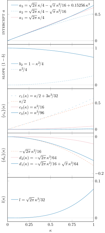
and a suitable substitution can be applied to obtain:

1n2α11/n11/ndp~(1p~)α1p~α+1.1superscript𝑛2𝛼1superscriptsubscript1𝑛11𝑛d~𝑝superscript1~𝑝𝛼1superscript~𝑝𝛼1\displaystyle\frac{1}{n^{2\alpha-1}}\int_{\nicefrac{{1}}{{n}}}^{1-\nicefrac{{1}}{{n}}}\!\!\!\!\frac{\mathop{}\!\mathrm{d}\tilde{p}}{(1-\tilde{p})^{\alpha-1}\,\tilde{p}^{\,\alpha+1}}. (82)

We proceed to split the integral for some n>1𝑛1n>1, say 2:

1/n1/2dp~(1p~)α1p~α+1+1/211/ndp~(1p~)α1p~α+1superscriptsubscript1𝑛12d~𝑝superscript1~𝑝𝛼1superscript~𝑝𝛼1superscriptsubscript1211𝑛d~𝑝superscript1~𝑝𝛼1superscript~𝑝𝛼1\displaystyle\int_{\nicefrac{{1}}{{n}}}^{\nicefrac{{1}}{{2}}}\!\!\frac{\mathop{}\!\mathrm{d}\tilde{p}}{(1-\tilde{p})^{\alpha-1}\,\tilde{p}^{\,\alpha+1}}+\int_{\nicefrac{{1}}{{2}}}^{1-\nicefrac{{1}}{{n}}}\!\!\!\!\!\!\!\!\frac{\mathop{}\!\mathrm{d}\tilde{p}}{(1-\tilde{p})^{\alpha-1}\,\tilde{p}^{\,\alpha+1}} (83)

Each of the two integrals can be bounded as follows:

1/n1/2dp~(1p~)α1p~α+1<1(11/2)α11/n1/2dp~p~α+1superscriptsubscript1𝑛12d~𝑝superscript1~𝑝𝛼1superscript~𝑝𝛼11superscript112𝛼1superscriptsubscript1𝑛12d~𝑝superscript~𝑝𝛼1\displaystyle\int_{\nicefrac{{1}}{{n}}}^{\nicefrac{{1}}{{2}}}\!\!\!\frac{\mathop{}\!\mathrm{d}\tilde{p}}{(1-\tilde{p})^{\alpha-1}\,\tilde{p}^{\,\alpha+1}}<\frac{1}{(1-\nicefrac{{1}}{{2}})^{\alpha-1}}\int_{\nicefrac{{1}}{{n}}}^{\nicefrac{{1}}{{2}}}\!\!\frac{\mathop{}\!\mathrm{d}\tilde{p}}{\tilde{p}^{\,\alpha+1}} (84a)
1/211/ndp~(1p~)α1p~α+1<1(1/2)α+11/211/ndp~(1p~)α1.superscriptsubscript1211𝑛d~𝑝superscript1~𝑝𝛼1superscript~𝑝𝛼11superscript12𝛼1superscriptsubscript1211𝑛d~𝑝superscript1~𝑝𝛼1\displaystyle\int_{\nicefrac{{1}}{{2}}}^{1-\nicefrac{{1}}{{n}}}\!\!\!\!\!\!\!\!\!\frac{\mathop{}\!\mathrm{d}\tilde{p}}{(1-\tilde{p})^{\alpha-1}\,\tilde{p}^{\,\alpha+1}}<\frac{1}{(\nicefrac{{1}}{{2}})^{\alpha+1}}\int_{\nicefrac{{1}}{{2}}}^{1-\nicefrac{{1}}{{n}}}\!\!\!\!\!\!\!\!\!\frac{\mathop{}\!\mathrm{d}\tilde{p}}{(1-\tilde{p})^{\alpha-1}}. (84b)

Evaluating these and putting everything back together, we conclude that a bound on the term (77) is given by

Υn(κ1)=κ128nm=1n11mα1(nm)α+1<κ128n(1(n1)α1+1(n+1)α+1+υ1nα1+υ2nα+1+υ3n2α1)κ12nαsubscriptΥ𝑛subscript𝜅1superscriptsubscript𝜅128𝑛superscriptsubscript𝑚1𝑛11superscript𝑚𝛼1superscript𝑛𝑚𝛼1superscriptsubscript𝜅128𝑛1superscript𝑛1𝛼11superscript𝑛1𝛼1subscript𝜐1superscript𝑛𝛼1subscript𝜐2superscript𝑛𝛼1subscript𝜐3superscript𝑛2𝛼1similar-tosuperscriptsubscript𝜅12superscript𝑛𝛼\displaystyle\Upsilon_{n}(\kappa_{1})=\frac{\kappa_{1}^{2}}{8n}\,\sum_{m=1}^{n-1}\frac{1}{m^{\alpha-1}(n-m)^{\alpha+1}}<\frac{\kappa_{1}^{2}}{8n}\Bigg{(}\!\frac{1}{(n-1)^{\alpha-1}}+\frac{1}{(n+1)^{\alpha+1}}+\frac{\upsilon_{1}}{n^{\alpha-1}}+\frac{\upsilon_{2}}{n^{\alpha+1}}+\frac{\upsilon_{3}}{n^{2\alpha-1}}\!\Bigg{)}\!\sim\frac{\kappa_{1}^{2}}{n^{\alpha}} (85)

where υisubscript𝜐𝑖\upsilon_{i} are constants. We have found that the latter two terms in eq. (75) are of the order of κ12/nαsuperscriptsubscript𝜅12superscript𝑛𝛼\kappa_{1}^{2}/n^{\alpha}. We still need to determine how this compares to the magnitude of the first term in this result, namely κ1/nα+1subscript𝜅1superscript𝑛𝛼1\kappa_{1}/n^{\alpha+1}:

κ1nα+1κ12nαnκ11.formulae-sequencegreater-than-or-equivalent-tosubscript𝜅1superscript𝑛𝛼1superscriptsubscript𝜅12superscript𝑛𝛼less-than-or-similar-to𝑛superscriptsubscript𝜅11\displaystyle\frac{\kappa_{1}}{n^{\alpha+1}}\gtrsim\frac{\kappa_{1}^{2}}{n^{\alpha}}\quad\Leftrightarrow\quad n\lesssim\kappa_{1}^{-1}. (86)

We can therefore say that for values of n𝑛n smaller than κ11superscriptsubscript𝜅11\kappa_{1}^{-1} the second and third terms are much smaller than the first and can therefore be ignored. For values of n𝑛n above this limit all terms are of comparable magnitude. However, this n¯¯𝑛\bar{n} can be related to the order of the parameters {κi}subscript𝜅𝑖\{\kappa_{i}\}:

κn¯=κ1nακ11+α<κ13.subscript𝜅¯𝑛subscript𝜅1superscript𝑛𝛼similar-tosuperscriptsubscript𝜅11𝛼superscriptsubscript𝜅13\displaystyle\kappa_{\bar{n}}=\frac{\kappa_{1}}{n^{\alpha}}\sim\kappa_{1}^{1+\alpha}<\kappa_{1}^{3}. (87)

and so ignoring these higher terms leads to an error smaller than κ13superscriptsubscript𝜅13\kappa_{1}^{3}. Therefore, we have discovered that we are free to ignore the terms discussed above, and in general ignore the interference between the magnitude of κ1subscript𝜅1\kappa_{1} and the large values of the index n𝑛n, as long as we do not concern ourselves with corrections beyond third order. We may write:

𝒄1(n)κn2n.similar-tosuperscriptsubscript𝒄1𝑛subscript𝜅𝑛2𝑛\displaystyle\bm{c}_{1}^{(n)}\sim\frac{\kappa_{n}}{2n}. (88)

As before, the constant 𝒂𝒂\bm{a} in eq. (71) can be determined if we compare our multimode ansatz to solution (70) in the buffer zone where both solutions are valid. This means expanding (70) for large x𝑥x, and comparing with eq. (71) (see eq. (91). This suggests that the value of 𝒂𝒂\bm{a} is:

𝒂=±nκnπ22n𝒂plus-or-minussubscript𝑛subscript𝜅𝑛𝜋22𝑛\displaystyle\bm{a}=\pm\sum_{n}\kappa_{n}\,\frac{\sqrt{\pi}}{2\sqrt{2n}} (89)

Our final solution with this ansatz is given by eq. (92).

To test the validity of this solution, we devise a test similar to eq. (38), but include the presence of multiple modes in the definition of the quantifier:

ϰ2(m,x)=|𝝎num𝝎(1)(x)𝝎num|m.subscriptbold-italic-ϰ2𝑚𝑥subscriptsubscript𝝎numsuperscript𝝎1𝑥subscript𝝎num𝑚\displaystyle\bm{\varkappa}_{2}(m,x)=\left|\vphantom{\Bigg{[}\Bigg{]}}\frac{\bm{\omega}_{\text{num}}-\bm{\omega}^{(1)}(x)}{\bm{\omega}_{\text{num}}}\right|_{m}. (90)

Here, 𝝎(x)𝝎𝑥\bm{\omega}(x) is given by eq. (92), 𝝎numsubscript𝝎num\bm{\omega}_{\text{num}} is the respective numerical solution, and the subscript m𝑚m signifies that all equations and solutions have been limited to the first m𝑚m terms only. In Figures 10 and 27 we demonstrate graphically the validity of our solution for m={2,5,10,20}𝑚251020m=\{2,5,10,20\} and in the intervals |x|1𝑥1|x|\leq 1 and 1x201𝑥201\leq x\leq 20, respectively.

We could try to extend this approach further, by naively including S2n(x)subscript𝑆2𝑛𝑥S_{2n}(x) terms in the ansatz. These terms, however, are redundant, as for n𝑛n ranging from 1 to ++\infty, the set {2n}2𝑛\{2n\} is a subset of {n}𝑛\{n\}, and therefore the latter terms in the sum can be absorbed into the former one. Thus, eq. (71) is the only ansatz we can use for the equation with an infinite number of modes. Finding higher-order solutions is also complicated by the fact that taking powers of the infinite sum introduces an increasing number of cross-terms.

x+nκnπ2n(±12+sin(nx2)2πnx)+𝒪(x2)𝒂+x+nκn2n1xsin(nx2)similar-to𝑥subscript𝑛subscript𝜅𝑛𝜋2𝑛plus-or-minus12𝑛superscript𝑥22𝜋𝑛𝑥𝒪superscript𝑥2𝒂𝑥subscript𝑛subscript𝜅𝑛2𝑛1𝑥𝑛superscript𝑥2\displaystyle x+\sum_{n}\kappa_{n}\frac{\sqrt{\pi}}{\sqrt{2n}}\left(\!\pm\,\frac{1}{2}+\frac{\sin\!\big{(}nx^{2}\big{)}}{\sqrt{2\pi n}\,x}\!\right)\!+\mathcal{O}\!\left(x^{-2}\right)\sim\bm{a}+x+\sum_{n}\frac{\kappa_{n}}{2n}\,\frac{1}{x}\,\sin\!\big{(}nx^{2}\big{)} (91)
𝝎1(x)=±nκnπ22n+x+nκn12n1xsin(nx2)subscript𝝎1𝑥plus-or-minussubscript𝑛subscript𝜅𝑛𝜋22𝑛𝑥subscript𝑛subscript𝜅𝑛12𝑛1𝑥𝑛superscript𝑥2\displaystyle\bm{\omega}_{1}(x)=\pm\sum_{n}\kappa_{n}\,\frac{\sqrt{\pi}}{2\sqrt{2n}}+x+\sum_{n}\kappa_{n}\,\frac{1}{2n}\,\frac{1}{x}\,\sin\!\big{(}nx^{2}\big{)} (92)
Refer to caption
Fig. 10: Graphical demonstration of the validity of solution (92) for different number of modes. Here the coefficients {κn}subscript𝜅𝑛\{\kappa_{n}\} follow the power law κ1/n2.5subscript𝜅1superscript𝑛2.5\kappa_{1}/n^{2.5}. The fractional errors scale with the value of the primary resonance modification κ1subscript𝜅1\kappa_{1}.
Refer to caption
Fig. 11: Visual representation of the integral bounds we use in the discussion of the multi-mode frequency equation. Left panel: Graph of inequality (80). Right panel: Graph of inequalities (84a) and (84b). Note that these plots show only the integrands, while the integrals we discuss are given by the area between these curves and the p~limit-from~𝑝\tilde{p}-axis.

Instead, we return to the single-mode version of the frequency equation and include a non-zero phase δχ𝛿𝜒\delta\chi:

ω(x)=1+κcos(xωδχ).superscript𝜔𝑥1𝜅𝑥𝜔𝛿𝜒\displaystyle\omega^{\prime}(x)=1+\kappa\cos\left(x\omega-\delta\chi\right). (93)

To find the solution for small |x|𝑥|x|, we can expand the cosine term on the right-hand side of the equation, and proceed in an analogous way to the zero-phase case:

ω(x)=1+κcos(δχ)cos(xω)+κsin(δχ)sin(xω).superscript𝜔𝑥1𝜅𝛿𝜒𝑥𝜔𝜅𝛿𝜒𝑥𝜔\displaystyle\omega^{\prime}(x)=1+\kappa\cos\left(\delta\chi\right)\cos\left(x\omega\right)+\kappa\sin\left(\delta\chi\right)\sin\left(x\omega\right). (94)

The zeroth-order solution is ϖ0(x)=xsubscriptitalic-ϖ0𝑥𝑥\varpi_{0}(x)=x, while higher-order solutions will differ from our previous results. The first-order function can be found from

ϖ1(x)=cos(δχ)cos(x2)+sin(δχ)sin(x2).superscriptsubscriptitalic-ϖ1𝑥𝛿𝜒superscript𝑥2𝛿𝜒superscript𝑥2\displaystyle\varpi_{1}^{\prime}(x)=\cos(\delta\chi)\cos\!\big{(}x^{2}\big{)}\!+\sin(\delta\chi)\sin\!\big{(}x^{2}\big{)}. (95)

After integrating, we arrive at the following result:

ϖ1(x)=π2(cos(δχ)C(2xπ)+sin(δχ)S(2xπ)).subscriptitalic-ϖ1𝑥𝜋2𝛿𝜒𝐶2𝑥𝜋𝛿𝜒𝑆2𝑥𝜋\displaystyle\varpi_{1}(x)=\frac{\sqrt{\pi}}{\sqrt{2}}\!\left(\vphantom{\Bigg{[}\Bigg{]}^{\!\!\!2\,}}\!\cos(\delta\chi)\,C\!\left(\!\frac{\sqrt{2}\,x}{\sqrt{\pi}}\!\right)\!+\sin(\delta\chi)\,S\!\left(\!\frac{\sqrt{2}\,x}{\sqrt{\pi}}\!\right)\!\!\right). (96)

The next-order function obeys the differential equation

ϖ2(x)=xsin(x2δχ)ϖ1(x),superscriptsubscriptitalic-ϖ2𝑥𝑥superscript𝑥2𝛿𝜒subscriptitalic-ϖ1𝑥\displaystyle\varpi_{2}^{\prime}(x)=-\,x\,\sin\!\big{(}x^{2}-\delta\chi\big{)}\,\varpi_{1}(x), (97)

and its solution is given in eq. (108). The third-order function, ϖ3(x)subscriptitalic-ϖ3𝑥\varpi_{3}(x) deserves a little more attention, as was the case for the zero-phase equation. Part of the derivative is again not integrable analytically, but could be approximated for the cases |x|1much-less-than𝑥1|x|\ll 1 and |x|1much-greater-than𝑥1|x|\gg 1, so we split the solution in two parts, given in eqs. (98) and (99).

ϖ3a(x)=π4\bigintsss0xdyy2cos(y2δχ)××(cos2(δχ)C2(2yπ)+sin2(δχ)S2(2yπ))subscriptitalic-ϖ3𝑎𝑥𝜋4superscriptsubscript\bigintsss0𝑥d𝑦superscript𝑦2superscript𝑦2𝛿𝜒superscript2𝛿𝜒superscript𝐶22𝑦𝜋superscript2𝛿𝜒superscript𝑆22𝑦𝜋\displaystyle\begin{split}&\varpi_{3a}(x)=-\frac{\pi}{4}\bigintsss_{0}^{x}\mathop{}\!\mathrm{d}y\,y^{2}\cos\!\big{(}y^{2}-\delta\chi\big{)}\,\times\\ &\quad\times\!\left(\!\vphantom{\Bigg{[}\Bigg{]}^{\!\!\!2\,}}\cos^{2}\!\left(\delta\chi\right)C^{2}\!\!\left(\!\frac{\sqrt{2}\,y}{\sqrt{\pi}}\!\right)\!+\sin^{2}\!\left(\delta\chi\right)S^{2}\!\!\left(\!\frac{\sqrt{2}\,y}{\sqrt{\pi}}\!\right)\!\!\right)\end{split} (98)

and

ϖ3b(x)=π42\bigintsss0xdyysin(2y22δχ)×\displaystyle\varpi_{3b}(x)=-\frac{\sqrt{\pi}}{4\sqrt{2}}\bigintsss_{0}^{x}\mathop{}\!\mathrm{d}y\,y\sin\!\big{(}2y^{2}-2\delta\chi\big{)}\,\times
×(cos(δχ)C(2yπ)+sin(δχ)S(2yπ))absent𝛿𝜒𝐶2𝑦𝜋𝛿𝜒𝑆2𝑦𝜋\displaystyle\quad\quad\quad\quad\times\!\left(\!\vphantom{\Bigg{[}\Bigg{]}^{\!\!\!2\,}}\cos\!\left(\delta\chi\right)C\!\left(\!\frac{\sqrt{2}\,y}{\sqrt{\pi}}\!\right)\!+\sin\!\left(\delta\chi\right)S\!\left(\!\frac{\sqrt{2}\,y}{\sqrt{\pi}}\!\right)\!\!\right)
+π8\bigintsss0xdyysin(y2δχ)×\displaystyle\quad\quad+\frac{\sqrt{\pi}}{8}\bigintsss_{0}^{x}\mathop{}\!\mathrm{d}y\,y\sin\!\big{(}y^{2}-\delta\chi\big{)}\,\times
×(cos(2δχ)C(4yπ)+sin(2δχ)S(4yπ))absent2𝛿𝜒𝐶4𝑦𝜋2𝛿𝜒𝑆4𝑦𝜋\displaystyle\quad\quad\quad\quad\times\!\left(\!\vphantom{\Bigg{[}\Bigg{]}^{\!\!\!2\,}}\cos\!\left(2\delta\chi\right)C\!\left(\!\frac{\sqrt{4}\,y}{\sqrt{\pi}}\!\right)\!+\sin\!\left(2\delta\chi\right)S\!\left(\!\frac{\sqrt{4}\,y}{\sqrt{\pi}}\!\right)\!\!\right)
+140xdyy2sin(y2δχ)14superscriptsubscript0𝑥differential-d𝑦superscript𝑦2superscript𝑦2𝛿𝜒\displaystyle\quad\quad+\frac{1}{4}\int_{0}^{x}\mathop{}\!\mathrm{d}y\,y^{2}\sin\!\left(y^{2}-\delta\chi\right) (99)

To find a solution for ϖ3a(x)subscriptitalic-ϖ3𝑎𝑥\varpi_{3a}(x), we proceed in an analogous way to the δχ=0𝛿𝜒0\delta\chi=0 case, and take the appropriate limits of interest of the Fresnel function. For |x|1much-less-than𝑥1|x|\ll 1, the expansion is a polynomial, finding an analytical approximation is straightforward, and the result is given by eq. (109). Hence the third-order solution near the origin is

ϖ3(x)=ϖ3aapprox(x)+ϖ3b(x).subscriptitalic-ϖ3𝑥subscriptitalic-ϖ3subscript𝑎approx𝑥subscriptitalic-ϖ3𝑏𝑥\displaystyle\varpi_{3}(x)=\varpi_{3a_{\rm approx}}(x)+\varpi_{3b}(x). (100)

We also calculate the asymptotic expression for ϖ3a(x)subscriptitalic-ϖ3𝑎𝑥\varpi_{3a}(x), by expanding the Fresnel function for |x|1much-greater-than𝑥1|x|\gg 1, the solution is given by eq. (110). The additive constant accounting for the value of the integral at the origin is

α=0.00991cos3(δχ)±0.08018cos2(δχ)sin(δχ)0.00185cos(δχ)sin2(δχ)±0.03110sin3(δχ)𝛼plus-or-minusminus-or-plusplus-or-minusminus-or-plus0.00991superscript3𝛿𝜒0.08018superscript2𝛿𝜒𝛿𝜒0.00185𝛿𝜒superscript2𝛿𝜒0.03110superscript3𝛿𝜒\displaystyle\begin{split}\alpha=&\mp 0.00991\cos^{3}\!\left(\delta\chi\right)\pm 0.08018\cos^{2}\!\left(\delta\chi\right)\sin\!\left(\delta\chi\right)\\ &\mp 0.00185\cos\!\left(\delta\chi\right)\sin^{2}\!\left(\delta\chi\right)\pm 0.03110\sin^{3}\!\left(\delta\chi\right)\end{split} (101)

The asymptotic expression for ϖ3(x)subscriptitalic-ϖ3𝑥\varpi_{3}(x) can be written as

ϖ3(x)=α+ϖ3aasymp(x)+ϖ3b(x).subscriptitalic-ϖ3𝑥𝛼subscriptitalic-ϖ3subscript𝑎asymp𝑥subscriptitalic-ϖ3𝑏𝑥\displaystyle\varpi_{3}(x)=\alpha+\varpi_{3a_{\rm asymp}}(x)+\varpi_{3b}(x). (102)

The validity of these solutions can be demonstrated in an analogous way to the zero-phase case, by computing:

ϰn+1=|ωnumω(n)(x)ωnum|,subscriptitalic-ϰ𝑛1subscript𝜔numsuperscript𝜔𝑛𝑥subscript𝜔num\displaystyle\varkappa_{n+1}=\left|\vphantom{\Bigg{[}\Bigg{]}}\frac{\omega_{\text{num}}-\omega^{(n)}(x)}{\omega_{\text{num}}}\right|, (103)

where ω(n)(x)superscript𝜔𝑛𝑥\omega^{(n)}(x) is the solution to eq. (93) for |x|1much-less-than𝑥1|x|\ll 1, and ωnumsubscript𝜔num\omega_{\text{num}} is the respective numerical solution. Plots of these functions for n=0,,3𝑛03n=0,\dots,3 are given in Figure 13.

Refer to caption
Fig. 12: Plot of the components of the constant a𝑎a, and plot of the combined constant for κ=0.1𝜅0.1\kappa=0.1 as functions of δχ𝛿𝜒\delta\chi.

No further calculations are needed to find the constants {bi,c1,c2,c3,d1,d2,l}subscript𝑏𝑖subscript𝑐1subscript𝑐2subscript𝑐3subscript𝑑1subscript𝑑2𝑙\{b_{i},c_{1},c_{2},c_{3},d_{1},d_{2},l\}, since we can use modified ansätze which include a phase term in their oscillating factors:

𝒮n(x)sin[n(ax+(1+b)x2δχ)]subscript𝒮𝑛𝑥𝑛𝑎𝑥1𝑏superscript𝑥2𝛿𝜒\displaystyle\mathcal{S}_{n}(x)\equiv\sin\!\left[n\Big{(}ax+\left(1+b\right)x^{2}-\delta\chi\Big{)}\vphantom{\Big{(}\Big{)}^{\!\!\!2\,}}\!\right] (104a)
𝒞n(x)cos[n(ax+(1+b)x2δχ)].subscript𝒞𝑛𝑥𝑛𝑎𝑥1𝑏superscript𝑥2𝛿𝜒\displaystyle\mathcal{C}_{n}(x)\equiv\cos\!\left[n\Big{(}ax+\left(1+b\right)x^{2}-\delta\chi\Big{)}\vphantom{\Big{(}\Big{)}^{\!\!\!2\,}}\!\right]. (104b)

To establish the constants {ai}subscript𝑎𝑖\{a_{i}\}, we match the ansatz against the new (asymptotic) solution:

ω(x)𝜔𝑥\displaystyle\omega(x) =ϖ0(x)+κϖ1(x)+κ2ϖ2(x)+κ3ϖ3(x),absentsubscriptitalic-ϖ0𝑥𝜅subscriptitalic-ϖ1𝑥superscript𝜅2subscriptitalic-ϖ2𝑥superscript𝜅3subscriptitalic-ϖ3𝑥\displaystyle=\varpi_{0}(x)+\kappa\varpi_{1}(x)+\kappa^{2}\varpi_{2}(x)+\kappa^{3}\varpi_{3}(x), (105)

where the last term is the combination of terms (102) and α𝛼\alpha is given by eq. (101). The three separate orders of the constant a𝑎a as a function of the phase difference δχ𝛿𝜒\delta\chi are:

a1=±2π4(cos(δχ)+sin(δχ))subscript𝑎1plus-or-minus2𝜋4𝛿𝜒𝛿𝜒\displaystyle a_{1}=\pm\,\frac{\sqrt{2\pi}}{4}\big{(}\!\cos\!\left(\delta\chi\right)+\sin\!\left(\delta\chi\right)\!\big{)} (106a)
a2=π16(cos(2δχ)+sin(2δχ))subscript𝑎2minus-or-plus𝜋162𝛿𝜒2𝛿𝜒\displaystyle a_{2}=\mp\,\frac{\sqrt{\pi}}{16}\big{(}\!\cos\!\left(2\delta\chi\right)+\sin\!\left(2\delta\chi\right)\!\big{)} (106b)
a3= 0.00991cos3(δχ)±0.08018cos2(δχ)sin(δχ)subscript𝑎3plus-or-minusminus-or-plus0.00991superscript3𝛿𝜒0.08018superscript2𝛿𝜒𝛿𝜒\displaystyle a_{3}=\mp\,0.00991\cos^{3}\!\left(\delta\chi\right)\pm 0.08018\cos^{2}\!\left(\delta\chi\right)\sin\!\left(\delta\chi\right)
0.00185cos(δχ)sin2(δχ)±0.03110sin3(δχ)plus-or-minusminus-or-plus0.00185𝛿𝜒superscript2𝛿𝜒0.03110superscript3𝛿𝜒\displaystyle\quad\quad\quad\mp 0.00185\cos\!\left(\delta\chi\right)\sin^{2}\!\left(\delta\chi\right)\pm 0.03110\sin^{3}\!\left(\delta\chi\right)
±2π256(cos(3δχ)sin(3δχ).\displaystyle\quad\quad\quad\pm\frac{\sqrt{2\pi}}{256}\big{(}\!\cos\!\left(3\delta\chi\right)-\sin\!\left(3\delta\chi\right)\big{.}
.+7cos(δχ)+7sin(δχ))\displaystyle\quad\quad\quad\quad\quad\quad\quad\quad\quad\quad\quad\big{.}+7\cos\!\left(\delta\chi\right)+7\sin\!\left(\delta\chi\right)\!\big{)}
±6π768(3cos(3δχ)+3sin(3δχ).\displaystyle\quad\quad\quad\pm\frac{\sqrt{6\pi}}{768}\big{(}3\cos\!\left(3\delta\chi\right)+3\sin\!\left(3\delta\chi\right)\big{.}
.+cos(δχ)sin(δχ))\displaystyle\quad\quad\quad\quad\quad\quad\quad\quad\quad\quad\quad\big{.}+\cos\!\left(\delta\chi\right)-\sin\!\left(\delta\chi\right)\!\big{)}
±2π3/2128(cos(δχ)sin(δχ))plus-or-minus2superscript𝜋32128𝛿𝜒𝛿𝜒\displaystyle\quad\quad\quad\pm\frac{\sqrt{2}\,\pi^{\nicefrac{{3}}{{2}}}}{128}\big{(}\!\cos\!\left(\delta\chi\right)-\sin\!\left(\delta\chi\right)\!\big{)} (106c)

The constant a𝑎a itself is given by

a=a1κ+a2κ2+a3κ3𝑎subscript𝑎1𝜅subscript𝑎2superscript𝜅2subscript𝑎3superscript𝜅3\displaystyle a=a_{1}\kappa+a_{2}\kappa^{2}+a_{3}\kappa^{3} (107)

Plots of these functions are given in Figure 12.

ϖ2(x)=π22cos(x2δχ)(cos(δχ)C(2xπ)+sin(δχ)S(2xπ))π8(cos(2δχ)C(4xπ)+sin(2δχ)S(4xπ))x4subscriptitalic-ϖ2𝑥𝜋22superscript𝑥2𝛿𝜒𝛿𝜒𝐶2𝑥𝜋𝛿𝜒𝑆2𝑥𝜋𝜋82𝛿𝜒𝐶4𝑥𝜋2𝛿𝜒𝑆4𝑥𝜋𝑥4\displaystyle\begin{split}&\varpi_{2}(x)=\frac{\sqrt{\pi}}{2\sqrt{2}}\,\cos\!\big{(}x^{2}-\delta\chi\big{)}\!\!\left(\vphantom{\Bigg{[}\Bigg{]}^{\!\!\!2\,}}\!\cos(\delta\chi)\,C\!\left(\!\frac{\sqrt{2}\,x}{\sqrt{\pi}}\!\right)\!+\sin(\delta\chi)\,S\!\left(\!\frac{\sqrt{2}\,x}{\sqrt{\pi}}\!\right)\!\!\right)\\ &\quad\quad\quad\quad\quad\quad\quad\quad\quad\quad\quad\quad\quad\quad\quad\quad\quad\quad\quad\quad\quad\quad\quad\quad-\frac{\sqrt{\pi}}{8}\!\left(\vphantom{\Bigg{[}\Bigg{]}^{\!\!\!2\,}}\!\cos(2\delta\chi)\,C\!\left(\!\frac{\sqrt{4}\,x}{\sqrt{\pi}}\!\right)\!+\sin(2\delta\chi)\,S\!\left(\!\frac{\sqrt{4}\,x}{\sqrt{\pi}}\!\right)\!\!\right)\!-\frac{x}{4}\end{split} (108)
ϖ3aapprox(x)=(33cos2(δχ)353sin2(δχ))[2π64(cos(δχ)C(2xπ)+sin(δχ)S(2xπ))132xcos(x2δχ)148x3sin(x2δχ)]+(15cos2(δχ)19sin2(δχ))[78x5cos(x2δχ)+14x7sin(x2δχ)]subscriptitalic-ϖ3subscript𝑎approx𝑥33superscript2𝛿𝜒353superscript2𝛿𝜒2𝜋64𝛿𝜒𝐶2𝑥𝜋𝛿𝜒𝑆2𝑥𝜋132𝑥superscript𝑥2𝛿𝜒148superscript𝑥3superscript𝑥2𝛿𝜒15superscript2𝛿𝜒19superscript2𝛿𝜒delimited-[]78superscript𝑥5superscript𝑥2𝛿𝜒14superscript𝑥7superscript𝑥2𝛿𝜒\displaystyle\begin{split}&\varpi_{3a_{\rm approx}}(x)=\left(\!\vphantom{\Bigg{[}\Bigg{]}}33\cos^{2}\!\left(\delta\chi\right)-\frac{35}{3}\sin^{2}\!\left(\delta\chi\right)\!\right)\!\!\left[\vphantom{\left[\Bigg{[}\Bigg{]}^{\!\!\!2\,}\right]^{\!\!\!2\,}}\frac{\sqrt{2\pi}}{64}\!\left(\!\vphantom{\Bigg{[}\Bigg{]}^{\!\!\!2\,}}\cos\!\left(\delta\chi\right)C\!\left(\!\frac{\sqrt{2}\,x}{\sqrt{\pi}}\!\right)\!+\sin\!\left(\delta\chi\right)S\!\left(\!\frac{\sqrt{2}\,x}{\sqrt{\pi}}\!\right)\!\!\right)\!-\frac{1}{32}\,x\cos\!\big{(}x^{2}-\delta\chi\big{)}\right.\\ &\quad\quad\quad\quad\quad\quad\quad\quad\left.\vphantom{\left[\Bigg{[}\Bigg{]}^{\!\!\!2\,}\right]^{\!\!\!2\,}}-\frac{1}{48}\,x^{3}\sin\!\big{(}x^{2}-\delta\chi\big{)}\!\right]\!+\left(\!\vphantom{\Bigg{[}\Bigg{]}}\frac{1}{5}\cos^{2}\!\left(\delta\chi\right)-\frac{1}{9}\sin^{2}\!\left(\delta\chi\right)\!\right)\!\!\left[\vphantom{\Bigg{[}\Bigg{]}}\frac{7}{8}\,x^{5}\cos\!\big{(}x^{2}-\delta\chi\big{)}+\frac{1}{4}\,x^{7}\sin\!\big{(}x^{2}-\delta\chi\big{)}\!\right]\end{split} (109)
ϖ3aasymp(x)=±2π32(cos3(δχ)+sin3(δχ))ln|x|2π64sin(2δχ)(cos(δχ)sin(δχ))(x2+34x2)2π64(cos3(δχ)C(2xπ)+sin3(δχ)S(2xπ))32π128sin(2δχ)(cos(δχ)S(2xπ)+sin(δχ)C(2xπ))+2π3/264(cos(δχ)S(2xπ)sin(δχ)C(2xπ))+6π192cos(2δχ)(cos(δχ)C(6xπ)+sin(δχ)S(6xπ))π32xsin(x2δχ)±2π64(11x4)(cos2(δχ)cos(2x2δχ)+sin2(δχ)sin(2x2δχ))±2π1281x2(cos2(δχ)sin(2x2δχ)sin2(δχ)cos(2x2δχ))1641x3cos(2δχ)(cos(x2+δχ)+13cos(3x2δχ))5128sin(2δχ)cos(x2+δχ)x532561x5cos(2δχ)(sin(3x2δχ)+sin(x2+δχ))subscriptitalic-ϖ3subscript𝑎asymp𝑥minus-or-plusplus-or-minus2𝜋32superscript3𝛿𝜒superscript3𝛿𝜒𝑥2𝜋642𝛿𝜒𝛿𝜒𝛿𝜒superscript𝑥234superscript𝑥22𝜋64superscript3𝛿𝜒𝐶2𝑥𝜋superscript3𝛿𝜒𝑆2𝑥𝜋32𝜋1282𝛿𝜒𝛿𝜒𝑆2𝑥𝜋𝛿𝜒𝐶2𝑥𝜋2superscript𝜋3264𝛿𝜒𝑆2𝑥𝜋𝛿𝜒𝐶2𝑥𝜋6𝜋1922𝛿𝜒𝛿𝜒𝐶6𝑥𝜋𝛿𝜒𝑆6𝑥𝜋plus-or-minus𝜋32𝑥superscript𝑥2𝛿𝜒2𝜋6411superscript𝑥4superscript2𝛿𝜒2superscript𝑥2𝛿𝜒superscript2𝛿𝜒2superscript𝑥2𝛿𝜒plus-or-minus2𝜋1281superscript𝑥2superscript2𝛿𝜒2superscript𝑥2𝛿𝜒superscript2𝛿𝜒2superscript𝑥2𝛿𝜒1641superscript𝑥32𝛿𝜒superscript𝑥2𝛿𝜒133superscript𝑥2𝛿𝜒51282𝛿𝜒superscript𝑥2𝛿𝜒superscript𝑥532561superscript𝑥52𝛿𝜒3superscript𝑥2𝛿𝜒superscript𝑥2𝛿𝜒\displaystyle\begin{split}&\varpi_{3a_{\rm asymp}}(x)=\pm\,\frac{\sqrt{2\pi}}{32}\left(\cos^{3}\!\left(\delta\chi\right)+\sin^{3}\!\left(\delta\chi\right)\right)\ln\!|x|\mp\frac{\sqrt{2\pi}}{64}\,\sin\!\left(2\delta\chi\right)\!\big{(}\!\cos\!\left(\delta\chi\right)-\sin\!\left(\delta\chi\right)\!\big{)}\!\left(\!x^{2}+\frac{3}{4x^{2}}\!\right)\\ &\quad\quad\quad\quad\quad\quad\quad\quad-\frac{\sqrt{2\pi}}{64}\!\left(\!\vphantom{\Bigg{[}\Bigg{]}^{\!\!\!2\,}}\cos^{3}\!\left(\delta\chi\right)C\!\left(\!\frac{\sqrt{2}\,x}{\sqrt{\pi}}\!\right)\!+\sin^{3}\!\left(\delta\chi\right)S\!\left(\!\frac{\sqrt{2}\,x}{\sqrt{\pi}}\!\right)\!\!\right)\\ &\quad\quad\quad\quad\quad\quad\quad\quad\quad\quad-\frac{3\sqrt{2\pi}}{128}\sin\!\left(2\delta\chi\right)\!\left(\!\vphantom{\Bigg{[}\Bigg{]}^{\!\!\!2\,}}\cos\!\left(\delta\chi\right)S\!\left(\!\frac{\sqrt{2}\,x}{\sqrt{\pi}}\!\right)\!+\sin\!\left(\delta\chi\right)C\!\left(\!\frac{\sqrt{2}\,x}{\sqrt{\pi}}\!\right)\!\!\right)\\ &\quad\quad\quad\quad\quad\quad\quad\quad\quad\quad\quad\quad+\frac{\sqrt{2}\,\pi^{\nicefrac{{3}}{{2}}}}{64}\!\left(\!\vphantom{\Bigg{[}\Bigg{]}^{\!\!\!2\,}}\cos\!\left(\delta\chi\right)S\!\left(\!\frac{\sqrt{2}\,x}{\sqrt{\pi}}\!\right)\!-\sin\!\left(\delta\chi\right)C\!\left(\!\frac{\sqrt{2}\,x}{\sqrt{\pi}}\!\right)\!\!\right)\\ &\quad\quad\quad\quad\quad\quad\quad\quad\quad\quad\quad\quad\quad\quad+\frac{\sqrt{6\pi}}{192}\cos\!\left(2\delta\chi\right)\!\left(\!\vphantom{\Bigg{[}\Bigg{]}^{\!\!\!2\,}}\cos\!\left(\delta\chi\right)C\!\left(\!\frac{\sqrt{6}\,x}{\sqrt{\pi}}\!\right)\!+\sin\!\left(\delta\chi\right)S\!\left(\!\frac{\sqrt{6}\,x}{\sqrt{\pi}}\!\right)\!\!\right)\\ &\quad\quad\quad\quad\quad\quad\quad-\frac{\pi}{32}\,x\sin\!\left(x^{2}-\delta\chi\right)\pm\frac{\sqrt{2\pi}}{64}\!\left(\!1-\frac{1}{x^{4}}\!\right)\!\left(\cos^{2}\!\left(\delta\chi\right)\cos\!\left(2x^{2}-\delta\chi\right)+\sin^{2}\!\left(\delta\chi\right)\sin\!\left(2x^{2}-\delta\chi\right)\!\right)\\ &\quad\quad\quad\quad\quad\quad\quad\quad\pm\frac{\sqrt{2\pi}}{128}\,\frac{1}{x^{2}}\!\left(\cos^{2}\!\left(\delta\chi\right)\sin\!\left(2x^{2}-\delta\chi\right)-\sin^{2}\!\left(\delta\chi\right)\cos\!\left(2x^{2}-\delta\chi\right)\!\right)\\ &\quad\quad\quad\quad\quad\quad\quad\quad\quad\quad-\frac{1}{64}\,\frac{1}{x^{3}}\cos\!\left(2\delta\chi\right)\!\left(\cos\!\left(x^{2}+\delta\chi\right)+\frac{1}{3}\cos\!\left(3x^{2}-\delta\chi\right)\!\right)\\ &\quad\quad\quad\quad\quad\quad\quad\quad\quad\quad\quad\quad-\frac{5}{128}\sin\!\left(2\delta\chi\right)\frac{\cos\!\left(x^{2}+\delta\chi\right)}{x^{5}}-\frac{3}{256}\,\frac{1}{x^{5}}\cos\!\left(2\delta\chi\right)\!\left(\sin\!\left(3x^{2}-\delta\chi\right)\!+\sin\!\left(x^{2}+\delta\chi\right)\!\right)\end{split} (110)
ϖ3b(x)=2π32cos[2(x2δχ)](cos(δχ)C(2xπ)+sin(δχ)S(2xπ))π16cos(x2δχ)(cos(2δχ)C(4xπ)+sin(2δχ)S(4xπ))+6π192(cos(3δχ)C(6xπ)+sin(3δχ)S(6xπ))+52π64(cos(δχ)C(2xπ)+sin(δχ)S(2xπ))18xcos(x2δχ)subscriptitalic-ϖ3𝑏𝑥2𝜋322superscript𝑥2𝛿𝜒𝛿𝜒𝐶2𝑥𝜋𝛿𝜒𝑆2𝑥𝜋𝜋16superscript𝑥2𝛿𝜒2𝛿𝜒𝐶4𝑥𝜋2𝛿𝜒𝑆4𝑥𝜋6𝜋1923𝛿𝜒𝐶6𝑥𝜋3𝛿𝜒𝑆6𝑥𝜋52𝜋64𝛿𝜒𝐶2𝑥𝜋𝛿𝜒𝑆2𝑥𝜋18𝑥superscript𝑥2𝛿𝜒\displaystyle\begin{split}&\varpi_{3b}(x)=\frac{\sqrt{2\pi}}{32}\cos\!\left[2(x^{2}-\delta\chi)\right]\!\!\left(\!\vphantom{\Bigg{[}\Bigg{]}^{\!\!\!2\,}}\cos\!\left(\delta\chi\right)C\!\left(\!\frac{\sqrt{2}\,x}{\sqrt{\pi}}\!\right)\!+\sin\!\left(\delta\chi\right)S\!\left(\!\frac{\sqrt{2}\,x}{\sqrt{\pi}}\!\right)\!\!\right)\\ &\quad\quad\quad\quad\quad\quad-\frac{\sqrt{\pi}}{16}\cos\!\left(x^{2}-\delta\chi\right)\!\!\left(\!\vphantom{\Bigg{[}\Bigg{]}^{\!\!\!2\,}}\cos\!\left(2\delta\chi\right)C\!\left(\!\frac{\sqrt{4}\,x}{\sqrt{\pi}}\!\right)\!+\sin\!\left(2\delta\chi\right)S\!\left(\!\frac{\sqrt{4}\,x}{\sqrt{\pi}}\!\right)\!\!\right)\\ &\quad\quad\quad\quad\quad\quad\quad\quad+\frac{\sqrt{6\pi}}{192}\!\left(\!\vphantom{\Bigg{[}\Bigg{]}^{\!\!\!2\,}}\cos\!\left(3\delta\chi\right)C\!\left(\!\frac{\sqrt{6}\,x}{\sqrt{\pi}}\!\right)\!+\sin\!\left(3\delta\chi\right)S\!\left(\!\frac{\sqrt{6}\,x}{\sqrt{\pi}}\!\right)\!\!\right)\\ &\quad\quad\quad\quad\quad\quad\quad\quad\quad\quad+\frac{5\sqrt{2\pi}}{64}\!\left(\!\vphantom{\Bigg{[}\Bigg{]}^{\!\!\!2\,}}\cos\!\left(\delta\chi\right)C\!\left(\!\frac{\sqrt{2}\,x}{\sqrt{\pi}}\!\right)\!+\sin\!\left(\delta\chi\right)S\!\left(\!\frac{\sqrt{2}\,x}{\sqrt{\pi}}\!\right)\!\!\right)\!-\frac{1}{8}\,x\cos\!\left(x^{2}-\delta\chi\right)\end{split} (111)
ω3(x)=(a1κ+a2κ2+a3κ3)+(1κ24)x+κ121xsin[(a1κ+a2κ2)x+(1κ24)x2δχ]subscript𝜔3𝑥subscript𝑎1𝜅subscript𝑎2superscript𝜅2subscript𝑎3superscript𝜅31superscript𝜅24𝑥𝜅121𝑥subscript𝑎1𝜅subscript𝑎2superscript𝜅2𝑥1superscript𝜅24superscript𝑥2𝛿𝜒\displaystyle\omega_{3}(x)=\big{(}a_{1}\kappa+a_{2}\kappa^{2}+a_{3}\kappa^{3}\big{)}\!+\left(\!\vphantom{\Bigg{[}\Bigg{]}}1-\frac{\kappa^{2}}{4}\!\right)\!x+\kappa\,\frac{1}{2}\,\frac{1}{x}\,\sin\!\left[\vphantom{\Bigg{[}\Bigg{]}^{\!\!\!2\,}}\!\left(a_{1}\kappa+a_{2}\kappa^{2}\right)\!x+\!\Bigg{(}\!1-\frac{\kappa^{2}}{4}\!\Bigg{)}x^{2}-\delta\chi\right]
+κ21161xsin[2(a1κx+x2δχ)]+κ31x(332sin(x2δχ)+196sin[3(x2δχ)])superscript𝜅21161𝑥2subscript𝑎1𝜅𝑥superscript𝑥2𝛿𝜒superscript𝜅31𝑥332superscript𝑥2𝛿𝜒1963superscript𝑥2𝛿𝜒\displaystyle\quad+\kappa^{2}\frac{1}{16}\,\frac{1}{x}\,\sin\!\Big{[}2\!\left(a_{1}\kappa\,x+x^{2}-\delta\chi\right)\!\Big{]}\!+\kappa^{3}\,\frac{1}{x}\!\left(\!\vphantom{\Bigg{[}\Bigg{]}}\frac{3}{32}\,\sin\!\left(x^{2}-\delta\chi\right)+\frac{1}{96}\,\sin\!\Big{[}3\big{(}x^{2}-\delta\chi\big{)}\Big{]}\!\right) (112)
κ22π161x2sin(a1κx+x2δχ)±κ3(π641x2sin(x2δχ)2π641x2sin[2(x2δχ)]+2π32ln|x|).plus-or-minusminus-or-plussuperscript𝜅22𝜋161superscript𝑥2subscript𝑎1𝜅𝑥superscript𝑥2𝛿𝜒superscript𝜅3𝜋641superscript𝑥2superscript𝑥2𝛿𝜒2𝜋641superscript𝑥22superscript𝑥2𝛿𝜒2𝜋32𝑥\displaystyle\quad\quad\mp\kappa^{2}\frac{\sqrt{2\pi}}{16}\,\frac{1}{x^{2}}\,\sin\!\left(a_{1}\kappa\,x+x^{2}-\delta\chi\right)\!\pm\kappa^{3}\!\left(\!\vphantom{\Bigg{[}\Bigg{]}}\frac{\sqrt{\pi}}{64}\,\frac{1}{x^{2}}\,\sin\!\left(x^{2}-\delta\chi\right)-\frac{\sqrt{2\pi}}{64}\,\frac{1}{x^{2}}\,\sin\!\Big{[}2\big{(}x^{2}-\delta\chi\big{)}\Big{]}+\frac{\sqrt{2\pi}}{32}\,\ln\!|x|\!\right).
Refer to caption
Fig. 13: Graphical demonstration of the validity of solutions ϖ0(x)=xsubscriptitalic-ϖ0𝑥𝑥\varpi_{0}(x)=x, (96), (108), and (100). In each plot we have used κ=0.1𝜅0.1\kappa=0.1. It is evident that the fractional errors scale with the value of the resonance modification κ𝜅\kappa, and for each order n𝑛n of the solution, the remainder is of order 𝒪(κn+1)𝒪superscript𝜅𝑛1\mathcal{O}\!\left(\kappa^{n+1}\right).

Solutions ϖ0(x)subscriptitalic-ϖ0𝑥\varpi_{0}(x), ϖ1(x)subscriptitalic-ϖ1𝑥\varpi_{1}(x), ϖ2(x)subscriptitalic-ϖ2𝑥\varpi_{2}(x) and ϖ3(x)subscriptitalic-ϖ3𝑥\varpi_{3}(x) are plotted in Fig. (9), while a more rigorous derivation of the principle we use here is presented in Appendix IV. This paves the way for finding a solution to the general equation with an infinite number of modes.

Before we proceed with this, we check graphically the validity of solution (112). Fig. 14 depicts the fractional errors ϰ4(x)subscriptitalic-ϰ4𝑥\varkappa_{4}(x) for the usual values of κ𝜅\kappa, and for 4 different values of the initial phase offset.

Finally, we consider the multi-mode frequency equation with a non-vanishing initial phase:

𝝎(x)=1+nκncos(nxω𝝎δχn),superscript𝝎𝑥1subscript𝑛subscript𝜅𝑛𝑛subscript𝑥𝜔𝝎𝛿subscript𝜒𝑛\displaystyle\bm{\omega}^{\prime}(x)=1+\sum_{n}\kappa_{n}\cos\!\left(nx_{\omega}\,\bm{\omega}-\delta\chi_{n}\right), (19a)

where the array of constants {δχn}𝛿subscript𝜒𝑛\{\delta\chi_{n}\} is known and can in principle be computed from the constants of motion through eq. (16). Before proceeding, we elect to write the equation out in the following more revealing way

𝝎(x)=1+nκncos(δχn)cos(nxω𝝎)+κnsin(δχn)sin(nxω𝝎).superscript𝝎𝑥1subscript𝑛subscript𝜅𝑛𝛿subscript𝜒𝑛𝑛subscript𝑥𝜔𝝎subscript𝜅𝑛𝛿subscript𝜒𝑛𝑛subscript𝑥𝜔𝝎\displaystyle\begin{split}\bm{\omega}^{\prime}(x)=1+\sum_{n}\kappa_{n}&\cos\!\left(\delta\chi_{n}\right)\cos\!\left(nx_{\omega}\,\bm{\omega}\right)\\ &+\kappa_{n}\sin\!\left(\delta\chi_{n}\right)\sin\!\left(nx_{\omega}\,\bm{\omega}\right).\end{split} (113)

For small |x|𝑥|x|, we find consecutively:

ϖ0(x)=xsubscriptbold-italic-ϖ0𝑥𝑥\displaystyle\bm{\varpi}_{0}(x)=x (114)

and

ϖ1,n(x)=π2n(cos(δχn)C(2nxπ)+sin(δχn)S(2nxπ))subscriptbold-italic-ϖ1𝑛𝑥𝜋2𝑛𝛿subscript𝜒𝑛𝐶2𝑛𝑥𝜋𝛿subscript𝜒𝑛𝑆2𝑛𝑥𝜋\displaystyle\begin{split}&\bm{\varpi}_{1,n}(x)=\frac{\sqrt{\pi}}{\sqrt{2n}}\!\left(\!\cos(\delta\chi_{n})\,C\!\left(\!\frac{\sqrt{2n}\,x}{\sqrt{\pi}}\!\right)\vphantom{\Bigg{[}\Bigg{]}^{\!\!\!2\,}}\right.\\ &\quad\quad\quad\quad\quad\quad\quad\quad\quad\quad\left.\vphantom{\Bigg{[}\Bigg{]}^{\!\!\!2\,}}+\sin(\delta\chi_{n})\,S\!\left(\!\frac{\sqrt{2n}\,x}{\sqrt{\pi}}\!\right)\!\!\right)\end{split} (115)

As before, higher-order solutions are not necessary, so we can write the solution for |x|1much-less-than𝑥1|x|\ll 1 as

𝝎1(x)=ϖ0(x)+nκnϖ1,n(x).subscript𝝎1𝑥subscriptbold-italic-ϖ0𝑥subscript𝑛superscript𝜅𝑛subscriptbold-italic-ϖ1𝑛𝑥\displaystyle\bm{\omega}_{1}(x)=\bm{\varpi}_{0}(x)+\sum_{n}\kappa^{n}\bm{\varpi}_{1,n}(x). (116)
Refer to caption
Fig. 14: Graphical demonstration of the validity of solution (112) for several characteristic values of κ𝜅\kappa and for sample values of the phase angle δχ𝛿𝜒\delta\chi.

Next we choose an elaborate ansatz of the form:

𝝎1(x)=𝒂+(1+𝒃)x+n𝒄n𝒮n(x)xsubscript𝝎1𝑥𝒂1𝒃𝑥subscript𝑛subscript𝒄𝑛subscript𝒮𝑛𝑥𝑥\displaystyle\bm{\omega}_{1}(x)=\bm{a}+\left(1+\bm{b}\right)x+\sum_{n}\bm{c}_{n}\frac{\mathcal{S}_{n}(x)}{x} (117)

where we note that we neglect terms of 𝒪(x2)𝒪superscript𝑥2\mathcal{O}\!\left(x^{-2}\right), which correspond to oscillations which die out quickly with |x|𝑥|x|. The derivative of this ansatz is given by

𝝎1(x)=1+𝒃+2(1+𝒃)nn𝒄n𝒞n(x).superscriptsubscript𝝎1𝑥1𝒃21𝒃subscript𝑛𝑛subscript𝒄𝑛subscript𝒞𝑛𝑥\displaystyle\bm{\omega}_{1}^{\prime}(x)=1+\bm{b}+2\left(1+\bm{b}\right)\sum_{n}n\,\bm{c}_{n}\,\mathcal{C}_{n}(x). (118)

This needs to match the right-hand side of eq. (19a). We perform analysis similar to our earlier discussion on the zero-phase multi-mode version to find the solution (121). Note that the slope correction is still zero at leading order, and we discover that the constants {δχn}𝛿subscript𝜒𝑛\{\delta\chi_{n}\} only appear in the argument of the oscillation modes. The constant 𝒂𝒂\bm{a} is found by comparing the above ansatz with the |x|1much-greater-than𝑥1|x|\gg 1 limit of solution (116).

𝒂=±nκnπ22n(cos(δχn)+sin(δχn))𝒂plus-or-minussubscript𝑛subscript𝜅𝑛𝜋22𝑛𝛿subscript𝜒𝑛𝛿subscript𝜒𝑛\displaystyle\bm{a}=\pm\sum_{n}\kappa_{n}\frac{\sqrt{\pi}}{2\sqrt{2n}}\,\big{(}\!\cos(\delta\chi_{n})+\sin(\delta\chi_{n})\big{)} (119)

Validating these solutions can be done in the same manner as earlier, by computing the quantities analogous to eq. (38) and eq. (90), but this time incorporating the phase variable into the checks. These are depicted in Figures 15 and 28. For these figures, we have assumed that the phases {δχn}𝛿subscript𝜒𝑛\{\delta\chi_{n}\} cycle the set {0,π/2,π,3π/2}0𝜋2𝜋3𝜋2\{0,\pi/2,\pi,3\pi/2\},

δχn=(δχ1+(n1)π/2)mod2π𝛿subscript𝜒𝑛modulo𝛿subscript𝜒1𝑛1𝜋22𝜋\displaystyle\delta\chi_{n}=\big{(}\delta\chi_{1}+(n-1)\,\nicefrac{{\pi}}{{2}}\big{)}\mod 2\pi (120)

As before, it is very challenging to correctly determine higher-order solutions in terms of the parameters {κn}subscript𝜅𝑛\{\kappa_{n}\} as higher order corrections include contributions from cross-terms between modes, which significantly complicate the analysis. Instead, we will focus on the more interesting phase resonance equation, where this problem is avoided, and higher-order solutions can still be found in the multi-mode case.

𝝎1(x)=±nκnπ22n(cos(δχn)+sin(δχn))+x+nκn12n1xsin(nx2δχn).subscript𝝎1𝑥plus-or-minussubscript𝑛subscript𝜅𝑛𝜋22𝑛𝛿subscript𝜒𝑛𝛿subscript𝜒𝑛𝑥subscript𝑛subscript𝜅𝑛12𝑛1𝑥𝑛superscript𝑥2𝛿subscript𝜒𝑛\displaystyle\bm{\omega}_{1}(x)=\pm\sum_{n}\kappa_{n}\frac{\sqrt{\pi}}{2\sqrt{2n}}\,\big{(}\!\cos(\delta\chi_{n})+\sin(\delta\chi_{n})\big{)}+x+\sum_{n}\kappa_{n}\,\frac{1}{2n}\,\frac{1}{x}\,\sin\!\big{(}nx^{2}-\delta\chi_{n}\big{)}. (121)
Refer to caption
Fig. 15: Graphical demonstration of the validity of solution (121) for different number of terms on the right-hand side and for values of {δχn}𝛿subscript𝜒𝑛\{\delta\chi_{n}\} given by eq. (120). In all panels we have used κ1=0.1subscript𝜅10.1\kappa_{1}=0.1 with consecutive values given by κn=κ1/n2.5subscript𝜅𝑛subscript𝜅1superscript𝑛2.5\kappa_{n}=\kappa_{1}/n^{2.5}.

This concludes our discussion of the frequency resonance equation. We have produced a series of solutions with increasing generality, and have provided graphical evidence of their validity. We note that some results have been intentionally left to Appendix F, since they are simple extensions of less general cases presented within this Section. We can now turn our attention to the phase resonance equation and its solutions.

IV.3 Phase resonance equation

The phase-resonance equation is derived in Section II and makes use of the action-angle variables {qμ}subscript𝑞𝜇\{q_{\mu}\}, instead of the fundamental frequencies {ωμ}subscript𝜔𝜇\{\omega_{\mu}\} to write down the Fourier modes of the self-force function. In the case of a multitude of modes in this expansion, as well as a non-vanishing initial phase offset, the equation takes the form

ϕ′′(x)=1+n>0λncos(nϕδψn).superscriptitalic-ϕ′′𝑥1subscript𝑛0subscript𝜆𝑛𝑛italic-ϕ𝛿subscript𝜓𝑛\displaystyle\phi^{\prime\prime}(x)=1+\sum_{n>0}\lambda_{n}\cos\!\left(n\phi-\delta\psi_{n}\right). (19b)

Similarly to our approach to the frequency resonance equation, we examine the case in which we ignore all higher-order modes beyond the first one (n=1𝑛1n=1), and assume a zero initial phase, so eq. (19b) simplifies to

ϕ′′(x)=1+λcos(ϕ(x)).superscriptitalic-ϕ′′𝑥1𝜆italic-ϕ𝑥\displaystyle\phi^{\prime\prime}(x)=1+\lambda\cos\!\big{(}\phi(x)\big{)}. (122)

The equation is again non-linear due to the additive constant, and an analytic solution cannot be provided in the general case. Instead we employ an iterative approach to establish a series of solutions in increasing order of the mode parameter λλ11𝜆subscript𝜆1much-less-than1\lambda\equiv\lambda_{1}\ll 1. At first, we ignore the term involving λ𝜆\lambda, and seek a solution to the equation:

ϕ0′′(x)=1+𝒪(λ),superscriptsubscriptitalic-ϕ0′′𝑥1𝒪𝜆\displaystyle\phi_{0}^{\prime\prime}(x)=1+\mathcal{O}\!\left(\lambda\right), (123)

which straightforwardly yields the zeroth-order solution to the phase resonance equation (this and higher order solutions are denote by PH) in the current regime

ϕ0(x)=x22.subscriptitalic-ϕ0𝑥superscript𝑥22\displaystyle\phi_{0}(x)=\frac{x^{2}}{2}. (124)

Further solutions are obtained by substituting the current solution on the right-hand side of the source equation (122), while on the left-hand side we include this solution plus the next-order correction. In the general case, we would need to solve the equation (for n1𝑛1n\geq 1)

ϕn′′(x)=1+λcos(ϕn1(x)),superscriptsubscriptitalic-ϕ𝑛′′𝑥1𝜆subscriptitalic-ϕ𝑛1𝑥\displaystyle\phi_{n}^{\prime\prime}(x)=1+\lambda\cos\!\left(\phi_{n-1}(x)\right), (125)

where ϕn(x)subscriptitalic-ϕ𝑛𝑥\phi_{n}(x) is the complete nthsuperscript𝑛thn^{\text{th}}-order solution. We apply this iterative technique to find the first-order correction: we use the function ϕ0(x)subscriptitalic-ϕ0𝑥\phi_{0}(x) as the source for the next order solution ϕ1(x)=ϕ0(x)+ϕ(1)(x)subscriptitalic-ϕ1𝑥subscriptitalic-ϕ0𝑥subscriptitalic-ϕ1𝑥\phi_{1}(x)=\phi_{0}(x)+\phi_{(1)}(x). That means we write ϕ0(x)subscriptitalic-ϕ0𝑥\phi_{0}(x) as the argument on the right-hand side, while on the left-hand side we solve for ϕ1(x)subscriptitalic-ϕ1𝑥\phi_{1}(x), a combination of the zeroth-order ϕ0(x)subscriptitalic-ϕ0𝑥\phi_{0}(x) and the first-order correction ϕ(1)(x)subscriptitalic-ϕ1𝑥\phi_{(1)}(x). Throughout our current discussion, we shall use ϕn(x)subscriptitalic-ϕ𝑛𝑥\phi_{n}(x) to denote the complete solution to order n𝑛n, while ϕ(n)(x)subscriptitalic-ϕ𝑛𝑥\phi_{(n)}(x) would denote the nthsuperscript𝑛thn^{\text{th}}-order correction to ϕ0(x)subscriptitalic-ϕ0𝑥\phi_{0}(x), i.e. ϕn(x)=ϕ0(x)+ϕ(n)(x)subscriptitalic-ϕ𝑛𝑥subscriptitalic-ϕ0𝑥subscriptitalic-ϕ𝑛𝑥\phi_{n}(x)=\phi_{0}(x)+\phi_{(n)}(x). Using this, we write:

ϕ1′′(x)=(ϕ0+ϕ(1))′′=1+ϕ(1)′′=1+λcos(ϕ0).superscriptsubscriptitalic-ϕ1′′𝑥superscriptsubscriptitalic-ϕ0subscriptitalic-ϕ1′′1superscriptsubscriptitalic-ϕ1′′1𝜆subscriptitalic-ϕ0\displaystyle\phi_{1}^{\prime\prime}(x)=\left(\phi_{0}+\phi_{(1)}\right)^{\prime\prime}=1+\phi_{(1)}^{\prime\prime}=1+\lambda\cos\!\left(\phi_{0}\right). (126)

From this, we find a differential equation for ϕ(1)(x)subscriptitalic-ϕ1𝑥\phi_{(1)}(x):

ϕ(1)′′(x)=λcos(x22).superscriptsubscriptitalic-ϕ1′′𝑥𝜆superscript𝑥22\displaystyle\phi_{(1)}^{\prime\prime}(x)=\lambda\cos\!\left(\!\frac{x^{2}}{2}\!\vphantom{\Bigg{[}\Bigg{]}}\right). (127)

The details of finding this solution are described in Appendix I, here we only quote the final result:

ϕ(1)(x)=λ[πxC(xπ)sin(x22)].subscriptitalic-ϕ1𝑥𝜆delimited-[]𝜋𝑥𝐶𝑥𝜋superscript𝑥22\displaystyle\phi_{(1)}(x)=\lambda\!\left[\vphantom{\Bigg{[}\Bigg{]}^{\!\!\!2\,}}\sqrt{\pi}\,x\,C\!\left(\!\frac{x}{\sqrt{\pi}}\!\right)\!-\sin\!\Bigg{(}\!\frac{x^{2}}{2}\!\vphantom{\Bigg{[}\Bigg{]}}\Bigg{)}\!\right]. (128)

Combining this with ϕ0(x)subscriptitalic-ϕ0𝑥\phi_{0}(x), we find the complete first-order-in-λ𝜆\lambda solution to eq. (122), given by (LABEL:eq:phase_solution_1). It is worth explaining that the solution has been rearranged into a form which is more useful for our discussion later on. More specifically, we have grouped together terms which oscillate around the value ϕ(x)=0italic-ϕ𝑥0\phi(x)=0 – both (C(

)
1/2
)
minus-or-plus𝐶

12
(C\!\left(\mathchoice{{\hbox to4.99995pt{\hss\leavevmode\hbox{\set@color\raisebox{0.0pt}{\scalebox{2.0}{\raisebox{0.0pt}{$\displaystyle\cdot$}}}}\hss}}}{{\hbox to4.99995pt{\hss\leavevmode\hbox{\set@color\raisebox{0.0pt}{\scalebox{2.0}{\raisebox{0.0pt}{$\textstyle\cdot$}}}}\hss}}}{{\hbox to4.16661pt{\hss\leavevmode\hbox{\set@color\raisebox{0.0pt}{\scalebox{2.0}{\raisebox{0.0pt}{$\scriptstyle\cdot$}}}}\hss}}}{{\hbox to3.61105pt{\hss\leavevmode\hbox{\set@color\raisebox{0.0pt}{\scalebox{2.0}{\raisebox{0.0pt}{$\scriptscriptstyle\cdot$}}}}\hss}}}\right)\mp\nicefrac{{1}}{{2}})
and sin(

)

\sin(\mathchoice{{\hbox to4.99995pt{\hss\leavevmode\hbox{\set@color\raisebox{0.0pt}{\scalebox{2.0}{\raisebox{0.0pt}{$\displaystyle\cdot$}}}}\hss}}}{{\hbox to4.99995pt{\hss\leavevmode\hbox{\set@color\raisebox{0.0pt}{\scalebox{2.0}{\raisebox{0.0pt}{$\textstyle\cdot$}}}}\hss}}}{{\hbox to4.16661pt{\hss\leavevmode\hbox{\set@color\raisebox{0.0pt}{\scalebox{2.0}{\raisebox{0.0pt}{$\scriptstyle\cdot$}}}}\hss}}}{{\hbox to3.61105pt{\hss\leavevmode\hbox{\set@color\raisebox{0.0pt}{\scalebox{2.0}{\raisebox{0.0pt}{$\scriptscriptstyle\cdot$}}}}\hss}}})
are such functions (see Appendix D for details about the former). Moreover, we have collected the terms proportional to x2superscript𝑥2x^{2} and x𝑥x into a single quadratic term (by completing the square, which inevitably introduces a further constant, however it is of second order in the mode parameter λ𝜆\lambda, and not relevant here). Hence the solution is comprised of a modified (shifted along the x𝑥x-axis) quadratic term and a term ρ1subscript𝜌1\rho_{1} which oscillates around ϕ=0italic-ϕ0\phi=0, and whose frequency of oscillations increases with the value of x𝑥x.

A number of results in this section contain the symbols “±plus-or-minus\pm” and “minus-or-plus\mp”. Similarly to the discussion of the solutions of the frequency resonance equation, these do not signify two alternative equations, but rather that the lower signs are valid for x0𝑥0x\leq 0, while the upper signs hold for x0𝑥0x\geq 0, both part of the same solution. It is important to note that for large values of x𝑥x, the oscillating terms become small, and the approximate slope of ϕ1(x)subscriptitalic-ϕ1𝑥\phi_{1}(x) is given by πλ/2𝜋𝜆2\sqrt{\pi}\,\lambda/2. We will see later how this slope evolves when we add higher-order-in-λ𝜆\lambda terms, but for now let us denote σ1(λ)=λ/2subscript𝜎1𝜆𝜆2\sigma_{1}(\lambda)=\lambda/2, which is the shift in the position of the leading parabolic term.
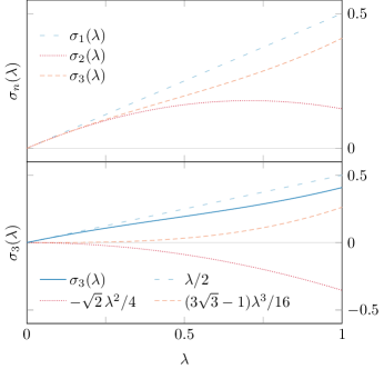
Refer to caption
Fig. 16: Evolution of the slope of the phase resonance solutions. The domain of the plot shows all possible values for the mode parameter: 0λ10𝜆10\leq\lambda\leq 1. Upper panel: the evolution of the slope for all three solutions which have been calculated explicitly in the paper. Lower panel: the individual components which make up the slope function σ3(λ)subscript𝜎3𝜆\sigma_{3}(\lambda).

Applying the same iterative approach, we use the combined function ϕ1(x)subscriptitalic-ϕ1𝑥\phi_{1}(x) as the source for the second-order asymptotic solution ϕ2(x)=ϕ0(x)+ϕ(2)(x)subscriptitalic-ϕ2𝑥subscriptitalic-ϕ0𝑥subscriptitalic-ϕ2𝑥\phi_{2}(x)=\phi_{0}(x)+\phi_{(2)}(x), where the second-order correction ϕ(2)(x)subscriptitalic-ϕ2𝑥\phi_{(2)}(x) is comprised both of first- and second- order terms. This notation is convenient since ϕ0′′(x)=1superscriptsubscriptitalic-ϕ0′′𝑥1\phi_{0}^{\prime\prime}(x)=1 cancels with the constant term on the right-hand side, and upon integrating twice, we obtain an expression for ϕ(2)(x)subscriptitalic-ϕ2𝑥\phi_{(2)}(x), the complete solution to second order in λ𝜆\lambda, only without the zeroth-order quadratic term. On the right-hand side, we substitute the complete first-order solution, ϕ1(x)=ϕ0(x)+ϕ(1)(x)subscriptitalic-ϕ1𝑥subscriptitalic-ϕ0𝑥subscriptitalic-ϕ1𝑥\phi_{1}(x)=\phi_{0}(x)+\phi_{(1)}(x),

ϕ(2)′′(x)=λcos(ϕ0+ϕ(1)).superscriptsubscriptitalic-ϕ2′′𝑥𝜆subscriptitalic-ϕ0subscriptitalic-ϕ1\displaystyle\phi_{(2)}^{\prime\prime}(x)=\lambda\,\cos\!\left(\phi_{0}+\phi_{(1)}\right). (129)

In fact, from eqs. (127) and (129) we can infer the general form of this differential equation (for n>1𝑛1n>1):

ϕ(n)′′(x)=(ϕnϕ0)′′(x)==λcos(ϕn1)=λcos(ϕ0+ϕ(n1)).superscriptsubscriptitalic-ϕ𝑛′′𝑥superscriptsubscriptitalic-ϕ𝑛subscriptitalic-ϕ0′′𝑥𝜆subscriptitalic-ϕ𝑛1𝜆subscriptitalic-ϕ0subscriptitalic-ϕ𝑛1\displaystyle\begin{split}\phi_{(n)}^{\prime\prime}(x)&=\left(\phi_{n}-\phi_{0}\right)^{\prime\prime}\!(x)=\\ &=\lambda\cos\!\left(\phi_{n-1}\right)=\lambda\cos\!\left(\phi_{0}+\phi_{(n-1)}\right).\end{split} (130)

The details involved in solving eq. (129) are presented in Appendix I, together with the full-form solution. Here, we omit these details, and simply quote the final combined result ϕ2(x)=ϕ0(x)+ϕ(2)(x)subscriptitalic-ϕ2𝑥subscriptitalic-ϕ0𝑥subscriptitalic-ϕ2𝑥\phi_{2}(x)=\phi_{0}(x)+\phi_{(2)}(x) in the form of a modified quadratic term, plus two terms, both of them 𝒪(λ2)𝒪superscript𝜆2\mathcal{O}\!\left(\lambda^{2}\right) that oscillate and remain small for all x𝑥x.

ϕ2(x)=π2\StrLen[\arglen]([xπ±[12λ24λ2]])2+λρ1(xπ±σ1(λ))+λ2ρ2(xπ).subscriptitalic-ϕ2𝑥𝜋2\StrLendelimited-[]\arglensuperscriptabsentdelimited-[]plus-or-minus𝑥𝜋delimited-[]12𝜆24superscript𝜆22𝜆subscript𝜌1plus-or-minus𝑥𝜋subscript𝜎1𝜆superscript𝜆2subscript𝜌2𝑥𝜋\displaystyle\begin{split}\phi_{2}(x)&=\frac{\pi}{2}\!\StrLen{}[\arglen]\left(\vphantom{\left[\frac{x}{\sqrt{\pi}}\pm\left[\frac{1}{2}\,\lambda-\frac{\sqrt{2}}{4}\,\lambda^{2}\right]\right]^{\!\!\!2\,}}\!\!\sqrt{\vphantom{|}}\!\left[\frac{x}{\sqrt{\pi}}\pm\left[\frac{1}{2}\,\lambda-\frac{\sqrt{2}}{4}\,\lambda^{2}\right]\right]\!\right)^{\!\!\!2\,}\!+\lambda\,\rho_{1}\!\!\left(\!\frac{x}{\sqrt{\pi}}\!\pm\sigma_{1}(\lambda)\!\right)+\lambda^{2}\rho_{2}\!\!\left(\!\frac{x}{\sqrt{\pi}}\!\right).\end{split} (131)

We note some interesting features of this solution. Most notably, the shift in the quadratic x𝑥x term has changed from σ1(λ)=λ/2subscript𝜎1𝜆𝜆2\sigma_{1}(\lambda)=\lambda/2 to σ2(λ)=λ/22λ2/4subscript𝜎2𝜆𝜆22superscript𝜆24\sigma_{2}(\lambda)=\lambda/2-\sqrt{2}\,\lambda^{2}/4 (and the slope for large |x|𝑥|x| has changed from πσ1(λ)𝜋subscript𝜎1𝜆\sqrt{\pi}\,\sigma_{1}(\lambda) to πσ2(λ)𝜋subscript𝜎2𝜆\sqrt{\pi}\,\sigma_{2}(\lambda)). The term which is proportional to λ𝜆\lambda has the same functional form as the corresponding term in solution (LABEL:eq:phase_solution_1), however we see that in (131) each instance of x/π𝑥𝜋x/\!\sqrt{\pi} has been modified by exactly ±σ1(λ)plus-or-minussubscript𝜎1𝜆\pm\sigma_{1}(\lambda). We also have a new class of terms, all of which also oscillate around the x𝑥x-axis, and they are proportional to λ2superscript𝜆2\lambda^{2}. We will investigate the numerical performance of these solutions after we explore the next-order solution.

The solutions presented in Gair, Yunes, and Bender (2012) do not continue further than this order. Since our goal is to solve the multi-mode equation (19b), as a form of sanity check, we would like to present the solution to third order in the single-mode parameter λ𝜆\lambda, i.e. the solution to the following generating equation:

ϕ3′′(x)=1+λcos(ϕ2(x))superscriptsubscriptitalic-ϕ3′′𝑥1𝜆subscriptitalic-ϕ2𝑥\displaystyle\phi_{3}^{\prime\prime}(x)=1+\lambda\cos\!\big{(}\phi_{2}(x)\big{)} (132)

The solution follows via the same technique as the previous two, and again it is not practical to present the details of the derivation here. Instead, the reader is invited to consult Appendix I for the technicalities of the calculation as well as the full solution without abbreviations. With every successive iteration we obtain new terms, and we have grouped them together in a similar fashion to before. Here we have terms which are proportional to λ3superscript𝜆3\lambda^{3}, as well as modified terms, originating from the lower-order solutions. The result (133) is the complete solution to third order, for a single mode with amplitude λ𝜆\lambda, with vanishing initial phase δψ=0𝛿𝜓0\delta\psi=0.

ϕ3(x)=subscriptitalic-ϕ3𝑥absent\displaystyle\phi_{3}(x)= π2\StrLen[\arglen]([xπ±[12λ24λ2+33116λ3]])2+λρ1(xπ±σ2(λ))+λ2ρ2(xπ±σ1(λ))+λ3ρ3(xπ)𝜋2\StrLendelimited-[]\arglensuperscriptabsentdelimited-[]plus-or-minus𝑥𝜋delimited-[]12𝜆24superscript𝜆233116superscript𝜆32𝜆subscript𝜌1plus-or-minus𝑥𝜋subscript𝜎2𝜆superscript𝜆2subscript𝜌2plus-or-minus𝑥𝜋subscript𝜎1𝜆superscript𝜆3subscript𝜌3𝑥𝜋\displaystyle\,\frac{\pi}{2}\!\StrLen{}[\arglen]\left(\vphantom{\left[\frac{x}{\sqrt{\pi}}\pm\left[\frac{1}{2}\,\lambda-\frac{\sqrt{2}}{4}\,\lambda^{2}+\frac{3\sqrt{3}-1}{16}\,\lambda^{3}\right]\right]^{\!\!\!2\,}}\!\!\sqrt{\vphantom{|}}\!\left[\frac{x}{\sqrt{\pi}}\pm\left[\frac{1}{2}\,\lambda-\frac{\sqrt{2}}{4}\,\lambda^{2}+\frac{3\sqrt{3}-1}{16}\,\lambda^{3}\right]\right]\!\right)^{\!\!\!2\,}\!+\lambda\,\rho_{1}\!\!\left(\!\frac{x}{\sqrt{\pi}}\!\pm\sigma_{2}(\lambda)\!\right)+\lambda^{2}\rho_{2}\!\!\left(\!\frac{x}{\sqrt{\pi}}\!\pm\sigma_{1}(\lambda)\!\right)+\lambda^{3}\rho_{3}\!\!\left(\!\frac{x}{\sqrt{\pi}}\!\right) (133)

In (133), the x𝑥x-shift of the quadratic term is now

σ3(λ)=12λ24λ2+33116λ3,subscript𝜎3𝜆12𝜆24superscript𝜆233116superscript𝜆3\displaystyle\sigma_{3}(\lambda)=\frac{1}{2}\,\lambda-\frac{\sqrt{2}}{4}\,\lambda^{2}+\frac{3\sqrt{3}-1}{16}\,\lambda^{3}, (134)

and consequently, the slope of the graph for large x𝑥x is given by πσ3(λ)𝜋subscript𝜎3𝜆\sqrt{\pi}\,\sigma_{3}(\lambda). In fact Gair et al. (2012) numerically computed the change in the slope of the phase solution at λ3superscript𝜆3\lambda^{3} order:

ϕ3(x)π2λπ22λ2+0.4648λ3+𝒪(λ4).similar-tosuperscriptsubscriptitalic-ϕ3𝑥𝜋2𝜆𝜋22superscript𝜆20.4648superscript𝜆3𝒪superscript𝜆4\displaystyle\phi_{3}^{\prime}(x)\sim\frac{\sqrt{\pi}}{2}\,\lambda-\frac{\sqrt{\pi}}{2\sqrt{2}}\,\lambda^{2}+0.4648\,\lambda^{3}+\mathcal{O}\!\left(\lambda^{4}\right). (135)

As a form of consistency check, we can directly compare this with the (analytically derived) factor multiplying the λ3superscript𝜆3\lambda^{3} term in the coefficient of x𝑥x in eq. (133) and confirm that both numerical values agree:

π×33116λ30.4648λ3.𝜋33116superscript𝜆30.4648superscript𝜆3\displaystyle\sqrt{\pi}\times\frac{3\sqrt{3}-1}{16}\,\lambda^{3}\approx 0.4648\,\lambda^{3}. (136)

Moreover, we can notice a parallel between the terms proportional to λ𝜆\lambda in each of (LABEL:eq:phase_solution_1) — (133): all three brackets have the same dependence on x𝑥x, meaning that for λ=0𝜆0\lambda=0, they would be equal. However, in each of them, each instance of x/π𝑥𝜋x/\!\sqrt{\pi} is modified by a different function of the mode parameter λ𝜆\lambda. Compared to (LABEL:eq:phase_solution_1), each x/π𝑥𝜋x/\!\sqrt{\pi} in (131) is shifted by ±σ1(λ)plus-or-minussubscript𝜎1𝜆\pm\,\sigma_{1}(\lambda), and in (133), it is shifted by ±σ2(λ)plus-or-minussubscript𝜎2𝜆\pm\,\sigma_{2}(\lambda). Similar evolution can be noticed in the terms proportional to λ2superscript𝜆2\lambda^{2} in (131) and (133). In the latter, each instance of a term involving x𝑥x is shifted by σ1(λ)subscript𝜎1𝜆\sigma_{1}(\lambda) compared to the former. While it is hard to predict what terms at higher order would look like, because the x𝑥x-dependence cannot be inferred from the first three solutions, we can nevertheless expect that at fourth order, the term proportional to λ3superscript𝜆3\lambda^{3} would look similar to its counterpart in (133), with each x/π𝑥𝜋x/\!\sqrt{\pi} term modified by ±σ1(λ)plus-or-minussubscript𝜎1𝜆\pm\,\sigma_{1}(\lambda), and so on. It is evident that the functions σn(λ)subscript𝜎𝑛𝜆\sigma_{n}(\lambda) play an important role in the phase resonance solutions, and at least in the evolution of the slope of the graph for large |x|𝑥|x|. In Figure 16, we plot these functions and present what they look like for different values of λ𝜆\lambda.

Let us investigate the properties of solutions (124) — (133): each of them contains a quadratic term of the form π/2(x/π±σi)2𝜋2superscriptplus-or-minus𝑥𝜋subscript𝜎𝑖2\pi/2\,(x/\!\sqrt{\pi}\pm\sigma_{i})^{2}. Since the magnitudes of the rest of the terms in each solution scale with λnsuperscript𝜆𝑛\lambda^{n}, the functions look similar when plotted together, as can be seen in Figure 31. It is hard to distinguish them in this plot, unless we zoom in closely on a region. For example, if we focus on the region around x=0𝑥0x=0 we see that while ϕ0(x)=x2/2subscriptitalic-ϕ0𝑥superscript𝑥22\phi_{0}(x)=x^{2}/2 goes through the origin, the rest of the solutions deviate slightly from zero. This is due to the fact that a perturbative solution of order n𝑛n is only approximate, and is correct up to a remainder of 𝒪(λn+1)𝒪superscript𝜆𝑛1\mathcal{O}\!\left(\lambda^{n+1}\right). Indeed, if we consider each solution ϕ{1,2,3}(x)subscriptitalic-ϕ123𝑥\phi_{\{1,2,3\}}(x) for x=0𝑥0x=0:

ϕ1(0)=π8λ2,ϕ2(0)=π(128λ3+116λ4),ϕ3(0)=π(3342+132λ4364264λ5+2863512λ6)formulae-sequencesubscriptitalic-ϕ10𝜋8superscript𝜆2formulae-sequencesubscriptitalic-ϕ20𝜋128superscript𝜆3116superscript𝜆4subscriptitalic-ϕ30𝜋3342132superscript𝜆4364264superscript𝜆52863512superscript𝜆6\displaystyle\phi_{1}(0)=\frac{\pi}{8}\,\lambda^{2},\;\phi_{2}(0)=\pi\Bigg{(}\!\frac{1-\sqrt{2}}{8}\,\lambda^{3}+\frac{1}{16}\,\lambda^{4}\!\Bigg{)},\;\phi_{3}(0)=\pi\Bigg{(}\!\frac{3\sqrt{3}-4\sqrt{2}+1}{32}\,\lambda^{4}-\frac{3\sqrt{6}-4-\sqrt{2}}{64}\,\lambda^{5}+\frac{28-6\sqrt{3}}{512}\,\lambda^{6}\!\Bigg{)}

we find that they are indeed of the expected order in each case (see Figure 17 for a plot of these functions). These expressions have further higher order corrections coming from sub-leading order terms in the expansion of Fresnel cosine integrals (see eq. (175b) in Appendix D). Since these solutions are hard to examine graphically, we need to employ other techniques to compare the accuracy of the solutions. Specifically, we compare them with a purely numerical solution of the phase equation.
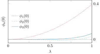
Refer to caption
Fig. 17: Plot of the functions ϕ{1,2,3}(0)subscriptitalic-ϕ1230\phi_{\{1,2,3\}}(0) as functions of λ𝜆\lambda.

A simple plot like the lower one in Fig. 31 shows that our highest-order solution, eq. (133), does indeed compare well — within 𝒪(λ4)𝒪superscript𝜆4\mathcal{O}\!\left(\lambda^{4}\right) — to a purely numerical solution (Wolfram Research, Inc., ). We need to quantify the comparison between this numerical solution and our analytical solutions as the mode parameter λ𝜆\lambda varies.

Refer to caption
Fig. 18: Graphical demonstration of the validity of the phase resonance solution for 4 different values of the parameter λ𝜆\lambda. The remainders {ϑn(x)}subscriptitalic-ϑ𝑛𝑥\{\vartheta_{n}(x)\} are normalised by x𝑥x in order to remove the linear trend. It is evident that the remainders scale with the value of the resonance modification λ𝜆\lambda, and for each order n𝑛n of the solution, the remainder is of order 𝒪(λn+1)𝒪superscript𝜆𝑛1\mathcal{O}\!\left(\lambda^{n+1}\right).

It is important to demonstrate that each of the corrections ϕ(n)(x)subscriptitalic-ϕ𝑛𝑥\phi_{(n)}(x) appropriately captures all of the behaviour of the solution up to order 𝒪(λn)𝒪superscript𝜆𝑛\mathcal{O}\!\left(\lambda^{n}\right), i.e., that the difference between the full numerical solution ϕnum(x)subscriptitalic-ϕnum𝑥\phi_{\text{num}}(x) and the correction is of order 𝒪(λn+1)𝒪superscript𝜆𝑛1\mathcal{O}\!\left(\lambda^{n+1}\right) at most. To do this, we employ a technique that allows us to solve numerically for that difference (instead of naively subtracting each analytical solution from the numerical map). Consider eq. (122) which is our initial source equation:

ϕ′′(x)=1+λcos(ϕ(x)).superscriptitalic-ϕ′′𝑥1𝜆italic-ϕ𝑥\displaystyle\phi^{\prime\prime}(x)=1+\lambda\cos\!\big{(}\phi(x)\big{)}. (122)

As per our recipe, we would substitute the highest-known-order solution ϕn(x)subscriptitalic-ϕ𝑛𝑥\phi_{n}(x) on the right-hand side, and solve the equation for the next-order solution ϕn+1(x)subscriptitalic-ϕ𝑛1𝑥\phi_{n+1}(x). In reality, the solution we are looking for appears on either side of the equation, and furthermore the functions ϕ(x)italic-ϕ𝑥\phi(x) also contain the orders beyond n𝑛n which we have so far been ignoring in eqs. (125) and (130):

ϕ(x)=ϕ0(x)+ϕ(n)(x)+ϑn+1(x).italic-ϕ𝑥subscriptitalic-ϕ0𝑥subscriptitalic-ϕ𝑛𝑥subscriptitalic-ϑ𝑛1𝑥\displaystyle\phi(x)=\phi_{0}(x)+\phi_{(n)}(x)+\vartheta_{n+1}(x). (137)

Here, ϕ0(x)=x2/2subscriptitalic-ϕ0𝑥superscript𝑥22\phi_{0}(x)=x^{2}/2 and ϕ(n)(x)subscriptitalic-ϕ𝑛𝑥\phi_{(n)}(x) is the correction to ϕ0subscriptitalic-ϕ0\phi_{0}. ϑn+1(x)subscriptitalic-ϑ𝑛1𝑥\vartheta_{n+1}(x) is the remainder of the complete solution which is not included into ϕn(x)subscriptitalic-ϕ𝑛𝑥\phi_{n}(x). We can easily find a generic equation satisfied by the functions ϑn+1(x)subscriptitalic-ϑ𝑛1𝑥\vartheta_{n+1}(x) by using expression (137) in eq. (122) and making use of eq. (122). In general, ϑn+1(x)subscriptitalic-ϑ𝑛1𝑥\vartheta_{n+1}(x) satisfies the differential equation

ϑn+1′′(x)=λcos(ϕn+ϑn+1(x))ϕ(n)′′(x).superscriptsubscriptitalic-ϑ𝑛1′′𝑥𝜆subscriptitalic-ϕ𝑛subscriptitalic-ϑ𝑛1𝑥superscriptsubscriptitalic-ϕ𝑛′′𝑥\displaystyle\vartheta_{n+1}^{\prime\prime}(x)=\lambda\cos\!\left(\phi_{n}+\vartheta_{n+1}(x)\right)-\phi_{(n)}^{\prime\prime}(x). (138)

For n=0𝑛0n=0 we can find directly from the source equation

ϑ1′′(x)=λcos(ϕ0(x)+ϑ1(x)).superscriptsubscriptitalic-ϑ1′′𝑥𝜆subscriptitalic-ϕ0𝑥subscriptitalic-ϑ1𝑥\displaystyle\vartheta_{1}^{\prime\prime}(x)=\lambda\cos\!\left(\phi_{0}(x)+\vartheta_{1}(x)\right). (139)

By solving for ϑn+1(x)subscriptitalic-ϑ𝑛1𝑥\vartheta_{n+1}(x) and confirming that the result is 𝒪(λn+1)x𝒪superscript𝜆𝑛1for-all𝑥\mathcal{O}\!\left(\lambda^{n+1}\right)\forall x we verify that ϕn(x)subscriptitalic-ϕ𝑛𝑥\phi_{n}(x) capture the complete 𝒪(λn)𝒪superscript𝜆𝑛\mathcal{O}\!\left(\lambda^{n}\right) behaviour. The plots for ϑn(x)/xsubscriptitalic-ϑ𝑛𝑥𝑥\vartheta_{n}(x)/x (to remove the expected linear-in-x𝑥x general trend) are shown in Figure 18, where we have performed the computation for 4 distinct values of λ𝜆\lambda: 0.1,0.05,0.01,0.10.050.010.1,0.05,0.01, and 0.0050.0050.005.

The corrections ϕ(n)(x)subscriptitalic-ϕ𝑛𝑥\phi_{(n)}(x) themselves are plotted (for λ(1)=0.1superscript𝜆10.1\lambda^{(1)}=0.1) in Figure 32, found in the Appendix. Similarly, plots of the oscillating functions ρ1(x)subscript𝜌1𝑥\rho_{1}(x), ρ2(x)subscript𝜌2𝑥\rho_{2}(x), and ρ3(x)subscript𝜌3𝑥\rho_{3}(x) can be found in Figures 33, 34, and 35, respectively, with other relevant discussions in Appendix II.

Refer to caption
Fig. 19: The third-order correction to the phase resonance equation for different values of the mode number r𝑟r. These solutions all have mode parameters λr=0.1subscript𝜆𝑟0.1\lambda_{r}=0.1, so the graph only reflects the effect which the number of the mode has on the solution.

Before moving on to the case of multiple modes, it is intriguing to look into several other toy models. So far we have only looked at the resonance equation with a single mode n=1𝑛1n=1. We now consider the same equation, but with the sole mode n=r𝑛𝑟n=r on the right-hand side. The leading-order solution is still (124).

(ϕ(r)(x))′′=1+λrcos(rϕ).superscriptsuperscriptitalic-ϕ𝑟𝑥′′1subscript𝜆𝑟𝑟italic-ϕ\displaystyle\left(\phi^{(r)}(x)\right)^{\prime\prime}=1+\lambda_{r}\cos\!\left(r\phi\right). (140)

The explicit solution of the above equation is redundant, since it can be obtained from eq. (122) by setting

and therefore its corrections could be obtained from eqs. (LABEL:eq:phase_solution_1) – (133) by applying these transformations. The explicit form of the solutions is presented in Appendix III. In Figure 19 we show these solutions (at third order, i.e. complete) for different values of the mode number r𝑟r. The modified σ𝜎\sigma-terms are presented in Figure 36, while the numerical validation of these solutions can be found in Figure 37.

Another toy model which deserves attention is the case of two distinct modes on the right-hand side:

(ϕ(r,s)(x))′′=1+λrcos(rϕ)+λscos(sϕ).superscriptsuperscriptitalic-ϕ𝑟𝑠𝑥′′1subscript𝜆𝑟𝑟italic-ϕsubscript𝜆𝑠𝑠italic-ϕ\displaystyle\left(\phi^{(r,s)}(x)\right)^{\prime\prime}=1+\lambda_{r}\cos\!\left(r\phi\right)+\lambda_{s}\cos\!\left(s\phi\right). (142)

The leading-order solution is unchanged, while the higher-order corrections are presented in Appendix IV. We note that at first order, the correction is just the sum of the corrections due to each of the separate oscillating modes on the right-hand side. This, however, is not the case at higher order, where cross-terms appear. It is important to note that these cross-terms are not sub-leading to the other quadratic terms in the solution. This is in contrast to the frequency-resonance equation, where these cross-terms were sub-leading in this respect (see Appendix III). In Figure 38 we can examine the σ𝜎\sigma-terms associated with this equation, while the validity of the solutions is presented in Figure 39.

Our objective in this paper is to extend this approach beyond the scope which has been developed thus far. So far we have explored the solution to third order in the mode parameter. However, we are still limited to the case of a single mode, and we are assuming that the initial phase is ϕ(0)=0italic-ϕ00\phi(0)=0. We now relax the first of these restrictions and allow for an infinite number of oscillating modes, each with a distinct parameter λisubscript𝜆𝑖\lambda_{i}. This is achieved through allowing for multiple modes in the Fourier expansion, thus lifting the assumption that the contribution derives primarily from the first Fourier mode.
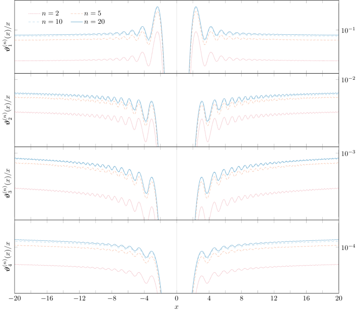
Refer to caption
Fig. 20: Graphical demonstration of the validity of solutions (144), (147), (247), and (249). All these solutions are for λ1=0.1subscript𝜆10.1\lambda_{1}=0.1, but include numbers of modes. The λ𝜆\lambda parameters follow the law λn=λ1/n2.5subscript𝜆𝑛subscript𝜆1superscript𝑛2.5\lambda_{n}=\lambda_{1}/n^{2.5}.

We derived the phase resonance equation in Section II. In the regime of an unrestricted number of oscillating modes, still assuming that the initial phase is 0, the form of the phase resonance equation is given by

ϕ′′(x)=1+nλncos(nϕ)superscriptbold-italic-ϕ′′𝑥1subscript𝑛subscript𝜆𝑛𝑛bold-italic-ϕ\displaystyle\bm{\phi}^{\prime\prime}(x)=1+\sum_{n}\lambda_{n}\cos\left(n\bm{\phi}\right) (143)

Similar to the previous equation under consideration, this is a second order non-linear differential equation, and therefore finding an exact solution is not possible, and a perturbative solution quickly grows to become heavily involved. For brevity, here we only present the final solutions, while details about the solutions and relevant discussion are collected in Appendix G. At zero’th order in the mode parameters {λn}subscript𝜆𝑛\{\lambda_{n}\}, we ignore any oscillating terms on the right-hand side, and the resulting differential equation is identical to that in the single-mode case, eq. (123); the solution is obtained by integrating twice:

ϕ0′′=1ϕ0(x)=x22formulae-sequencesuperscriptsubscriptbold-italic-ϕ0′′1subscriptbold-italic-ϕ0𝑥superscript𝑥22\displaystyle\bm{\phi}_{0}^{\prime\prime}=1\quad\Leftrightarrow\quad\bm{\phi}_{0}(x)=\frac{x^{2}}{2} (144)

Building onto this result, we construct the equivalent to eq. (125), which in the multi-mode case is now given by

ϕm+1′′(x)=1+nλncos(nϕm(x)).superscriptsubscriptbold-italic-ϕ𝑚1′′𝑥1subscript𝑛subscript𝜆𝑛𝑛subscriptbold-italic-ϕ𝑚𝑥\displaystyle\bm{\phi}_{m+1}^{\prime\prime}(x)=1+\sum_{n}\lambda_{n}\cos\big{(}n\,\bm{\phi}_{m}(x)\big{)}. (145)

We will solve this consecutively for m=0,1𝑚01m=0,1 and 2, and we will obtain the respective solutions to the phase resonance equation for the multi-mode case. At first instance, we use ϕ0(x)=x2/2subscriptbold-italic-ϕ0𝑥superscript𝑥22\bm{\phi}_{0}(x)=x^{2}/2 as the argument of the trigonometric function on the right-hand side, and investigate the solution to this equation to first order in {λn}subscript𝜆𝑛\{\lambda_{n}\}, which will yield the first-order correction ϕ(1)(x)subscriptbold-italic-ϕ1𝑥\bm{\phi}_{(1)}(x):

ϕ(1)′′(x)=nλncos(nϕ0)superscriptsubscriptbold-italic-ϕ1′′𝑥subscript𝑛subscript𝜆𝑛𝑛subscriptbold-italic-ϕ0\displaystyle\bm{\phi}_{(1)}^{\prime\prime}(x)=\sum_{n}\lambda_{n}\cos\left(n\bm{\phi}_{0}\right) (146)

The details of finding the first-order correction can be found in Appendix V. Combining ϕ(1)(x)subscriptbold-italic-ϕ1𝑥\bm{\phi}_{(1)}(x) with (144), we establish the complete first-order solution.

ϕ1(x)=π2(xπ±12nλnn)2+nλnn𝝆1n\StrLen[\arglen]([xπ]).subscriptbold-italic-ϕ1𝑥𝜋2superscriptplus-or-minus𝑥𝜋12subscript𝑛subscript𝜆𝑛𝑛2subscript𝑛subscript𝜆𝑛𝑛superscriptsubscript𝝆1𝑛\StrLendelimited-[]\arglenabsentdelimited-[]𝑥𝜋\displaystyle\bm{\phi}_{1}(x)=\frac{\pi}{2}\!\left(\!\frac{x}{\sqrt{\pi}}\pm\frac{1}{2}\sum_{n}\frac{\lambda_{n}}{\sqrt{n}}\!\right)^{\!\!\!2\,}+\sum_{n}\frac{\lambda_{n}}{n}\,\bm{\rho}_{1}^{n}\!\StrLen{}[\arglen]\left(\vphantom{\left[\frac{x}{\sqrt{\pi}}\right]^{\!\!\!2\,}}\!\!\sqrt{\vphantom{|}}\!\left[\frac{x}{\sqrt{\pi}}\right]\!\right). (147)

Here 𝝆1n(x)superscriptsubscript𝝆1𝑛𝑥\bm{\rho}_{1}^{n}(x) is an oscillating term proportional to |λ|𝜆|\lambda|, equivalent to ρ1(x)subscript𝜌1𝑥\rho_{1}(x), and given explicitly in Appendix I. Compared to (144), eq. (147) has a modified quadratic term and a part which oscillates around 0 for all x𝑥x.

We apply the same technique to find the second-order solution, namely ϕ(2)(x)subscriptbold-italic-ϕ2𝑥\bm{\phi}_{(2)}(x), which contains terms that are quadratic in the parameters {λn}subscript𝜆𝑛\{\lambda_{n}\}. Similarly to previous iterations, we use the current highest-order solution ϕ1(x)subscriptbold-italic-ϕ1𝑥\bm{\phi}_{1}(x) to establish a differential equation for ϕ(2)(x)subscriptbold-italic-ϕ2𝑥\bm{\phi}_{(2)}(x). The differential equation we want to solve is given by

ϕ(2)′′(x)=nλncos(nϕ1(x))superscriptsubscriptbold-italic-ϕ2′′𝑥subscript𝑛subscript𝜆𝑛𝑛subscriptbold-italic-ϕ1𝑥\displaystyle\bm{\phi}_{(2)}^{\prime\prime}(x)=\sum_{n}\lambda_{n}\cos\big{(}n\,\bm{\phi}_{1}(x)\big{)} (148)

We should remark again that the solution of this equation would yield ϕ(2)(x)subscriptbold-italic-ϕ2𝑥\bm{\phi}_{(2)}(x), the second-order correction to the quadratic solution. It will contain terms which are first-order in the mode parameters, as well as other terms which are of second order. This is an artefact of the method we use for asymptotically establishing higher-order corrections to our source equation. In practice, we need to solve the equation

ϕ(2)′′(x)=nλncos(n(ϕ0(x)+ϕ(1)(x)))superscriptsubscriptbold-italic-ϕ2′′𝑥subscript𝑛subscript𝜆𝑛𝑛subscriptbold-italic-ϕ0𝑥subscriptbold-italic-ϕ1𝑥\displaystyle\bm{\phi}_{(2)}^{\prime\prime}(x)=\sum_{n}\lambda_{n}\cos\left(n\!\left(\bm{\phi}_{0}(x)+\bm{\phi}_{(1)}(x)\right)\right) (149)

Then, by adding the zero’th order part ϕ0(x)subscriptbold-italic-ϕ0𝑥\bm{\phi}_{0}(x) to the solution of eq. (149) we will obtain the complete solution to second order in {λn}subscript𝜆𝑛\{\lambda_{n}\}. Solving this equation is rather involved, therefore it is better to leave the practicalities of obtaining the solution to Appendix V. Here we only present the final solution:

ϕ2(x)=π2\StrLen[\arglen]([xπ±[12nλnn+n,m18(|nm|3/2(n+m)3/2)λnnλmm]])2+nλnn𝝆1n\StrLen[\arglen]([xπ±𝝈1])+n,mλnnλmm𝝆2nm\StrLen[\arglen]([xπ])subscriptbold-italic-ϕ2𝑥𝜋2\StrLendelimited-[]\arglensuperscriptabsentdelimited-[]plus-or-minus𝑥𝜋delimited-[]12subscript𝑛subscript𝜆𝑛𝑛subscript𝑛𝑚18superscript𝑛𝑚32superscript𝑛𝑚32subscript𝜆𝑛𝑛subscript𝜆𝑚𝑚2subscript𝑛subscript𝜆𝑛𝑛superscriptsubscript𝝆1𝑛\StrLendelimited-[]\arglenabsentdelimited-[]plus-or-minus𝑥𝜋subscript𝝈1subscript𝑛𝑚subscript𝜆𝑛𝑛subscript𝜆𝑚𝑚superscriptsubscript𝝆2𝑛𝑚\StrLendelimited-[]\arglenabsentdelimited-[]𝑥𝜋\displaystyle\begin{split}&\bm{\phi}_{2}(x)=\frac{\pi}{2}\!\StrLen{}[\arglen]\left(\vphantom{\left[\frac{x}{\sqrt{\pi}}\pm\!\left[\frac{1}{2}\sum_{n}\frac{\lambda_{n}}{\sqrt{n}}+\sum_{n,\,m}\frac{1}{8}\left(|n-m|^{\nicefrac{{3}}{{2}}}-(n+m)^{\nicefrac{{3}}{{2}}}\right)\frac{\lambda_{n}}{n}\frac{\lambda_{m}}{m}\right]\right]^{\!\!\!2\,}}\!\!\sqrt{\vphantom{|}}\!\left[\frac{x}{\sqrt{\pi}}\pm\!\left[\frac{1}{2}\sum_{n}\frac{\lambda_{n}}{\sqrt{n}}+\sum_{n,\,m}\frac{1}{8}\left(|n-m|^{\nicefrac{{3}}{{2}}}-(n+m)^{\nicefrac{{3}}{{2}}}\right)\frac{\lambda_{n}}{n}\frac{\lambda_{m}}{m}\right]\right]\!\right)^{\!\!\!2\,}\\ &\quad\quad\quad\quad\quad\quad\quad\quad\quad\quad\quad\quad\quad\quad\quad\quad\quad\quad\quad\quad\quad\quad\quad\quad\quad+\sum_{n}\frac{\lambda_{n}}{n}\,\bm{\rho}_{1}^{n}\!\StrLen{}[\arglen]\left(\vphantom{\left[\frac{x}{\sqrt{\pi}}\pm\bm{\sigma}_{1}\right]^{\!\!\!2\,}}\!\!\sqrt{\vphantom{|}}\!\left[\frac{x}{\sqrt{\pi}}\pm\bm{\sigma}_{1}\right]\!\right)+\sum_{n,\,m}\frac{\lambda_{n}}{\sqrt{n}}\frac{\lambda_{m}}{\sqrt{m}}\,\bm{\rho}_{2}^{nm}\!\StrLen{}[\arglen]\left(\vphantom{\left[\frac{x}{\sqrt{\pi}}\right]^{\!\!\!2\,}}\!\!\sqrt{\vphantom{|}}\!\left[\frac{x}{\sqrt{\pi}}\right]\!\right)\end{split} (150)

While the solution to second order is already quite involved, we continued our calculations and derived the solution to third order, so we can draw a comparison with the single-mode result eq. (133). The generating equation involves the new correction ϕ(3)(x)subscriptbold-italic-ϕ3𝑥\bm{\phi}_{(3)}(x) on the left-hand side, and the current solution, ϕ2(x)subscriptbold-italic-ϕ2𝑥\bm{\phi}_{2}(x) as the argument on the right-hand side:

ϕ(3)′′(x)=nλncos(nϕ2(x)).superscriptsubscriptbold-italic-ϕ3′′𝑥subscript𝑛subscript𝜆𝑛𝑛subscriptbold-italic-ϕ2𝑥\displaystyle\bm{\phi}_{(3)}^{\prime\prime}(x)=\sum_{n}\lambda_{n}\cos\big{(}n\,\bm{\phi}_{2}(x)\big{)}. (151)

The solution is rather long, and hence we have placed it, together with explanations, in Appendix V. The correction at third order is given by eq. (249).

After having derived these solutions, it is important to verify their validity numerically, using the same method as in the single-mode case. The results from this verification are presented in Figure 20, where we have shown that the equation is valid for several different values of the total number of modes. To depict the effect a larger number of modes has on the solution, we have used the same initial value of the resonant flux modification λ𝜆\lambda.

So far we have solved the single- and multi-mode equations up to third order in the parameters {λn}subscript𝜆𝑛\{\lambda_{n}\}. It is important to carefully consider these solutions we have obtained thus far, and evaluate the need for further iterations. Let us investigate the governing equation

ϕ′′(x)=1+nλncos(nϕ)superscriptbold-italic-ϕ′′𝑥1subscript𝑛subscript𝜆𝑛𝑛bold-italic-ϕ\displaystyle\bm{\phi}^{\prime\prime}(x)=1+\sum_{n}\lambda_{n}\cos\left(n\bm{\phi}\right) (143)

and consider those terms for which the small-angle approximation for the trigonometric functions breaks down:

cos[n(x22+ϕ(i)(x))],ϕ(i)=mλmm()+.𝑛superscript𝑥22subscriptbold-italic-ϕ𝑖𝑥subscriptbold-italic-ϕ𝑖subscript𝑚subscript𝜆𝑚𝑚\displaystyle\cos\!\Bigg{[}n\!\left(\frac{x^{2}}{2}+\bm{\phi}_{(i)}(x)\right)\!\Bigg{]}\,,\;\bm{\phi}_{(i)}=\sum_{m}\frac{\lambda_{m}}{m}\,(\bullet)+\ldots\,. (152)

This occurs when nλ11similar-to𝑛subscript𝜆11n\,\lambda_{1}\sim 1. Therefore, we need to impose a restriction on the upper bound of n𝑛n:

n¯λ11n¯λ11.formulae-sequencemuch-less-than¯𝑛subscript𝜆11much-less-than¯𝑛superscriptsubscript𝜆11\displaystyle\bar{n}\,\lambda_{1}\ll 1\quad\Leftrightarrow\quad\bar{n}\ll\lambda_{1}^{-1}. (153)

Although the cross-term corrections here are of the same magnitude as the single-mode solutions, the bound is comparable to that in the frequency equation (cf. eq. (86)). We invoke the coefficient scaling law which we discussed in Section IV.1 to link this to values of λ1subscript𝜆1\lambda_{1}:

λn¯=λ1n¯αλ11+α<λ13subscript𝜆¯𝑛subscript𝜆1superscript¯𝑛𝛼similar-tosuperscriptsubscript𝜆11𝛼superscriptsubscript𝜆13\displaystyle\lambda_{\bar{n}}=\frac{\lambda_{1}}{\bar{n}^{\alpha}}\sim\lambda_{1}^{1+\alpha}<\lambda_{1}^{3} (154)

for the suggested values of 2<α<32𝛼32<\alpha<3 (Drasco and Hughes, 2006). We can therefore argue that beyond that order, we would not be able to distinguish our solutions, valid in the regime where the small-angle approximation can be applied, from effects which arise from the violation of this assumption. For this reason, higher-order corrections cannot be easily calculated without restricting the total number of modes n𝑛n. Finally, proceeding beyond third order is pointless since for the range of values we are investigating, λ3ϵ1/2𝒪(103)similar-tosuperscript𝜆3superscriptitalic-ϵ12similar-to𝒪superscript103\lambda^{3}\sim\epsilon^{\nicefrac{{1}}{{2}}}\sim\mathcal{O}\!\left(10^{-3}\right), hence in calculating further corrections we need to account for terms arising from higher-order mass-ratio corrections. In this article, we only investigate solutions up to third order inclusive, and disregard higher-order corrections.

We now return to the original differential equation (19b), and again consider a single mode, however this time we allow for a non-vanishing initial phase δψ0𝛿𝜓0\delta\psi\neq 0

φ′′(x)=1+λcos(φ(x)δψ).superscript𝜑′′𝑥1𝜆𝜑𝑥𝛿𝜓\displaystyle\varphi^{\prime\prime}(x)=1+\lambda\cos\big{(}\varphi(x)-\delta\psi\big{)}. (155)

The zero’th-order solution, when we ignore the term proportional to λ𝜆\lambda on the right-hand side, is again given by φ0(x)=x2/2subscript𝜑0𝑥superscript𝑥22\varphi_{0}(x)=x^{2}/2. To establish first- and higher-order corrections, we proceed according to the same procedure as before, solving equations of the form:

φ(n+1)′′(x)=λcos(φn(x)δψ).superscriptsubscript𝜑𝑛1′′𝑥𝜆subscript𝜑𝑛𝑥𝛿𝜓\displaystyle\varphi_{(n+1)}^{\;\prime\prime}(x)=\lambda\cos\big{(}\varphi_{n}(x)-\delta\psi\big{)}. (156)

Using this, we find the first-order solution below.

φ1(x)=π2\StrLen[\arglen]([xπ±12(cos(δψ)+sin(δψ))λ])2+λϱ1\StrLen[\arglen]([xπ])subscript𝜑1𝑥𝜋2\StrLendelimited-[]\arglensuperscriptabsentdelimited-[]plus-or-minus𝑥𝜋12𝛿𝜓𝛿𝜓𝜆2𝜆subscriptitalic-ϱ1\StrLendelimited-[]\arglenabsentdelimited-[]𝑥𝜋\displaystyle\begin{split}\varphi_{1}(x)=\frac{\pi}{2}\!\StrLen{}[\arglen]\left(\vphantom{\left[\frac{x}{\sqrt{\pi}}\pm\frac{1}{2}\big{(}\!\cos(\delta\psi)+\sin(\delta\psi)\big{)}\lambda\right]^{\!\!\!2\,}}\!\!\sqrt{\vphantom{|}}\!\left[\frac{x}{\sqrt{\pi}}\pm\frac{1}{2}\big{(}\!\cos(\delta\psi)+\sin(\delta\psi)\big{)}\lambda\right]\!\right)^{\!\!\!2\,}\!+\lambda\,\varrho_{1}\!\!\StrLen{}[\arglen]\left(\vphantom{\left[\frac{x}{\sqrt{\pi}}\right]^{\!\!\!2\,}}\!\!\sqrt{\vphantom{|}}\!\left[\frac{x}{\sqrt{\pi}}\right]\!\right)\end{split} (157)

We notice that the new slope ς1(λ)subscript𝜍1𝜆\varsigma_{1}(\lambda) involves the constant δψ𝛿𝜓\delta\psi, and that the oscillating term ϱ1subscriptitalic-ϱ1\varrho_{1} has a different form, now involving a Fresnel sine term too. They reduce to their zero-phase counterparts for δψ=0𝛿𝜓0\delta\psi=0. Following our established algorithm, we can easily derive the second- and third-order corrections to φ0(x)subscript𝜑0𝑥\varphi_{0}(x). Details of these derivations are left to Appendix V, here we only present the final results.

φ2(x)subscript𝜑2𝑥\displaystyle\varphi_{2}(x) =π2\StrLen[\arglen]([xπ±[12(cos(δψ)+sin(δψ))λ(24(cos(2δψ)+sin(2δψ))12sin(δψ)(cos(δψ)sin(δψ)))λ2]])2absent𝜋2\StrLendelimited-[]\arglensuperscriptabsentdelimited-[]plus-or-minus𝑥𝜋delimited-[]12𝛿𝜓𝛿𝜓𝜆242𝛿𝜓2𝛿𝜓12𝛿𝜓𝛿𝜓𝛿𝜓superscript𝜆22\displaystyle=\frac{\pi}{2}\!\StrLen{}[\arglen]\left(\vphantom{\left[\frac{x}{\sqrt{\pi}}\pm\left[\vphantom{\Bigg{[}\Bigg{]}^{\!\!\!2\,}}\frac{1}{2}\big{(}\!\cos(\delta\psi)+\sin(\delta\psi)\big{)}\lambda-\left(\!\frac{\sqrt{2}}{4}\big{(}\!\cos(2\delta\psi)+\sin(2\delta\psi)\big{)}-\frac{1}{2}\sin(\delta\psi)\big{(}\!\cos(\delta\psi)-\sin(\delta\psi)\big{)}\!\right)\!\lambda^{2}\right]\right]^{\!\!\!2\,}}\!\!\sqrt{\vphantom{|}}\!\left[\frac{x}{\sqrt{\pi}}\pm\left[\vphantom{\Bigg{[}\Bigg{]}^{\!\!\!2\,}}\frac{1}{2}\big{(}\!\cos(\delta\psi)+\sin(\delta\psi)\big{)}\lambda-\left(\!\frac{\sqrt{2}}{4}\big{(}\!\cos(2\delta\psi)+\sin(2\delta\psi)\big{)}-\frac{1}{2}\sin(\delta\psi)\big{(}\!\cos(\delta\psi)-\sin(\delta\psi)\big{)}\!\right)\!\lambda^{2}\right]\right]\!\right)^{\!\!\!2\,}
+λϱ1\StrLen[\arglen]([xπ±ς1(λ)])+λ2ϱ2\StrLen[\arglen]([xπ])𝜆subscriptitalic-ϱ1\StrLendelimited-[]\arglenabsentdelimited-[]plus-or-minus𝑥𝜋subscript𝜍1𝜆superscript𝜆2subscriptitalic-ϱ2\StrLendelimited-[]\arglenabsentdelimited-[]𝑥𝜋\displaystyle\quad\quad\quad\quad\quad\quad\quad\quad\quad\quad\quad\quad\quad\quad\quad\quad\quad\quad\quad\quad\quad\quad\quad\quad\quad\quad\quad\quad\quad\quad+\lambda\,\varrho_{1}\!\!\StrLen{}[\arglen]\left(\vphantom{\left[\frac{x}{\sqrt{\pi}}\pm\varsigma_{1}(\lambda)\right]^{\!\!\!2\,}}\!\!\sqrt{\vphantom{|}}\!\left[\frac{x}{\sqrt{\pi}}\pm\varsigma_{1}(\lambda)\right]\!\right)\!+\lambda^{2}\varrho_{2}\!\!\StrLen{}[\arglen]\left(\vphantom{\left[\frac{x}{\sqrt{\pi}}\right]^{\!\!\!2\,}}\!\!\sqrt{\vphantom{|}}\!\left[\frac{x}{\sqrt{\pi}}\right]\!\right) (158)
φ3(x)subscript𝜑3𝑥\displaystyle\varphi_{3}(x) =π2(xπ±[12(cos(δψ)+sin(δψ))λ(24(cos(2δψ)+sin(2δψ))12sin(δψ)(cos(δψ)sin(δψ)))λ2\displaystyle=\frac{\pi}{2}\!\left(\vphantom{\left[\left[\left[\Bigg{[}\Bigg{]}^{\!\!\!2\,}\right]^{\!\!\!2\,}\right]^{\!\!\!2\,}\right]^{\!\!\!2\,}}\!\frac{x}{\sqrt{\pi}}\pm\left[\vphantom{\left[\Bigg{[}\Bigg{]}^{\!\!\!2\,}\right]^{\!\!\!2\,}}\frac{1}{2}\big{(}\!\cos(\delta\psi)+\sin(\delta\psi)\big{)}\lambda-\!\left(\!\frac{\sqrt{2}}{4}\big{(}\!\cos(2\delta\psi)+\sin(2\delta\psi)\big{)}-\frac{1}{2}\sin(\delta\psi)\big{(}\!\cos(\delta\psi)-\sin(\delta\psi)\big{)}\!\right)\!\lambda^{2}\right.\right.
+(3316(cos(3δψ)+sin(3δψ))22sin(δψ)(cos(2δψ)sin(2δψ))316(cos(δψ)+sin(δψ))\displaystyle\quad+\left(\!\frac{3\sqrt{3}}{16}\big{(}\!\cos(3\delta\psi)+\sin(3\delta\psi)\big{)}-\frac{\sqrt{2}}{2}\,\sin(\delta\psi)\big{(}\!\cos(2\delta\psi)-\sin(2\delta\psi)\big{)}-\frac{3}{16}\big{(}\!\cos(\delta\psi)+\sin(\delta\psi)\big{)}\right.
+18cos(2δψ)(cos(δψ)+sin(δψ)))λ3])2+λϱ1\StrLen[\arglen]([xπ±ς2(λ)])+λ2ϱ2\StrLen[\arglen]([xπ±ς1(λ)])+λ3ϱ3\StrLen[\arglen]([xπ])\displaystyle\quad\quad\left.\vphantom{\left[\left[\left[\Bigg{[}\Bigg{]}^{\!\!\!2\,}\right]^{\!\!\!2\,}\right]^{\!\!\!2\,}\right]^{\!\!\!2\,}}\left.\vphantom{\left[\Bigg{[}\Bigg{]}^{\!\!\!2\,}\right]^{\!\!\!2\,}}\left.\vphantom{\Bigg{[}\Bigg{]}}+\frac{1}{8}\,\cos(2\delta\psi)\big{(}\!\cos(\delta\psi)+\sin(\delta\psi)\big{)}\!\right)\!\lambda^{3}\right]\!\right)^{\!\!\!2\,}\!+\lambda\,\varrho_{1}\!\!\StrLen{}[\arglen]\left(\vphantom{\left[\frac{x}{\sqrt{\pi}}\pm\varsigma_{2}(\lambda)\right]^{\!\!\!2\,}}\!\!\sqrt{\vphantom{|}}\!\left[\frac{x}{\sqrt{\pi}}\pm\varsigma_{2}(\lambda)\right]\!\right)\!+\lambda^{2}\varrho_{2}\!\!\StrLen{}[\arglen]\left(\vphantom{\left[\frac{x}{\sqrt{\pi}}\pm\varsigma_{1}(\lambda)\right]^{\!\!\!2\,}}\!\!\sqrt{\vphantom{|}}\!\left[\frac{x}{\sqrt{\pi}}\pm\varsigma_{1}(\lambda)\right]\!\right)\!+\lambda^{3}\varrho_{3}\!\!\StrLen{}[\arglen]\left(\vphantom{\left[\frac{x}{\sqrt{\pi}}\right]^{\!\!\!2\,}}\!\!\sqrt{\vphantom{|}}\!\left[\frac{x}{\sqrt{\pi}}\right]\!\right) (159)

It is important to investigate how the slope of these solutions evolves with δψ𝛿𝜓\delta\psi. At each order we encounter a different function of the initial phase. Figure 21 shows how these functions behave over the range of δψ𝛿𝜓\delta\psi. Furthermore, we need to verify that these solutions are valid for different values of the initial phase. We computed the quantities ϑn(x)subscriptitalic-ϑ𝑛𝑥\vartheta_{n}(x) for different values of the initial phase (keeping λ𝜆\lambda constant) using the same method as before, and show the results in Figure 22.

Finally, we approach the phase resonance equation in the most general regime: including an infinite number of modes each with a different non-zero phase:

𝝋′′(x)=1+n>1λncos(n𝝋(x)δψn).superscript𝝋′′𝑥1subscript𝑛1subscript𝜆𝑛𝑛𝝋𝑥𝛿subscript𝜓𝑛\displaystyle\bm{\varphi}^{\prime\prime}(x)=1+\sum_{n>1}\lambda_{n}\cos\!\big{(}n\bm{\varphi}(x)-\delta\psi_{n}\big{)}. (19b)

The details of the solution are too lengthy to be presented in enough detail here and can be found in Appendix VII: the first-order correction is given by eq. (255) and the second-order correction by eq. (256). Upon closer examination these bear the same features of our previously establishes solutions. Finally, we have established the third-order solution to this equation, 𝝋3(x)subscript𝝋3𝑥\bm{\varphi}_{3}(x). It is important to note that solution (160) is the most general solution to the phase resonance equation that we could find. It allows for multiple modes and a non-vanishing initial phase, and treats perturbations up to and including third order. The third-order slope function 𝝇3subscript𝝇3\bm{\varsigma}_{3} is given by eq. (257) in Appendix VII. Furthermore, each of the three corrections are given by eqs. (258), (259), and (260).
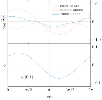
Refer to caption
Fig. 21: Upper panel: plots of the functions (of δψ𝛿𝜓\delta\psi) proportional to λ,λ2𝜆superscript𝜆2\lambda,\lambda^{2} and λ3superscript𝜆3\lambda^{3} in the slope of solution (159). Lower panel: plot of the slope ς3(λ)subscript𝜍3𝜆\varsigma_{3}(\lambda) as a function of δψ𝛿𝜓\delta\psi for λ=0.1𝜆0.1\lambda=0.1.
𝝋3(x)=π2\StrLen[\arglen]([xπ±𝝇3])2+nλnnϱ1n\StrLen[\arglen]([xπ±𝝇2])+n,mλnnλmmϱ2nm\StrLen[\arglen]([xπ±𝝇1])+n,m,pλnλmmλppϱ3nmp\StrLen[\arglen]([xπ])subscript𝝋3𝑥𝜋2\StrLendelimited-[]\arglensuperscriptabsentdelimited-[]plus-or-minus𝑥𝜋subscript𝝇32subscript𝑛subscript𝜆𝑛𝑛superscriptsubscriptbold-italic-ϱ1𝑛\StrLendelimited-[]\arglenabsentdelimited-[]plus-or-minus𝑥𝜋subscript𝝇2subscript𝑛𝑚subscript𝜆𝑛𝑛subscript𝜆𝑚𝑚superscriptsubscriptbold-italic-ϱ2𝑛𝑚\StrLendelimited-[]\arglenabsentdelimited-[]plus-or-minus𝑥𝜋subscript𝝇1subscript𝑛𝑚𝑝subscript𝜆𝑛subscript𝜆𝑚𝑚subscript𝜆𝑝𝑝superscriptsubscriptbold-italic-ϱ3𝑛𝑚𝑝\StrLendelimited-[]\arglenabsentdelimited-[]𝑥𝜋\displaystyle\bm{\varphi}_{3}(x)=\frac{\pi}{2}\!\StrLen{}[\arglen]\left(\vphantom{\left[\frac{x}{\sqrt{\pi}}\pm\bm{\varsigma}_{3}\right]^{\!\!\!2\,}}\!\!\sqrt{\vphantom{|}}\!\left[\frac{x}{\sqrt{\pi}}\pm\bm{\varsigma}_{3}\right]\!\right)^{\!\!\!2\,}\!+\sum_{n}\frac{\lambda_{n}}{n}\,\bm{\varrho}_{1}^{n}\!\StrLen{}[\arglen]\left(\vphantom{\left[\frac{x}{\sqrt{\pi}}\pm\bm{\varsigma}_{2}\right]^{\!\!\!2\,}}\!\!\sqrt{\vphantom{|}}\!\left[\frac{x}{\sqrt{\pi}}\pm\bm{\varsigma}_{2}\right]\!\right)\!+\sum_{n,\,m}\frac{\lambda_{n}}{\sqrt{n}}\frac{\lambda_{m}}{\sqrt{m}}\,\bm{\varrho}_{2}^{nm}\!\StrLen{}[\arglen]\left(\vphantom{\left[\frac{x}{\sqrt{\pi}}\pm\bm{\varsigma}_{1}\right]^{\!\!\!2\,}}\!\!\sqrt{\vphantom{|}}\!\left[\frac{x}{\sqrt{\pi}}\pm\bm{\varsigma}_{1}\right]\!\right)\!+\!\!\sum_{n,\,m,\,p}\!\!\lambda_{n}\frac{\lambda_{m}}{\sqrt{m}}\frac{\lambda_{p}}{\sqrt{p}}\,\bm{\varrho}_{3}^{nmp}\!\StrLen{}[\arglen]\left(\vphantom{\left[\frac{x}{\sqrt{\pi}}\right]^{\!\!\!2\,}}\!\!\sqrt{\vphantom{|}}\!\left[\frac{x}{\sqrt{\pi}}\right]\!\right) (160)
Refer to caption
Fig. 22: Graphical demonstration of the validity of the solutions to the phase resonance equation with a single mode and a non-zero initial phase, eq. (155). All these solutions involve the same λ=0.1𝜆0.1\lambda=0.1, but have different initial phases δψ𝛿𝜓\delta\psi.

This is the final and most important result of this article. While it is not easily usable in theoretical calculations, it could find applications in modelling resonances in new kludge waveforms, as this is not a feature currently implemented. We have provided a solution to the highest possible order of perturbation, which is important for meaningful numerical simulations. Furthermore, we have also provided solutions to simplified versions of this problem, which could be employed in various theoretical calculations regarding emris.

V Discussion and conclusions

In this paper we have described in Sections II and III the assumptions and conditions which form the basis of two different methods for analysis of resonances in emris. The two-timescale approach, described in van de Meent (2014) presumes that the functional dependence of the orbital characteristics can be expanded in power series of the mass-ratio and time from resonance. The instantaneous frequency model, as per Gair et al. (2012), relies on the instant values of the on-resonance frequencies as a basis for asymptotic analysis, and this is a more complicated function of the (rescaled) time.

After describing the basic approach, Section IV described in detail the solution to the frequency and phase resonance equations derived in the course of describing the instantaneous frequency approach. Some of these solutions were previously published in Gair et al. (2012). The difference between the frequency and phase resonances lies in the assumption about the phasing of the self-force. It is more natural that the phase will be determined by the instantaneous orbital phase (as in the phase treatment) than the orbital phase at some fiducial τ=0𝜏0\tau=0 (as in the frequency investigation). Fully-detailed self-force calculations would be needed to make an informed choice between the two, but it is likely that the phase approach is physically relevant for the resonance problem. The frequency resonance solutions exhibits interesting effects, in particular the “memory” effect on the slope of the graph, which would be interesting if it really occurred in any physical situation. Here we extended these results, by including higher-order terms and a generalised form of the solutions. We have derived solutions for the case of multiple oscillating modes, given by eq. (92). Working further, we have relaxed the assumption of a vanishing initial phase, and have presented the single-mode solution in eq. (112). Finally, combining these results we presented the complete frequency solution, eq. (121).

As mentioned above, the phase resonance equation is probably more relevant physically, as it describes the evolution of the phase coordinates near resonance, and its solutions can be related to the two-timescale method results. It is also interesting from a mathematical view point, since it is a second-order non-linear differential equation which can be approached using asymptotic methods. We extended the previously established sequence of results by deriving the third-order solution for the case of a single oscillating mode, eq. (133). We presented further toy models, discussed in detail in Appendices III and IV before demonstrating an order-by-order solution to the phase resonance equation with an arbitrary (possibly infinite) number of modes, eqs. (147), (150), and (249). Following this we presented the solution to the phase equation when the alternative initial assumption is relaxed: namely, the starting phase is allowed to vary. The first- and second-order solutions are given by eqs. (157) and (158). Finally, we have derived the solution in the most general case, allowing for an arbitrary (possibly infinite) number of modes, each with an individual initial phase. This solution was given in eq. (160). In the case that there is only a single mode, this calculation agrees with the result given in Gair et al. (2012), to leading order in the parameter λ𝜆\lambda, which is equivalent to the order of G1(𝐉)subscript𝐺1𝐉G_{1}(\mathbf{J}) in the two-timescale analysis.

Both the instantaneous frequency approach and the two-timescale analysis are valid treatments of the emri problem — though their foundational assumptions appear different, they both have the same computational complexity and arrive at equivalent conclusions. Previous work on the two-timescale method has only been presented to the lowest order in the mass ratio ϵitalic-ϵ\epsilon and the resonance flux change parameters {κ,λ}𝜅𝜆\{\kappa,\lambda\}. As has been discovered, in certain scenarios higher-order corrections in the latter can be more important than those to the former, hence it is vital to investigate the form of these corrections. This is what the current paper accomplishes.

Further work on solving the phase-resonance equation would use these equations in numerical waveform models. These could be utilised in implementing a computationally cheap approximate (kludge) model of emri waveforms which include resonance effects (Barack and Cutler, 2004; Babak et al., 2007). At the moment such models lack the necessary features to predict the change in frequency or phase on resonance, which is precisely what the results in this article offer. Therefore, this should be pursued in a future publication.

Electronic resources

Many of the results in this article are available in a Mathematica notebook, which can be found at:

http://resonances.deyanmihaylov.net/

Acknowledgements

Deyan P Mihaylov is supported by the stfc. He is thankful to Dr Christopher J Moore and to Alvin Chua for the engaging conversations about general relativity, cosmology, and gravitational wave astronomy.

References

Appendix A Kerr space-time

Since the background we consider in this article is exclusively the Kerr space-time, it is worth providing a summary of the metric for a rotating non-charged black hole. Alternatively, a charged and spinning black hole is described by the Kerr-Newman metric, while a non-rotating charged black hole solution is given by the Reissner-Nordstöm background. The Kerr metric, in Boyer-Lindquist coordinates (Boyer and Lindquist, 1982) (t,r,θ,ϕ)𝑡𝑟𝜃italic-ϕ(t,r,\theta,\phi), is given by:

and a=z/M𝑎subscript𝑧𝑀a=\mathcal{L}_{z}/M is the specific black hole spin parameter. This metric is singular at the points where θ={0,π}𝜃0𝜋\theta=\{0,\pi\}, however these are the usual coordinate singularities associated with the spherical polar system, remedied by the introduction of a second coordinate system. Further, we encounter coordinate singularities at the points where Δ(r)=0Δ𝑟0\Delta(r)=0, i.e., for values of the radial coordinate r±=M±M2+a2subscript𝑟plus-or-minusplus-or-minus𝑀superscript𝑀2superscript𝑎2r_{\pm}=M\pm\sqrt{M^{2}+a^{2}}. To demonstrate that these are merely coordinate singularities (and not an inherent curvature singularity of the metric), it is customary to make the change to Kerr coordinates (v,r,θ,χ)𝑣𝑟𝜃𝜒(v,r,\theta,\chi), given by (Visser, 2007):

dvd𝑣\displaystyle\mathop{}\!\mathrm{d}v =dt+r2+a2Δdr,absentd𝑡superscript𝑟2superscript𝑎2Δd𝑟\displaystyle=\mathop{}\!\mathrm{d}t+\frac{r^{2}+a^{2}}{\Delta}\,\mathop{}\!\mathrm{d}r\;, (162a)
dχd𝜒\displaystyle\mathop{}\!\mathrm{d}\chi =dϕ+aΔdr.absentditalic-ϕ𝑎Δd𝑟\displaystyle=\mathop{}\!\mathrm{d}\phi+\frac{a}{\Delta}\,\mathop{}\!\mathrm{d}r\;. (162b)
Refer to caption
Fig. 23: Visualisation of the Kerr space-time for a/M=0.95𝑎𝑀0.95a/M=0.95.

This shows that the metric could be analytically continued through the surface r±subscript𝑟plus-or-minusr_{\pm} to the region 0<r<r+0𝑟subscript𝑟0<r<r_{+}:

ds2=Δa2sin2θΣdv2+2dvdr2asin2θr2+a2ΔΣdvdχ2asin2θdχdr+(r2+a2)2Δa2sin2θΣsin2θdχ2+Σdθ2.dsuperscript𝑠2Δsuperscript𝑎2superscript2𝜃Σdsuperscript𝑣22d𝑣d𝑟2𝑎superscript2𝜃superscript𝑟2superscript𝑎2ΔΣd𝑣d𝜒2𝑎superscript2𝜃d𝜒d𝑟superscriptsuperscript𝑟2superscript𝑎22Δsuperscript𝑎2superscript2𝜃Σsuperscript2𝜃dsuperscript𝜒2Σdsuperscript𝜃2\begin{split}\mathop{}\!\mathrm{d}s^{2}=-\frac{\Delta-a^{2}\sin^{2}\theta}{\Sigma}\mathop{}\!\mathrm{d}v^{2}+2\mathop{}\!\mathrm{d}v\mathop{}\!\mathrm{d}r&-2a\sin^{2}\theta\,\frac{r^{2}+a^{2}-\Delta}{\Sigma}\mathop{}\!\mathrm{d}v\mathop{}\!\mathrm{d}\chi\\ &-2a\sin^{2}\theta\mathop{}\!\mathrm{d}\chi\mathop{}\!\mathrm{d}r+\frac{\left(r^{2}+a^{2}\right)^{2}-\Delta\,a^{2}\sin^{2}\theta}{\Sigma}\,\sin^{2}\theta\mathop{}\!\mathrm{d}\chi^{2}+\Sigma\mathop{}\!\mathrm{d}\theta^{2}.\end{split} (163)

The surface r=r+=M+M2a2𝑟subscript𝑟𝑀superscript𝑀2superscript𝑎2r=r_{+}=M+\sqrt{M^{2}-a^{2}} is a null hypersurface with normal 4-vector given by

ξa=(v)a+aa2+r+2(χ)a=(v)a+ΩKerr(χ)asuperscript𝜉𝑎superscript𝑣𝑎𝑎superscript𝑎2superscriptsubscript𝑟2superscript𝜒𝑎superscript𝑣𝑎subscriptΩKerrsuperscript𝜒𝑎\displaystyle\xi^{a}=\left(\frac{\partial}{\partial v}\right)^{\!\!\!a\,}+\frac{a}{a^{2}+r_{+}^{2}}\left(\frac{\partial}{\partial\chi}\right)^{\!\!\!a\,}=\left(\frac{\partial}{\partial v}\right)^{\!\!\!a\,}+\Omega_{\mathrm{Kerr}}\left(\frac{\partial}{\partial\chi}\right)^{\!\!\!a\,} (164)

and the region rr+𝑟subscript𝑟r\leq r_{+} is (part of) the black hole region. ΩsubscriptΩabsent\Omega_{\mathrm{}} is the angular velocity of the black hole with respect to an observer at infinity. There are several important surfaces in the Kerr space-time. Firstly, the curvature singularity r=0𝑟0r=0 is in fact a ring singularity, which can be explained as follows. A rotating black hole would not be spherically symmetric, as matter would bulge around the equator, the effect quantified by the spin parameter a𝑎a. Since a point singularity cannot support angular momentum, the lowest-dimensional shape required is a ring. This is evidenced by substituting tconst.𝑡𝑐𝑜𝑛𝑠𝑡t\equiv const., r=0𝑟0r=0, θ=π/2𝜃𝜋2\theta=\nicefrac{{\pi}}{{2}} (i.e., the singularity associated with Σ(r,θ)=0Σ𝑟𝜃0\Sigma(r,\theta)=0) in eq. (161a), obtaining ds2=a2dϕ2dsuperscript𝑠2superscript𝑎2dsuperscriptitalic-ϕ2\mathop{}\!\mathrm{d}s^{2}=a^{2}\mathop{}\!\mathrm{d}\phi^{2}, i.e., a ring of radius a𝑎a. Another important surface is the event horizon r+=M+M2a2subscript𝑟𝑀superscript𝑀2superscript𝑎2r_{+}=M+\sqrt{M^{2}-a^{2}}. To understand the final feature of interest, we consider the norm of the Killing vector field (/t)asuperscript𝑡𝑎(\partial/\partial t)^{a} in Boyer-Lindquist coordinates:

(t)2=Δa2sin2θΣ=1+2Mrr2+a2sin2θsuperscript𝑡2Δsuperscript𝑎2superscript2𝜃Σ12𝑀𝑟superscript𝑟2superscript𝑎2superscript2𝜃\displaystyle\left(\frac{\partial}{\partial t}\right)^{\!\!\!2\,}=-\frac{\Delta-a^{2}\sin^{2}\theta}{\Sigma}=-1+\frac{2Mr}{r^{2}+a^{2}\sin^{2}\theta} (165)

and notice that it is space-like ((/t)2<0superscript𝑡20(\partial/\partial t)^{2}<0) in the following region outside the event horizon r=r+𝑟subscript𝑟r=r_{+}:

M+M2a2<r<M+M2a2cos2θ.𝑀superscript𝑀2superscript𝑎2𝑟𝑀superscript𝑀2superscript𝑎2superscript2𝜃\displaystyle M+\sqrt{M^{2}-a^{2}}<r<M+\sqrt{M^{2}-a^{2}\cos^{2}\theta}. (166)

This region is called the ergosphere, and its outside surface is named the ergosurface, which intersects the event horizon at the poles θ=0,π𝜃0𝜋\theta=0,\pi. These surfaces are illustrated on the Kerr black-hole schematic on Fig. 23.

Appendix B Geodesic constants

One immediately notices that the Kerr metric does not depend on the time coordinate, t𝑡t, or the azimuthal angle, ϕitalic-ϕ\phi. Therefore, using the Euler-Lagrange equations, it can be shown that the conjugate momenta pμ=/q˙μsubscript𝑝𝜇superscript˙𝑞𝜇p_{\mu}=\partial\mathcal{L}/\partial\dot{q}^{\mu} associated to those coordinates are constant with respect to the affine parameter of the geodesic:

ddτ(q˙μ)=qμdpμdτ=qμ=0{ptconst.pϕconst.,formulae-sequenceformulae-sequencedd𝜏superscript˙𝑞𝜇superscript𝑞𝜇dsubscript𝑝𝜇d𝜏superscript𝑞𝜇0casessubscript𝑝𝑡𝑐𝑜𝑛𝑠𝑡otherwisesubscript𝑝italic-ϕ𝑐𝑜𝑛𝑠𝑡otherwise\displaystyle\frac{\mathop{}\!\mathrm{d}}{\mathop{}\!\mathrm{d}\tau}\!\left(\frac{\partial\mathcal{L}}{\partial\dot{q}^{\mu}}\right)=\frac{\partial\mathcal{L}}{\partial q^{\mu}}\quad\Leftrightarrow\quad\frac{\mathop{}\!\mathrm{d}p_{\mu}}{\mathop{}\!\mathrm{d}\tau}=\frac{\partial\mathcal{L}}{\partial q^{\mu}}=0\quad\Leftrightarrow\quad\begin{cases}p_{t}\equiv const.\\ p_{\phi}\equiv const.\;,\end{cases} (167)

where in general relativity, the Lagrangian is formally given by (q,q˙)=1/2gμνq˙μq˙ν𝑞˙𝑞12subscript𝑔𝜇𝜈superscript˙𝑞𝜇superscript˙𝑞𝜈\mathcal{L}(q,\dot{q})=\nicefrac{{1}}{{2}}\,g_{\mu\nu}\,\dot{q}^{\mu}\dot{q}^{\nu}. Thus we have identified 2 quantities which are constant along geodesics of the Kerr space-time. These are related to the energy of the orbit \mathcal{E}, and the axial component of the angular momentum zsubscript𝑧\mathcal{L}_{z}, respectively:

\displaystyle\mathcal{E} =pt=gtνq˙ν=Δa2sin2θΣt˙+asin2θr2+a2ΔΣϕ˙absentsubscript𝑝𝑡subscript𝑔𝑡𝜈superscript˙𝑞𝜈Δsuperscript𝑎2superscript2𝜃Σ˙𝑡𝑎superscript2𝜃superscript𝑟2superscript𝑎2ΔΣ˙italic-ϕ\displaystyle=-p_{t}=-g_{t\nu}\dot{q}^{\nu}=\dfrac{\Delta-a^{2}\sin^{2}\theta}{\Sigma}\,\dot{t}\,+\,a\sin^{2}\theta\,\dfrac{r^{2}+a^{2}-\Delta}{\Sigma}\,\dot{\phi} (168)
3subscript3\displaystyle\mathcal{L}_{3} =pϕ=gϕνq˙ν=asin2θr2+a2ΔΣt˙+(r2+a2)2Δa2sin2θΣsin2θϕ˙absentsubscript𝑝italic-ϕsubscript𝑔italic-ϕ𝜈superscript˙𝑞𝜈𝑎superscript2𝜃superscript𝑟2superscript𝑎2ΔΣ˙𝑡superscriptsuperscript𝑟2superscript𝑎22Δsuperscript𝑎2superscript2𝜃Σsuperscript2𝜃˙italic-ϕ\displaystyle=p_{\phi}=g_{\phi\nu}\dot{q}^{\nu}=-a\sin^{2}\theta\,\dfrac{r^{2}+a^{2}-\Delta}{\Sigma}\,\dot{t}\,+\,\dfrac{\left(r^{2}+a^{2}\right)^{2}-\Delta a^{2}\sin^{2}\theta}{\Sigma}\,\sin^{2}\theta\,\dot{\phi} (169)

For equatorial geodesics (θ=π/2𝜃𝜋2\theta=\nicefrac{{\pi}}{{2}}), these two constants are sufficient to uniquely determine a given geodesic. However, for general geodesics with 3 spatial degrees of freedom, we can identify a third constant of the motion, which is not associated with a linear symmetry of the background space-time.

Apart from the two Killing vectors associated with the Kerr metric, there exists a second-order Killing tensor for this background, Qμνsubscript𝑄𝜇𝜈Q_{\mu\nu}. This Killing tensor gives rise to another conserved quantity, which was originally discovered in 1968 as a consequence of the separable Hamilton-Jacobi equation. This quantity is called the Carter’s constant, and can be written as (Carter, 1968):

𝒬=Qμνpμpν=pθ2+cos2θ(a2(m22)+(zsinθ) 2).𝒬superscript𝑄𝜇𝜈subscript𝑝𝜇subscript𝑝𝜈superscriptsubscript𝑝𝜃2superscript2𝜃superscript𝑎2superscript𝑚2superscript2superscriptsubscript𝑧𝜃2\displaystyle\mathcal{Q}=Q^{\mu\nu}p_{\mu}p_{\nu}=p_{\theta}^{2}+\cos^{2}\theta\left(\!a^{2}\big{(}m^{2}-\mathcal{E}^{2}\big{)}+\left(\!\frac{\mathcal{L}_{z}}{\sin\theta}\!\right)^{\!\!\!\,2\,}\!\right). (170)

Appendix C Geodesics of the Kerr metric
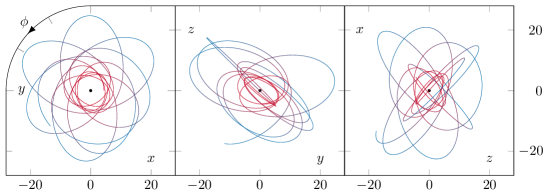
Refer to caption
(b)
Refer to caption
(c) (b) Evolution of the coordinates x𝑥x, y𝑦y and z𝑧z with physical time t𝑡t.
Refer to caption
(d) (c) A tridimensional view of the geodesic in Cartesian and cylindrical coordinate systems.
Fig. 24: A geodesics of the Kerr metric, and several projections, evolved for a period of 2×1052superscript1052\times 10^{5} s 5.56absent5.56\approx 5.56 hours. The orbit has eccentricity e=0.6𝑒0.6e=0.6 and semi-latus rectum 10M10𝑀10M, while the central black hole has mass M=106M𝑀superscript106subscript𝑀direct-productM=10^{6}M_{\odot} and spin 0.9M20.9superscript𝑀20.9M^{2}. All distances are in units of the black-hole mass M𝑀M. The angle of inclination is ι=45𝜄superscript45\iota=45^{\circ}, and the plane of inclination precesses.

The equatorial geodesics of the Kerr metric can be characterised by the constants \mathcal{E} and zsubscript𝑧\mathcal{L}_{z}, combined with the Hamiltonian, which is an additional integral of motion. General 3-dimensional geodesics, however, require the introduction of a further integral of motion, Carter’s constant, discussed in Appendix B. The equations of motion for a massless particle, as per Misner, Thorne, and Wheeler (1973), are given by

In the general case, these equation cannot be solved analytically to find a closed form of the shape of the geodesic. However, it is possible to integrate the equations numerically to find an approximate shape for a Kerr geodesic, and one possible solutions is shown in Fig. C. The Kerr geodesics are not closed, but rather fill the entire parameter space rmin<r<rmaxsubscript𝑟min𝑟subscript𝑟maxr_{\text{{min}}}<r<r_{\text{{max}}}, θmin<θ<θmaxsubscript𝜃min𝜃subscript𝜃max\theta_{\text{{min}}}<\theta<\theta_{\text{{max}}}, 0<ϕ<2π0italic-ϕ2𝜋0<\phi<2\pi (which has the shape of a torus) before returning to the starting (r,θ,ϕ)𝑟𝜃italic-ϕ(r,\theta,\phi). Moreover, the plane of inclination of the orbit is not stationary, but precesses around the black hole. In the case of a resonance, when two of the frequencies become commensurate, this configuration breaks down and the geodesic becomes a (simpler) closed curve around the black hole, defined only by 2 parameters.

Appendix D Fresnel integrals
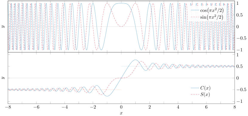
Refer to caption
Fig. 25: Upper panel: the integrands of the two Fresnel integrals, the functions cos(πx2/2)𝜋superscript𝑥22\cos\left(\pi x^{2}/2\right) and sin(πx2/2)𝜋superscript𝑥22\sin\left(\pi x^{2}/2\right), and the axis y=0𝑦0y=0 around which they oscillate. The frequency of oscillation increases with the absolute value of x𝑥x. Lower panel: numerical integration of the functions above gives the desired graphs of C(x)𝐶𝑥C(x) and S(x)𝑆𝑥S(x). They converge towards the line y=±1/2𝑦plus-or-minus12y=\pm\nicefrac{{1}}{{2}}.

In the course of solving the phase resonance equations, as well as in the presentation of the frequency resonance solution, we encounter integrals of trigonometric functions with quadratic arguments:

\bigintsss0xdysin(πy22)and\bigintsss0xdycos(πy22).superscriptsubscript\bigintsss0𝑥d𝑦𝜋superscript𝑦22andsuperscriptsubscript\bigintsss0𝑥d𝑦𝜋superscript𝑦22\displaystyle\bigintsss_{0}^{x}\!\!\!\mathop{}\!\mathrm{d}y\,\sin\!\left(\!\vphantom{\Bigg{[}\Bigg{]}}\frac{\pi y^{2}}{2}\!\right)\quad\text{and}\quad\bigintsss_{0}^{x}\!\!\!\mathop{}\!\mathrm{d}y\,\cos\!\left(\!\vphantom{\Bigg{[}\Bigg{]}}\frac{\pi y^{2}}{2}\!\right). (172)

These are known as the Fresnel integrals, after the French engineer and physicist Augustin-Jean Fresnel, who used them in optics. Here, we have adopted the notation where the argument of the integrand is premultiplied by π/2𝜋2\nicefrac{{\pi}}{{2}}. Please note that this definition is equivalent to the one used in Gair et al. (2010):

C(x)=2π0xdycos(y2).𝐶𝑥2𝜋superscriptsubscript0𝑥differential-d𝑦superscript𝑦2\displaystyle C(x)=\frac{\sqrt{2}}{\sqrt{\pi}}\int_{0}^{x}\mathop{}\!\mathrm{d}y\,\cos\!\left(y^{2}\right). (173)

These integrals are not directly solvable analytically, and therefore other methods for integration must be used. One approach to finding the two integrals in (172) is by expanding the integrands in converging Taylor series:

S(x)𝑆𝑥\displaystyle S(x) =\bigintsss0xdysin(πy22)=n=0(1)n(2n+1)!\bigintsss0xdy(πy22)2n+1=n=0(1)nπ2n+1(2n+1)!(4n+3) 22n+1x4n+3,absentsuperscriptsubscript\bigintsss0𝑥d𝑦𝜋superscript𝑦22superscriptsubscript𝑛0superscript1𝑛2𝑛1superscriptsubscript\bigintsss0𝑥d𝑦superscript𝜋superscript𝑦222𝑛1superscriptsubscript𝑛0superscript1𝑛superscript𝜋2𝑛12𝑛14𝑛3superscript22𝑛1superscript𝑥4𝑛3\displaystyle=\bigintsss_{0}^{x}\!\!\!\mathop{}\!\mathrm{d}y\sin\!\left(\!\vphantom{\Bigg{[}\Bigg{]}}\frac{\pi y^{2}}{2}\!\right)=\sum_{n=0}^{\infty}\frac{(-1)^{n}}{(2n+1)!}\bigintsss_{0}^{x}\!\!\!\mathop{}\!\mathrm{d}y\!\left(\!\vphantom{\Bigg{[}\Bigg{]}}\frac{\pi y^{2}}{2}\!\right)^{\!\!\!2n+1\,}\!\!\!\!=\sum_{n=0}^{\infty}\frac{(-1)^{n}\,\pi^{2n+1}}{(2n+1)!\,(4n+3)\,2^{2n+1}}\,x^{4n+3}, (174a)
C(x)𝐶𝑥\displaystyle C(x) =\bigintsss0xdycos(πy22)=n=0(1)n(2n)!\bigintsss0xdy(πy22)2n=n=0(1)nπ2n(2n)!(4n+1) 22nx4n+1.absentsuperscriptsubscript\bigintsss0𝑥d𝑦𝜋superscript𝑦22superscriptsubscript𝑛0superscript1𝑛2𝑛superscriptsubscript\bigintsss0𝑥d𝑦superscript𝜋superscript𝑦222𝑛superscriptsubscript𝑛0superscript1𝑛superscript𝜋2𝑛2𝑛4𝑛1superscript22𝑛superscript𝑥4𝑛1\displaystyle=\bigintsss_{0}^{x}\!\!\!\mathop{}\!\mathrm{d}y\cos\!\left(\!\vphantom{\Bigg{[}\Bigg{]}}\frac{\pi y^{2}}{2}\!\right)=\sum_{n=0}^{\infty}\frac{(-1)^{n}}{(2n)!}\bigintsss_{0}^{x}\!\!\!\mathop{}\!\mathrm{d}y\!\left(\!\vphantom{\Bigg{[}\Bigg{]}}\frac{\pi y^{2}}{2}\!\right)^{\!\!\!2n\,}\!\!\!\!=\sum_{n=0}^{\infty}\frac{(-1)^{n}\,\pi^{2n}}{(2n)!\,(4n+1)\,2^{2n}}\,x^{4n+1}. (174b)

Often, a symbol like the ones appearing on the left-hand sides of eqs. (174) are used in lieu of the actual series solutions. Hence, it is useful to know the first few terms of the series for each of the integrals:

The integrands and the integral functions are plotted in Fig. 25. We make note of several features: at x=0𝑥0x=0, S(x)𝑆𝑥S(x) starts flat, and progresses as x3similar-toabsentsuperscript𝑥3\sim x^{3}, while C(x)𝐶𝑥C(x) is linear. For positive or negative infinity, both functions tend to ±1/2plus-or-minus12\pm\nicefrac{{1}}{{2}}, and can be represented by an asymptotic expansion for large absolute values of x𝑥x:

S(x)=sgn(x)21πxcos(πx22)1π2x3sin(πx22)+3π3x5cos(πx22)+𝒪(x6),𝑆𝑥sgn𝑥21𝜋𝑥𝜋superscript𝑥221superscript𝜋2superscript𝑥3𝜋superscript𝑥223superscript𝜋3superscript𝑥5𝜋superscript𝑥22𝒪superscript𝑥6\displaystyle S(x)=\frac{\mathop{}\!\mathrm{sgn}(x)}{2}-\frac{1}{\pi x}\,\cos\!\Bigg{(}\!\frac{\pi x^{2}}{2}\!\Bigg{)}\!-\frac{1}{\pi^{2}x^{3}}\,\sin\!\Bigg{(}\!\frac{\pi x^{2}}{2}\!\Bigg{)}\!+\frac{3}{\pi^{3}x^{5}}\,\cos\!\Bigg{(}\!\frac{\pi x^{2}}{2}\!\Bigg{)}\!+\mathcal{O}\!\left(x^{-6}\right), (176a)
C(x)=sgn(x)2+1πxsin(πx22)1π2x3cos(πx22)3π3x5sin(πx22)+𝒪(x6).𝐶𝑥sgn𝑥21𝜋𝑥𝜋superscript𝑥221superscript𝜋2superscript𝑥3𝜋superscript𝑥223superscript𝜋3superscript𝑥5𝜋superscript𝑥22𝒪superscript𝑥6\displaystyle C(x)=\frac{\mathop{}\!\mathrm{sgn}(x)}{2}+\frac{1}{\pi x}\,\sin\!\Bigg{(}\!\frac{\pi x^{2}}{2}\!\Bigg{)}\!-\frac{1}{\pi^{2}x^{3}}\,\cos\!\Bigg{(}\!\frac{\pi x^{2}}{2}\!\Bigg{)}\!-\frac{3}{\pi^{3}x^{5}}\,\sin\!\Bigg{(}\!\frac{\pi x^{2}}{2}\!\Bigg{)}\!+\mathcal{O}\!\left(x^{-6}\right). (176b)

Appendix E Shorthand trigonometric notation

In eqs. (44) we define the following to make the discussion regarding the frequency mode equation easier to read: Sn(x)sin[n(ax+(1+b)x2)]subscript𝑆𝑛𝑥𝑛𝑎𝑥1𝑏superscript𝑥2\displaystyle S_{n}(x)\equiv\sin\!\left[n\Big{(}ax+\left(1+b\right)x^{2}\Big{)}\vphantom{\Big{(}\Big{)}^{\!\!\!2\,}}\!\right] (44a) Cn(x)cos[n(ax+(1+b)x2)].subscript𝐶𝑛𝑥𝑛𝑎𝑥1𝑏superscript𝑥2\displaystyle C_{n}(x)\equiv\cos\!\left[n\Big{(}ax+\left(1+b\right)x^{2}\Big{)}\vphantom{\Big{(}\Big{)}^{\!\!\!2\,}}\!\right]. (44b) for some arbitrary constants a𝑎a and b𝑏b.

Please note that these are different from the Fresnel integrals, denoted by the same letters, but without subscripts, discussed in Appendix D. These functions are plotted for several representative values of n𝑛n in Fig. 26. It is worth noting several identities which we make use of in the article, but do not derive explicitly. These follow directly from the product-to-sum formulae and the double angle formulae in trigonometry.
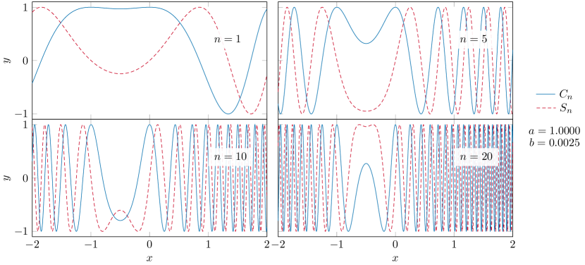
Refer to caption
Fig. 26: The functions Sn(x)subscript𝑆𝑛𝑥S_{n}(x) and Cn(x)subscript𝐶𝑛𝑥C_{n}(x) for several values of n𝑛n. As we can see, the functions oscillate (away from the region around x=0𝑥0x=0) more rapidly as n𝑛n increases. We have used values of a=1𝑎1a=1 and b=0.0025𝑏0.0025b=0.0025 for the constants.

We only consider positive values of the subscripts, with the following rules for negative values: Sn(x)=Sn(x)subscript𝑆𝑛𝑥subscript𝑆𝑛𝑥S_{-n}(x)=-S_{n}(x) and Cn(x)=Cn(x)subscript𝐶𝑛𝑥subscript𝐶𝑛𝑥C_{-n}(x)=C_{n}(x). It is important to note that these functions are linearly independent, i.e., they form a basis in functional space. This is most easily verified by considering the Wronskian for the sequence of functions

f0(x)=1,f1(x)=S1(x),f2(x)=C1(x),f3(x)=S2(x),f4(x)=C2(x) and so on.formulae-sequencesubscript𝑓0𝑥1formulae-sequencesubscript𝑓1𝑥subscript𝑆1𝑥formulae-sequencesubscript𝑓2𝑥subscript𝐶1𝑥formulae-sequencesubscript𝑓3𝑥subscript𝑆2𝑥subscript𝑓4𝑥subscript𝐶2𝑥 and so on.\displaystyle f_{0}(x)=1\;,\quad f_{1}(x)=S_{1}(x)\;,\quad f_{2}(x)=C_{1}(x)\;,\quad f_{3}(x)=S_{2}(x)\;,\quad f_{4}(x)=C_{2}(x)\;\text{ and so on.} (178)

For {f0(x),f1(x),f2(x)}subscript𝑓0𝑥subscript𝑓1𝑥subscript𝑓2𝑥\{f_{0}(x),f_{1}(x),f_{2}(x)\}, the Wronskian is (a+2(1+b)x)3superscript𝑎21𝑏𝑥3-(a+2(1+b)x)^{3}, while for the first 5 functions in the series, it is 72(a+2(1+b)x)1072superscript𝑎21𝑏𝑥1072(a+2(1+b)x)^{10}, both of which do not vanish in the general case. Since their Wronskian does not vanish, we can conclude that these functions are linearly independent over \{0}\0\mathbb{R}\,\backslash\{0\}:

W(f0,f1,f2,)(x)=det|f0(x)f1(x)f2(x)f3(x)f4(x)f0(x)f1(x)f2(x)f3(x)f4(x)f0′′(x)f1′′(x)f2′′(x)f3′′(x)f4′′(x)|0.𝑊subscript𝑓0subscript𝑓1subscript𝑓2𝑥matrixsubscript𝑓0𝑥subscript𝑓1𝑥subscript𝑓2𝑥subscript𝑓3𝑥subscript𝑓4𝑥missing-subexpressionsuperscriptsubscript𝑓0𝑥superscriptsubscript𝑓1𝑥superscriptsubscript𝑓2𝑥superscriptsubscript𝑓3𝑥superscriptsubscript𝑓4𝑥superscriptsubscript𝑓0′′𝑥superscriptsubscript𝑓1′′𝑥superscriptsubscript𝑓2′′𝑥superscriptsubscript𝑓3′′𝑥superscriptsubscript𝑓4′′𝑥missing-subexpressionmissing-subexpressionmissing-subexpressionmissing-subexpressionmissing-subexpression0\displaystyle W(f_{0},f_{1},f_{2},\ldots)(x)=\det\left|\begin{matrix}f_{0}(x)&f_{1}(x)&f_{2}(x)&f_{3}(x)&f_{4}(x)&\\[2.0pt] f_{0}^{\prime}(x)&f_{1}^{\prime}(x)&f_{2}^{\prime}(x)&f_{3}^{\prime}(x)&f_{4}^{\prime}(x)&\cdots\;\;\;\;\\[2.0pt] f_{0}^{\prime\prime}(x)&f_{1}^{\prime\prime}(x)&f_{2}^{\prime\prime}(x)&f_{3}^{\prime\prime}(x)&f_{4}^{\prime\prime}(x)&\\[2.0pt] &&\vdots&&&\ddots\;\;\;\;\\ \end{matrix}\right|\neq 0. (179)

It should be noted that these functions are not orthogonal. First, we show how to integrate a single factor of Sn(x)subscript𝑆𝑛𝑥S_{n}(x):

dxSn(x)superscriptsubscriptdifferential-d𝑥subscript𝑆𝑛𝑥\displaystyle\int_{-\infty}^{\infty}\mathop{}\!\mathrm{d}x\,S_{n}(x) =limL1L2+L1L2dxsin[π2(2n(1+b)π(x+a2(1+b)))2na24(1+b)]=absentsubscriptsubscript𝐿1subscript𝐿2superscriptsubscriptsubscript𝐿1subscript𝐿2differential-d𝑥𝜋2superscript2𝑛1𝑏𝜋𝑥𝑎21𝑏2𝑛superscript𝑎241𝑏absent\displaystyle=\lim_{\begin{subarray}{c}L_{1}\rightarrow-\infty\\ L_{2}\rightarrow+\infty\end{subarray}}\int_{L_{1}}^{L_{2}}\mathop{}\!\mathrm{d}x\,\sin\!\left[\frac{\pi}{2}\!\left(\!\sqrt{\frac{2n(1+b)}{\pi}}\left(\!x+\frac{a}{2(1+b)}\!\right)\!\right)^{2}\!\!-\frac{na^{2}}{4(1+b)}\right]=
=limL1L2+π2n(1+b)(cos[na24(1+b)](S(L2)S(L1))sin[na24(1+b)](C(L2)C(L1)))=absentsubscriptsubscript𝐿1subscript𝐿2𝜋2𝑛1𝑏𝑛superscript𝑎241𝑏𝑆subscript𝐿2𝑆subscript𝐿1𝑛superscript𝑎241𝑏𝐶subscript𝐿2𝐶subscript𝐿1absent\displaystyle=\lim_{\begin{subarray}{c}L_{1}\rightarrow-\infty\\ L_{2}\rightarrow+\infty\end{subarray}}\sqrt{\frac{\pi}{2n(1+b)}}\left(\cos\!\left[\vphantom{\Bigg{[}\Bigg{]}}\frac{na^{2}}{4(1+b)}\right]\!\big{(}S\left(L_{2}\right)-S\left(L_{1}\right)\!\big{)}-\sin\!\left[\vphantom{\Bigg{[}\Bigg{]}}\frac{na^{2}}{4(1+b)}\right]\!\big{(}C\left(L_{2}\right)-C\left(L_{1}\right)\!\big{)}\!\vphantom{\Bigg{[}\Bigg{]}^{\!\!\!2\,}}\right)=
=πn(1+b)cos[na24(1+b)+π4]absent𝜋𝑛1𝑏𝑛superscript𝑎241𝑏𝜋4\displaystyle=\sqrt{\frac{\pi}{n(1+b)}}\;\cos\!\left[\vphantom{\Bigg{[}\Bigg{]}}\frac{na^{2}}{4(1+b)}+\frac{\pi}{4}\right]

or similarly, a single factor of Cn(x)subscript𝐶𝑛𝑥C_{n}(x):

dxCn(x)superscriptsubscriptdifferential-d𝑥subscript𝐶𝑛𝑥\displaystyle\int_{-\infty}^{\infty}\mathop{}\!\mathrm{d}x\,C_{n}(x) =limL1L2+π2n(1+b)(cos[na24(1+b)](C(L2)C(L1))sin[na24(1+b)](S(L2)S(L1)))=absentsubscriptsubscript𝐿1subscript𝐿2𝜋2𝑛1𝑏𝑛superscript𝑎241𝑏𝐶subscript𝐿2𝐶subscript𝐿1𝑛superscript𝑎241𝑏𝑆subscript𝐿2𝑆subscript𝐿1absent\displaystyle=\lim_{\begin{subarray}{c}L_{1}\rightarrow-\infty\\ L_{2}\rightarrow+\infty\end{subarray}}\sqrt{\frac{\pi}{2n(1+b)}}\left(\cos\!\left[\vphantom{\Bigg{[}\Bigg{]}}\frac{na^{2}}{4(1+b)}\right]\!\big{(}C\left(L_{2}\right)-C\left(L_{1}\right)\!\big{)}-\sin\!\left[\vphantom{\Bigg{[}\Bigg{]}}\frac{na^{2}}{4(1+b)}\right]\!\big{(}S\left(L_{2}\right)-S\left(L_{1}\right)\!\big{)}\!\vphantom{\Bigg{[}\Bigg{]}^{\!\!\!2\,}}\right)=
=πn(1+b)sin[na24(1+b)+π4].absent𝜋𝑛1𝑏𝑛superscript𝑎241𝑏𝜋4\displaystyle=\sqrt{\frac{\pi}{n(1+b)}}\;\sin\!\left[\vphantom{\Bigg{[}\Bigg{]}}\frac{na^{2}}{4(1+b)}+\frac{\pi}{4}\right].

Here, S(x)𝑆𝑥S(x) and C(x)𝐶𝑥C(x) are the Fresnel integrals, whose properties and limits are discussed in Appendix D. Using these results, we can easily demonstrate that these functions do not form an orthogonal basis:

dxSn(x)Sm(x)=12dx(C(nm)(x)C(n+m)(x))==12π1+b(1|nm|sin[|nm|a24(1+b)+π4]1n+msin[(n+m)a24(1+b)+π4]),superscriptsubscriptdifferential-d𝑥subscript𝑆𝑛𝑥subscript𝑆𝑚𝑥12superscriptsubscriptdifferential-d𝑥subscript𝐶𝑛𝑚𝑥subscript𝐶𝑛𝑚𝑥12𝜋1𝑏1𝑛𝑚𝑛𝑚superscript𝑎241𝑏𝜋41𝑛𝑚𝑛𝑚superscript𝑎241𝑏𝜋4\displaystyle\begin{split}\int_{-\infty}^{\infty}\mathop{}\!\mathrm{d}x\,S_{n}(x)\,S_{m}(x)&=\frac{1}{2}\int_{-\infty}^{\infty}\mathop{}\!\mathrm{d}x\,\left(C_{\left(n-m\right)}(x)-C_{\left(n+m\right)}(x)\right)=\\ &=\frac{1}{2}\,\sqrt{\frac{\pi}{1+b}}\left(\!\vphantom{\Bigg{[}\Bigg{]}^{\!\!\!2\,}}\frac{1}{\sqrt{\left|n-m\right|}}\;\sin\!\left[\vphantom{\Bigg{[}\Bigg{]}}\frac{\left|n-m\right|a^{2}}{4(1+b)}+\frac{\pi}{4}\right]\!-\frac{1}{\sqrt{\vphantom{|}n+m}}\;\sin\!\left[\vphantom{\Bigg{[}\Bigg{]}}\frac{(n+m)a^{2}}{4(1+b)}+\frac{\pi}{4}\right]\!\right),\end{split} (180)

which does not vanish in general. Similar expressions can be obtained for integrals of Sn(x)Cm(x)subscript𝑆𝑛𝑥subscript𝐶𝑚𝑥S_{n}(x)\,C_{m}(x) and Cn(x)Cm(x)subscript𝐶𝑛𝑥subscript𝐶𝑚𝑥C_{n}(x)\,C_{m}(x).

Appendix F Solutions to the Frequency resonance equation

I Third-order solution

In the body of the article we derived in detail the solution to the single-mode frequency resonance equation (25) up to second order in the parameter κ𝜅\kappa. Here we extend the same solution method to derive the behaviour of ω(x)𝜔𝑥\omega(x) to 𝒪(κ3)𝒪superscript𝜅3\mathcal{O}\!\left(\kappa^{3}\right). Building onto our previous ansätze, eqs. (40) and (52), we suggest the third-order function

ω3(x)=asubscript𝜔3𝑥𝑎\displaystyle\omega_{3}(x)=a +(1+b3)x+c1S1(x)x+c2S2(x)x+c3S3(x)x+d1S1(x)x2+d2S2(x)x2+lln|x|.1subscript𝑏3𝑥subscript𝑐1subscript𝑆1𝑥𝑥subscript𝑐2subscript𝑆2𝑥𝑥subscript𝑐3subscript𝑆3𝑥𝑥subscript𝑑1subscript𝑆1𝑥superscript𝑥2subscript𝑑2subscript𝑆2𝑥superscript𝑥2𝑙𝑥\displaystyle+\left(1+b_{3}\right)x+c_{1}\frac{S_{1}(x)}{x}+c_{2}\frac{S_{2}(x)}{x}+c_{3}\frac{S_{3}(x)}{x}+d_{1}\frac{S_{1}(x)}{x^{2}}+d_{2}\frac{S_{2}(x)}{x^{2}}+l\ln\!|x|. (59)

where S3(x)=sin[3(ax+(1+b)x2)]subscript𝑆3𝑥3𝑎𝑥1𝑏superscript𝑥2S_{3}(x)=\sin\!\left[3\!\left(ax+(1+b)\,x^{2}\right)\right] and we assume that c3𝒪(κ3)similar-tosubscript𝑐3𝒪superscript𝜅3c_{3}\sim\mathcal{O}\!\left(\kappa^{3}\right), since it needs to match terms of 𝒪(κ3)𝒪superscript𝜅3\mathcal{O}\!\left(\kappa^{3}\right) in eq. (54). We substitute this proposed solution into our governing equation (25), and following rearrangement of both sides using familiar techniques, but this time keeping terms 𝒪(x1)𝒪superscript𝑥1\mathcal{O}\!\left(x^{-1}\right), we find

b+2(1+b3)c1C1(x)+4(1+b3)c2C2(x)+6(1+b3)c3C3(x)+lx+(c1a3+2(1+b3)d1)C1(x)x+(2c2a3+4(1+b3)d2)C2(x)x+(3c3a3+6(1+b3)d3)C3(x)x+𝒪(x2)κc12+(κκc128κc22)C1(x)+κc12C2(x)+(κc128+κc22)C3(x)κd121x+(κc1d12κd22)C1(x)x+κd12C2(x)x+κd22C3(x)x+𝒪(κ4).\displaystyle\begin{split}&b+2(1+b_{3})\,c_{1}\,C_{1}(x)+4(1+b_{3})\,c_{2}\,C_{2}(x)+6(1+b_{3})\,c_{3}\,C_{3}(x)+\frac{l}{x}\\ &\quad+\big{(}c_{1}a_{3}+2(1+b_{3})\,d_{1}\big{)}\frac{C_{1}(x)}{x}+\big{(}2c_{2}a_{3}+4(1+b_{3})\,d_{2}\big{)}\frac{C_{2}(x)}{x}+\big{(}3c_{3}a_{3}+6(1+b_{3})\,d_{3}\big{)}\frac{C_{3}(x)}{x}+\mathcal{O}\!\left(x^{-2}\right)\sim\\ &\quad\quad\sim-\frac{\kappa c_{1}}{2}+\left(\!\kappa-\frac{\kappa c_{1}^{2}}{8}-\frac{\kappa c_{2}}{2}\!\right)\!C_{1}(x)+\frac{\kappa c_{1}}{2}\,C_{2}(x)+\left(\!\frac{\kappa c_{1}^{2}}{8}+\frac{\kappa c_{2}}{2}\!\right)\!C_{3}(x)-\frac{\kappa d_{1}}{2}\,\frac{1}{x}+\\ &\quad\quad\quad\quad\left(\!-\frac{\kappa c_{1}d_{1}}{2}-\frac{\kappa d_{2}}{2}\!\right)\!\frac{C_{1}(x)}{x}+\frac{\kappa d_{1}}{2}\,\frac{C_{2}(x)}{x}+\frac{\kappa d_{2}}{2}\,\frac{C_{3}(x)}{x}+\mathcal{O}\!\left(\kappa^{4}\right).\end{split} (181)

Matching terms on both sides yields a system of coupled equations, which determines the coefficients:

bκc12,  2(1+b)c1κκc128κc22,  4(1+b)c2κc12,  6(1+b)c3κc128+κc22,lκd12,c1a3+2(1+b3)d1κc1d12κd22,  2c2a3+4(1+b3)d2κd12,  3c3a3+6(1+b3)d3κd22.formulae-sequencesimilar-to𝑏𝜅subscript𝑐12formulae-sequencesimilar-to21𝑏subscript𝑐1𝜅𝜅superscriptsubscript𝑐128𝜅subscript𝑐22formulae-sequencesimilar-to41𝑏subscript𝑐2𝜅subscript𝑐12formulae-sequencesimilar-to61𝑏subscript𝑐3𝜅superscriptsubscript𝑐128𝜅subscript𝑐22formulae-sequencesimilar-to𝑙𝜅subscript𝑑12formulae-sequencesimilar-tosubscript𝑐1subscript𝑎321subscript𝑏3subscript𝑑1𝜅subscript𝑐1subscript𝑑12𝜅subscript𝑑22formulae-sequencesimilar-to2subscript𝑐2subscript𝑎341subscript𝑏3subscript𝑑2𝜅subscript𝑑12similar-to3subscript𝑐3subscript𝑎361subscript𝑏3subscript𝑑3𝜅subscript𝑑22\displaystyle\begin{split}b\sim-\frac{\kappa c_{1}}{2}\;,\;\;2(1+b)\,c_{1}\sim\kappa-\frac{\kappa c_{1}^{2}}{8}-\frac{\kappa c_{2}}{2}\;,&\;\;4(1+b)\,c_{2}\sim\frac{\kappa c_{1}}{2}\;,\;\;6(1+b)\,c_{3}\sim\frac{\kappa c_{1}^{2}}{8}+\frac{\kappa c_{2}}{2}\;,\\[2.0pt] l\sim-\frac{\kappa d_{1}}{2}\;,\;\;c_{1}a_{3}+2(1+b_{3})\,d_{1}\sim-\frac{\kappa c_{1}d_{1}}{2}-\frac{\kappa d_{2}}{2}\;,&\;\;2c_{2}a_{3}+4(1+b_{3})\,d_{2}\sim\frac{\kappa d_{1}}{2}\;,\;\;3c_{3}a_{3}+6(1+b_{3})\,d_{3}\sim\frac{\kappa d_{2}}{2}.\end{split} (182)

These yield the following expressions for the undetermined coefficients of the anzats, eq. (59):

b14κ2,c112κ+332κ3,c2116κ2,c3196κ3,d12π16κ2±π64κ3,d22π64κ3,l±2π32κ3formulae-sequencesimilar-to𝑏14superscript𝜅2formulae-sequencesimilar-tosubscript𝑐112𝜅332superscript𝜅3formulae-sequencesimilar-tosubscript𝑐2116superscript𝜅2formulae-sequencesimilar-tosubscript𝑐3196superscript𝜅3formulae-sequencesimilar-tosubscript𝑑1plus-or-minusminus-or-plus2𝜋16superscript𝜅2𝜋64superscript𝜅3formulae-sequencesimilar-tosubscript𝑑2minus-or-plus2𝜋64superscript𝜅3similar-to𝑙plus-or-minus2𝜋32superscript𝜅3\displaystyle b\sim-\frac{1}{4}\,\kappa^{2}\,,\;\,c_{1}\sim\frac{1}{2}\,\kappa+\frac{3}{32}\,\kappa^{3}\,,\;\,c_{2}\sim\frac{1}{16}\,\kappa^{2}\,,\;\,c_{3}\sim\frac{1}{96}\,\kappa^{3}\,,\;\,d_{1}\sim\mp\frac{\sqrt{2\pi}}{16}\,\kappa^{2}\pm\frac{\sqrt{\pi}}{64}\,\kappa^{3}\,,\;\,d_{2}\sim\mp\frac{\sqrt{2\pi}}{64}\,\kappa^{3}\,,\;\,l\sim\pm\frac{\sqrt{2\pi}}{32}\,\kappa^{3}

and the solution to third order in κ𝜅\kappa can be written as

ω3(x)=a+(1κ24)x+κ121xsin[(±2π4κπ16κ2)x+(1κ24)x2]subscript𝜔3𝑥𝑎1superscript𝜅24𝑥𝜅121𝑥minus-or-plusplus-or-minus2𝜋4𝜅𝜋16superscript𝜅2𝑥1superscript𝜅24superscript𝑥2\displaystyle\omega_{3}(x)=a+\!\left(\!\vphantom{\Bigg{[}\Bigg{]}}1-\frac{\kappa^{2}}{4}\!\right)\!x+\kappa\,\frac{1}{2}\,\frac{1}{x}\,\sin\!\left[\vphantom{\Bigg{[}\Bigg{]}^{\!\!\!2\,}}\!\left(\!\pm\frac{\sqrt{2\pi}}{4}\,\kappa\mp\frac{\sqrt{\pi}}{16}\,\kappa^{2}\!\right)\!x+\!\Bigg{(}\!1-\frac{\kappa^{2}}{4}\!\Bigg{)}x^{2}\right]
+κ21161xsin[2((±2π4κ)x+x2)]+κ31x(332sin(x2)+196sin(3x2))superscript𝜅21161𝑥2plus-or-minus2𝜋4𝜅𝑥superscript𝑥2superscript𝜅31𝑥332superscript𝑥21963superscript𝑥2\displaystyle\quad\quad\quad\quad+\kappa^{2}\frac{1}{16}\,\frac{1}{x}\,\sin\!\left[\vphantom{\left[\Bigg{[}\Bigg{]}^{\!\!\!2\,}\right]^{\!\!\!2\,}}2\!\left(\!\!\vphantom{\Bigg{[}\Bigg{]}^{\!\!\!2\,}}\left(\!\pm\,\frac{\sqrt{2\pi}}{4}\,\kappa\!\right)\!x+x^{2}\!\right)\!\right]\!+\kappa^{3}\,\frac{1}{x}\!\left(\!\vphantom{\Bigg{[}\Bigg{]}}\frac{3}{32}\,\sin\!\left(x^{2}\right)+\frac{1}{96}\,\sin\!\left(3x^{2}\right)\!\right) (64)
κ22π161x2sin[(±2π4κ)x+x2]±κ3(π641x2sin(x2)2π641x2sin(2x2)+2π32ln|x|)plus-or-minusminus-or-plussuperscript𝜅22𝜋161superscript𝑥2plus-or-minus2𝜋4𝜅𝑥superscript𝑥2superscript𝜅3𝜋641superscript𝑥2superscript𝑥22𝜋641superscript𝑥22superscript𝑥22𝜋32𝑥\displaystyle\quad\quad\quad\quad\quad\quad\quad\quad\mp\kappa^{2}\frac{\sqrt{2\pi}}{16}\,\frac{1}{x^{2}}\,\sin\!\left[\vphantom{\Bigg{[}\Bigg{]}^{\!\!\!2\,}}\!\!\vphantom{\Bigg{[}\Bigg{]}^{\!\!\!2\,}}\left(\!\pm\,\frac{\sqrt{2\pi}}{4}\,\kappa\!\right)\!x+x^{2}\right]\!\pm\kappa^{3}\!\left(\!\vphantom{\Bigg{[}\Bigg{]}}\frac{\sqrt{\pi}}{64}\,\frac{1}{x^{2}}\,\sin\!\left(x^{2}\right)-\frac{\sqrt{2\pi}}{64}\,\frac{1}{x^{2}}\,\sin\!\left(2x^{2}\right)+\frac{\sqrt{2\pi}}{32}\,\ln\!|x|\!\right)

The value of the initial value parameter a3subscript𝑎3a_{3} is determined in the main body of the article.

II Frequency resonance equation with 𝐧𝟏𝐧1\mathbf{n\neq 1}

In Section IV.2 we solved the single-mode frequency resonance equation to obtain the solution (50). Instead of including the first oscillatory mode n=1𝑛1n=1, we now solve this equation for n=r𝑛𝑟n=r:

ω(x)=1+κrcos(rxω).superscript𝜔𝑥1subscript𝜅𝑟𝑟𝑥𝜔\displaystyle\omega^{\prime}(x)=1+\kappa_{r}\cos\left(rx\omega\right). (183)

We propose a version of the ansatz (40), with a modified oscillating term, reflecting the modified governing equation:

ωr(x)=a+(1+b)x+c1(r)sin(r(ax+(1+b)x2))x+𝒪(x1)=a+(1+b)x+c1(r)Sr(x)x+𝒪(x1).subscript𝜔𝑟𝑥𝑎1𝑏𝑥superscriptsubscript𝑐1𝑟𝑟𝑎𝑥1𝑏superscript𝑥2𝑥𝒪superscript𝑥1𝑎1𝑏𝑥superscriptsubscript𝑐1𝑟subscript𝑆𝑟𝑥𝑥𝒪superscript𝑥1\displaystyle\omega_{r}(x)=a+(1+b)\,x+c_{1}^{(r)}\,\frac{\sin\left(r\left(ax+(1+b)x^{2}\right)\right)}{x}+\mathcal{O}\!\left(x^{-1}\right)=a+(1+b)\,x+c_{1}^{(r)}\frac{S_{r}(x)}{x}+\mathcal{O}\!\left(x^{-1}\right). (184)

Upon substitution and carrying out the derivative and the Taylor expansion (valid since rκr1/rα1similar-to𝑟subscript𝜅𝑟1superscript𝑟𝛼1r\kappa_{r}\sim 1/r^{\alpha-1}), we obtain:

b+2r(1+b)c1(r)Cr(x)12rκrc1(r)+κrCr(x)+term involving C2r(x)similar-to𝑏2𝑟1𝑏superscriptsubscript𝑐1𝑟subscript𝐶𝑟𝑥12𝑟subscript𝜅𝑟superscriptsubscript𝑐1𝑟subscript𝜅𝑟subscript𝐶𝑟𝑥term involving C2r(x)\displaystyle b+2r(1+b)\,c_{1}^{(r)}C_{r}(x)\sim-\frac{1}{2}\,r\kappa_{r}c_{1}^{(r)}+\kappa_{r}C_{r}(x)+\,\text{{term involving} $C_{2r}(x)$} (185)

Matching the respective coefficients in the manner already familiar from above, we obtain the following expressions:

We have shown that b𝒪(κr2)similar-to𝑏𝒪superscriptsubscript𝜅𝑟2b\sim\mathcal{O}\!\left(\kappa_{r}^{2}\right) and c1(r)𝒪(κr/r)similar-tosuperscriptsubscript𝑐1𝑟𝒪subscript𝜅𝑟𝑟{c_{1}}^{(r)}\sim\mathcal{O}\!\left(\kappa_{r}/r\right) for the rthsuperscript𝑟thr^{\mathrm{th}} oscillating mode. Note that since (Drasco and Hughes, 2006) propose a value of α2greater-than-or-equivalent-to𝛼2\alpha\gtrsim 2, the series c1(n)superscriptsubscript𝑐1𝑛{c_{1}}^{(n)} converge, and our use of the Taylor expansion is valid.
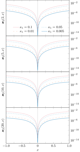
Refer to caption
Fig. 27: Graphical demonstration of the validity of solution (70) for different number of terms on the right-hand side. The coefficients {κn}subscript𝜅𝑛\{\kappa_{n}\} follow the power law κ1/n2.5subscript𝜅1superscript𝑛2.5\kappa_{1}/n^{2.5}. It is evident that the fractional errors scale with the value of the primary resonance modification κ1subscript𝜅1\kappa_{1}.
Refer to caption
Fig. 28: Graphical demonstration of the validity of solution (116) for different number of oscillating terms and for values of {δχn}𝛿subscript𝜒𝑛\{\delta\chi_{n}\} given by eq. (120). In all panels we have used κ1=0.1subscript𝜅10.1\kappa_{1}=0.1 with consecutive values given by κn=κ1/n2.5subscript𝜅𝑛subscript𝜅1superscript𝑛2.5\kappa_{n}=\kappa_{1}/n^{2.5}.

III Frequency resonance equation with two distinct modes

If we investigate the same equation with two distinct modes on the right-hand side, say n={r,s}𝑛𝑟𝑠n=\{r,s\}, with r<s𝑟𝑠r<s:

ω=1+κrcos(rxω)+κscos(sxω),superscript𝜔1subscript𝜅𝑟𝑟𝑥𝜔subscript𝜅𝑠𝑠𝑥𝜔\displaystyle\omega^{\prime}=1+\kappa_{r}\cos\left(rx\omega\right)+\kappa_{s}\cos\left(sx\omega\right), (187)

then the solution would include two leading-order terms associated with each of the two separate oscillating terms, with corrections at sub-leading order due to cross-terms between these. Specifically, we find c1(r)κr/2r(1+b)similar-tosuperscriptsubscript𝑐1𝑟subscript𝜅𝑟2𝑟1𝑏{c_{1}}^{(r)}\sim\kappa_{r}/2r(1+b) and c1(s)κs/2s(1+b)similar-tosuperscriptsubscript𝑐1𝑠subscript𝜅𝑠2𝑠1𝑏{c_{1}}^{(s)}\sim\kappa_{s}/2s(1+b), which implies that the coefficient b𝑏b is given by the expression

b12rκrc1(r)12sκsc1(s)κr2+κs24,similar-to𝑏12𝑟subscript𝜅𝑟superscriptsubscript𝑐1𝑟12𝑠subscript𝜅𝑠superscriptsubscript𝑐1𝑠similar-tosuperscriptsubscript𝜅𝑟2superscriptsubscript𝜅𝑠24\displaystyle b\sim-\frac{1}{2}\,r\,\kappa_{r}\,c_{1}^{(r)}-\frac{1}{2}\,s\,\kappa_{s}\,c_{1}^{(s)}\sim-\frac{\kappa_{r}^{2}+\kappa_{s}^{2}}{4}\,, (188)

and consequently

where each expression also includes sub-leading terms of order 𝒪(κrκs)𝒪subscript𝜅𝑟subscript𝜅𝑠\mathcal{O}\!\left(\kappa_{r}\kappa_{s}\right). This proves the important result that for the frequency equation with 2 distinct modes, all mixed terms (which depend on both κrsubscript𝜅𝑟\kappa_{r} and κssubscript𝜅𝑠\kappa_{s}) are of sub-leading order compared to the quadratic contributions originating from the individual modes as found earlier.

IV Frequency equation with a non-vanishing phase term

Let us consider the frequency equation with a single oscillating mode but with a non-vanishing phase term δχ𝛿𝜒\delta\chi:

ω(x)=1+κcos(xωδχ),superscript𝜔𝑥1𝜅𝑥𝜔𝛿𝜒\displaystyle\omega^{\prime}(x)=1+\kappa\cos\!\left(x\omega-\delta\chi\right), (93)

and let us expand the cosine term on the right-hand side to obtain the following differential equation:

ω(x)=1+κcos(δχ)cos(xω)+κsin(δχ)sin(xω).superscript𝜔𝑥1𝜅𝛿𝜒𝑥𝜔𝜅𝛿𝜒𝑥𝜔\displaystyle\omega^{\prime}(x)=1+\kappa\cos\!\left(\delta\chi\right)\cos\!\left(x\omega\right)+\kappa\sin\!\left(\delta\chi\right)\sin\!\left(x\omega\right). (190)

We may naively try the ansatz which previously proved suitable for the zero-phase version of the equation, given by eq. (40), however it will not work this time, as there will be unmatched terms left on the right-hand side. Instead, we suggest the following alternative ansatz, including an extra term proportional to C1(x)subscript𝐶1𝑥C_{1}(x)

ω1(x)=a+(1+b)x+c1S1(x)x+d1C1(x)x.subscript𝜔1𝑥𝑎1𝑏𝑥subscript𝑐1subscript𝑆1𝑥𝑥subscript𝑑1subscript𝐶1𝑥𝑥\displaystyle\omega_{1}(x)=a+\left(1+b\right)x+c_{1}\frac{S_{1}(x)}{x}+d_{1}\frac{C_{1}(x)}{x}. (191)

Upon differentiating and substituting on both sides of eq. (93), we obtain a more involved relation than before:

b+2(1+b)c1C1(x)2(1+b)d1S1(x)12κc1cos(δχ)12κd1sin(δχ)+κcos(δχ)C1(x)κsin(δχ)S1(x).similar-to𝑏21𝑏subscript𝑐1subscript𝐶1𝑥21𝑏subscript𝑑1subscript𝑆1𝑥12𝜅subscript𝑐1𝛿𝜒12𝜅subscript𝑑1𝛿𝜒𝜅𝛿𝜒subscript𝐶1𝑥𝜅𝛿𝜒subscript𝑆1𝑥\displaystyle b+2(1+b)c_{1}C_{1}(x)-2(1+b)d_{1}S_{1}(x)\sim-\frac{1}{2}\,\kappa\,c_{1}\cos\!\left(\delta\chi\right)-\frac{1}{2}\,\kappa\,d_{1}\sin\!\left(\delta\chi\right)+\kappa\cos\!\left(\delta\chi\right)C_{1}(x)-\kappa\sin\!\left(\delta\chi\right)S_{1}(x). (192)

Making the informed assumption that b𝒪(κ)similar-to𝑏𝒪𝜅b\sim\mathcal{O}\!\left(\kappa\right), we find the constants c1subscript𝑐1c_{1} and d1subscript𝑑1d_{1} by matching terms on both sides:

which is different from the previously found value of c1subscript𝑐1c_{1}. These yield the same value of the slope correction b𝑏b as before:

b12κc1cos(δχ)+12κd1sin(δχ)=κ22(cos2(δχ)+sin2(δχ))=κ22.similar-to𝑏12𝜅subscript𝑐1𝛿𝜒12𝜅subscript𝑑1𝛿𝜒superscript𝜅22superscript2𝛿𝜒superscript2𝛿𝜒superscript𝜅22\displaystyle b\sim-\frac{1}{2}\,\kappa\,c_{1}\cos\!\left(\delta\chi\right)+\frac{1}{2}\,\kappa\,d_{1}\sin\!\left(\delta\chi\right)=-\frac{\kappa^{2}}{2}\left(\cos^{2}\!\left(\delta\chi\right)+\sin^{2}\!\left(\delta\chi\right)\right)=-\frac{\kappa^{2}}{2}. (194)

If we substitute these into our proposed ansatz, we see that we recover the proposed alternative ansatz:

ω1(x)=a+x+κ21x(S1(x)cos(δχ)C1(x)sin(δχ))a+x+κ21xsin[ax+(1κ22)x2δχ],subscript𝜔1𝑥𝑎𝑥𝜅21𝑥subscript𝑆1𝑥𝛿𝜒subscript𝐶1𝑥𝛿𝜒𝑎𝑥𝜅21𝑥𝑎𝑥1superscript𝜅22superscript𝑥2𝛿𝜒\displaystyle\omega_{1}(x)=a+x+\frac{\kappa}{2}\,\frac{1}{x}\left(S_{1}(x)\cos\!\left(\delta\chi\right)-C_{1}(x)\sin\!\left(\delta\chi\right)\right)\equiv a+x+\frac{\kappa}{2}\,\frac{1}{x}\sin\!\left[\vphantom{\Bigg{[}\Bigg{]}^{\!\!\!2\,}}ax+\!\Bigg{(}\!1-\frac{\kappa^{2}}{2}\!\Bigg{)}x^{2}-\delta\chi\right], (195)

where the sine factor in the last term is identical to 𝒮1(x)subscript𝒮1𝑥\mathcal{S}_{1}(x), as defined in eq. (104a).

Appendix G Solutions to the phase resonance equation

In Section IV.3, we explain our algorithm for finding iterative solutions to the phase resonance equation, and present the solutions to third order in the parameter λ𝜆\lambda. However, we omit the details of finding these solutions, since these are often too tedious and irrelevant to our discussion. Here, we present these solutions in more detail. The zeroth-order equation (123) is straightforward to solve, by integrating both sides twice.

I Phase equation with a single mode and zero phase

Refer to caption
Fig. 29: Graphical comparison of the terms in the argument on the right-hand side of eq. (201). Evidently the term λρ1𝜆subscript𝜌1\lambda\,\rho_{1} stays close to 00 for all positive x𝑥x.
Fig. 30: Graphical comparison of the terms in the argument on the right-hand side of eq. (214). We can see that both terms, λρ1𝜆subscript𝜌1\lambda\,\rho_{1} and λ2ρ2superscript𝜆2subscript𝜌2\lambda^{2}\rho_{2}, are small compared to the other terms in the argument.

We source the first-order correction from the zeroth-order solution, and arrive at eq. (127). Integrating both sides between 00 and x𝑥x, making use of the Fresnel integrals, with initial condition ϕ(0)=0superscriptitalic-ϕ00\phi^{\prime}(0)=0, we find:

ϕ(1)(x)=λ0xdycos(y22)=πλC(xπ).superscriptsubscriptitalic-ϕ1𝑥𝜆superscriptsubscript0𝑥differential-d𝑦superscript𝑦22𝜋𝜆𝐶𝑥𝜋\displaystyle\phi_{(1)}^{\prime}(x)=\lambda\int_{0}^{x}\mathop{}\!\mathrm{d}y\,\cos\!\left(\vphantom{\Bigg{[}\Bigg{]}}\!\frac{y^{2}}{2}\!\right)=\sqrt{\pi}\,\lambda\,C\!\left(\!\frac{x}{\sqrt{\pi}}\!\right). (196)

Integrating once again, using the method of integration by parts, we obtain an initial form of the first-order correction:

ϕ(1)(x)=πλ0xdyC(yπ)=πλ[xC(xπ)1πsin(x22)].subscriptitalic-ϕ1𝑥𝜋𝜆superscriptsubscript0𝑥differential-d𝑦𝐶𝑦𝜋𝜋𝜆delimited-[]𝑥𝐶𝑥𝜋1𝜋superscript𝑥22\displaystyle\phi_{(1)}(x)=\sqrt{\pi}\,\lambda\!\int_{0}^{x}\!\mathop{}\!\mathrm{d}y\;C\!\left(\!\frac{y}{\sqrt{\pi}}\!\right)\!=\sqrt{\pi}\,\lambda\left[\vphantom{\Bigg{[}\Bigg{]}^{\!\!\!2\,}}x\,C\!\left(\!\frac{x}{\sqrt{\pi}}\!\right)\!-\frac{1}{\sqrt{\pi}}\,\sin\!\left(\vphantom{\Bigg{[}\Bigg{]}}\!\frac{x^{2}}{2}\!\right)\!\right]. (197)

While this is indeed a valid result, we prefer to re-arrange it in a form which is more useful for our tasks. If we look at the graph of this result for λ=0.1𝜆0.1\lambda=0.1 (Fig. 32), we can notice several features. First of all, since there are no constants dependant on λ𝜆\lambda in eq. (197), it vanishes at x=0𝑥0x=0. Furthermore, we immediately notice that the solution is a linear function which is modified by a decaying oscillating function. Therefore, we split the solution into two parts: a linear part, whose coefficient is a function of λ𝜆\lambda, and another part, a collection of periodic and quasi-periodic functions (trigonometric functions and Fresnel integrals) that collectively oscillates around ϕ=0italic-ϕ0\phi=0, and whose magnitude is small compared to the linear term. Since the graph is symmetric relative to the vertical axis, it is necessary to write down solutions for both cases x>0𝑥0x>0 and x<0𝑥0x<0. The Fresnel integrals oscillate around the value ±1/2plus-or-minus12\pm\nicefrac{{1}}{{2}} (instead of 0) for large ±xplus-or-minus𝑥\pm\,x, so we subtract this value from each of them in the rapidly oscillating terms. Finally, we note of an emerging pattern: the argument of the Fresnel integral is x/π𝑥𝜋x/\sqrt{\pi}, therefore we express the linear term and the remaining factors of x𝑥x in terms of this scaled variable. The upper sign is for positive x𝑥x, while the lower sign is for x<0𝑥0x<0.

ϕ(1)(x)=±π[12λ]\StrLen[\arglen]([xπ])missinglinear term+λ[π\StrLen[\arglen]([xπ])(C\StrLen[\arglen]([xπ])12)sin[π2\StrLen[\arglen]([xπ])2]]oscillating term proportional to λ.subscriptitalic-ϕ1𝑥subscriptplus-or-minus𝜋delimited-[]12𝜆\StrLendelimited-[]\arglenabsentdelimited-[]𝑥𝜋missinglinear termsubscript𝜆delimited-[]𝜋\StrLendelimited-[]\arglenabsentdelimited-[]𝑥𝜋minus-or-plus𝐶\StrLendelimited-[]\arglenabsentdelimited-[]𝑥𝜋12𝜋2\StrLendelimited-[]\arglensuperscriptabsentdelimited-[]𝑥𝜋2oscillating term proportional to λ\displaystyle\phi_{(1)}(x)=\underbrace{\pm\,\pi\!\left[\vphantom{\Bigg{[}\Bigg{]}}\frac{1}{2}\,\lambda\right]\!\!\StrLen{}[\arglen]\left(\vphantom{\left[\frac{x}{\sqrt{\pi}}\right]^{\!\!\!2\,}}\!\!\sqrt{\vphantom{|}}\!\left[\frac{x}{\sqrt{\pi}}\right]\!\right)missing}_{\text{{linear term}}}+\underbrace{\lambda\!\left[\vphantom{\Bigg{[}\Bigg{]}^{\!\!\!2\,}}\pi\!\StrLen{}[\arglen]\left(\vphantom{\left[\frac{x}{\sqrt{\pi}}\right]^{\!\!\!2\,}}\!\!\sqrt{\vphantom{|}}\!\left[\frac{x}{\sqrt{\pi}}\right]\!\right)\!\!\left(\!\vphantom{\left[\left[\frac{x}{\sqrt{\pi}}\right]^{\!\!\!2\,}\right]}C\!\StrLen{}[\arglen]\left(\vphantom{\left[\frac{x}{\sqrt{\pi}}\right]^{\!\!\!2\,}}\!\!\sqrt{\vphantom{|}}\!\left[\frac{x}{\sqrt{\pi}}\right]\!\right)\!\mp\frac{1}{2}\!\right)\!-\sin\!\left[\frac{\pi}{2}\!\StrLen{}[\arglen]\left(\vphantom{\left[\frac{x}{\sqrt{\pi}}\right]^{\!\!\!2\,}}\!\!\sqrt{\vphantom{|}}\!\left[\frac{x}{\sqrt{\pi}}\right]\!\right)^{\!\!\!2\,}\!\right]\!\right]}_{\text{{oscillating term proportional to $\lambda$}}}. (198)

We note that this result is strictly first order in the mode parameter λ𝜆\lambda. To construct the complete solution of the phase resonance equation to first order in λ𝜆\lambda, eq. (LABEL:eq:phase_solution_1), we combine eq. (198) with the zeroth-order function (124):

ϕ1(x)=π2\StrLen[\arglen]([xπ±12λ])2+λ[π\StrLen[\arglen]([xπ])(C\StrLen[\arglen]([xπ])12)sin[π2\StrLen[\arglen]([xπ])2]]+𝒪(λ2).subscriptitalic-ϕ1𝑥𝜋2\StrLendelimited-[]\arglensuperscriptabsentdelimited-[]plus-or-minus𝑥𝜋12𝜆2𝜆delimited-[]𝜋\StrLendelimited-[]\arglenabsentdelimited-[]𝑥𝜋minus-or-plus𝐶\StrLendelimited-[]\arglenabsentdelimited-[]𝑥𝜋12𝜋2\StrLendelimited-[]\arglensuperscriptabsentdelimited-[]𝑥𝜋2𝒪superscript𝜆2\displaystyle\phi_{1}(x)=\frac{\pi}{2}\!\StrLen{}[\arglen]\left(\vphantom{\left[\frac{x}{\sqrt{\pi}}\pm\frac{1}{2}\,\lambda\right]^{\!\!\!2\,}}\!\!\sqrt{\vphantom{|}}\!\left[\frac{x}{\sqrt{\pi}}\pm\frac{1}{2}\,\lambda\right]\!\right)^{\!\!\!2\,}\!+\lambda\!\left[\vphantom{\Bigg{[}\Bigg{]}^{\!\!\!2\,}}\pi\!\StrLen{}[\arglen]\left(\vphantom{\left[\frac{x}{\sqrt{\pi}}\right]^{\!\!\!2\,}}\!\!\sqrt{\vphantom{|}}\!\left[\frac{x}{\sqrt{\pi}}\right]\!\right)\!\!\left(\!\vphantom{\left[\left[\frac{x}{\sqrt{\pi}}\right]^{\!\!\!2\,}\right]}C\!\StrLen{}[\arglen]\left(\vphantom{\left[\frac{x}{\sqrt{\pi}}\right]^{\!\!\!2\,}}\!\!\sqrt{\vphantom{|}}\!\left[\frac{x}{\sqrt{\pi}}\right]\!\right)\!\mp\frac{1}{2}\!\right)\!-\sin\!\left[\frac{\pi}{2}\!\StrLen{}[\arglen]\left(\vphantom{\left[\frac{x}{\sqrt{\pi}}\right]^{\!\!\!2\,}}\!\!\sqrt{\vphantom{|}}\!\left[\frac{x}{\sqrt{\pi}}\right]\!\right)^{\!\!\!2\,}\!\right]\!\right]\!+\mathcal{O}\!\left(\lambda^{2}\right). (LABEL:eq:phase_solution_1)

We have combined the quadratic and linear terms into a single quadratic term, by implicitly adding the constant term (πλ2/8)𝜋superscript𝜆28(\pi\lambda^{2}/8), which is nevertheless ignored at linear order in the mode parameter, thus obtaining the form (LABEL:eq:phase_solution_1):

π2(xπ)2±π2λ(xπ)+𝒪(λ2)=π2(xπ±12λ)2+𝒪(λ2).plus-or-minus𝜋2superscript𝑥𝜋2𝜋2𝜆𝑥𝜋𝒪superscript𝜆2𝜋2superscriptplus-or-minus𝑥𝜋12𝜆2𝒪superscript𝜆2\displaystyle\frac{\pi}{2}\!\left(\!\frac{x}{\sqrt{\pi}}\!\right)^{\!\!\!2\,}\pm\frac{\pi}{2}\,\lambda\!\left(\!\frac{x}{\sqrt{\pi}}\!\right)\!+\mathcal{O}\!\left(\lambda^{2}\right)=\frac{\pi}{2}\!\left(\!\frac{x}{\sqrt{\pi}}\pm\frac{1}{2}\,\lambda\!\right)^{\!\!\!2\,}\!+\mathcal{O}\!\left(\lambda^{2}\right). (199)

Finally, we make note of the functional form of the oscillating term, which will be investigated in detail later together with the functions incurred at higher order (let X=x/π𝑋𝑥𝜋X=x/\!\sqrt{\pi} and see Appendix II for plots and discussion):

ρ1(X)=πX(C(X)12)sin(π2X2)subscript𝜌1𝑋𝜋𝑋minus-or-plus𝐶𝑋12𝜋2superscript𝑋2\displaystyle\rho_{1}(X)=\pi\,X\bigg{(}\!C\!\left(X\right)\mp\frac{1}{2}\!\bigg{)}\!-\sin\!\bigg{(}\!\frac{\pi}{2}\,X^{2}\!\bigg{)} (200)

The above result allows us to solve the equation at the next higher order, which is discussed below.

Finding the solution up to second order in λ𝜆\lambda involves substituting ϕ1(x)=ϕ0(x)+ϕ(1)(x)subscriptitalic-ϕ1𝑥subscriptitalic-ϕ0𝑥subscriptitalic-ϕ1𝑥\phi_{1}(x)=\phi_{0}(x)+\phi_{(1)}(x) on the right-hand side of the source equation (122), and solving for ϕ(2)(x)subscriptitalic-ϕ2𝑥\phi_{(2)}(x). Explicitly, eq. (129) is (we use the variant (197) of ϕ(1)(x)subscriptitalic-ϕ1𝑥\phi_{(1)}(x)):

ϕ(2)′′(x)=λcos[x22±π2λx+λ[πx(C\StrLen[\arglen]([xπ])12)sin(x22)]].superscriptsubscriptitalic-ϕ2′′𝑥𝜆plus-or-minussuperscript𝑥22𝜋2𝜆𝑥𝜆delimited-[]𝜋𝑥minus-or-plus𝐶\StrLendelimited-[]\arglenabsentdelimited-[]𝑥𝜋12superscript𝑥22\displaystyle\phi_{(2)}^{\prime\prime}(x)=\lambda\cos\!\left[\vphantom{\left[\Bigg{[}\Bigg{]}^{\!\!\!2\,}\right]^{\!\!\!2\,}}\frac{x^{2}}{2}\pm\frac{\sqrt{\pi}}{2}\,\lambda\,x+\lambda\!\left[\vphantom{\Bigg{[}\Bigg{]}^{\!\!\!2\,}}\sqrt{\pi}\,x\left(\!\vphantom{\left[\left[\frac{x}{\sqrt{\pi}}\right]^{\!\!\!2\,}\right]}C\!\StrLen{}[\arglen]\left(\vphantom{\left[\frac{x}{\sqrt{\pi}}\right]^{\!\!\!2\,}}\!\!\sqrt{\vphantom{|}}\!\left[\frac{x}{\sqrt{\pi}}\right]\!\right)\!\mp\frac{1}{2}\!\right)\!-\sin\!\left(\frac{x^{2}}{2}\right)\!\right]\!\right]. (201)

We write the last term in the argument of the cosine as λρ1(x/π)𝜆subscript𝜌1𝑥𝜋\lambda\,\rho_{1}\big{(}x/\!\sqrt{\pi}\big{)} and invoke our knowledge of trigonometric identities to write the right-hand side as:

ϕ(2)′′(x)=λcos(x22±π2λx)cos(λρ1(xπ))λsin(x22±π2λx)sin(λρ1(xπ))superscriptsubscriptitalic-ϕ2′′𝑥𝜆plus-or-minussuperscript𝑥22𝜋2𝜆𝑥𝜆subscript𝜌1𝑥𝜋𝜆plus-or-minussuperscript𝑥22𝜋2𝜆𝑥𝜆subscript𝜌1𝑥𝜋\displaystyle\phi_{(2)}^{\prime\prime}(x)=\lambda\cos\!\left(\vphantom{\Bigg{[}\Bigg{]}}\!\frac{x^{2}}{2}\pm\frac{\sqrt{\pi}}{2}\,\lambda\,x\!\right)\cos\!\left(\vphantom{\Bigg{[}\Bigg{]}}\!\lambda\,\rho_{1}\!\!\left(\!\frac{x}{\sqrt{\pi}}\!\right)\!\!\right)\!-\lambda\sin\!\left(\vphantom{\Bigg{[}\Bigg{]}}\!\frac{x^{2}}{2}\pm\frac{\sqrt{\pi}}{2}\,\lambda\,x\!\right)\sin\!\left(\vphantom{\Bigg{[}\Bigg{]}}\!\lambda\,\rho_{1}\!\!\left(\!\frac{x}{\sqrt{\pi}}\!\right)\!\!\right) (202)

The function ρ1(x/π)subscript𝜌1𝑥𝜋\rho_{1}\big{(}x/\!\sqrt{\pi}\big{)} oscillates around 0, and further, is pre-multiplied by the coefficient λ1much-less-than𝜆1\lambda\ll 1, hence we can assume that it is always small (compared to the quadratic and linear x𝑥x-terms, see Figure 30 for comparison of the relative magnitude of the terms), and use this fact to substitute the trigonometric functions involving ρ1subscript𝜌1\rho_{1} for Taylor series to leading order in λ𝜆\lambda. We ignore all terms of 𝒪(λ3)𝒪superscript𝜆3\mathcal{O}\!\left(\lambda^{3}\right) and higher, since they are not included at the current order.

ϕ(2)′′(x)=λcos(x22±π2λx)(1+𝒪(λ2))λsin(x22±π2λx)(λρ1(xπ)+𝒪(λ3))superscriptsubscriptitalic-ϕ2′′𝑥𝜆plus-or-minussuperscript𝑥22𝜋2𝜆𝑥1𝒪superscript𝜆2𝜆plus-or-minussuperscript𝑥22𝜋2𝜆𝑥𝜆subscript𝜌1𝑥𝜋𝒪superscript𝜆3\displaystyle\phi_{(2)}^{\prime\prime}(x)=\lambda\cos\!\left(\vphantom{\Bigg{[}\Bigg{]}}\!\frac{x^{2}}{2}\pm\frac{\sqrt{\pi}}{2}\,\lambda\,x\!\right)\!\left(1+\mathcal{O}\!\left(\lambda^{2}\right)\right)\!-\lambda\sin\!\left(\vphantom{\Bigg{[}\Bigg{]}}\!\frac{x^{2}}{2}\pm\frac{\sqrt{\pi}}{2}\,\lambda\,x\!\right)\!\left(\vphantom{\Bigg{[}\Bigg{]}}\!\lambda\,\rho_{1}\!\!\left(\!\frac{x}{\sqrt{\pi}}\!\right)\!+\mathcal{O}\!\left(\lambda^{3}\right)\!\right) (203)

We carry out the same procedure with the term multiplied by λ2superscript𝜆2\lambda^{2}, and neglect resulting terms proportional to λ3superscript𝜆3\lambda^{3}:

λ2sin(x22±π2λx)ρ1(xπ)=λ2sin(x22)ρ1(xπ)+𝒪(λ3).superscript𝜆2plus-or-minussuperscript𝑥22𝜋2𝜆𝑥subscript𝜌1𝑥𝜋superscript𝜆2superscript𝑥22subscript𝜌1𝑥𝜋𝒪superscript𝜆3\displaystyle\lambda^{2}\sin\!\left(\vphantom{\Bigg{[}\Bigg{]}}\!\frac{x^{2}}{2}\pm\frac{\sqrt{\pi}}{2}\,\lambda\,x\!\right)\rho_{1}\!\!\left(\!\frac{x}{\sqrt{\pi}}\!\right)=\lambda^{2}\sin\!\left(\vphantom{\Bigg{[}\Bigg{]}}\!\frac{x^{2}}{2}\!\right)\rho_{1}\!\!\left(\!\frac{x}{\sqrt{\pi}}\!\right)\!+\mathcal{O}\!\left(\lambda^{3}\right). (204)

Thus, we are left with the integral below, which can be easily performed using standard techniques, integration by parts and utilising the Fresnel integrals notation. We keep in mind to throw out terms of 𝒪(λ3)𝒪superscript𝜆3\mathcal{O}\!\left(\lambda^{3}\right) and higher.

ϕ(2)(x)superscriptsubscriptitalic-ϕ2𝑥\displaystyle\phi_{(2)}^{\prime}(x) =\bigintss0xdy[λcos(y22±π2λy)πλ2sin(y22)y(C(yπ)12)sin(y22)]=absentsuperscriptsubscript\bigintss0𝑥d𝑦delimited-[]𝜆plus-or-minussuperscript𝑦22𝜋2𝜆𝑦𝜋superscript𝜆2superscript𝑦22𝑦minus-or-plus𝐶𝑦𝜋12superscript𝑦22absent\displaystyle=\bigintss_{0}^{x}\!\!\!\!\mathop{}\!\mathrm{d}y\left[\vphantom{\Bigg{[}\Bigg{]}^{\!\!\!2\,}}\lambda\cos\!\left(\vphantom{\Bigg{[}\Bigg{]}}\!\frac{y^{2}}{2}\pm\frac{\sqrt{\pi}}{2}\,\lambda\,y\!\right)\!-\sqrt{\pi}\,\lambda^{2}\sin\!\left(\vphantom{\Bigg{[}\Bigg{]}}\!\frac{y^{2}}{2}\!\right)y\left(\vphantom{\Bigg{[}\Bigg{]}}\!C\!\left(\!\frac{y}{\sqrt{\pi}}\!\right)\!\mp\frac{1}{2}\!\right)\!-\sin\!\left(\vphantom{\Bigg{[}\Bigg{]}}\!\frac{y^{2}}{2}\!\right)\right]= (205)
=πλ[C(xπ±λ2)C(λ2)]+πλ2[cos(x22)C(xπ)12C(2xπ)12cos(x22)±12].absent𝜋𝜆delimited-[]minus-or-plus𝐶plus-or-minus𝑥𝜋𝜆2𝐶𝜆2𝜋superscript𝜆2delimited-[]plus-or-minusminus-or-plussuperscript𝑥22𝐶𝑥𝜋12𝐶2𝑥𝜋12superscript𝑥2212\displaystyle=\sqrt{\pi}\,\lambda\Bigg{[}C\!\left(\!\frac{x}{\sqrt{\pi}}\pm\frac{\lambda}{2}\!\right)\!\mp C\!\left(\frac{\lambda}{2}\right)\!\Bigg{]}\!+\sqrt{\pi}\,\lambda^{2}\!\left[\vphantom{\Bigg{[}\Bigg{]}^{\!\!\!2\,}}\cos\!\left(\vphantom{\Bigg{[}\Bigg{]}}\!\frac{x^{2}}{2}\!\right)C\!\left(\!\frac{x}{\sqrt{\pi}}\!\right)\!-\frac{1}{\sqrt{2}}\,C\!\left(\!\frac{\sqrt{2}\,x}{\sqrt{\pi}}\!\right)\!\mp\frac{1}{2}\cos\!\left(\vphantom{\Bigg{[}\Bigg{]}}\!\frac{x^{2}}{2}\!\right)\!\pm\frac{1}{2}\right]. (206)

We need to integrate this further once again, keeping track of the initial condition, ϕ(0)=0italic-ϕ00\phi(0)=0. We obtain the following expression for the correction, where again the upper sign is valid for x>0𝑥0x>0 and the lower for x<0𝑥0x<0:

ϕ(2)(x)=πλ[xC(xπ±λ2)1πsin[π2\StrLen[\arglen]([xπ±12λ])2]C(λ2)x]+πλ2[π2C2(xπ)π2C(xπ)±π2C(xπ±λ2)12xC(2xπ)+12πsin(x2)±x2]subscriptitalic-ϕ2𝑥𝜋𝜆delimited-[]minus-or-plus𝑥𝐶plus-or-minus𝑥𝜋𝜆21𝜋𝜋2\StrLendelimited-[]\arglensuperscriptabsentdelimited-[]plus-or-minus𝑥𝜋12𝜆2𝐶𝜆2𝑥𝜋superscript𝜆2delimited-[]plus-or-minusplus-or-minusminus-or-plus𝜋2superscript𝐶2𝑥𝜋𝜋2𝐶𝑥𝜋𝜋2𝐶plus-or-minus𝑥𝜋𝜆212𝑥𝐶2𝑥𝜋12𝜋superscript𝑥2𝑥2\displaystyle\begin{split}\phi_{(2)}(x)&=\sqrt{\pi}\,\lambda\!\left[\vphantom{\left[\Bigg{[}\Bigg{]}^{\!\!\!2\,}\right]^{\!\!\!2\,}}x\,C\!\left(\!\frac{x}{\sqrt{\pi}}\pm\frac{\lambda}{2}\!\right)-\frac{1}{\sqrt{\pi}}\,\sin\!\left[\frac{\pi}{2}\!\StrLen{}[\arglen]\left(\vphantom{\left[\frac{x}{\sqrt{\pi}}\pm\frac{1}{2}\,\lambda\right]^{\!\!\!2\,}}\!\!\sqrt{\vphantom{|}}\!\left[\frac{x}{\sqrt{\pi}}\pm\frac{1}{2}\,\lambda\right]\!\right)^{\!\!\!2\,}\!\right]\!\mp C\!\left(\frac{\lambda}{2}\right)x\right]\\ &+\sqrt{\pi}\,\lambda^{2}\!\left[\vphantom{\left[\Bigg{[}\Bigg{]}^{\!\!\!2\,}\right]^{\!\!\!2\,}}\frac{\sqrt{\pi}}{2}\,C^{2}\!\left(\!\frac{x}{\sqrt{\pi}}\!\right)\mp\frac{\sqrt{\pi}}{2}\,C\!\left(\!\frac{x}{\sqrt{\pi}}\!\right)\!\pm\frac{\sqrt{\pi}}{2}\,C\!\left(\!\frac{x}{\sqrt{\pi}}\pm\frac{\lambda}{2}\!\right)\!-\frac{1}{\sqrt{2}}\,x\,C\!\left(\!\frac{\sqrt{2}\,x}{\sqrt{\pi}}\!\right)+\frac{1}{2\sqrt{\pi}}\,\sin\!\left(x^{2}\right)\pm\frac{x}{2}\right]\end{split} (207)

We have obtained an expression which gives the correction to the quadratic term to second order in λ𝜆\lambda, which can be seen plotted in Figure 32. Again, we seek to express this in a modified form where the linear term is explicit, and all the oscillating terms are grouped by order of the parameter λ𝜆\lambda, which allows for better understanding of the solution.
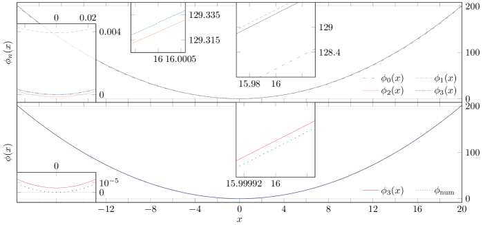
Refer to caption
Fig. 31: Upper panel: All four solutions (124) – (133) represented on the same plot. Evidently, they are all very close to each other, and cannot be easily distinguished in this manner. The three insets show features of the plot. At the origin, the solutions vanish up to a small deviation of magnitude comparable with the next respective order. Upon zooming in closer, one can distinguish the graphs from each other. Lower panel: Visual comparison of the highest-order solution, ϕ3(x)subscriptitalic-ϕ3𝑥\phi_{3}(x), and the numerical solution of the phase resonance equation. In all calculations and simulations we have used value of λ=0.1𝜆0.1\lambda=0.1.
ϕ(2)(x)=±π[λ2λC(λ2)+2122λ2]xlinear term+π8λ2constant+λ[π\StrLen[\arglen]([xπ±12λ])(C\StrLen[\arglen]([xπ±12λ])12)sin[π2\StrLen[\arglen]([xπ±12λ])2]]oscillating term proportional to λ+λ2[π2(C\StrLen[\arglen]([xπ])12)2π2\StrLen2[\arglen](2[xπ])(C\StrLen2[\arglen](2[xπ])12)+12sin[π2\StrLen2[\arglen](2[xπ])2]]oscillating term proportional to λ2.subscriptitalic-ϕ2𝑥subscriptplus-or-minus𝜋delimited-[]𝜆2𝜆𝐶𝜆22122superscript𝜆2𝑥linear termsubscript𝜋8superscript𝜆2constantsubscript𝜆delimited-[]𝜋\StrLendelimited-[]\arglenabsentdelimited-[]plus-or-minus𝑥𝜋12𝜆minus-or-plus𝐶\StrLendelimited-[]\arglenabsentdelimited-[]plus-or-minus𝑥𝜋12𝜆12𝜋2\StrLendelimited-[]\arglensuperscriptabsentdelimited-[]plus-or-minus𝑥𝜋12𝜆2oscillating term proportional to λsubscriptsuperscript𝜆2delimited-[]𝜋2superscriptminus-or-plus𝐶\StrLendelimited-[]\arglenabsentdelimited-[]𝑥𝜋122𝜋2\StrLen2delimited-[]\arglen2delimited-[]𝑥𝜋minus-or-plus𝐶\StrLen2delimited-[]\arglen2delimited-[]𝑥𝜋1212𝜋2\StrLen2delimited-[]\arglensuperscript2delimited-[]𝑥𝜋2oscillating term proportional to λ2\displaystyle\begin{split}\phi_{(2)}(x)&=\underbrace{\pm\sqrt{\pi}\left[\frac{\lambda}{2}-\lambda\,C\!\left(\frac{\lambda}{2}\right)+\frac{\sqrt{2}-1}{2\sqrt{2}}\,\lambda^{2}\right]x}_{\text{{linear term}}}\;\;+\underbrace{\vphantom{\Bigg{(}\Bigg{)}}\frac{\pi}{8}\,\lambda^{2}}_{\text{{constant}}}\\[5.0pt] &\phantom{\quad\quad}+\underbrace{\lambda\!\left[\vphantom{\left[\Bigg{[}\Bigg{]}^{\!\!\!2\,}\right]^{\!\!\!2\,}}\pi\!\StrLen{}[\arglen]\left(\vphantom{\left[\frac{x}{\sqrt{\pi}}\pm\frac{1}{2}\,\lambda\right]^{\!\!\!2\,}}\!\!\sqrt{\vphantom{|}}\!\left[\frac{x}{\sqrt{\pi}}\pm\frac{1}{2}\,\lambda\right]\!\right)\!\!\left(\vphantom{\Bigg{[}\Bigg{]}^{\!\!\!2\,}}\!C\!\StrLen{}[\arglen]\left(\vphantom{\left[\frac{x}{\sqrt{\pi}}\pm\frac{1}{2}\,\lambda\right]^{\!\!\!2\,}}\!\!\sqrt{\vphantom{|}}\!\left[\frac{x}{\sqrt{\pi}}\pm\frac{1}{2}\,\lambda\right]\!\right)\!\mp\frac{1}{2}\!\right)\!-\sin\!\left[\frac{\pi}{2}\!\StrLen{}[\arglen]\left(\vphantom{\left[\frac{x}{\sqrt{\pi}}\pm\frac{1}{2}\,\lambda\right]^{\!\!\!2\,}}\!\!\sqrt{\vphantom{|}}\!\left[\frac{x}{\sqrt{\pi}}\pm\frac{1}{2}\,\lambda\right]\!\right)^{\!\!\!2\,}\!\right]\!\right]}_{\text{{oscillating term proportional to $\lambda$}}}\\[5.0pt] &\phantom{\quad\quad\quad\quad}+\underbrace{\lambda^{2}\!\left[\vphantom{\left[\Bigg{[}\Bigg{]}^{\!\!\!2\,}\right]^{\!\!\!2\,}}\frac{\pi}{2}\!\left(\!\vphantom{\left[\left[\frac{x}{\sqrt{\pi}}\right]^{\!\!\!2\,}\right]}C\!\StrLen{}[\arglen]\left(\vphantom{\left[\frac{x}{\sqrt{\pi}}\right]^{\!\!\!2\,}}\!\!\sqrt{\vphantom{|}}\!\left[\frac{x}{\sqrt{\pi}}\right]\!\right)\!\mp\frac{1}{2}\!\right)^{\!\!\!2\,}\!-\frac{\pi}{2}\!\StrLen{2}[\arglen]\left(\vphantom{\left[\frac{x}{\sqrt{\pi}}\right]^{\!\!\!2\,}}\!\!\sqrt{\vphantom{|}2}\!\left[\frac{x}{\sqrt{\pi}}\right]\!\right)\!\!\left(\!\vphantom{\left[\left[\frac{x}{\sqrt{\pi}}2\right]^{\!\!\!2\,}\right]^{\!\!\!2\,}}C\!\StrLen{2}[\arglen]\left(\vphantom{\left[\frac{x}{\sqrt{\pi}}\right]^{\!\!\!2\,}}\!\!\sqrt{\vphantom{|}2}\!\left[\frac{x}{\sqrt{\pi}}\right]\!\right)\!\mp\frac{1}{2}\!\right)\!+\frac{1}{2}\,\sin\!\left[\frac{\pi}{2}\!\StrLen{2}[\arglen]\left(\vphantom{\left[\frac{x}{\sqrt{\pi}}\right]^{\!\!\!2\,}}\!\!\sqrt{\vphantom{|}2}\!\left[\frac{x}{\sqrt{\pi}}\right]\!\right)^{\!\!\!2\,}\!\right]\!\right]}_{\text{{oscillating term proportional to $\lambda^{2}$}}}.\end{split} (208)

We note that some of these terms, if expanded, would be 𝒪(λ3)𝒪superscript𝜆3\mathcal{O}\!\left(\lambda^{3}\right) or higher, but we leave them in for presentational purposes. We simplify the coefficient of the linear term (the slope of the derivative ϕ2(x)superscriptsubscriptitalic-ϕ2𝑥\phi_{2}^{\;\prime}(x)), by writing the Fresnel integral in power series, and retaining only its linear term (the next higher-order term is of fifth order):

λ2λC(λ2)+2122λ2=λ2λ22+2122λ2+𝒪(λ6)12λ24λ2.𝜆2𝜆𝐶𝜆22122superscript𝜆2𝜆2superscript𝜆222122superscript𝜆2𝒪superscript𝜆612𝜆24superscript𝜆2\displaystyle\frac{\lambda}{2}-\lambda\,C\!\left(\frac{\lambda}{2}\right)+\frac{\sqrt{2}-1}{2\sqrt{2}}\,\lambda^{2}=\frac{\lambda}{2}-\frac{\lambda^{2}}{2}+\frac{\sqrt{2}-1}{2\sqrt{2}}\,\lambda^{2}+\mathcal{O}\!\left(\lambda^{6}\right)\approx\frac{1}{2}\,\lambda-\frac{\sqrt{2}}{4}\,\lambda^{2}. (209)

When we combine this with the zeroth-order function ϕ0(x)=x2/2subscriptitalic-ϕ0𝑥superscript𝑥22\phi_{0}(x)=x^{2}/2, we find the complete second-order solution, given by eq. (131). Specifically, we can complete the square with the quadratic, linear, and constant terms, to obtain

x22±π[12λ24λ2]x+π8λ2=π2\StrLen[\arglen]([xπ±[12λ24λ2]])2+𝒪(λ3).plus-or-minussuperscript𝑥22𝜋delimited-[]12𝜆24superscript𝜆2𝑥𝜋8superscript𝜆2𝜋2\StrLendelimited-[]\arglensuperscriptabsentdelimited-[]plus-or-minus𝑥𝜋delimited-[]12𝜆24superscript𝜆22𝒪superscript𝜆3\displaystyle\frac{x^{2}}{2}\pm\sqrt{\pi}\left[\frac{1}{2}\,\lambda-\frac{\sqrt{2}}{4}\,\lambda^{2}\right]x+\frac{\pi}{8}\,\lambda^{2}=\frac{\pi}{2}\!\StrLen{}[\arglen]\left(\vphantom{\left[\frac{x}{\sqrt{\pi}}\pm\!\left[\frac{1}{2}\,\lambda-\frac{\sqrt{2}}{4}\,\lambda^{2}\right]\right]^{\!\!\!2\,}}\!\!\sqrt{\vphantom{|}}\!\left[\frac{x}{\sqrt{\pi}}\pm\!\left[\frac{1}{2}\,\lambda-\frac{\sqrt{2}}{4}\,\lambda^{2}\right]\right]\!\right)^{\!\!\!2\,}\!+\mathcal{O}\!\left(\lambda^{3}\right). (210)

In deriving this solution, we have used familiar integration techniques, and the definition of the Fresnel integrals, however it is useful to quote one of the “tricks” for the benefit of the reader who wishes to replicate these results:

\bigintsss±f(λ)x/π±f(λ)dycos(π2y2)=C(xπ±f(λ))C(f(λ)).superscriptsubscript\bigintsssplus-or-minus𝑓𝜆plus-or-minus𝑥𝜋𝑓𝜆d𝑦𝜋2superscript𝑦2minus-or-plus𝐶plus-or-minus𝑥𝜋𝑓𝜆𝐶𝑓𝜆\displaystyle\bigintsss_{\pm f(\lambda)}^{x/\!\sqrt{\pi}\,\pm f(\lambda)}\!\!\!\!\!\!\!\!\mathop{}\!\mathrm{d}y\cos\!\bigg{(}\!\frac{\pi}{2}\,y^{2}\!\bigg{)}\!=C\!\left(\!\frac{x}{\sqrt{\pi}}\pm f(\lambda)\!\right)\!\mp C\big{(}f(\lambda)\big{)}. (211)

It is important to pay attention to the two oscillating terms in eq. (208): the first one, has the same functional form as the oscillating term in eq. (198), and can in fact be related to ρ1(X)subscript𝜌1𝑋\rho_{1}(X) in the following way:

oscillating term proportional to λ=ρ1(xπ±12λ).oscillating term proportional to λsubscript𝜌1plus-or-minus𝑥𝜋12𝜆\displaystyle\text{\footnotesize{{oscillating term proportional to $\lambda$}}}=\rho_{1}\!\!\left(\!\frac{x}{\sqrt{\pi}}\pm\frac{1}{2}\,\lambda\!\right). (212)

The second oscillating term has not been encountered before, and will be investigated in detail in Appendix II:

ρ2(X)=π2(C(X)12) 2π2(2X)(C(2X)12)+12sin[π2(2X) 2].subscript𝜌2𝑋𝜋2superscriptminus-or-plus𝐶𝑋122𝜋22𝑋minus-or-plus𝐶2𝑋1212𝜋2superscript2𝑋2\displaystyle\rho_{2}(X)=\frac{\pi}{2}\bigg{(}\!C\!\left(X\right)\mp\frac{1}{2}\bigg{)}^{\!\!\!\,2\,}\!-\frac{\pi}{2}\!\left(\!\sqrt{2}\,X\right)\!\left(\!C\!\left(\sqrt{2}\,X\right)\!\mp\frac{1}{2}\right)\!+\frac{1}{2}\,\sin\!\left[\frac{\pi}{2}\!\left(\!\sqrt{2}\,X\right)^{\!\!\!\,2\,}\right]. (213)

As we can see, the second-order solution ϕ2(x)=ϕ0(x)+ϕ(2)(x)subscriptitalic-ϕ2𝑥subscriptitalic-ϕ0𝑥subscriptitalic-ϕ2𝑥\phi_{2}(x)=\phi_{0}(x)+\phi_{(2)}(x) is already heavily involved. Extending the results in (Gair et al., 2010), we use this function to source the third-order solution, see below for details.

Refer to caption
Fig. 32: Graphical comparison of the three corrections ϕ(1)(x)subscriptitalic-ϕ1𝑥\phi_{(1)}(x), ϕ(2)(x)subscriptitalic-ϕ2𝑥\phi_{(2)}(x), and ϕ(3)(x)subscriptitalic-ϕ3𝑥\phi_{(3)}(x) for λ=0.1𝜆0.1\lambda=0.1. At the origin, ϕ(1)(0)=0subscriptitalic-ϕ100\phi_{(1)}(0)=0 as it does not involve a constant term, while ϕ(2)(0)subscriptitalic-ϕ20\phi_{(2)}(0) and ϕ(3)(0)subscriptitalic-ϕ30\phi_{(3)}(0) do not vanish, but rather obey the condition to 𝒪(λ3)𝒪superscript𝜆3\mathcal{O}\!\left(\lambda^{3}\right) and 𝒪(λ4)𝒪superscript𝜆4\mathcal{O}\!\left(\lambda^{4}\right), respectively, which is within their errors: |ϕ(2)(0)|<λ3subscriptitalic-ϕ20superscript𝜆3|\phi_{(2)}(0)|<\lambda^{3} and |ϕ(3)(0)|<λ4subscriptitalic-ϕ30superscript𝜆4|\phi_{(3)}(0)|<\lambda^{4}.

Substituting the expression (133) for ϕ2(x)subscriptitalic-ϕ2𝑥\phi_{2}(x) into eq. (132) gives the equation we need to solve at third order:

ϕ(3)′′(x)superscriptsubscriptitalic-ϕ3′′𝑥\displaystyle\phi_{(3)}^{\;\prime\prime}(x) =λcos[x22±π(12λ24λ2)x+π8λ2+λρ1(xπ±12λ)+λ2ρ2(xπ)],absent𝜆plus-or-minussuperscript𝑥22𝜋12𝜆24superscript𝜆2𝑥𝜋8superscript𝜆2𝜆subscript𝜌1plus-or-minus𝑥𝜋12𝜆superscript𝜆2subscript𝜌2𝑥𝜋\displaystyle=\lambda\,\cos\!\left[\vphantom{\Bigg{[}\Bigg{]}^{\!\!\!2\,}}\frac{x^{2}}{2}\pm\sqrt{\pi}\left(\!\frac{1}{2}\,\lambda-\frac{\sqrt{2}}{4}\,\lambda^{2}\!\right)\!x+\frac{\pi}{8}\,\lambda^{2}+\lambda\,\rho_{1}\!\!\left(\!\frac{x}{\sqrt{\pi}}\pm\frac{1}{2}\,\lambda\!\right)+\lambda^{2}\,\rho_{2}\!\!\left(\!\frac{x}{\sqrt{\pi}}\!\right)\!\right], (214)
where ρ1(xπ±12λ)=π\StrLen[\arglen]([xπ±12λ])(C\StrLen[\arglen]([xπ±12λ])12)sin[π2\StrLen[\arglen]([xπ±12λ])2]subscript𝜌1plus-or-minus𝑥𝜋12𝜆𝜋\StrLendelimited-[]\arglenabsentdelimited-[]plus-or-minus𝑥𝜋12𝜆minus-or-plus𝐶\StrLendelimited-[]\arglenabsentdelimited-[]plus-or-minus𝑥𝜋12𝜆12𝜋2\StrLendelimited-[]\arglensuperscriptabsentdelimited-[]plus-or-minus𝑥𝜋12𝜆2\displaystyle\quad\rho_{1}\!\!\left(\!\frac{x}{\sqrt{\pi}}\pm\frac{1}{2}\,\lambda\!\right)=\pi\!\StrLen{}[\arglen]\left(\vphantom{\left[\frac{x}{\sqrt{\pi}}\pm\frac{1}{2}\,\lambda\right]^{\!\!\!2\,}}\!\!\sqrt{\vphantom{|}}\!\left[\frac{x}{\sqrt{\pi}}\pm\frac{1}{2}\,\lambda\right]\!\right)\!\!\left(\vphantom{\Bigg{[}\Bigg{]}^{\!\!\!2\,}}\!C\!\StrLen{}[\arglen]\left(\vphantom{\left[\frac{x}{\sqrt{\pi}}\pm\frac{1}{2}\,\lambda\right]^{\!\!\!2\,}}\!\!\sqrt{\vphantom{|}}\!\left[\frac{x}{\sqrt{\pi}}\pm\frac{1}{2}\,\lambda\right]\!\right)\!\mp\frac{1}{2}\!\right)\!-\sin\!\left[\frac{\pi}{2}\!\StrLen{}[\arglen]\left(\vphantom{\left[\frac{x}{\sqrt{\pi}}\pm\frac{1}{2}\,\lambda\right]^{\!\!\!2\,}}\!\!\sqrt{\vphantom{|}}\!\left[\frac{x}{\sqrt{\pi}}\pm\frac{1}{2}\,\lambda\right]\!\right)^{\!\!\!2\,}\!\right] (215)
and ρ2(xπ)=π2(C\StrLen[\arglen]([xπ])12)2π2\StrLen2[\arglen](2[xπ])(C\StrLen2[\arglen](2[xπ])12)+12sin[π2\StrLen2[\arglen](2[xπ])2].subscript𝜌2𝑥𝜋𝜋2superscriptminus-or-plus𝐶\StrLendelimited-[]\arglenabsentdelimited-[]𝑥𝜋122𝜋2\StrLen2delimited-[]\arglen2delimited-[]𝑥𝜋minus-or-plus𝐶\StrLen2delimited-[]\arglen2delimited-[]𝑥𝜋1212𝜋2\StrLen2delimited-[]\arglensuperscript2delimited-[]𝑥𝜋2\displaystyle\quad\rho_{2}\!\!\left(\!\frac{x}{\sqrt{\pi}}\!\right)=\frac{\pi}{2}\!\left(\!\vphantom{\left[\left[\frac{x}{\sqrt{\pi}}\right]^{\!\!\!2\,}\right]}C\!\StrLen{}[\arglen]\left(\vphantom{\left[\frac{x}{\sqrt{\pi}}\right]^{\!\!\!2\,}}\!\!\sqrt{\vphantom{|}}\!\left[\frac{x}{\sqrt{\pi}}\right]\!\right)\!\mp\frac{1}{2}\!\right)^{\!\!\!2\,}\!-\frac{\pi}{2}\!\StrLen{2}[\arglen]\left(\vphantom{\left[\frac{x}{\sqrt{\pi}}\right]^{\!\!\!2\,}}\!\!\sqrt{\vphantom{|}2}\!\left[\frac{x}{\sqrt{\pi}}\right]\!\right)\!\!\left(\!\vphantom{\left[\left[\frac{x}{\sqrt{\pi}}2\right]^{\!\!\!2\,}\right]^{\!\!\!2\,}}C\!\StrLen{2}[\arglen]\left(\vphantom{\left[\frac{x}{\sqrt{\pi}}\right]^{\!\!\!2\,}}\!\!\sqrt{\vphantom{|}2}\!\left[\frac{x}{\sqrt{\pi}}\right]\!\right)\!\mp\frac{1}{2}\!\right)\!+\frac{1}{2}\,\sin\!\left[\frac{\pi}{2}\!\StrLen{2}[\arglen]\left(\vphantom{\left[\frac{x}{\sqrt{\pi}}\right]^{\!\!\!2\,}}\!\!\sqrt{\vphantom{|}2}\!\left[\frac{x}{\sqrt{\pi}}\right]\!\right)^{\!\!\!2\,}\!\right]. (216)

It is important to realise that λρ1()𝜆subscript𝜌1\lambda\,\rho_{1}(\bullet) and λ2ρ2()superscript𝜆2subscript𝜌2\lambda^{2}\rho_{2}(\bullet) are small in magnitude compared to the other terms, as is obvious when these are plotted on the same graph, see Figure 30. Hence we can treat these as a perturbation to the rest of the argument. This becomes obvious when the functions are plotted on the same graph, see Figure 30. This prompts us to expand the cosine term using the sum-to-product formulae, and expand the terms containing the perturbation:

λcos[x22±π(12λ24λ2)x+π8λ2+λρ1(xπ±12λ)+λ2ρ2(xπ)]=𝜆plus-or-minussuperscript𝑥22𝜋12𝜆24superscript𝜆2𝑥𝜋8superscript𝜆2𝜆subscript𝜌1plus-or-minus𝑥𝜋12𝜆superscript𝜆2subscript𝜌2𝑥𝜋absent\displaystyle\lambda\,\cos\!\left[\vphantom{\Bigg{[}\Bigg{]}^{\!\!\!2\,}}\frac{x^{2}}{2}\pm\sqrt{\pi}\left(\!\frac{1}{2}\,\lambda-\frac{\sqrt{2}}{4}\,\lambda^{2}\!\right)\!x+\frac{\pi}{8}\,\lambda^{2}+\lambda\,\rho_{1}\!\!\left(\!\frac{x}{\sqrt{\pi}}\pm\frac{1}{2}\,\lambda\!\right)+\lambda^{2}\,\rho_{2}\!\!\left(\!\frac{x}{\sqrt{\pi}}\!\right)\!\right]= (217)
=λcos[x22±π(12λ24λ2)x+π8λ2]×cos(λρ1(xπ±12λ)+λ2ρ2(xπ))λsin[x22±π(12λ24λ2)x+π8λ2]×sin(λρ1(xπ±12λ)+λ2ρ2(xπ))=\displaystyle\begin{split}&=\lambda\,\cos\!\left[\vphantom{\Bigg{[}\Bigg{]}^{\!\!\!2\,}}\frac{x^{2}}{2}\pm\sqrt{\pi}\left(\!\frac{1}{2}\,\lambda-\frac{\sqrt{2}}{4}\,\lambda^{2}\!\right)\!x+\frac{\pi}{8}\,\lambda^{2}\right]\!\times\cos\!\left(\vphantom{\Bigg{[}\Bigg{]}}\!\lambda\,\rho_{1}\!\!\left(\!\frac{x}{\sqrt{\pi}}\pm\frac{1}{2}\,\lambda\!\right)+\lambda^{2}\,\rho_{2}\!\!\left(\!\frac{x}{\sqrt{\pi}}\!\right)\!\right)\\ &\quad\quad\quad\quad\quad\quad\quad\quad\quad\quad-\lambda\,\sin\!\left[\vphantom{\Bigg{[}\Bigg{]}^{\!\!\!2\,}}\frac{x^{2}}{2}\pm\sqrt{\pi}\left(\!\frac{1}{2}\,\lambda-\frac{\sqrt{2}}{4}\,\lambda^{2}\!\right)\!x+\frac{\pi}{8}\,\lambda^{2}\right]\!\times\sin\!\left(\vphantom{\Bigg{[}\Bigg{]}}\!\lambda\,\rho_{1}\!\!\left(\!\frac{x}{\sqrt{\pi}}\pm\frac{1}{2}\,\lambda\!\right)+\lambda^{2}\,\rho_{2}\!\!\left(\!\frac{x}{\sqrt{\pi}}\!\right)\!\right)=\end{split} (218)
=λcos[x22±π(12λ24λ2)x+π8λ2]λ2sin(x22±π2λx)ρ1(xπ±12λ)12λ3(cos(x22)ρ12(xπ±12λ)+2sin(x22)ρ2(xπ))+𝒪(λ4).absent𝜆plus-or-minussuperscript𝑥22𝜋12𝜆24superscript𝜆2𝑥𝜋8superscript𝜆2superscript𝜆2plus-or-minussuperscript𝑥22𝜋2𝜆𝑥subscript𝜌1plus-or-minus𝑥𝜋12𝜆12superscript𝜆3superscript𝑥22superscriptsubscript𝜌12plus-or-minus𝑥𝜋12𝜆2superscript𝑥22subscript𝜌2𝑥𝜋𝒪superscript𝜆4\displaystyle\begin{split}&=\lambda\,\cos\!\left[\vphantom{\Bigg{[}\Bigg{]}^{\!\!\!2\,}}\frac{x^{2}}{2}\pm\sqrt{\pi}\left(\!\frac{1}{2}\,\lambda-\frac{\sqrt{2}}{4}\,\lambda^{2}\!\right)\!x+\frac{\pi}{8}\,\lambda^{2}\right]\!-\lambda^{2}\sin\!\left(\vphantom{\Bigg{[}\Bigg{]}}\!\frac{x^{2}}{2}\pm\frac{\sqrt{\pi}}{2}\,\lambda\,x\!\right)\rho_{1}\!\!\left(\!\frac{x}{\sqrt{\pi}}\pm\frac{1}{2}\,\lambda\!\right)\\ &\quad\quad\quad\quad\quad\quad\quad\quad\quad\quad-\frac{1}{2}\,\lambda^{3}\left(\vphantom{\Bigg{[}\Bigg{]}}\!\cos\!\left(\vphantom{\Bigg{[}\Bigg{]}}\!\frac{x^{2}}{2}\!\right)\rho_{1}^{2}\!\!\left(\!\frac{x}{\sqrt{\pi}}\pm\frac{1}{2}\,\lambda\!\right)+2\,\sin\!\left(\vphantom{\Bigg{[}\Bigg{]}}\!\frac{x^{2}}{2}\!\right)\rho_{2}\!\!\left(\!\frac{x}{\sqrt{\pi}}\!\right)\!\right)\!+\mathcal{O}\!\left(\lambda^{4}\right).\end{split} (219)

We have combined both third-order terms together, since it makes the integration more straightforward. Integrating the expression (219), subject to the boundary condition ϕ(0)=0superscriptitalic-ϕ00\phi^{\prime}(0)=0 gives the derivative of the third-order correction:

ϕ(3)(x)superscriptsubscriptitalic-ϕ3𝑥\displaystyle\phi_{(3)}^{\prime}(x) =πλ[C(xπ±[12λ24λ2])C(12λ24λ2)]absent𝜋𝜆delimited-[]minus-or-plus𝐶plus-or-minus𝑥𝜋delimited-[]12𝜆24superscript𝜆2𝐶12𝜆24superscript𝜆2\displaystyle=\sqrt{\pi}\,\lambda\!\left[\vphantom{\left[\Bigg{[}\Bigg{]}^{\!\!\!2\,}\right]^{\!\!\!2\,}}C\!\left(\vphantom{\Bigg{[}\Bigg{]}^{\!\!\!2\,}}\!\frac{x}{\sqrt{\pi}}\pm\!\left[\frac{1}{2}\,\lambda-\frac{\sqrt{2}}{4}\,\lambda^{2}\right]\!\right)\!\mp C\!\left(\!\frac{1}{2}\,\lambda-\frac{\sqrt{2}}{4}\,\lambda^{2}\!\right)\!\right]
+πλ2[cos(x22±π2λx)C(xπ±λ2)12cos(x22±π2λx)\displaystyle+\sqrt{\pi}\,\lambda^{2}\left[\vphantom{\Bigg{[}\Bigg{]}^{\!\!\!2\,}}\cos\!\left(\vphantom{\Bigg{[}\Bigg{]}}\!\frac{x^{2}}{2}\pm\frac{\sqrt{\pi}}{2}\,\lambda\,x\!\right)C\!\left(\!\frac{x}{\sqrt{\pi}}\pm\frac{\lambda}{2}\!\right)\!\mp\frac{1}{2}\,\cos\!\left(\vphantom{\Bigg{[}\Bigg{]}}\!\frac{x^{2}}{2}\pm\frac{\sqrt{\pi}}{2}\,\lambda\,x\!\right)\right.
12C(2xπ±λ2)±12C(λ2)C(λ2)±12]\displaystyle\quad\quad\quad\quad\quad\quad\quad\quad\left.\vphantom{\Bigg{[}\Bigg{]}^{\!\!\!2\,}}-\frac{1}{\sqrt{2}}\,C\!\left(\!\frac{\sqrt{2}\,x}{\sqrt{\pi}}\pm\frac{\lambda}{\sqrt{2}}\!\right)\!\pm\frac{1}{\sqrt{2}}\,C\!\left(\!\frac{\lambda}{\sqrt{2}}\!\right)\!\mp C\!\left(\frac{\lambda}{2}\right)\!\pm\frac{1}{2}\right] (220)
πλ3[π2xsin(x22)[C 2(xπ)C(xπ)+14]38C(xπ)338C(3xπ)\displaystyle-\sqrt{\pi}\,\lambda^{3}\left[\vphantom{\left[\Bigg{[}\Bigg{]}^{\!\!\!2\,}\right]^{\!\!\!2\,}}\frac{\sqrt{\pi}}{2}\,x\,\sin\!\left(\vphantom{\Bigg{[}\Bigg{]}}\!\frac{x^{2}}{2}\!\right)\!\left[\vphantom{\Bigg{[}\Bigg{]}}C^{\,2}\!\left(\!\frac{x}{\sqrt{\pi}}\!\right)\!\mp C\!\left(\!\frac{x}{\sqrt{\pi}}\!\right)\!+\frac{1}{4}\right]\!-\frac{3}{8}\,C\!\left(\!\frac{x}{\sqrt{\pi}}\!\right)\!-\frac{3\sqrt{3}}{8}\,C\!\left(\!\frac{\sqrt{3}\,x}{\sqrt{\pi}}\!\right)\right.
+12cos(x2)[C(xπ)12]+12cos(x22)[C(2xπ)12]±24±14].\displaystyle\quad\quad\quad\quad\quad\quad\quad\quad\left.\vphantom{\left[\Bigg{[}\Bigg{]}^{\!\!\!2\,}\right]^{\!\!\!2\,}}+\,\frac{1}{2}\cos\!\left(x^{2}\right)\!\left[\vphantom{\Bigg{[}\Bigg{]}}C\!\left(\!\frac{x}{\sqrt{\pi}}\!\right)\!\mp\frac{1}{2}\right]\!+\frac{1}{\sqrt{2}}\cos\!\left(\vphantom{\Bigg{[}\Bigg{]}}\!\frac{x^{2}}{2}\!\right)\!\left[\vphantom{\Bigg{[}\Bigg{]}^{\!\!\!2\,}}C\!\left(\!\frac{\sqrt{2}\,x}{\sqrt{\pi}}\!\right)\!\mp\frac{1}{2}\right]\!\pm\frac{\sqrt{2}}{4}\pm\frac{1}{4}\right].

Integrating this again, using a combination of integration by parts, substitution, double-angle formulae and other trigonometric identities, finally applying the current boundary condition ϕ(0)=0italic-ϕ00\phi(0)=0, we arrive at an expression for the third-order correction to the solution (124). Below is given an initial form of the solution, and as before the upper sign holds for positive x𝑥x, while the lower sign is valid for negative x𝑥x (see Figure 32 for a plot of this function):

ϕ(3)(x)subscriptitalic-ϕ3𝑥\displaystyle\phi_{(3)}(x) =πλ[xC(xπ±[12λ24λ2])1πsin[π2(xπ±[12λ24λ2])2]+π2(12λ24λ2)2\displaystyle=\sqrt{\pi}\,\lambda\!\left[\vphantom{\left[\left[\left[\Bigg{[}\Bigg{]}^{\!\!\!2\,}\right]^{\!\!\!2\,}\right]^{\!\!\!2\,}\right]^{\!\!\!2\,}}x\,C\!\left(\vphantom{\Bigg{[}\Bigg{]}^{\!\!\!2\,}}\!\frac{x}{\sqrt{\pi}}\pm\!\left[\frac{1}{2}\,\lambda-\frac{\sqrt{2}}{4}\,\lambda^{2}\right]\!\right)\!-\frac{1}{\sqrt{\pi}}\,\sin\!\left[\frac{\pi}{2}\!\left(\vphantom{\Bigg{[}\Bigg{]}^{\!\!\!2\,}}\!\frac{x}{\sqrt{\pi}}\pm\!\left[\frac{1}{2}\,\lambda-\frac{\sqrt{2}}{4}\,\lambda^{2}\right]\!\right)^{\!\!\!2\,}\right]\!+\frac{\sqrt{\pi}}{2}\!\left(\!\frac{1}{2}\,\lambda-\frac{\sqrt{2}}{4}\,\lambda^{2}\!\right)^{\!\!\!2\,}\right.
±π(12λ24λ2)C(xπ±[12λ24λ2])π2λC(12λ24λ2)C(12λ24λ2)x]\displaystyle\quad\quad\left.\vphantom{\left[\left[\left[\Bigg{[}\Bigg{]}^{\!\!\!2\,}\right]^{\!\!\!2\,}\right]^{\!\!\!2\,}\right]^{\!\!\!2\,}}\pm\sqrt{\pi}\left(\!\frac{1}{2}\,\lambda-\frac{\sqrt{2}}{4}\,\lambda^{2}\!\right)C\!\left(\vphantom{\Bigg{[}\Bigg{]}^{\!\!\!2\,}}\!\frac{x}{\sqrt{\pi}}\pm\!\left[\frac{1}{2}\,\lambda-\frac{\sqrt{2}}{4}\,\lambda^{2}\right]\!\right)\!-\frac{\sqrt{\pi}}{2}\,\lambda\,C\!\left(\!\frac{1}{2}\,\lambda-\frac{\sqrt{2}}{4}\,\lambda^{2}\!\right)\mp C\!\left(\!\frac{1}{2}\,\lambda-\frac{\sqrt{2}}{4}\,\lambda^{2}\!\right)x\right]
+πλ2[π2C2(xπ±12λ)π2C(xπ±12λ)+12πsin[π2(2[xπ±12λ])2]C(λ2)x12xC(2[xπ±12λ])π22λC(2xπ)±12x+π2C(λ2)±12C(λ2)x]𝜋superscript𝜆2minus-or-plusminus-or-plus𝜋2superscript𝐶2plus-or-minus𝑥𝜋12𝜆𝜋2𝐶plus-or-minus𝑥𝜋12𝜆12𝜋𝜋2superscript2delimited-[]plus-or-minus𝑥𝜋12𝜆2𝐶𝜆2𝑥plus-or-minusplus-or-minusminus-or-plus12𝑥𝐶2delimited-[]plus-or-minus𝑥𝜋12𝜆𝜋22𝜆𝐶2𝑥𝜋12𝑥𝜋2𝐶𝜆212𝐶𝜆2𝑥\displaystyle\begin{split}&+\sqrt{\pi}\,\lambda^{2}\!\left[\frac{\sqrt{\pi}}{2}\,C^{2}\!\left(\!\frac{x}{\sqrt{\pi}}\pm\frac{1}{2}\,\lambda\!\right)\!\mp\frac{\sqrt{\pi}}{2}\,C\!\left(\!\frac{x}{\sqrt{\pi}}\pm\frac{1}{2}\,\lambda\!\right)\!+\frac{1}{2\sqrt{\pi}}\,\sin\!\left[\frac{\pi}{2}\!\left(\vphantom{\Bigg{[}\Bigg{]}}\!\sqrt{2}\!\left[\frac{x}{\sqrt{\pi}}\pm\frac{1}{2}\,\lambda\right]\!\right)^{\!\!\!2\,}\right]\!\mp C\!\left(\frac{\lambda}{2}\right)x\vphantom{\left[\Bigg{[}\Bigg{]}^{\!\!\!2\,}\right]^{\!\!\!2\,}}\right.\\ &\quad\quad\quad\quad\quad\quad\left.\vphantom{\left[\Bigg{[}\Bigg{]}^{\!\!\!2\,}\right]^{\!\!\!2\,}}\;\;\;-\frac{1}{\sqrt{2}}\,x\,C\!\left(\vphantom{\Bigg{[}\Bigg{]}}\!\sqrt{2}\left[\frac{x}{\sqrt{\pi}}\pm\frac{1}{2}\,\lambda\right]\!\right)\!\mp\frac{\sqrt{\pi}}{2\sqrt{2}}\,\lambda\,C\!\left(\!\frac{\sqrt{2}\,x}{\sqrt{\pi}}\!\right)\!\pm\frac{1}{2}\,x+\frac{\sqrt{\pi}}{2}\,C\!\left(\frac{\lambda}{2}\right)\!\pm\frac{1}{\sqrt{2}}\,C\!\left(\!\frac{\lambda}{\sqrt{2}}\!\right)x\right]\end{split} (221)
+πλ3[π2cos(x22)[C 2(xπ)C(xπ)+14]π2C(2xπ)C(xπ)+338xC(3xπ)\displaystyle+\sqrt{\pi}\,\lambda^{3}\!\left[\frac{\sqrt{\pi}}{2}\cos\!\left(\vphantom{\Bigg{[}\Bigg{]}}\!\frac{x^{2}}{2}\!\right)\!\left[\vphantom{\Bigg{[}\Bigg{]}}C^{\,2}\!\left(\!\frac{x}{\sqrt{\pi}}\!\right)\!\mp C\!\left(\!\frac{x}{\sqrt{\pi}}\!\right)\!+\frac{1}{4}\right]\!-\frac{\sqrt{\pi}}{\sqrt{2}}\,C\!\left(\!\frac{\sqrt{2}x}{\sqrt{\pi}}\!\right)C\!\left(\!\frac{x}{\sqrt{\pi}}\!\right)\!+\frac{3\sqrt{3}}{8}\,x\,C\!\left(\!\frac{\sqrt{3}x}{\sqrt{\pi}}\!\right)\vphantom{\left[\Bigg{[}\Bigg{]}^{\!\!\!2\,}\right]^{\!\!\!2\,}}\right.
x8C(xπ)±π22C(2xπ)±π22C(xπ)38πsin(3x22)+18πsin(x22)x22π8].\displaystyle\quad\quad\left.\vphantom{\left[\Bigg{[}\Bigg{]}^{\!\!\!2\,}\right]^{\!\!\!2\,}}-\frac{x}{8}\,C\!\left(\!\frac{x}{\sqrt{\pi}}\!\right)\!\pm\frac{\sqrt{\pi}}{2\sqrt{2}}\,C\!\left(\!\frac{\sqrt{2}\,x}{\sqrt{\pi}}\!\right)\!\pm\frac{\sqrt{\pi}}{2\sqrt{2}}\,C\!\left(\frac{x}{\sqrt{\pi}}\right)\!-\frac{3}{8\sqrt{\pi}}\,\sin\!\left(\vphantom{\Bigg{[}\Bigg{]}}\!\frac{3x^{2}}{2}\!\right)\!+\frac{1}{8\sqrt{\pi}}\,\sin\!\left(\vphantom{\Bigg{[}\Bigg{]}}\!\frac{x^{2}}{2}\!\right)\!\mp\frac{x}{2\sqrt{2}}-\frac{\sqrt{\pi}}{8}\right].
Refer to caption
Fig. 33: Plots of the two functions ρ(1)(x)subscript𝜌1𝑥\rho_{(1)}(x) and ρ1(x/π)subscript𝜌1𝑥𝜋\rho_{1}\big{(}x/\!\sqrt{\pi}\big{)}. We see that both branches (for positive and negative x𝑥x) are comprised of oscillations which peter out as we increase distance from the origin.

As before, we re-arrange this form of the solution to obtain groups of terms which oscillate around 00 (both for negative and positive x𝑥x) and beside them, terms which are either linear or constant with x𝑥x, but are otherwise functions of λ𝜆\lambda.

ϕ(3)(x)=ϕ3(x)ϕ0(x)=subscriptitalic-ϕ3𝑥subscriptitalic-ϕ3𝑥subscriptitalic-ϕ0𝑥absent\displaystyle\phi_{(3)}(x)=\phi_{3}(x)-\phi_{0}(x)=
=±π[λ2λC(λ2λ222)+λ22λ2C(λ2)λ222+λ22C(λ2)λ316λ322+3316λ3]xlinear termabsentsubscriptplus-or-minus𝜋delimited-[]𝜆2𝜆𝐶𝜆2superscript𝜆222superscript𝜆22superscript𝜆2𝐶𝜆2superscript𝜆222superscript𝜆22𝐶𝜆2superscript𝜆316superscript𝜆3223316superscript𝜆3𝑥linear term\displaystyle=\underbrace{\pm\sqrt{\pi}\left[\frac{\lambda}{2}-\lambda\,C\!\left(\!\frac{\lambda}{2}-\frac{\lambda^{2}}{2\sqrt{2}}\!\right)\!+\frac{\lambda^{2}}{2}-\lambda^{2}\,C\!\left(\frac{\lambda}{2}\right)\!-\frac{\lambda^{2}}{2\sqrt{2}}+\frac{\lambda^{2}}{\sqrt{2}}\,C\!\left(\!\frac{\lambda}{\sqrt{2}}\!\right)\!-\frac{\lambda^{3}}{16}-\frac{\lambda^{3}}{2\sqrt{2}}+\frac{3\sqrt{3}}{16}\,\lambda^{3}\right]\!x}_{\text{{linear term}}}
+λsin[π2(λ2λ222)2]+π2λ(λ2λ222)πλλ2C(λ2)π8λ2+π2λ2C(λ2)π42λ3+π42λ3π8λ3constant termsubscript𝜆𝜋2superscript𝜆2superscript𝜆2222𝜋2𝜆𝜆2superscript𝜆222𝜋𝜆𝜆2𝐶𝜆2𝜋8superscript𝜆2𝜋2superscript𝜆2𝐶𝜆2𝜋42superscript𝜆3𝜋42superscript𝜆3𝜋8superscript𝜆3constant term\displaystyle+\underbrace{\lambda\,\sin\!\left[\frac{\pi}{2}\!\left(\!\frac{\lambda}{2}-\frac{\lambda^{2}}{2\sqrt{2}}\!\right)^{\!\!\!2\,}\right]\!+\frac{\pi}{2}\,\lambda\left(\!\frac{\lambda}{2}-\frac{\lambda^{2}}{2\sqrt{2}}\!\right)\!-\pi\,\lambda\,\frac{\lambda}{2}\,C\!\left(\frac{\lambda}{2}\right)\!-\frac{\pi}{8}\,\lambda^{2}+\frac{\pi}{2}\,\lambda^{2}\,C\!\left(\frac{\lambda}{2}\right)-\frac{\pi}{4\sqrt{2}}\,\lambda^{3}+\frac{\pi}{4\sqrt{2}}\,\lambda^{3}-\frac{\pi}{8}\,\lambda^{3}}_{\text{{constant term}}}
+λ[π\StrLen[\arglen]([xπ±[12λ24λ2]])(C\StrLen[\arglen]([xπ±[12λ24λ2]])12)sin[π2\StrLen[\arglen]([xπ±[12λ24λ2]])2]]oscillating term proportional to λsubscript𝜆delimited-[]𝜋\StrLendelimited-[]\arglenabsentdelimited-[]plus-or-minus𝑥𝜋delimited-[]12𝜆24superscript𝜆2minus-or-plus𝐶\StrLendelimited-[]\arglenabsentdelimited-[]plus-or-minus𝑥𝜋delimited-[]12𝜆24superscript𝜆212𝜋2\StrLendelimited-[]\arglensuperscriptabsentdelimited-[]plus-or-minus𝑥𝜋delimited-[]12𝜆24superscript𝜆22oscillating term proportional to λ\displaystyle+\underbrace{\lambda\!\left[\vphantom{\left[\left[\left[\Bigg{[}\Bigg{]}^{\!\!\!2\,}\right]^{\!\!\!2\,}\right]^{\!\!\!2\,}\right]^{\!\!\!2\,}}\pi\!\StrLen{}[\arglen]\left(\vphantom{\left[\frac{x}{\sqrt{\pi}}\pm\!\left[\frac{1}{2}\,\lambda-\frac{\sqrt{2}}{4}\,\lambda^{2}\right]\right]^{\!\!\!2\,}}\!\!\sqrt{\vphantom{|}}\!\left[\frac{x}{\sqrt{\pi}}\pm\!\left[\frac{1}{2}\,\lambda-\frac{\sqrt{2}}{4}\,\lambda^{2}\right]\right]\!\right)\!\!\left(\vphantom{\left[\Bigg{[}\Bigg{]}^{\!\!\!2\,}\right]^{\!\!\!2\,}}\!C\!\StrLen{}[\arglen]\left(\vphantom{\left[\frac{x}{\sqrt{\pi}}\pm\!\left[\frac{1}{2}\,\lambda-\frac{\sqrt{2}}{4}\,\lambda^{2}\right]\right]^{\!\!\!2\,}}\!\!\sqrt{\vphantom{|}}\!\left[\frac{x}{\sqrt{\pi}}\pm\!\left[\frac{1}{2}\,\lambda-\frac{\sqrt{2}}{4}\,\lambda^{2}\right]\right]\!\right)\!\mp\frac{1}{2}\!\right)\!-\sin\!\left[\frac{\pi}{2}\!\StrLen{}[\arglen]\left(\vphantom{\left[\frac{x}{\sqrt{\pi}}\pm\!\left[\frac{1}{2}\,\lambda-\frac{\sqrt{2}}{4}\,\lambda^{2}\right]\right]^{\!\!\!2\,}}\!\!\sqrt{\vphantom{|}}\!\left[\frac{x}{\sqrt{\pi}}\pm\!\left[\frac{1}{2}\,\lambda-\frac{\sqrt{2}}{4}\,\lambda^{2}\right]\right]\!\right)^{\!\!\!2\,}\!\right]\!\right]}_{\text{{oscillating term proportional to $\lambda$}}}
+λ2[π2(C\StrLen[\arglen]([xπ±12λ])12)2π2\StrLen2[\arglen](2[xπ±12λ])(C\StrLen2[\arglen](2[xπ±12λ])12)+12sin[π2\StrLen2[\arglen](2[xπ±12λ])2]]oscillating term proportional to λ2subscriptsuperscript𝜆2delimited-[]𝜋2superscriptminus-or-plus𝐶\StrLendelimited-[]\arglenabsentdelimited-[]plus-or-minus𝑥𝜋12𝜆122𝜋2\StrLen2delimited-[]\arglen2delimited-[]plus-or-minus𝑥𝜋12𝜆minus-or-plus𝐶\StrLen2delimited-[]\arglen2delimited-[]plus-or-minus𝑥𝜋12𝜆1212𝜋2\StrLen2delimited-[]\arglensuperscript2delimited-[]plus-or-minus𝑥𝜋12𝜆2oscillating term proportional to λ2\displaystyle+\underbrace{\lambda^{2}\!\!\left[\vphantom{\left[\Bigg{[}\Bigg{]}^{\!\!\!2\,}\right]^{\!\!\!2\,}}\frac{\pi}{2}\!\left(\vphantom{\Bigg{[}\Bigg{]}^{\!\!\!2\,}}\!C\!\StrLen{}[\arglen]\left(\vphantom{\left[\frac{x}{\sqrt{\pi}}\pm\frac{1}{2}\,\lambda\right]^{\!\!\!2\,}}\!\!\sqrt{\vphantom{|}}\!\left[\frac{x}{\sqrt{\pi}}\pm\frac{1}{2}\,\lambda\right]\!\right)\!\mp\frac{1}{2}\!\right)^{\!\!\!2\,}\!-\frac{\pi}{2}\!\StrLen{2}[\arglen]\left(\vphantom{\left[\frac{x}{\sqrt{\pi}}\pm\frac{1}{2}\,\lambda\right]^{\!\!\!2\,}}\!\!\sqrt{\vphantom{|}2}\!\left[\frac{x}{\sqrt{\pi}}\pm\frac{1}{2}\,\lambda\right]\!\right)\!\!\left(\!\vphantom{\left[\left[\frac{x}{\sqrt{\pi}}2\pm\frac{1}{2}\,\lambda\right]^{\!\!\!2\,}\right]^{\!\!\!2\,}}C\!\StrLen{2}[\arglen]\left(\vphantom{\left[\frac{x}{\sqrt{\pi}}\pm\frac{1}{2}\,\lambda\right]^{\!\!\!2\,}}\!\!\sqrt{\vphantom{|}2}\!\left[\frac{x}{\sqrt{\pi}}\pm\frac{1}{2}\,\lambda\right]\!\right)\!\mp\frac{1}{2}\!\right)\!+\frac{1}{2}\,\sin\!\left[\frac{\pi}{2}\!\StrLen{2}[\arglen]\left(\vphantom{\left[\frac{x}{\sqrt{\pi}}\pm\frac{1}{2}\,\lambda\right]^{\!\!\!2\,}}\!\!\sqrt{\vphantom{|}2}\!\left[\frac{x}{\sqrt{\pi}}\pm\frac{1}{2}\,\lambda\right]\!\right)^{\!\!\!2\,}\!\right]\!\right]}_{\text{{oscillating term proportional to $\lambda^{2}$}}}
+λ3[π2cos[π2\StrLen[\arglen]([xπ])2](C\StrLen[\arglen]([xπ])12)2π2(C\StrLen2[\arglen](2[xπ])12)(C\StrLen[\arglen]([xπ])12)π8\StrLen[\arglen]([xπ])(C\StrLen[\arglen]([xπ])12)\displaystyle+\lambda^{3}\!\!\left[\frac{\pi}{2}\cos\!\left[\frac{\pi}{2}\!\StrLen{}[\arglen]\left(\vphantom{\left[\frac{x}{\sqrt{\pi}}\right]^{\!\!\!2\,}}\!\!\sqrt{\vphantom{|}}\!\left[\frac{x}{\sqrt{\pi}}\right]\!\right)^{\!\!\!2\,}\!\right]\!\!\left(\!\vphantom{\left[\left[\frac{x}{\sqrt{\pi}}\right]^{\!\!\!2\,}\right]}C\!\StrLen{}[\arglen]\left(\vphantom{\left[\frac{x}{\sqrt{\pi}}\right]^{\!\!\!2\,}}\!\!\sqrt{\vphantom{|}}\!\left[\frac{x}{\sqrt{\pi}}\right]\!\right)\!\mp\frac{1}{2}\!\right)^{\!\!\!2\,}\!-\frac{\pi}{\sqrt{2}}\!\left(\!\vphantom{\left[\left[\frac{x}{\sqrt{\pi}}2\right]^{\!\!\!2\,}\right]^{\!\!\!2\,}}C\!\StrLen{2}[\arglen]\left(\vphantom{\left[\frac{x}{\sqrt{\pi}}\right]^{\!\!\!2\,}}\!\!\sqrt{\vphantom{|}2}\!\left[\frac{x}{\sqrt{\pi}}\right]\!\right)\!\mp\frac{1}{2}\!\right)\!\!\left(\!\vphantom{\left[\left[\frac{x}{\sqrt{\pi}}\right]^{\!\!\!2\,}\right]}C\!\StrLen{}[\arglen]\left(\vphantom{\left[\frac{x}{\sqrt{\pi}}\right]^{\!\!\!2\,}}\!\!\sqrt{\vphantom{|}}\!\left[\frac{x}{\sqrt{\pi}}\right]\!\right)\!\mp\frac{1}{2}\!\right)\!-\frac{\pi}{8}\!\StrLen{}[\arglen]\left(\vphantom{\left[\frac{x}{\sqrt{\pi}}\right]^{\!\!\!2\,}}\!\!\sqrt{\vphantom{|}}\!\left[\frac{x}{\sqrt{\pi}}\right]\!\right)\!\!\left(\!\vphantom{\left[\left[\frac{x}{\sqrt{\pi}}\right]^{\!\!\!2\,}\right]}C\!\StrLen{}[\arglen]\left(\vphantom{\left[\frac{x}{\sqrt{\pi}}\right]^{\!\!\!2\,}}\!\!\sqrt{\vphantom{|}}\!\left[\frac{x}{\sqrt{\pi}}\right]\!\right)\!\mp\frac{1}{2}\!\right)\right.
+3π8\StrLen3[\arglen](3[xπ])(C\StrLen3[\arglen](3[xπ])12)+18sin[π2\StrLen[\arglen]([xπ])2]38sin[π2\StrLen3[\arglen](3[xπ])2]]+𝒪(λ4)oscillating term proportional to λ3\displaystyle\quad\underbrace{\quad\quad\quad\left.+\frac{3\pi}{8}\!\StrLen{3}[\arglen]\left(\vphantom{\left[\frac{x}{\sqrt{\pi}}\right]^{\!\!\!2\,}}\!\!\sqrt{\vphantom{|}3}\!\left[\frac{x}{\sqrt{\pi}}\right]\!\right)\!\!\left(\!\vphantom{\left[\left[\frac{x}{\sqrt{\pi}}3\right]^{\!\!\!2\,}\right]^{\!\!\!2\,}}C\!\StrLen{3}[\arglen]\left(\vphantom{\left[\frac{x}{\sqrt{\pi}}\right]^{\!\!\!2\,}}\!\!\sqrt{\vphantom{|}3}\!\left[\frac{x}{\sqrt{\pi}}\right]\!\right)\!\mp\frac{1}{2}\!\right)\!+\frac{1}{8}\,\sin\!\left[\frac{\pi}{2}\!\StrLen{}[\arglen]\left(\vphantom{\left[\frac{x}{\sqrt{\pi}}\right]^{\!\!\!2\,}}\!\!\sqrt{\vphantom{|}}\!\left[\frac{x}{\sqrt{\pi}}\right]\!\right)^{\!\!\!2\,}\!\right]-\frac{3}{8}\,\sin\!\left[\frac{\pi}{2}\!\StrLen{3}[\arglen]\left(\vphantom{\left[\frac{x}{\sqrt{\pi}}\right]^{\!\!\!2\,}}\!\!\sqrt{\vphantom{|}3}\!\left[\frac{x}{\sqrt{\pi}}\right]\!\right)^{\!\!\!2\,}\!\right]\!\right]+\mathcal{O}\!\left(\lambda^{4}\right)\quad\quad}_{\text{{oscillating term proportional to $\lambda^{3}$}}} (222)

A useful trick that we use in evaluating these integrals is the following: if f𝒪(λ)similar-to𝑓𝒪𝜆f\sim\mathcal{O}\!\left(\lambda\right) is a polynomial function of the mode parameter, we can establish which terms are relevant at each order of the solution:

C(xπ±f(λ))=0x/πdycos(π2y2)+x/πx/π±f(λ)dycos(π2y2)==C(xπ)±f(λ)×cos[π2\StrLen[\arglen]([xπ])2]=C(xπ)+𝒪(λ).𝐶plus-or-minus𝑥𝜋𝑓𝜆superscriptsubscript0𝑥𝜋differential-d𝑦𝜋2superscript𝑦2superscriptsubscript𝑥𝜋plus-or-minus𝑥𝜋𝑓𝜆differential-d𝑦𝜋2superscript𝑦2plus-or-minus𝐶𝑥𝜋𝑓𝜆𝜋2\StrLendelimited-[]\arglensuperscriptabsentdelimited-[]𝑥𝜋2𝐶𝑥𝜋𝒪𝜆\displaystyle\begin{split}C\!\left(\!\frac{x}{\sqrt{\pi}}\pm f(\lambda)\!\right)&=\int_{0}^{x/\!\sqrt{\pi}}\!\!\!\!\mathop{}\!\mathrm{d}y\,\cos\!\left(\frac{\pi}{2}\,y^{2}\right)+\int_{x/\!\sqrt{\pi}}^{x/\!\sqrt{\pi}\,\pm f(\lambda)}\!\!\!\!\mathop{}\!\mathrm{d}y\,\cos\!\left(\frac{\pi}{2}\,y^{2}\right)=\\ &=C\!\left(\!\frac{x}{\sqrt{\pi}}\!\right)\!\pm f(\lambda)\times\cos\!\left[\frac{\pi}{2}\!\StrLen{}[\arglen]\left(\vphantom{\left[\frac{x}{\sqrt{\pi}}\right]^{\!\!\!2\,}}\!\!\sqrt{\vphantom{|}}\!\left[\frac{x}{\sqrt{\pi}}\right]\!\right)^{\!\!\!2\,}\!\right]=C\!\left(\!\frac{x}{\sqrt{\pi}}\!\right)\!+\mathcal{O}\!\left(\lambda\right).\end{split} (223)

The linear and constant terms can be simplified by expanding the sine function and the Fresnel integral (see eq. (175b)):

±π[λ2λC(λ2λ222)+λ22λ2C(λ2)λ222+λ22C(λ2)λ316λ322+3316λ3]xplus-or-minus𝜋delimited-[]𝜆2𝜆𝐶𝜆2superscript𝜆222superscript𝜆22superscript𝜆2𝐶𝜆2superscript𝜆222superscript𝜆22𝐶𝜆2superscript𝜆316superscript𝜆3223316superscript𝜆3𝑥\displaystyle\pm\sqrt{\pi}\left[\vphantom{\Bigg{[}\Bigg{]}^{\!\!\!2\,}}\frac{\lambda}{2}-\lambda\,C\!\left(\vphantom{\Bigg{[}\Bigg{]}}\!\frac{\lambda}{2}-\frac{\lambda^{2}}{2\sqrt{2}}\!\right)\!+\frac{\lambda^{2}}{2}-\lambda^{2}\,C\!\left(\frac{\lambda}{2}\right)\!-\frac{\lambda^{2}}{2\sqrt{2}}+\frac{\lambda^{2}}{\sqrt{2}}\,C\!\left(\!\frac{\lambda}{\sqrt{2}}\!\right)\!-\frac{\lambda^{3}}{16}-\frac{\lambda^{3}}{2\sqrt{2}}+\frac{3\sqrt{3}}{16}\,\lambda^{3}\right]\!x
+λsin[π2(λ2λ222)2]+π2λ(λ2λ222)πλλ2C(λ2)π8λ2+π2λ2C(λ2)π42λ3+π42λ3π8λ3=𝜆𝜋2superscript𝜆2superscript𝜆2222𝜋2𝜆𝜆2superscript𝜆222𝜋𝜆𝜆2𝐶𝜆2𝜋8superscript𝜆2𝜋2superscript𝜆2𝐶𝜆2𝜋42superscript𝜆3𝜋42superscript𝜆3𝜋8superscript𝜆3absent\displaystyle+\lambda\,\sin\!\left[\frac{\pi}{2}\!\left(\vphantom{\Bigg{[}\Bigg{]}}\!\frac{\lambda}{2}-\frac{\lambda^{2}}{2\sqrt{2}}\right)^{\!\!\!2\,}\!\right]\!+\frac{\pi}{2}\,\lambda\left(\vphantom{\Bigg{[}\Bigg{]}}\!\frac{\lambda}{2}-\frac{\lambda^{2}}{2\sqrt{2}}\right)\!-\pi\,\lambda\,\frac{\lambda}{2}\,C\!\left(\frac{\lambda}{2}\right)\!-\frac{\pi}{8}\,\lambda^{2}+\frac{\pi}{2}\,\lambda^{2}\,C\!\left(\frac{\lambda}{2}\right)\!-\frac{\pi}{4\sqrt{2}}\,\lambda^{3}+\frac{\pi}{4\sqrt{2}}\,\lambda^{3}-\frac{\pi}{8}\,\lambda^{3}=
=±π[12λ24λ2+33116λ3]\StrLen[\arglen]([xπ])+π[18λ228λ3]+𝒪(λ4)absentplus-or-minus𝜋delimited-[]12𝜆24superscript𝜆233116superscript𝜆3\StrLendelimited-[]\arglenabsentdelimited-[]𝑥𝜋𝜋delimited-[]18superscript𝜆228superscript𝜆3𝒪superscript𝜆4\displaystyle=\pm\,\pi\!\left[\frac{1}{2}\,\lambda-\frac{\sqrt{2}}{4}\,\lambda^{2}+\frac{3\sqrt{3}-1}{16}\,\lambda^{3}\right]\!\!\StrLen{}[\arglen]\left(\vphantom{\left[\frac{x}{\sqrt{\pi}}\right]^{\!\!\!2\,}}\!\!\sqrt{\vphantom{|}}\!\left[\frac{x}{\sqrt{\pi}}\right]\!\right)+\pi\!\left[\frac{1}{8}\,\lambda^{2}-\frac{\sqrt{2}}{8}\,\lambda^{3}\right]+\mathcal{O}\!\left(\lambda^{4}\right) (224)

Combining eq. (222) with ϕ(0)(x)=x2/2subscriptitalic-ϕ0𝑥superscript𝑥22\phi_{(0)}(x)=x^{2}/2, we obtain the complete solution to third order in λ𝜆\lambda, eq. (133). In particular, we have combined the quadratic, linear, and constant terms into a single quadratic term:

x22±π[12λ24λ2+33116λ3]\StrLen[\arglen]([xπ])+π[λ28λ342]=π2\StrLen[\arglen]([xπ±[12λ24λ2+33116λ3]])2+𝒪(λ4).plus-or-minussuperscript𝑥22𝜋delimited-[]12𝜆24superscript𝜆233116superscript𝜆3\StrLendelimited-[]\arglenabsentdelimited-[]𝑥𝜋𝜋delimited-[]superscript𝜆28superscript𝜆342𝜋2\StrLendelimited-[]\arglensuperscriptabsentdelimited-[]plus-or-minus𝑥𝜋delimited-[]12𝜆24superscript𝜆233116superscript𝜆32𝒪superscript𝜆4\displaystyle\frac{x^{2}}{2}\pm\,\pi\!\left[\frac{1}{2}\,\lambda-\frac{\sqrt{2}}{4}\,\lambda^{2}+\frac{3\sqrt{3}-1}{16}\,\lambda^{3}\right]\!\!\StrLen{}[\arglen]\left(\vphantom{\left[\frac{x}{\sqrt{\pi}}\right]^{\!\!\!2\,}}\!\!\sqrt{\vphantom{|}}\!\left[\frac{x}{\sqrt{\pi}}\right]\!\right)\!+\pi\Bigg{[}\frac{\lambda^{2}}{8}-\frac{\lambda^{3}}{4\sqrt{2}}\Bigg{]}\!=\frac{\pi}{2}\!\StrLen{}[\arglen]\left(\vphantom{\left[\frac{x}{\sqrt{\pi}}\pm\!\left[\frac{1}{2}\,\lambda-\frac{\sqrt{2}}{4}\,\lambda^{2}+\frac{3\sqrt{3}-1}{16}\,\lambda^{3}\right]\right]^{\!\!\!2\,}}\!\!\sqrt{\vphantom{|}}\!\left[\frac{x}{\sqrt{\pi}}\pm\!\left[\frac{1}{2}\,\lambda-\frac{\sqrt{2}}{4}\,\lambda^{2}+\frac{3\sqrt{3}-1}{16}\,\lambda^{3}\right]\right]\!\right)^{\!\!\!2\,}\!+\mathcal{O}\!\left(\lambda^{4}\right). (225)
Refer to caption
Fig. 34: Upper pannel: Graphical representation of the two functions ρ2(x)subscript𝜌2𝑥\rho_{2}(x) and ρ2(x/π)subscript𝜌2𝑥𝜋\rho_{2}\big{(}x/\!\sqrt{\pi}\big{)}. Lower panel: The same functions, however here the highest-order guide function is removed to reveal the oscillations. It is evident from the deviation from y=0𝑦0y=0, especially around the origin, that there are lower-order contributions to the guide function. From both panels, however, we see that the function ρ2(X)subscript𝜌2𝑋\rho_{2}(X) oscillates more rapidly and decreases in magnitude away from the origin.

Finally, we pay attention to the form of the oscillating terms. If we compare eq. (222) to eqs. (198) and (208), we can immediately notice how the oscillating terms proportional to λ𝜆\lambda and λ2superscript𝜆2\lambda^{2} are related to previous results:

We are in a position to establish the functional form of the third-order oscillating term, ρ(3)(X)subscript𝜌3𝑋\rho_{(3)}(X):

ρ3(X)=π2cos[π2X2](C(X)12)2π2(C(2X)12)(C(X)12)π8X(C(X)12)+3π8(3X)(C(3X)12)+18sin[π2X2]38sin[π2(3X)2].subscript𝜌3𝑋𝜋2𝜋2superscript𝑋2superscriptminus-or-plus𝐶𝑋122𝜋2minus-or-plus𝐶2𝑋12minus-or-plus𝐶𝑋12𝜋8𝑋minus-or-plus𝐶𝑋123𝜋83𝑋minus-or-plus𝐶3𝑋1218𝜋2superscript𝑋238𝜋2superscript3𝑋2\displaystyle\begin{split}\rho_{3}(X)&=\frac{\pi}{2}\cos\!\bigg{[}\frac{\pi}{2}\,X^{2}\bigg{]}\!\left(\!C\!\left(X\right)\mp\frac{1}{2}\!\right)^{\!\!\!2\,}\!-\frac{\pi}{\sqrt{2}}\!\left(\!C\!\left(\sqrt{2}\,X\right)\mp\frac{1}{2}\!\right)\!\left(\!C\!\left(X\right)\mp\frac{1}{2}\!\right)\!-\frac{\pi}{8}\,X\!\left(\!C\!\left(X\right)\mp\frac{1}{2}\!\right)\\[1.0pt] &+\frac{3\pi}{8}\!\left(\!\sqrt{3}\,X\!\right)\!\left(\!C\!\left(\!\sqrt{3}\,X\right)\mp\frac{1}{2}\!\right)\!+\frac{1}{8}\,\sin\!\bigg{[}\frac{\pi}{2}\,X^{2}\bigg{]}\!-\frac{3}{8}\,\sin\!\left[\frac{\pi}{2}\!\left(\!\sqrt{3}\,X\right)^{\!2}\right].\end{split} (227)

II Supplementary plots and remarks

The corrections have been plotted in Figure 32 for value of λ=0.1𝜆0.1\lambda=0.1. Interesting is their behaviour around the origin: even though we have imposed the condition ϕ(0)=0italic-ϕ00\phi(0)=0 at each order of the solution, it is important to note that they have corrections of the next-higher order of λ𝜆\lambda: ϕ(1)(x)subscriptitalic-ϕ1𝑥\phi_{(1)}(x) is accurate up to 𝒪(λ2)𝒪superscript𝜆2\mathcal{O}\!\left(\lambda^{2}\right), ϕ(2)(x)subscriptitalic-ϕ2𝑥\phi_{(2)}(x) to 𝒪(λ3)𝒪superscript𝜆3\mathcal{O}\!\left(\lambda^{3}\right), and so on. Therefore, at the origin x=0𝑥0x=0, ϕ(1)(x)subscriptitalic-ϕ1𝑥\phi_{(1)}(x) satisfies the initial condition and goes through (0,0), since it does not contain any constant terms in λ𝜆\lambda (cf. eq. (198)). The next-order correction, ϕ(2)(x)subscriptitalic-ϕ2𝑥\phi_{(2)}(x), however, does not go through the origin: we can see this both from eq. (208) and from Figure 32. Note that this is not only due to the constant term πλ2/8𝜋superscript𝜆28\pi\lambda^{2}/8, but also because the oscillating term proportional to λ𝜆\lambda in eq. (208) does not go through the origin. Similarly, |ϕ(3)(0)|𝒪(λ4)similar-tosubscriptitalic-ϕ30𝒪superscript𝜆4|\phi_{(3)}(0)|\sim\mathcal{O}\!\left(\lambda^{4}\right), and the third-order correction is also valid.

Refer to caption
Fig. 35: Plots of the two functions ρ3(x)subscript𝜌3𝑥\rho_{3}(x) and ρ3(x/π)subscript𝜌3𝑥𝜋\rho_{3}\big{(}x/\!\sqrt{\pi}\big{)}. We see that both branches (for positive and negative x𝑥x) are comprised of oscillations which peter out as the distance from the origin increases.

As we can see, certain function emerge in the arguments of the phase functions: the coefficients of the linear x𝑥x term in each of the phase corrections can be written as ±πσ{1,2,3}(λ)plus-or-minus𝜋subscript𝜎123𝜆\pm\sqrt{\pi}\,\sigma_{\{1,2,3\}}(\lambda), where the functions are given by: σ1(λ)=12λ,subscript𝜎1𝜆12𝜆\displaystyle\sigma_{1}(\lambda)=\frac{1}{2}\,\lambda, (228) σ2(λ)=12λ24λ2,subscript𝜎2𝜆12𝜆24superscript𝜆2\displaystyle\sigma_{2}(\lambda)=\frac{1}{2}\,\lambda-\frac{\sqrt{2}}{4}\,\lambda^{2}, (229) σ3(λ)=12λ24λ2+33116λ3.subscript𝜎3𝜆12𝜆24superscript𝜆233116superscript𝜆3\displaystyle\sigma_{3}(\lambda)=\frac{1}{2}\,\lambda-\frac{\sqrt{2}}{4}\,\lambda^{2}+\frac{3\sqrt{3}-1}{16}\,\lambda^{3}. (134) These have been plotted (for λ=0.1𝜆0.1\lambda=0.1) in Fig. 16, and discussed in more detail in Section IV.3.

The last issue we will discuss in this section is the functional form of the oscillating terms ρ{1,2,3}(X)subscript𝜌123𝑋\rho_{\{1,2,3\}}(X), given by eqs. (200), (213), and (227). These represent the functions which arise as the oscillating terms at first, second, and third orders, respectively. Two of them, ρ1(X)subscript𝜌1𝑋\rho_{1}(X) and ρ3(X)subscript𝜌3𝑋\rho_{3}(X), oscillate around the abscissa, and are depicted in Figure 33 and Figure 35. The magnitude of the oscillations decreases with |X|𝑋|X|, while their frequency increases, which means that they can safely be treated as perturbations to terms which grow quadratically or linearly with X𝑋X. The function ρ2(X)subscript𝜌2𝑋\rho_{2}(X) differs slightly from the others in that it does not oscillate around the abscissa, but rather around the curve 1/4πX214𝜋superscript𝑋21/4\pi X^{2}, as can be seen from analytically expanding the function for large values of |X|𝑋|X| (i.e., |X|>1𝑋1|X|>1):

ρ2(X)=π2(C(X)12)2π2X(C(2X)12)+12sin(πX2)14πX2(1cos(πX2))+𝒪(X3)subscript𝜌2𝑋𝜋2superscriptminus-or-plus𝐶𝑋122𝜋2𝑋minus-or-plus𝐶2𝑋1212𝜋superscript𝑋2similar-to14𝜋superscript𝑋21𝜋superscript𝑋2𝒪superscript𝑋3\displaystyle\rho_{2}(X)=\frac{\pi}{2}\bigg{(}C\!\left(X\right)\mp\frac{1}{2}\bigg{)}^{\!\!\!2\,}-\frac{\pi}{\sqrt{2}}\,X\!\left(C\!\left(\sqrt{2}\,X\right)\mp\frac{1}{2}\right)+\frac{1}{2}\,\sin\!\left(\pi X^{2}\right)\sim\frac{1}{4\pi X^{2}}\left(1-\cos\!\left(\pi X^{2}\right)\right)+\mathcal{O}\!\left(X^{-3}\right) (230)

The details about ρ2(X)subscript𝜌2𝑋\rho_{2}(X) are plotted on Figure 34, and we can see that despite the dissimilarities to the other two functions, it still decreases in magnitude with increasing |X|𝑋|X|, and can be treated as a perturbation to the other terms.

III Phase resonance equation with 𝐧𝟏𝐧1\mathbf{n\neq 1}

If we consider the source equation (19b) in the single-mode version again, however this time instead of keeping the mode with n=1𝑛1n=1, we include only the rthsuperscript𝑟thr^{\text{th}} mode, then we need to solve the following differential equation:
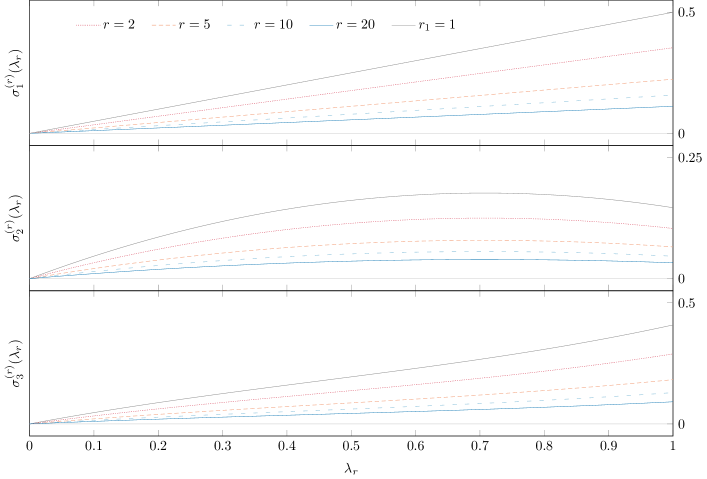
Refer to caption
Fig. 36: Evolution of the slope of the phase resonance solution (for large |x|𝑥|x|) with changing number of the mode n=r𝑛𝑟n=r.
(ϕ(r)(x))′′=1+λrcos(rϕ(r)).superscriptsuperscriptitalic-ϕ𝑟𝑥′′1subscript𝜆𝑟𝑟superscriptitalic-ϕ𝑟\displaystyle\left(\phi^{(r)}(x)\right)^{\prime\prime}\!=1+\lambda_{r}\cos\!\left(r\phi^{(r)}\right). (231)

The algorithm for solution is identical to the one presented above for the case with r=1𝑟1r=1, hence we only quote the results at each order. The zeroth-order correction is left unchanged, given by eq. (124). The first-order correction is:

ϕ(1)(r)(x)=±π[12λrr]\StrLen[\arglen]([xπ])+λrr[π\StrLenr[\arglen](r[xπ])(C\StrLenr[\arglen](r[xπ])12)sin[π2\StrLenr[\arglen](r[xπ])2]]+𝒪(λr2).superscriptsubscriptitalic-ϕ1𝑟𝑥plus-or-minus𝜋delimited-[]12subscript𝜆𝑟𝑟\StrLendelimited-[]\arglenabsentdelimited-[]𝑥𝜋subscript𝜆𝑟𝑟delimited-[]𝜋\StrLen𝑟delimited-[]\arglen𝑟delimited-[]𝑥𝜋minus-or-plus𝐶\StrLen𝑟delimited-[]\arglen𝑟delimited-[]𝑥𝜋12𝜋2\StrLen𝑟delimited-[]\arglensuperscript𝑟delimited-[]𝑥𝜋2𝒪superscriptsubscript𝜆𝑟2\displaystyle\phi_{(1)}^{(r)}(x)=\pm\,\pi\!\left[\vphantom{\Bigg{[}\Bigg{]}}\frac{1}{2}\,\frac{\lambda_{r}}{\sqrt{r}}\right]\!\!\StrLen{}[\arglen]\left(\vphantom{\left[\frac{x}{\sqrt{\pi}}\right]^{\!\!\!2\,}}\!\!\sqrt{\vphantom{|}}\!\left[\frac{x}{\sqrt{\pi}}\right]\!\right)\!+\frac{\lambda_{r}}{r}\!\left[\vphantom{\left[\Bigg{[}\Bigg{]}^{\!\!\!2\,}\right]^{\!\!\!2\,}}\pi\!\StrLen{r}[\arglen]\left(\vphantom{\left[\frac{x}{\sqrt{\pi}}\right]^{\!\!\!2\,}}\!\!\sqrt{\vphantom{|}r}\!\left[\frac{x}{\sqrt{\pi}}\right]\!\right)\!\!\left(\!\vphantom{\left[\left[\frac{x}{\sqrt{\pi}}r\right]^{\!\!\!2\,}\right]^{\!\!\!2\,}}C\!\StrLen{r}[\arglen]\left(\vphantom{\left[\frac{x}{\sqrt{\pi}}\right]^{\!\!\!2\,}}\!\!\sqrt{\vphantom{|}r}\!\left[\frac{x}{\sqrt{\pi}}\right]\!\right)\!\mp\frac{1}{2}\!\right)\!-\sin\!\left[\frac{\pi}{2}\!\StrLen{r}[\arglen]\left(\vphantom{\left[\frac{x}{\sqrt{\pi}}\right]^{\!\!\!2\,}}\!\!\sqrt{\vphantom{|}r}\!\left[\frac{x}{\sqrt{\pi}}\right]\!\right)^{\!\!\!2\,}\!\right]\!\right]\!+\mathcal{O}\!\left(\lambda_{r}^{2}\right). (232)

In the second-order correction we begin to notice the evolution of the terms from the original solution eq. (208):

ϕ(2)(r)(x)superscriptsubscriptitalic-ϕ2𝑟𝑥\displaystyle\phi_{(2)}^{(r)}(x) =±π[12λrr24λr2r]\StrLen[\arglen]([xπ])+π[18λr2r]absentplus-or-minus𝜋delimited-[]12subscript𝜆𝑟𝑟24superscriptsubscript𝜆𝑟2𝑟\StrLendelimited-[]\arglenabsentdelimited-[]𝑥𝜋𝜋delimited-[]18superscriptsubscript𝜆𝑟2𝑟\displaystyle=\pm\,\pi\!\left[\frac{1}{2}\,\frac{\lambda_{r}}{\sqrt{r}}-\frac{\sqrt{2}}{4}\,\frac{\lambda_{r}^{2}}{\sqrt{r}}\right]\!\!\StrLen{}[\arglen]\left(\vphantom{\left[\frac{x}{\sqrt{\pi}}\right]^{\!\!\!2\,}}\!\!\sqrt{\vphantom{|}}\!\left[\frac{x}{\sqrt{\pi}}\right]\!\right)\!+\pi\!\left[\vphantom{\Bigg{[}\Bigg{]}}\frac{1}{8}\,\frac{\lambda_{r}^{2}}{r}\right]
+λrr[π\StrLenr[\arglen](r[xπ±12λrr])(C\StrLenr[\arglen](r[xπ±12λrr])12)sin[π2\StrLenr[\arglen](r[xπ±12λrr])2]]subscript𝜆𝑟𝑟delimited-[]𝜋\StrLen𝑟delimited-[]\arglen𝑟delimited-[]plus-or-minus𝑥𝜋12subscript𝜆𝑟𝑟minus-or-plus𝐶\StrLen𝑟delimited-[]\arglen𝑟delimited-[]plus-or-minus𝑥𝜋12subscript𝜆𝑟𝑟12𝜋2\StrLen𝑟delimited-[]\arglensuperscript𝑟delimited-[]plus-or-minus𝑥𝜋12subscript𝜆𝑟𝑟2\displaystyle\quad+\frac{\lambda_{r}}{r}\!\left[\vphantom{\left[\Bigg{[}\Bigg{]}^{\!\!\!2\,}\right]^{\!\!\!2\,}}\pi\!\StrLen{r}[\arglen]\left(\vphantom{\left[\frac{x}{\sqrt{\pi}}\pm\frac{1}{2}\,\frac{\lambda_{r}}{\sqrt{r}}\right]^{\!\!\!2\,}}\!\!\sqrt{\vphantom{|}r}\!\left[\frac{x}{\sqrt{\pi}}\pm\frac{1}{2}\,\frac{\lambda_{r}}{\sqrt{r}}\right]\!\right)\!\!\left(\!\vphantom{\left[\left[\frac{x}{\sqrt{\pi}}r\pm\frac{1}{2}\,\frac{\lambda_{r}}{\sqrt{r}}\right]^{\!\!\!2\,}\right]^{\!\!\!2\,}}C\!\StrLen{r}[\arglen]\left(\vphantom{\left[\frac{x}{\sqrt{\pi}}\pm\frac{1}{2}\,\frac{\lambda_{r}}{\sqrt{r}}\right]^{\!\!\!2\,}}\!\!\sqrt{\vphantom{|}r}\!\left[\frac{x}{\sqrt{\pi}}\pm\frac{1}{2}\,\frac{\lambda_{r}}{\sqrt{r}}\right]\!\right)\!\mp\frac{1}{2}\!\right)\!-\sin\!\left[\frac{\pi}{2}\!\StrLen{r}[\arglen]\left(\vphantom{\left[\frac{x}{\sqrt{\pi}}\pm\frac{1}{2}\,\frac{\lambda_{r}}{\sqrt{r}}\right]^{\!\!\!2\,}}\!\!\sqrt{\vphantom{|}r}\!\left[\frac{x}{\sqrt{\pi}}\pm\frac{1}{2}\,\frac{\lambda_{r}}{\sqrt{r}}\right]\!\right)^{\!\!\!2\,}\!\right]\!\right] (233)
+λr2r[π2(C\StrLenr[\arglen](r[xπ])12)2π2\StrLen2r[\arglen](2r[xπ])(C\StrLen2r[\arglen](2r[xπ])12)+12sin[π2\StrLen2r[\arglen](2r[xπ])2]]+𝒪(λr3).superscriptsubscript𝜆𝑟2𝑟delimited-[]𝜋2superscriptminus-or-plus𝐶\StrLen𝑟delimited-[]\arglen𝑟delimited-[]𝑥𝜋122𝜋2\StrLen2𝑟delimited-[]\arglen2𝑟delimited-[]𝑥𝜋minus-or-plus𝐶\StrLen2𝑟delimited-[]\arglen2𝑟delimited-[]𝑥𝜋1212𝜋2\StrLen2𝑟delimited-[]\arglensuperscript2𝑟delimited-[]𝑥𝜋2𝒪superscriptsubscript𝜆𝑟3\displaystyle\quad+\frac{\lambda_{r}^{2}}{r}\!\left[\frac{\pi}{2}\!\left(\!\vphantom{\left[\left[\frac{x}{\sqrt{\pi}}r\right]^{\!\!\!2\,}\right]^{\!\!\!2\,}}C\!\StrLen{r}[\arglen]\left(\vphantom{\left[\frac{x}{\sqrt{\pi}}\right]^{\!\!\!2\,}}\!\!\sqrt{\vphantom{|}r}\!\left[\frac{x}{\sqrt{\pi}}\right]\!\right)\!\mp\frac{1}{2}\!\right)^{\!\!\!2\,}\!-\frac{\pi}{2}\!\StrLen{2r}[\arglen]\left(\vphantom{\left[\frac{x}{\sqrt{\pi}}\right]^{\!\!\!2\,}}\!\!\sqrt{\vphantom{|}2r}\!\left[\frac{x}{\sqrt{\pi}}\right]\!\right)\!\!\left(\!\vphantom{\left[\left[\frac{x}{\sqrt{\pi}}2r\right]^{\!\!\!2\,}\right]^{\!\!\!2\,}}C\!\StrLen{2r}[\arglen]\left(\vphantom{\left[\frac{x}{\sqrt{\pi}}\right]^{\!\!\!2\,}}\!\!\sqrt{\vphantom{|}2r}\!\left[\frac{x}{\sqrt{\pi}}\right]\!\right)\!\mp\frac{1}{2}\!\right)\!+\frac{1}{2}\,\sin\!\left[\frac{\pi}{2}\!\StrLen{2r}[\arglen]\left(\vphantom{\left[\frac{x}{\sqrt{\pi}}\right]^{\!\!\!2\,}}\!\!\sqrt{\vphantom{|}2r}\!\left[\frac{x}{\sqrt{\pi}}\right]\!\right)^{\!\!\!2\,}\!\right]\!\right]\!+\mathcal{O}\!\left(\lambda_{r}^{3}\right).

We can already notice some ways in which this result differs from the second-order correction with r=1𝑟1r=1, for instance the change of variables from x/π𝑥𝜋x/\!\sqrt{\pi} to rx/π𝑟𝑥𝜋\sqrt{r}\,x/\!\sqrt{\pi}, and the factor of 1/r1𝑟1/r added to the multipliers of the oscillating terms. Before we explain how this arises from the governing equation, we present the third-order result:

ϕ(3)(r)(x)=±π[12λrr24λr2r+33116λr3r]\StrLen[\arglen]([xπ])+π[18λr2r28λr3r]superscriptsubscriptitalic-ϕ3𝑟𝑥plus-or-minus𝜋delimited-[]12subscript𝜆𝑟𝑟24superscriptsubscript𝜆𝑟2𝑟33116superscriptsubscript𝜆𝑟3𝑟\StrLendelimited-[]\arglenabsentdelimited-[]𝑥𝜋𝜋delimited-[]18superscriptsubscript𝜆𝑟2𝑟28superscriptsubscript𝜆𝑟3𝑟\displaystyle\phi_{(3)}^{(r)}(x)=\pm\,\pi\!\left[\frac{1}{2}\,\frac{\lambda_{r}}{\sqrt{r}}-\frac{\sqrt{2}}{4}\,\frac{\lambda_{r}^{2}}{\sqrt{r}}+\frac{3\sqrt{3}-1}{16}\,\frac{\lambda_{r}^{3}}{\sqrt{r}}\right]\!\!\StrLen{}[\arglen]\left(\vphantom{\left[\frac{x}{\sqrt{\pi}}\right]^{\!\!\!2\,}}\!\!\sqrt{\vphantom{|}}\!\left[\frac{x}{\sqrt{\pi}}\right]\!\right)\!+\pi\!\left[\frac{1}{8}\,\frac{\lambda_{r}^{2}}{r}-\frac{\sqrt{2}}{8}\,\frac{\lambda_{r}^{3}}{r}\right]
+λrr[π\StrLenr[\arglen](r[xπ±σ2(r)(λr)])(C\StrLenr[\arglen](r[xπ±σ2(r)(λr)])12)sin[π2\StrLenr[\arglen](r[xπ±σ2(r)(λr)])2]]subscript𝜆𝑟𝑟delimited-[]𝜋\StrLen𝑟delimited-[]\arglen𝑟delimited-[]plus-or-minus𝑥𝜋superscriptsubscript𝜎2𝑟subscript𝜆𝑟minus-or-plus𝐶\StrLen𝑟delimited-[]\arglen𝑟delimited-[]plus-or-minus𝑥𝜋superscriptsubscript𝜎2𝑟subscript𝜆𝑟12𝜋2\StrLen𝑟delimited-[]\arglensuperscript𝑟delimited-[]plus-or-minus𝑥𝜋superscriptsubscript𝜎2𝑟subscript𝜆𝑟2\displaystyle\quad\quad\quad+\frac{\lambda_{r}}{r}\!\left[\vphantom{\left[\Bigg{[}\Bigg{]}^{\!\!\!2\,}\right]^{\!\!\!2\,}}\pi\!\StrLen{r}[\arglen]\left(\vphantom{\left[\frac{x}{\sqrt{\pi}}\pm\sigma_{2}^{(r)}(\lambda_{r})\right]^{\!\!\!2\,}}\!\!\sqrt{\vphantom{|}r}\!\left[\frac{x}{\sqrt{\pi}}\pm\sigma_{2}^{(r)}(\lambda_{r})\right]\!\right)\!\!\left(\!\vphantom{\left[\left[\frac{x}{\sqrt{\pi}}r\pm\sigma_{2}^{(r)}(\lambda_{r})\right]^{\!\!\!2\,}\right]^{\!\!\!2\,}}C\!\StrLen{r}[\arglen]\left(\vphantom{\left[\frac{x}{\sqrt{\pi}}\pm\sigma_{2}^{(r)}(\lambda_{r})\right]^{\!\!\!2\,}}\!\!\sqrt{\vphantom{|}r}\!\left[\frac{x}{\sqrt{\pi}}\pm\sigma_{2}^{(r)}(\lambda_{r})\right]\!\right)\!\mp\frac{1}{2}\!\right)\!-\sin\!\left[\frac{\pi}{2}\!\StrLen{r}[\arglen]\left(\vphantom{\left[\frac{x}{\sqrt{\pi}}\pm\sigma_{2}^{(r)}(\lambda_{r})\right]^{\!\!\!2\,}}\!\!\sqrt{\vphantom{|}r}\!\left[\frac{x}{\sqrt{\pi}}\pm\sigma_{2}^{(r)}(\lambda_{r})\right]\!\right)^{\!\!\!2\,}\!\right]\!\right]
+λr2r[π2(C\StrLenr[\arglen](r[xπ±12λrr])12)2+12sin[π2\StrLen2r[\arglen](2r[xπ±12λrr])2]\displaystyle\quad\quad\quad+\frac{\lambda_{r}^{2}}{r}\!\left[\frac{\pi}{2}\!\left(\!\vphantom{\left[\left[\frac{x}{\sqrt{\pi}}r\pm\frac{1}{2}\,\frac{\lambda_{r}}{\sqrt{r}}\right]^{\!\!\!2\,}\right]^{\!\!\!2\,}}C\!\StrLen{r}[\arglen]\left(\vphantom{\left[\frac{x}{\sqrt{\pi}}\pm\frac{1}{2}\,\frac{\lambda_{r}}{\sqrt{r}}\right]^{\!\!\!2\,}}\!\!\sqrt{\vphantom{|}r}\!\left[\frac{x}{\sqrt{\pi}}\pm\frac{1}{2}\,\frac{\lambda_{r}}{\sqrt{r}}\right]\!\right)\!\mp\frac{1}{2}\!\right)^{\!\!\!2\,}\!+\frac{1}{2}\,\sin\!\left[\frac{\pi}{2}\!\StrLen{2r}[\arglen]\left(\vphantom{\left[\frac{x}{\sqrt{\pi}}\pm\frac{1}{2}\,\frac{\lambda_{r}}{\sqrt{r}}\right]^{\!\!\!2\,}}\!\!\sqrt{\vphantom{|}2r}\!\left[\frac{x}{\sqrt{\pi}}\pm\frac{1}{2}\,\frac{\lambda_{r}}{\sqrt{r}}\right]\!\right)^{\!\!\!2\,}\!\right]\vphantom{\left[\Bigg{[}\Bigg{]}^{\!\!\!2\,}\right]^{\!\!\!2\,}}\right.
π2\StrLen2r[\arglen](2r[xπ±12λrr])(C\StrLen2r[\arglen](2r[xπ±12λrr])12)]\displaystyle\quad\quad\quad\quad\quad\quad\quad\quad\quad\quad\quad\quad\quad\quad\quad\quad\quad\quad\quad\quad\left.\vphantom{\left[\Bigg{[}\Bigg{]}^{\!\!\!2\,}\right]^{\!\!\!2\,}}-\frac{\pi}{2}\!\StrLen{2r}[\arglen]\left(\vphantom{\left[\frac{x}{\sqrt{\pi}}\pm\frac{1}{2}\,\frac{\lambda_{r}}{\sqrt{r}}\right]^{\!\!\!2\,}}\!\!\sqrt{\vphantom{|}2r}\!\left[\frac{x}{\sqrt{\pi}}\pm\frac{1}{2}\,\frac{\lambda_{r}}{\sqrt{r}}\right]\!\right)\!\!\left(\!\vphantom{\left[\left[\frac{x}{\sqrt{\pi}}2r\pm\frac{1}{2}\,\frac{\lambda_{r}}{\sqrt{r}}\right]^{\!\!\!2\,}\right]^{\!\!\!2\,}}C\!\StrLen{2r}[\arglen]\left(\vphantom{\left[\frac{x}{\sqrt{\pi}}\pm\frac{1}{2}\,\frac{\lambda_{r}}{\sqrt{r}}\right]^{\!\!\!2\,}}\!\!\sqrt{\vphantom{|}2r}\!\left[\frac{x}{\sqrt{\pi}}\pm\frac{1}{2}\,\frac{\lambda_{r}}{\sqrt{r}}\right]\!\right)\!\mp\frac{1}{2}\!\right)\!\right] (234)
+λr3r[π2cos[π2\StrLenr[\arglen](r[xπ])2](C\StrLenr[\arglen](r[xπ])12)2π2(C\StrLen2r[\arglen](2r[xπ])12)(C\StrLenr[\arglen](r[xπ])12)\displaystyle\quad\quad\quad+\frac{\lambda_{r}^{3}}{r}\!\left[\frac{\pi}{2}\,\cos\!\left[\frac{\pi}{2}\!\StrLen{r}[\arglen]\left(\vphantom{\left[\frac{x}{\sqrt{\pi}}\right]^{\!\!\!2\,}}\!\!\sqrt{\vphantom{|}r}\!\left[\frac{x}{\sqrt{\pi}}\right]\!\right)^{\!\!\!2\,}\!\right]\!\!\left(\!\vphantom{\left[\left[\frac{x}{\sqrt{\pi}}r\right]^{\!\!\!2\,}\right]^{\!\!\!2\,}}C\!\StrLen{r}[\arglen]\left(\vphantom{\left[\frac{x}{\sqrt{\pi}}\right]^{\!\!\!2\,}}\!\!\sqrt{\vphantom{|}r}\!\left[\frac{x}{\sqrt{\pi}}\right]\!\right)\!\mp\frac{1}{2}\!\right)^{\!\!\!2\,}\!\!-\frac{\pi}{\sqrt{2}}\!\left(\!\vphantom{\left[\left[\frac{x}{\sqrt{\pi}}2r\right]^{\!\!\!2\,}\right]^{\!\!\!2\,}}C\!\StrLen{2r}[\arglen]\left(\vphantom{\left[\frac{x}{\sqrt{\pi}}\right]^{\!\!\!2\,}}\!\!\sqrt{\vphantom{|}2r}\!\left[\frac{x}{\sqrt{\pi}}\right]\!\right)\!\mp\frac{1}{2}\!\right)\!\!\left(\!\vphantom{\left[\left[\frac{x}{\sqrt{\pi}}r\right]^{\!\!\!2\,}\right]^{\!\!\!2\,}}C\!\StrLen{r}[\arglen]\left(\vphantom{\left[\frac{x}{\sqrt{\pi}}\right]^{\!\!\!2\,}}\!\!\sqrt{\vphantom{|}r}\!\left[\frac{x}{\sqrt{\pi}}\right]\!\right)\!\mp\frac{1}{2}\!\right)\vphantom{\left[\left[\left[\Bigg{[}\Bigg{]}^{\!\!\!2\,}\right]^{\!\!\!2\,}\right]^{\!\!\!2\,}\right]^{\!\!\!2\,}}\right.
+3π8\StrLen3r[\arglen](3r[xπ])(C\StrLen3r[\arglen](3r[xπ])12)π8\StrLenr[\arglen](r[xπ])(C\StrLenr[\arglen](r[xπ])12)3𝜋8\StrLen3𝑟delimited-[]\arglen3𝑟delimited-[]𝑥𝜋minus-or-plus𝐶\StrLen3𝑟delimited-[]\arglen3𝑟delimited-[]𝑥𝜋12𝜋8\StrLen𝑟delimited-[]\arglen𝑟delimited-[]𝑥𝜋minus-or-plus𝐶\StrLen𝑟delimited-[]\arglen𝑟delimited-[]𝑥𝜋12\displaystyle\quad\quad\quad\quad\quad\quad\quad+\frac{3\pi}{8}\!\StrLen{3r}[\arglen]\left(\vphantom{\left[\frac{x}{\sqrt{\pi}}\right]^{\!\!\!2\,}}\!\!\sqrt{\vphantom{|}3r}\!\left[\frac{x}{\sqrt{\pi}}\right]\!\right)\!\!\left(\!\vphantom{\left[\left[\frac{x}{\sqrt{\pi}}3r\right]^{\!\!\!2\,}\right]^{\!\!\!2\,}}C\!\StrLen{3r}[\arglen]\left(\vphantom{\left[\frac{x}{\sqrt{\pi}}\right]^{\!\!\!2\,}}\!\!\sqrt{\vphantom{|}3r}\!\left[\frac{x}{\sqrt{\pi}}\right]\!\right)\!\mp\frac{1}{2}\!\right)\!-\frac{\pi}{8}\!\StrLen{r}[\arglen]\left(\vphantom{\left[\frac{x}{\sqrt{\pi}}\right]^{\!\!\!2\,}}\!\!\sqrt{\vphantom{|}r}\!\left[\frac{x}{\sqrt{\pi}}\right]\!\right)\!\!\left(\!\vphantom{\left[\left[\frac{x}{\sqrt{\pi}}r\right]^{\!\!\!2\,}\right]^{\!\!\!2\,}}C\!\StrLen{r}[\arglen]\left(\vphantom{\left[\frac{x}{\sqrt{\pi}}\right]^{\!\!\!2\,}}\!\!\sqrt{\vphantom{|}r}\!\left[\frac{x}{\sqrt{\pi}}\right]\!\right)\!\mp\frac{1}{2}\!\right)
38sin[π2\StrLen3r[\arglen](3r[xπ])2]+18sin[π2\StrLenr[\arglen](r[xπ])2]]+𝒪(λr4).\displaystyle\quad\quad\quad\quad\quad\quad\quad\quad\quad\quad\quad\left.\vphantom{\left[\left[\left[\Bigg{[}\Bigg{]}^{\!\!\!2\,}\right]^{\!\!\!2\,}\right]^{\!\!\!2\,}\right]^{\!\!\!2\,}}-\frac{3}{8}\,\sin\!\left[\frac{\pi}{2}\!\StrLen{3r}[\arglen]\left(\vphantom{\left[\frac{x}{\sqrt{\pi}}\right]^{\!\!\!2\,}}\!\!\sqrt{\vphantom{|}3r}\!\left[\frac{x}{\sqrt{\pi}}\right]\!\right)^{\!\!\!2\,}\!\right]\!+\frac{1}{8}\,\sin\!\left[\frac{\pi}{2}\!\StrLen{r}[\arglen]\left(\vphantom{\left[\frac{x}{\sqrt{\pi}}\right]^{\!\!\!2\,}}\!\!\sqrt{\vphantom{|}r}\!\left[\frac{x}{\sqrt{\pi}}\right]\!\right)^{\!\!\!2\,}\!\right]\!\right]\!+\mathcal{O}\!\left(\lambda_{r}^{4}\right).

These results can be obtained from the ones involving λ1λsubscript𝜆1𝜆\lambda_{1}\equiv\lambda by transforming eq. (122) with a change of variables:

which yields eq. (231), hence the solutions to this equation can be found from eq. (122) by applying a change of variables. It is interesting to see how the number of the mode r𝑟r affects the graphical behaviour of the solution. In Figure 19 we have plotted the effect of the mode number r𝑟r on the correction ϕ3(r)(x)superscriptsubscriptitalic-ϕ3𝑟𝑥{\phi_{3}}^{(r)}(x), and in Figure 36 we see the effect of r𝑟r on the slope of the solution. The validity of solutions (232) – (234) is confirmed graphically in Figure 37.
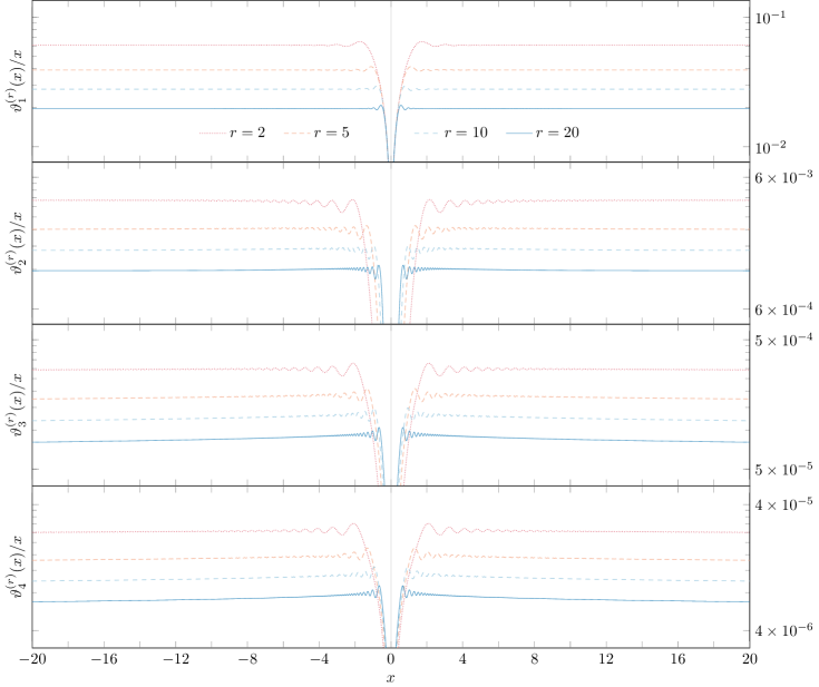
Refer to caption
Fig. 37: Graphical validation of the phase resonance equation with a single n1𝑛1n\neq 1 mode. solutions (232) – (234)

IV Phase resonance equation with two distinct modes

As an interlude to solving the multi-mode version of the phase resonance equation, we present the solution for two modes on the right-hand side, labelled by integers r𝑟r and s𝑠s. Without loss of generality, we can let let r<s𝑟𝑠r<s.

(ϕ(r,s)(x))′′=1+λrcos(rϕ)+λscos(sϕ).superscriptsuperscriptitalic-ϕ𝑟𝑠𝑥′′1subscript𝜆𝑟𝑟italic-ϕsubscript𝜆𝑠𝑠italic-ϕ\displaystyle\left(\phi^{(r,s)}(x)\right)^{\prime\prime}=1+\lambda_{r}\cos\left(r\phi\right)+\lambda_{s}\cos\left(s\phi\right). (142)

The zeroth-order solution remains unchanged, ϕ0(r,s)=x2/2superscriptsubscriptitalic-ϕ0𝑟𝑠superscript𝑥22\phi_{0}^{(r,s)}=x^{2}/2. The first-order correction can be written in the form:

ϕ(1)(r,s)(x)=l{r,s}{±π2λll\StrLen[\arglen]([xπ])+λll[π\StrLenl[\arglen](l[xπ])(C\StrLenl[\arglen](l[xπ])12)sin[π2\StrLenl[\arglen](l[xπ])2]]},superscriptsubscriptitalic-ϕ1𝑟𝑠𝑥subscript𝑙𝑟𝑠plus-or-minus𝜋2subscript𝜆𝑙𝑙\StrLendelimited-[]\arglenabsentdelimited-[]𝑥𝜋subscript𝜆𝑙𝑙delimited-[]𝜋\StrLen𝑙delimited-[]\arglen𝑙delimited-[]𝑥𝜋minus-or-plus𝐶\StrLen𝑙delimited-[]\arglen𝑙delimited-[]𝑥𝜋12𝜋2\StrLen𝑙delimited-[]\arglensuperscript𝑙delimited-[]𝑥𝜋2\displaystyle\phi_{(1)}^{(r,s)}(x)=\sum_{l\in\{r,s\}}\!\left\{\vphantom{\left[\left[\left[\Bigg{[}\Bigg{]}^{\!\!\!2\,}\right]^{\!\!\!2\,}\right]^{\!\!\!2\,}\right]^{\!\!\!2\,}}\!\!\pm\frac{\pi}{2}\frac{\lambda_{l}}{\sqrt{l}}\!\StrLen{}[\arglen]\left(\vphantom{\left[\frac{x}{\sqrt{\pi}}\right]^{\!\!\!2\,}}\!\!\sqrt{\vphantom{|}}\!\left[\frac{x}{\sqrt{\pi}}\right]\!\right)\!+\frac{\lambda_{l}}{l}\!\left[\vphantom{\left[\Bigg{[}\Bigg{]}^{\!\!\!2\,}\right]^{\!\!\!2\,}}\pi\!\StrLen{l}[\arglen]\left(\vphantom{\left[\frac{x}{\sqrt{\pi}}\right]^{\!\!\!2\,}}\!\!\sqrt{\vphantom{|}l}\!\left[\frac{x}{\sqrt{\pi}}\right]\!\right)\!\!\left(\!\vphantom{\left[\left[\frac{x}{\sqrt{\pi}}l\right]^{\!\!\!2\,}\right]^{\!\!\!2\,}}C\!\StrLen{l}[\arglen]\left(\vphantom{\left[\frac{x}{\sqrt{\pi}}\right]^{\!\!\!2\,}}\!\!\sqrt{\vphantom{|}l}\!\left[\frac{x}{\sqrt{\pi}}\right]\!\right)\!\mp\frac{1}{2}\!\right)\!-\sin\!\left[\frac{\pi}{2}\!\StrLen{l}[\arglen]\left(\vphantom{\left[\frac{x}{\sqrt{\pi}}\right]^{\!\!\!2\,}}\!\!\sqrt{\vphantom{|}l}\!\left[\frac{x}{\sqrt{\pi}}\right]\!\right)^{\!\!\!2\,}\!\right]\!\right]\!\!\right\}, (236)

i.e., the two separate solutions do not mix at first order, and effectively ϕ(1)(r,s)(x)=ϕ(1)(r)(x)+ϕ(1)(s)(x)superscriptsubscriptitalic-ϕ1𝑟𝑠𝑥superscriptsubscriptitalic-ϕ1𝑟𝑥superscriptsubscriptitalic-ϕ1𝑠𝑥\phi_{(1)}^{(r,s)}(x)=\phi_{(1)}^{(r)}(x)+\phi_{(1)}^{(s)}(x).

At next order, however, mixing occurs, since we need to substitute the above expression (236) in both terms on the right-hand side of eq. (142). The second-order correction to the original solution can be found to be a combination of (modified) single-mode corrections plus a new mixing term at second order.

ϕ(2)(r,s)(x)=±π[12(λrr+λss)24(λr2r+λs2s)+14((sr)3/2(r+s)3/2)λrrλss]\StrLen[\arglen]([xπ])+π8(λrr+λss)2superscriptsubscriptitalic-ϕ2𝑟𝑠𝑥plus-or-minus𝜋delimited-[]12subscript𝜆𝑟𝑟subscript𝜆𝑠𝑠24superscriptsubscript𝜆𝑟2𝑟superscriptsubscript𝜆𝑠2𝑠14superscript𝑠𝑟32superscript𝑟𝑠32subscript𝜆𝑟𝑟subscript𝜆𝑠𝑠\StrLendelimited-[]\arglenabsentdelimited-[]𝑥𝜋𝜋8superscriptsubscript𝜆𝑟𝑟subscript𝜆𝑠𝑠2\displaystyle\phi_{(2)}^{(r,s)}(x)=\pm\,\pi\!\left[\vphantom{\Bigg{[}\Bigg{]}^{\!\!\!2\,}}\frac{1}{2}\!\left(\!\frac{\lambda_{r}}{\sqrt{r}}+\frac{\lambda_{s}}{\sqrt{s}}\!\right)\!-\frac{\sqrt{2}}{4}\!\left(\vphantom{\Bigg{[}\Bigg{]}}\!\frac{\lambda_{r}^{2}}{\sqrt{r}}+\frac{\lambda_{s}^{2}}{\sqrt{s}}\!\right)+\frac{1}{4}\!\left(\left(s-r\right)^{\nicefrac{{3}}{{2}}}-\left(r+s\right)^{\nicefrac{{3}}{{2}}}\right)\!\frac{\lambda_{r}}{r}\frac{\lambda_{s}}{s}\right]\!\!\StrLen{}[\arglen]\left(\vphantom{\left[\frac{x}{\sqrt{\pi}}\right]^{\!\!\!2\,}}\!\!\sqrt{\vphantom{|}}\!\left[\frac{x}{\sqrt{\pi}}\right]\!\right)+\frac{\pi}{8}\!\left(\!\frac{\lambda_{r}}{\sqrt{r}}+\frac{\lambda_{s}}{\sqrt{s}}\!\right)^{\!\!\!2\,}
+λrr[π\StrLenr[\arglen](r[xπ±12(λrr+λss)])(C\StrLenr[\arglen](r[xπ±12(λrr+λss)])12)sin[π2\StrLenr[\arglen](r[xπ±12(λrr+λss)])2]]subscript𝜆𝑟𝑟delimited-[]𝜋\StrLen𝑟delimited-[]\arglen𝑟delimited-[]plus-or-minus𝑥𝜋12subscript𝜆𝑟𝑟subscript𝜆𝑠𝑠minus-or-plus𝐶\StrLen𝑟delimited-[]\arglen𝑟delimited-[]plus-or-minus𝑥𝜋12subscript𝜆𝑟𝑟subscript𝜆𝑠𝑠12𝜋2\StrLen𝑟delimited-[]\arglensuperscript𝑟delimited-[]plus-or-minus𝑥𝜋12subscript𝜆𝑟𝑟subscript𝜆𝑠𝑠2\displaystyle+\frac{\lambda_{r}}{r}\!\left[\vphantom{\left[\left[\left[\Bigg{[}\Bigg{]}^{\!\!\!2\,}\right]^{\!\!\!2\,}\right]^{\!\!\!2\,}\right]^{\!\!\!2\,}}\pi\!\StrLen{r}[\arglen]\left(\vphantom{\left[\frac{x}{\sqrt{\pi}}\pm\frac{1}{2}\!\left(\!\frac{\lambda_{r}}{\sqrt{r}}+\frac{\lambda_{s}}{\sqrt{s}}\!\right)\vphantom{\left[\frac{\lambda_{r}}{\sqrt{r}}\right]^{\!\!\!2\,}}\!\!\right]^{\!\!\!2\,}}\!\!\sqrt{\vphantom{|}r}\!\left[\frac{x}{\sqrt{\pi}}\pm\frac{1}{2}\!\left(\!\frac{\lambda_{r}}{\sqrt{r}}+\frac{\lambda_{s}}{\sqrt{s}}\!\right)\vphantom{\left[\frac{\lambda_{r}}{\sqrt{r}}\right]^{\!\!\!2\,}}\!\!\right]\!\right)\!\!\left(\!\vphantom{\left[\left[\frac{x}{\sqrt{\pi}}r\pm\frac{1}{2}\!\left(\!\frac{\lambda_{r}}{\sqrt{r}}+\frac{\lambda_{s}}{\sqrt{s}}\!\right)\vphantom{\left[\frac{\lambda_{r}}{\sqrt{r}}\right]^{\!\!\!2\,}}\!\!\right]^{\!\!\!2\,}\right]^{\!\!\!2\,}}C\!\StrLen{r}[\arglen]\left(\vphantom{\left[\frac{x}{\sqrt{\pi}}\pm\frac{1}{2}\!\left(\!\frac{\lambda_{r}}{\sqrt{r}}+\frac{\lambda_{s}}{\sqrt{s}}\!\right)\vphantom{\left[\frac{\lambda_{r}}{\sqrt{r}}\right]^{\!\!\!2\,}}\!\!\right]^{\!\!\!2\,}}\!\!\sqrt{\vphantom{|}r}\!\left[\frac{x}{\sqrt{\pi}}\pm\frac{1}{2}\!\left(\!\frac{\lambda_{r}}{\sqrt{r}}+\frac{\lambda_{s}}{\sqrt{s}}\!\right)\vphantom{\left[\frac{\lambda_{r}}{\sqrt{r}}\right]^{\!\!\!2\,}}\!\!\right]\!\right)\!\mp\frac{1}{2}\!\right)\!-\sin\!\left[\frac{\pi}{2}\!\StrLen{r}[\arglen]\left(\vphantom{\left[\frac{x}{\sqrt{\pi}}\pm\frac{1}{2}\!\left(\!\frac{\lambda_{r}}{\sqrt{r}}+\frac{\lambda_{s}}{\sqrt{s}}\!\right)\vphantom{\left[\frac{\lambda_{r}}{\sqrt{r}}\right]^{\!\!\!2\,}}\!\!\right]^{\!\!\!2\,}}\!\!\sqrt{\vphantom{|}r}\!\left[\frac{x}{\sqrt{\pi}}\pm\frac{1}{2}\!\left(\!\frac{\lambda_{r}}{\sqrt{r}}+\frac{\lambda_{s}}{\sqrt{s}}\!\right)\vphantom{\left[\frac{\lambda_{r}}{\sqrt{r}}\right]^{\!\!\!2\,}}\!\!\right]\!\right)^{\!\!\!2\,}\!\right]\!\right]
+λss[π\StrLens[\arglen](s[xπ±12(λrr+λss)])(C\StrLens[\arglen](s[xπ±12(λrr+λss)])12)sin[π2\StrLens[\arglen](s[xπ±12(λrr+λss)])2]]subscript𝜆𝑠𝑠delimited-[]𝜋\StrLen𝑠delimited-[]\arglen𝑠delimited-[]plus-or-minus𝑥𝜋12subscript𝜆𝑟𝑟subscript𝜆𝑠𝑠minus-or-plus𝐶\StrLen𝑠delimited-[]\arglen𝑠delimited-[]plus-or-minus𝑥𝜋12subscript𝜆𝑟𝑟subscript𝜆𝑠𝑠12𝜋2\StrLen𝑠delimited-[]\arglensuperscript𝑠delimited-[]plus-or-minus𝑥𝜋12subscript𝜆𝑟𝑟subscript𝜆𝑠𝑠2\displaystyle+\frac{\lambda_{s}}{s}\!\left[\vphantom{\left[\left[\left[\Bigg{[}\Bigg{]}^{\!\!\!2\,}\right]^{\!\!\!2\,}\right]^{\!\!\!2\,}\right]^{\!\!\!2\,}}\pi\!\StrLen{s}[\arglen]\left(\vphantom{\left[\frac{x}{\sqrt{\pi}}\pm\frac{1}{2}\!\left(\!\frac{\lambda_{r}}{\sqrt{r}}+\frac{\lambda_{s}}{\sqrt{s}}\!\right)\vphantom{\left[\frac{\lambda_{r}}{\sqrt{r}}\right]^{\!\!\!2\,}}\!\!\right]^{\!\!\!2\,}}\!\!\sqrt{\vphantom{|}s}\!\left[\frac{x}{\sqrt{\pi}}\pm\frac{1}{2}\!\left(\!\frac{\lambda_{r}}{\sqrt{r}}+\frac{\lambda_{s}}{\sqrt{s}}\!\right)\vphantom{\left[\frac{\lambda_{r}}{\sqrt{r}}\right]^{\!\!\!2\,}}\!\!\right]\!\right)\!\!\left(\!\vphantom{\left[\left[\frac{x}{\sqrt{\pi}}s\pm\frac{1}{2}\!\left(\!\frac{\lambda_{r}}{\sqrt{r}}+\frac{\lambda_{s}}{\sqrt{s}}\!\right)\vphantom{\left[\frac{\lambda_{r}}{\sqrt{r}}\right]^{\!\!\!2\,}}\!\!\right]^{\!\!\!2\,}\right]^{\!\!\!2\,}}C\!\StrLen{s}[\arglen]\left(\vphantom{\left[\frac{x}{\sqrt{\pi}}\pm\frac{1}{2}\!\left(\!\frac{\lambda_{r}}{\sqrt{r}}+\frac{\lambda_{s}}{\sqrt{s}}\!\right)\vphantom{\left[\frac{\lambda_{r}}{\sqrt{r}}\right]^{\!\!\!2\,}}\!\!\right]^{\!\!\!2\,}}\!\!\sqrt{\vphantom{|}s}\!\left[\frac{x}{\sqrt{\pi}}\pm\frac{1}{2}\!\left(\!\frac{\lambda_{r}}{\sqrt{r}}+\frac{\lambda_{s}}{\sqrt{s}}\!\right)\vphantom{\left[\frac{\lambda_{r}}{\sqrt{r}}\right]^{\!\!\!2\,}}\!\!\right]\!\right)\!\mp\frac{1}{2}\!\right)\!-\sin\!\left[\frac{\pi}{2}\!\StrLen{s}[\arglen]\left(\vphantom{\left[\frac{x}{\sqrt{\pi}}\pm\frac{1}{2}\!\left(\!\frac{\lambda_{r}}{\sqrt{r}}+\frac{\lambda_{s}}{\sqrt{s}}\!\right)\vphantom{\left[\frac{\lambda_{r}}{\sqrt{r}}\right]^{\!\!\!2\,}}\!\!\right]^{\!\!\!2\,}}\!\!\sqrt{\vphantom{|}s}\!\left[\frac{x}{\sqrt{\pi}}\pm\frac{1}{2}\!\left(\!\frac{\lambda_{r}}{\sqrt{r}}+\frac{\lambda_{s}}{\sqrt{s}}\!\right)\vphantom{\left[\frac{\lambda_{r}}{\sqrt{r}}\right]^{\!\!\!2\,}}\!\!\right]\!\right)^{\!\!\!2\,}\!\right]\!\right]
+π2(λrr(C\StrLenr[\arglen](r[xπ])12)+λss(C\StrLens[\arglen](s[xπ])12))2𝜋2superscriptsubscript𝜆𝑟𝑟minus-or-plus𝐶\StrLen𝑟delimited-[]\arglen𝑟delimited-[]𝑥𝜋12subscript𝜆𝑠𝑠minus-or-plus𝐶\StrLen𝑠delimited-[]\arglen𝑠delimited-[]𝑥𝜋122\displaystyle+\frac{\pi}{2}\!\left(\vphantom{\left[\Bigg{[}\Bigg{]}^{\!\!\!2\,}\right]^{\!\!\!2\,}}\!\frac{\lambda_{r}}{\sqrt{r}}\!\left(\!\vphantom{\left[\left[\frac{x}{\sqrt{\pi}}r\right]^{\!\!\!2\,}\right]^{\!\!\!2\,}}C\!\StrLen{r}[\arglen]\left(\vphantom{\left[\frac{x}{\sqrt{\pi}}\right]^{\!\!\!2\,}}\!\!\sqrt{\vphantom{|}r}\!\left[\frac{x}{\sqrt{\pi}}\right]\!\right)\!\mp\frac{1}{2}\!\right)\!+\frac{\lambda_{s}}{\sqrt{s}}\!\left(\!\vphantom{\left[\left[\frac{x}{\sqrt{\pi}}s\right]^{\!\!\!2\,}\right]^{\!\!\!2\,}}C\!\StrLen{s}[\arglen]\left(\vphantom{\left[\frac{x}{\sqrt{\pi}}\right]^{\!\!\!2\,}}\!\!\sqrt{\vphantom{|}s}\!\left[\frac{x}{\sqrt{\pi}}\right]\!\right)\!\mp\frac{1}{2}\!\right)\!\!\right)^{\!\!\!2\,}
+π2λrrλss((sr)\StrLensr[\arglen](sr[xπ])(C\StrLensr[\arglen](sr[xπ])12)(r+s)\StrLenr+s[\arglen](r+s[xπ])(C\StrLenr+s[\arglen](r+s[xπ])12))𝜋2subscript𝜆𝑟𝑟subscript𝜆𝑠𝑠𝑠𝑟\StrLen𝑠𝑟delimited-[]\arglen𝑠𝑟delimited-[]𝑥𝜋minus-or-plus𝐶\StrLen𝑠𝑟delimited-[]\arglen𝑠𝑟delimited-[]𝑥𝜋12𝑟𝑠\StrLen𝑟𝑠delimited-[]\arglen𝑟𝑠delimited-[]𝑥𝜋minus-or-plus𝐶\StrLen𝑟𝑠delimited-[]\arglen𝑟𝑠delimited-[]𝑥𝜋12\displaystyle\quad\quad+\frac{\pi}{2}\,\frac{\lambda_{r}}{r}\frac{\lambda_{s}}{s}\!\left(\vphantom{\left[\Bigg{[}\Bigg{]}^{\!\!\!2\,}\right]^{\!\!\!2\,}}\!\!\left(s-r\right)\!\StrLen{s-r}[\arglen]\left(\vphantom{\left[\frac{x}{\sqrt{\pi}}\right]^{\!\!\!2\,}}\!\!\sqrt{\vphantom{|}s-r}\!\left[\frac{x}{\sqrt{\pi}}\right]\!\right)\!\!\left(\!\vphantom{\left[\left[\frac{x}{\sqrt{\pi}}s-r\right]^{\!\!\!2\,}\right]^{\!\!\!2\,}}C\!\StrLen{s-r}[\arglen]\left(\vphantom{\left[\frac{x}{\sqrt{\pi}}\right]^{\!\!\!2\,}}\!\!\sqrt{\vphantom{|}s-r}\!\left[\frac{x}{\sqrt{\pi}}\right]\!\right)\!\mp\frac{1}{2}\!\right)\!-\left(r+s\right)\!\StrLen{r+s}[\arglen]\left(\vphantom{\left[\frac{x}{\sqrt{\pi}}\right]^{\!\!\!2\,}}\!\!\sqrt{\vphantom{|}r+s}\!\left[\frac{x}{\sqrt{\pi}}\right]\!\right)\!\!\left(\!\vphantom{\left[\left[\frac{x}{\sqrt{\pi}}r+s\right]^{\!\!\!2\,}\right]^{\!\!\!2\,}}C\!\StrLen{r+s}[\arglen]\left(\vphantom{\left[\frac{x}{\sqrt{\pi}}\right]^{\!\!\!2\,}}\!\!\sqrt{\vphantom{|}r+s}\!\left[\frac{x}{\sqrt{\pi}}\right]\!\right)\!\mp\frac{1}{2}\!\right)\!\!\right)
π2(λr2r\StrLen2r[\arglen](2r[xπ])(C\StrLen2r[\arglen](2r[xπ])12)+λs2s\StrLen2s[\arglen](2s[xπ])(C\StrLen2s[\arglen](2s[xπ])12))𝜋2superscriptsubscript𝜆𝑟2𝑟\StrLen2𝑟delimited-[]\arglen2𝑟delimited-[]𝑥𝜋minus-or-plus𝐶\StrLen2𝑟delimited-[]\arglen2𝑟delimited-[]𝑥𝜋12superscriptsubscript𝜆𝑠2𝑠\StrLen2𝑠delimited-[]\arglen2𝑠delimited-[]𝑥𝜋minus-or-plus𝐶\StrLen2𝑠delimited-[]\arglen2𝑠delimited-[]𝑥𝜋12\displaystyle\quad\quad\quad\quad\quad\quad-\frac{\pi}{2}\!\left(\vphantom{\left[\Bigg{[}\Bigg{]}^{\!\!\!2\,}\right]^{\!\!\!2\,}}\!\frac{\lambda_{r}^{2}}{r}\!\StrLen{2r}[\arglen]\left(\vphantom{\left[\frac{x}{\sqrt{\pi}}\right]^{\!\!\!2\,}}\!\!\sqrt{\vphantom{|}2r}\!\left[\frac{x}{\sqrt{\pi}}\right]\!\right)\!\!\left(\!\vphantom{\left[\left[\frac{x}{\sqrt{\pi}}2r\right]^{\!\!\!2\,}\right]^{\!\!\!2\,}}C\!\StrLen{2r}[\arglen]\left(\vphantom{\left[\frac{x}{\sqrt{\pi}}\right]^{\!\!\!2\,}}\!\!\sqrt{\vphantom{|}2r}\!\left[\frac{x}{\sqrt{\pi}}\right]\!\right)\!\mp\frac{1}{2}\!\right)\!+\frac{\lambda_{s}^{2}}{s}\!\StrLen{2s}[\arglen]\left(\vphantom{\left[\frac{x}{\sqrt{\pi}}\right]^{\!\!\!2\,}}\!\!\sqrt{\vphantom{|}2s}\!\left[\frac{x}{\sqrt{\pi}}\right]\!\right)\!\!\left(\!\vphantom{\left[\left[\frac{x}{\sqrt{\pi}}2s\right]^{\!\!\!2\,}\right]^{\!\!\!2\,}}C\!\StrLen{2s}[\arglen]\left(\vphantom{\left[\frac{x}{\sqrt{\pi}}\right]^{\!\!\!2\,}}\!\!\sqrt{\vphantom{|}2s}\!\left[\frac{x}{\sqrt{\pi}}\right]\!\right)\!\mp\frac{1}{2}\!\right)\!\!\right)
12λrrλss((sr)sin[π2\StrLensr[\arglen](sr[xπ])2](r+s)sin[π2\StrLenr+s[\arglen](r+s[xπ])2])12subscript𝜆𝑟𝑟subscript𝜆𝑠𝑠𝑠𝑟𝜋2\StrLen𝑠𝑟delimited-[]\arglensuperscript𝑠𝑟delimited-[]𝑥𝜋2𝑟𝑠𝜋2\StrLen𝑟𝑠delimited-[]\arglensuperscript𝑟𝑠delimited-[]𝑥𝜋2\displaystyle\quad\quad\quad\quad\quad\quad\quad\quad\quad\quad-\frac{1}{2}\,\frac{\lambda_{r}}{r}\frac{\lambda_{s}}{s}\!\left(\vphantom{\left[\Bigg{[}\Bigg{]}^{\!\!\!2\,}\right]^{\!\!\!2\,}}\!\left(s-r\right)\,\sin\!\left[\frac{\pi}{2}\!\StrLen{s-r}[\arglen]\left(\vphantom{\left[\frac{x}{\sqrt{\pi}}\right]^{\!\!\!2\,}}\!\!\sqrt{\vphantom{|}s-r}\!\left[\frac{x}{\sqrt{\pi}}\right]\!\right)^{\!\!\!2\,}\!\right]\!-\left(r+s\right)\,\sin\!\left[\frac{\pi}{2}\!\StrLen{r+s}[\arglen]\left(\vphantom{\left[\frac{x}{\sqrt{\pi}}\right]^{\!\!\!2\,}}\!\!\sqrt{\vphantom{|}r+s}\!\left[\frac{x}{\sqrt{\pi}}\right]\!\right)^{\!\!\!2\,}\!\right]\!\right)
+12(λr2rsin[π2\StrLen2r[\arglen](2r[xπ])2]+λs2ssin[π2\StrLen2s[\arglen](2s[xπ])2])=12superscriptsubscript𝜆𝑟2𝑟𝜋2\StrLen2𝑟delimited-[]\arglensuperscript2𝑟delimited-[]𝑥𝜋2superscriptsubscript𝜆𝑠2𝑠𝜋2\StrLen2𝑠delimited-[]\arglensuperscript2𝑠delimited-[]𝑥𝜋2absent\displaystyle\quad\quad\quad\quad\quad\quad\quad\quad\quad\quad\quad\quad\quad\quad+\frac{1}{2}\!\left(\vphantom{\left[\Bigg{[}\Bigg{]}^{\!\!\!2\,}\right]^{\!\!\!2\,}}\!\frac{\lambda_{r}^{2}}{r}\,\sin\!\left[\frac{\pi}{2}\!\StrLen{2r}[\arglen]\left(\vphantom{\left[\frac{x}{\sqrt{\pi}}\right]^{\!\!\!2\,}}\!\!\sqrt{\vphantom{|}2r}\!\left[\frac{x}{\sqrt{\pi}}\right]\!\right)^{\!\!\!2\,}\!\right]\!+\frac{\lambda_{s}^{2}}{s}\,\sin\!\left[\frac{\pi}{2}\!\StrLen{2s}[\arglen]\left(\vphantom{\left[\frac{x}{\sqrt{\pi}}\right]^{\!\!\!2\,}}\!\!\sqrt{\vphantom{|}2s}\!\left[\frac{x}{\sqrt{\pi}}\right]\!\right)^{\!\!\!2\,}\!\right]\!\right)= (237)
=l{r,s}{±π[12λll24λl2l]\StrLenl[\arglen](l[xπ])+π[18λl2l]\displaystyle=\!\sum_{l\in\{r,s\}}\!\left\{\vphantom{\left[\left[\left[\Bigg{[}\Bigg{]}^{\!\!\!2\,}\right]^{\!\!\!2\,}\right]^{\!\!\!2\,}\right]^{\!\!\!2\,}}\!\pm\,\pi\!\left[\frac{1}{2}\,\frac{\lambda_{l}}{l}-\frac{\sqrt{2}}{4}\,\frac{\lambda_{l}^{2}}{l}\right]\!\!\StrLen{l}[\arglen]\left(\vphantom{\left[\frac{x}{\sqrt{\pi}}\right]^{\!\!\!2\,}}\!\!\sqrt{\vphantom{|}l}\!\left[\frac{x}{\sqrt{\pi}}\right]\!\right)\!+\pi\!\left[\vphantom{\Bigg{[}\Bigg{]}}\frac{1}{8}\,\frac{\lambda_{l}^{2}}{l}\right]\right.
+λll[π\StrLenl[\arglen](l[xπ±12(λll+λl¯l¯)])(C\StrLenl[\arglen](l[xπ±12(λll+λl¯l¯)])12)sin[π2\StrLenl[\arglen](l[xπ±12(λll+λl¯l¯)])2]]subscript𝜆𝑙𝑙delimited-[]𝜋\StrLen𝑙delimited-[]\arglen𝑙delimited-[]plus-or-minus𝑥𝜋12subscript𝜆𝑙𝑙subscript𝜆¯𝑙¯𝑙minus-or-plus𝐶\StrLen𝑙delimited-[]\arglen𝑙delimited-[]plus-or-minus𝑥𝜋12subscript𝜆𝑙𝑙subscript𝜆¯𝑙¯𝑙12𝜋2\StrLen𝑙delimited-[]\arglensuperscript𝑙delimited-[]plus-or-minus𝑥𝜋12subscript𝜆𝑙𝑙subscript𝜆¯𝑙¯𝑙2\displaystyle\quad+\frac{\lambda_{l}}{l}\!\left[\vphantom{\left[\left[\left[\Bigg{[}\Bigg{]}^{\!\!\!2\,}\right]^{\!\!\!2\,}\right]^{\!\!\!2\,}\right]^{\!\!\!2\,}}\pi\!\StrLen{l}[\arglen]\left(\vphantom{\left[\frac{x}{\sqrt{\pi}}\pm\frac{1}{2}\!\left(\!\frac{\lambda_{l}}{\sqrt{l}}+\frac{\lambda_{\bar{l}}}{\sqrt{\bar{l}\phantom{\,}}}\!\right)\vphantom{\left[\frac{\lambda_{r}}{\sqrt{r}}\right]^{\!\!\!2\,}}\!\!\right]^{\!\!\!2\,}}\!\!\sqrt{\vphantom{|}l}\!\left[\frac{x}{\sqrt{\pi}}\pm\frac{1}{2}\!\left(\!\frac{\lambda_{l}}{\sqrt{l}}+\frac{\lambda_{\bar{l}}}{\sqrt{\bar{l}\phantom{\,}}}\!\right)\vphantom{\left[\frac{\lambda_{r}}{\sqrt{r}}\right]^{\!\!\!2\,}}\!\!\right]\!\right)\!\!\left(\!\vphantom{\left[\left[\frac{x}{\sqrt{\pi}}l\pm\frac{1}{2}\!\left(\!\frac{\lambda_{l}}{\sqrt{l}}+\frac{\lambda_{\bar{l}}}{\sqrt{\bar{l}\phantom{\,}}}\!\right)\vphantom{\left[\frac{\lambda_{r}}{\sqrt{r}}\right]^{\!\!\!2\,}}\!\!\right]^{\!\!\!2\,}\right]^{\!\!\!2\,}}C\!\StrLen{l}[\arglen]\left(\vphantom{\left[\frac{x}{\sqrt{\pi}}\pm\frac{1}{2}\!\left(\!\frac{\lambda_{l}}{\sqrt{l}}+\frac{\lambda_{\bar{l}}}{\sqrt{\bar{l}\phantom{\,}}}\!\right)\vphantom{\left[\frac{\lambda_{r}}{\sqrt{r}}\right]^{\!\!\!2\,}}\!\!\right]^{\!\!\!2\,}}\!\!\sqrt{\vphantom{|}l}\!\left[\frac{x}{\sqrt{\pi}}\pm\frac{1}{2}\!\left(\!\frac{\lambda_{l}}{\sqrt{l}}+\frac{\lambda_{\bar{l}}}{\sqrt{\bar{l}\phantom{\,}}}\!\right)\vphantom{\left[\frac{\lambda_{r}}{\sqrt{r}}\right]^{\!\!\!2\,}}\!\!\right]\!\right)\!\mp\frac{1}{2}\!\right)\!-\sin\!\left[\frac{\pi}{2}\!\StrLen{l}[\arglen]\left(\vphantom{\left[\frac{x}{\sqrt{\pi}}\pm\frac{1}{2}\!\left(\!\frac{\lambda_{l}}{\sqrt{l}}+\frac{\lambda_{\bar{l}}}{\sqrt{\bar{l}\phantom{\,}}}\!\right)\vphantom{\left[\frac{\lambda_{r}}{\sqrt{r}}\right]^{\!\!\!2\,}}\!\!\right]^{\!\!\!2\,}}\!\!\sqrt{\vphantom{|}l}\!\left[\frac{x}{\sqrt{\pi}}\pm\frac{1}{2}\!\left(\!\frac{\lambda_{l}}{\sqrt{l}}+\frac{\lambda_{\bar{l}}}{\sqrt{\bar{l}\phantom{\,}}}\!\right)\vphantom{\left[\frac{\lambda_{r}}{\sqrt{r}}\right]^{\!\!\!2\,}}\!\!\right]\!\right)^{\!\!\!2\,}\!\right]\!\right]
+λl2l[π2(C\StrLenl[\arglen](l[xπ])12)2π2\StrLen2l[\arglen](2l[xπ])(C\StrLen2l[\arglen](2l[xπ])12)+12sin[π2\StrLen2l[\arglen](2l[xπ])2]]}±π4λrrλss[(sr)\StrLensr[\arglen](sr[xπ])(r+s)\StrLenr+s[\arglen](r+s[xπ])]+π4λrrλss\displaystyle\begin{split}&\quad\quad\quad\quad\left.+\,\frac{\lambda_{l}^{2}}{l}\!\left[\frac{\pi}{2}\!\left(\!\vphantom{\left[\left[\frac{x}{\sqrt{\pi}}l\right]^{\!\!\!2\,}\right]^{\!\!\!2\,}}C\!\StrLen{l}[\arglen]\left(\vphantom{\left[\frac{x}{\sqrt{\pi}}\right]^{\!\!\!2\,}}\!\!\sqrt{\vphantom{|}l}\!\left[\frac{x}{\sqrt{\pi}}\right]\!\right)\!\mp\frac{1}{2}\!\right)^{\!\!\!2\,}\!\!-\frac{\pi}{2}\!\StrLen{2l}[\arglen]\left(\vphantom{\left[\frac{x}{\sqrt{\pi}}\right]^{\!\!\!2\,}}\!\!\sqrt{\vphantom{|}2l}\!\left[\frac{x}{\sqrt{\pi}}\right]\!\right)\!\!\left(\!\vphantom{\left[\left[\frac{x}{\sqrt{\pi}}2l\right]^{\!\!\!2\,}\right]^{\!\!\!2\,}}C\!\StrLen{2l}[\arglen]\left(\vphantom{\left[\frac{x}{\sqrt{\pi}}\right]^{\!\!\!2\,}}\!\!\sqrt{\vphantom{|}2l}\!\left[\frac{x}{\sqrt{\pi}}\right]\!\right)\!\mp\frac{1}{2}\!\right)\!+\frac{1}{2}\,\sin\!\left[\frac{\pi}{2}\!\StrLen{2l}[\arglen]\left(\vphantom{\left[\frac{x}{\sqrt{\pi}}\right]^{\!\!\!2\,}}\!\!\sqrt{\vphantom{|}2l}\!\left[\frac{x}{\sqrt{\pi}}\right]\!\right)^{\!\!\!2\,}\!\right]\!\right]\vphantom{\left[\left[\left[\Bigg{[}\Bigg{]}^{\!\!\!2\,}\right]^{\!\!\!2\,}\right]^{\!\!\!2\,}\right]^{\!\!\!2\,}}\!\!\right\}\\[-4.0pt] &\quad\pm\frac{\pi}{4}\,\frac{\lambda_{r}}{r}\frac{\lambda_{s}}{s}\!\left[\vphantom{\Bigg{[}\Bigg{]}^{\!\!\!2\,}}\!\left(s-r\right)\!\StrLen{s-r}[\arglen]\left(\vphantom{\left[\frac{x}{\sqrt{\pi}}\right]^{\!\!\!2\,}}\!\!\sqrt{\vphantom{|}s-r}\!\left[\frac{x}{\sqrt{\pi}}\right]\!\right)\!-\left(r+s\right)\!\StrLen{r+s}[\arglen]\left(\vphantom{\left[\frac{x}{\sqrt{\pi}}\right]^{\!\!\!2\,}}\!\!\sqrt{\vphantom{|}r+s}\!\left[\frac{x}{\sqrt{\pi}}\right]\!\right)\!\right]\!+\frac{\pi}{4}\,\frac{\lambda_{r}}{\sqrt{r}}\frac{\lambda_{s}}{\sqrt{s}}\end{split} (238)
+λrrλss[π(C\StrLenr[\arglen](r[xπ])12)(C\StrLens[\arglen](s[xπ])12)\displaystyle\quad+\frac{\lambda_{r}}{\sqrt{r}}\frac{\lambda_{s}}{\sqrt{s}}\!\left[\pi\!\left(\!\vphantom{\left[\left[\frac{x}{\sqrt{\pi}}r\right]^{\!\!\!2\,}\right]^{\!\!\!2\,}}C\!\StrLen{r}[\arglen]\left(\vphantom{\left[\frac{x}{\sqrt{\pi}}\right]^{\!\!\!2\,}}\!\!\sqrt{\vphantom{|}r}\!\left[\frac{x}{\sqrt{\pi}}\right]\!\right)\!\mp\frac{1}{2}\!\right)\!\!\left(\!\vphantom{\left[\left[\frac{x}{\sqrt{\pi}}s\right]^{\!\!\!2\,}\right]^{\!\!\!2\,}}C\!\StrLen{s}[\arglen]\left(\vphantom{\left[\frac{x}{\sqrt{\pi}}\right]^{\!\!\!2\,}}\!\!\sqrt{\vphantom{|}s}\!\left[\frac{x}{\sqrt{\pi}}\right]\!\right)\!\mp\frac{1}{2}\!\right)\vphantom{\left[\left[\Bigg{[}\Bigg{]}^{\!\!\!2\,}\right]^{\!\!\!2\,}\right]^{\!\!\!2\,}}\right.
+π2srrs\StrLensr[\arglen](sr[xπ])(C\StrLensr[\arglen](sr[xπ])12)π2r+srs\StrLenr+s[\arglen](r+s[xπ])(C\StrLenr+s[\arglen](r+s[xπ])12)𝜋2𝑠𝑟𝑟𝑠\StrLen𝑠𝑟delimited-[]\arglen𝑠𝑟delimited-[]𝑥𝜋minus-or-plus𝐶\StrLen𝑠𝑟delimited-[]\arglen𝑠𝑟delimited-[]𝑥𝜋12𝜋2𝑟𝑠𝑟𝑠\StrLen𝑟𝑠delimited-[]\arglen𝑟𝑠delimited-[]𝑥𝜋minus-or-plus𝐶\StrLen𝑟𝑠delimited-[]\arglen𝑟𝑠delimited-[]𝑥𝜋12\displaystyle\quad\quad\quad\quad+\frac{\pi}{2}\,\frac{s-r}{\sqrt{rs}}\!\StrLen{s-r}[\arglen]\left(\vphantom{\left[\frac{x}{\sqrt{\pi}}\right]^{\!\!\!2\,}}\!\!\sqrt{\vphantom{|}s-r}\!\left[\frac{x}{\sqrt{\pi}}\right]\!\right)\!\left(\!\vphantom{\left[\left[\frac{x}{\sqrt{\pi}}s-r\right]^{\!\!\!2\,}\right]^{\!\!\!2\,}}C\!\StrLen{s-r}[\arglen]\left(\vphantom{\left[\frac{x}{\sqrt{\pi}}\right]^{\!\!\!2\,}}\!\!\sqrt{\vphantom{|}s-r}\!\left[\frac{x}{\sqrt{\pi}}\right]\!\right)\!\mp\frac{1}{2}\!\right)\!-\,\frac{\pi}{2}\,\frac{r+s}{\sqrt{rs}}\!\StrLen{r+s}[\arglen]\left(\vphantom{\left[\frac{x}{\sqrt{\pi}}\right]^{\!\!\!2\,}}\!\!\sqrt{\vphantom{|}r+s}\!\left[\frac{x}{\sqrt{\pi}}\right]\!\right)\!\!\left(\!\vphantom{\left[\left[\frac{x}{\sqrt{\pi}}r+s\right]^{\!\!\!2\,}\right]^{\!\!\!2\,}}C\!\StrLen{r+s}[\arglen]\left(\vphantom{\left[\frac{x}{\sqrt{\pi}}\right]^{\!\!\!2\,}}\!\!\sqrt{\vphantom{|}r+s}\!\left[\frac{x}{\sqrt{\pi}}\right]\!\right)\!\mp\frac{1}{2}\!\right)
+12r+srssin[π2\StrLenr+s[\arglen](r+s[xπ])2]12srrssin[π2\StrLensr[\arglen](sr[xπ])2]]\displaystyle\quad\quad\quad\quad\quad\quad\quad\left.\vphantom{\left[\left[\Bigg{[}\Bigg{]}^{\!\!\!2\,}\right]^{\!\!\!2\,}\right]^{\!\!\!2\,}}+\frac{1}{2}\,\frac{r+s}{\sqrt{rs}}\,\sin\!\left[\frac{\pi}{2}\!\StrLen{r+s}[\arglen]\left(\vphantom{\left[\frac{x}{\sqrt{\pi}}\right]^{\!\!\!2\,}}\!\!\sqrt{\vphantom{|}r+s}\!\left[\frac{x}{\sqrt{\pi}}\right]\!\right)^{\!\!\!2\,}\!\right]\!-\frac{1}{2}\,\frac{s-r}{\sqrt{rs}}\,\sin\!\left[\frac{\pi}{2}\!\StrLen{s-r}[\arglen]\left(\vphantom{\left[\frac{x}{\sqrt{\pi}}\right]^{\!\!\!2\,}}\!\!\sqrt{\vphantom{|}s-r}\!\left[\frac{x}{\sqrt{\pi}}\right]\!\right)^{\!\!\!2\,}\!\right]\!\right]

Here, l¯¯𝑙\bar{l} denotes the element of the set {r,s}𝑟𝑠\{r,s\} which is currently not l𝑙l. It is best to interpret these results graphically.
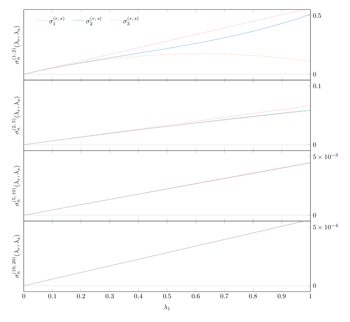
Refer to caption
Fig. 38: Slope of the phase solution with two different oscillating modes, r𝑟r and s𝑠s, for several different combinations of the mode numbers, and for 0λr,λs1formulae-sequence0subscript𝜆𝑟subscript𝜆𝑠10\leq\lambda_{r},\lambda_{s}\leq 1.

Finally, we present the third-order solution for a source equation with two distinct modes.

ϕ(3)(r,s)(x)=±π[12(λrr+λss)24(λr2r+λs2s)+14((sr)3/2(r+s)3/2)λrrλss+33116(λr3r+λs3s)\displaystyle\phi_{(3)}^{(r,s)}(x)=\pm\,\pi\!\left[\vphantom{\Bigg{[}\Bigg{]}^{\!\!\!2\,}}\frac{1}{2}\!\left(\!\frac{\lambda_{r}}{\sqrt{r}}+\frac{\lambda_{s}}{\sqrt{s}}\!\right)\!-\frac{\sqrt{2}}{4}\!\left(\vphantom{\Bigg{[}\Bigg{]}}\!\frac{\lambda_{r}^{2}}{\sqrt{r}}+\frac{\lambda_{s}^{2}}{\sqrt{s}}\!\right)\!+\frac{1}{4}\!\left(\left(s-r\right)^{\nicefrac{{3}}{{2}}}-\left(r+s\right)^{\nicefrac{{3}}{{2}}}\right)\!\frac{\lambda_{r}}{r}\frac{\lambda_{s}}{s}+\frac{3\sqrt{3}-1}{16}\!\left(\vphantom{\Bigg{[}\Bigg{]}}\!\frac{\lambda_{r}^{3}}{\sqrt{r}}+\frac{\lambda_{s}^{3}}{\sqrt{s}}\!\right)\right.
+116((2r+s)5/2sgn(2rs)|2rs|5/22s5/2)λr2r2λss+116((2s+r)5/2(2sr)5/22r5/2)λrrλs2s2]\StrLen[\arglen]([xπ])\displaystyle\quad\quad\left.\vphantom{\Bigg{[}\Bigg{]}^{\!\!\!2\,}}+\frac{1}{16}\!\left(\left(2r+s\right)^{\nicefrac{{5}}{{2}}}\!-\mathop{}\!\mathrm{sgn}(2r-s)\!\left|2r-s\right|^{\nicefrac{{5}}{{2}}}\!-2s^{\nicefrac{{5}}{{2}}}\right)\!\frac{\lambda_{r}^{2}}{r^{2}}\frac{\lambda_{s}}{s}+\frac{1}{16}\!\left(\left(2s+r\right)^{\nicefrac{{5}}{{2}}}\!-\left(2s-r\right)^{\nicefrac{{5}}{{2}}}\!-2r^{\nicefrac{{5}}{{2}}}\right)\!\frac{\lambda_{r}}{r}\frac{\lambda_{s}^{2}}{s^{2}}\right]\!\!\StrLen{}[\arglen]\left(\vphantom{\left[\frac{x}{\sqrt{\pi}}\right]^{\!\!\!2\,}}\!\!\sqrt{\vphantom{|}}\!\left[\frac{x}{\sqrt{\pi}}\right]\!\right)
+π[18(λrr+λss)228(λrr+λss)(λr2r+λs2s)+18(λrr+λss)((sr)3/2(r+s)3/2)λrrλss]𝜋delimited-[]18superscriptsubscript𝜆𝑟𝑟subscript𝜆𝑠𝑠228subscript𝜆𝑟𝑟subscript𝜆𝑠𝑠superscriptsubscript𝜆𝑟2𝑟superscriptsubscript𝜆𝑠2𝑠18subscript𝜆𝑟𝑟subscript𝜆𝑠𝑠superscript𝑠𝑟32superscript𝑟𝑠32subscript𝜆𝑟𝑟subscript𝜆𝑠𝑠\displaystyle\quad\quad\quad\quad\quad\quad\quad+\pi\!\left[\vphantom{\Bigg{[}\Bigg{]}^{\!\!\!2\,}}\frac{1}{8}\!\left(\!\frac{\lambda_{r}}{\sqrt{r}}+\frac{\lambda_{s}}{\sqrt{s}}\!\right)^{\!\!\!2\,}\!-\frac{\sqrt{2}}{8}\!\left(\!\frac{\lambda_{r}}{\sqrt{r}}+\frac{\lambda_{s}}{\sqrt{s}}\!\right)\!\!\left(\vphantom{\Bigg{[}\Bigg{]}}\!\frac{\lambda_{r}^{2}}{\sqrt{r}}+\frac{\lambda_{s}^{2}}{\sqrt{s}}\!\right)\!+\frac{1}{8}\!\left(\!\frac{\lambda_{r}}{\sqrt{r}}+\frac{\lambda_{s}}{\sqrt{s}}\!\right)\!\!\left(\left(s-r\right)^{\nicefrac{{3}}{{2}}}-\left(r+s\right)^{\nicefrac{{3}}{{2}}}\right)\!\frac{\lambda_{r}}{r}\frac{\lambda_{s}}{s}\right]
+π(λrr\StrLenr[\arglen](r[xπ±σ2(r,s)])(C\StrLenr[\arglen](r[xπ±σ2(r,s)])12)\displaystyle\quad\quad+\pi\!\left(\vphantom{\left[\Bigg{[}\Bigg{]}^{\!\!\!2\,}\right]^{\!\!\!2\,}}\frac{\lambda_{r}}{r}\!\StrLen{r}[\arglen]\left(\vphantom{\left[\frac{x}{\sqrt{\pi}}\pm\sigma_{2}^{(r,\,s)}\right]^{\!\!\!2\,}}\!\!\sqrt{\vphantom{|}r}\!\left[\frac{x}{\sqrt{\pi}}\pm\sigma_{2}^{(r,\,s)}\right]\!\right)\!\!\left(\!\vphantom{\left[\left[\frac{x}{\sqrt{\pi}}r\pm\sigma_{2}^{(r,\,s)}\right]^{\!\!\!2\,}\right]^{\!\!\!2\,}}C\!\StrLen{r}[\arglen]\left(\vphantom{\left[\frac{x}{\sqrt{\pi}}\pm\sigma_{2}^{(r,\,s)}\right]^{\!\!\!2\,}}\!\!\sqrt{\vphantom{|}r}\!\left[\frac{x}{\sqrt{\pi}}\pm\sigma_{2}^{(r,\,s)}\right]\!\right)\!\mp\frac{1}{2}\!\right)\right.
+λss\StrLens[\arglen](s[xπ±σ2(r,s)])(C\StrLens[\arglen](s[xπ±σ2(r,s)])12))\displaystyle\quad\quad\quad\quad\quad\quad\quad\quad\quad\quad\quad\quad\quad\quad\quad\quad\quad\quad\quad\quad\quad\quad\quad\quad\quad\;\;\left.+\,\frac{\lambda_{s}}{s}\StrLen{s}[\arglen]\left(\vphantom{\left[\frac{x}{\sqrt{\pi}}\pm\sigma_{2}^{(r,\,s)}\right]^{\!\!\!2\,}}\!\!\sqrt{\vphantom{|}s}\!\left[\frac{x}{\sqrt{\pi}}\pm\sigma_{2}^{(r,\,s)}\right]\!\right)\!\!\left(\!\vphantom{\left[\left[\frac{x}{\sqrt{\pi}}s\pm\sigma_{2}^{(r,\,s)}\right]^{\!\!\!2\,}\right]^{\!\!\!2\,}}C\!\StrLen{s}[\arglen]\left(\vphantom{\left[\frac{x}{\sqrt{\pi}}\pm\sigma_{2}^{(r,\,s)}\right]^{\!\!\!2\,}}\!\!\sqrt{\vphantom{|}s}\!\left[\frac{x}{\sqrt{\pi}}\pm\sigma_{2}^{(r,\,s)}\right]\!\right)\!\mp\frac{1}{2}\!\right)\!\!\right)
λrrsin[π2\StrLenr[\arglen](r[xπ±σ2(r,s)])2]λsssin[π2\StrLens[\arglen](s[xπ±σ2(r,s)])2]subscript𝜆𝑟𝑟𝜋2\StrLen𝑟delimited-[]\arglensuperscript𝑟delimited-[]plus-or-minus𝑥𝜋superscriptsubscript𝜎2𝑟𝑠2subscript𝜆𝑠𝑠𝜋2\StrLen𝑠delimited-[]\arglensuperscript𝑠delimited-[]plus-or-minus𝑥𝜋superscriptsubscript𝜎2𝑟𝑠2\displaystyle\quad\quad\quad\quad\quad\quad-\frac{\lambda_{r}}{r}\,\sin\!\left[\frac{\pi}{2}\!\StrLen{r}[\arglen]\left(\vphantom{\left[\frac{x}{\sqrt{\pi}}\pm\sigma_{2}^{(r,\,s)}\right]^{\!\!\!2\,}}\!\!\sqrt{\vphantom{|}r}\!\left[\frac{x}{\sqrt{\pi}}\pm\sigma_{2}^{(r,\,s)}\right]\!\right)^{\!\!\!2\,}\!\right]\!-\frac{\lambda_{s}}{s}\,\sin\!\left[\frac{\pi}{2}\!\StrLen{s}[\arglen]\left(\vphantom{\left[\frac{x}{\sqrt{\pi}}\pm\sigma_{2}^{(r,\,s)}\right]^{\!\!\!2\,}}\!\!\sqrt{\vphantom{|}s}\!\left[\frac{x}{\sqrt{\pi}}\pm\sigma_{2}^{(r,\,s)}\right]\!\right)^{\!\!\!2\,}\!\right]
+π2(λrr(C\StrLenr[\arglen](r[xπ±σ1(r,s)])12)+λss(C\StrLens[\arglen](s[xπ±σ1(r,s)])12))2𝜋2superscriptsubscript𝜆𝑟𝑟minus-or-plus𝐶\StrLen𝑟delimited-[]\arglen𝑟delimited-[]plus-or-minus𝑥𝜋superscriptsubscript𝜎1𝑟𝑠12subscript𝜆𝑠𝑠minus-or-plus𝐶\StrLen𝑠delimited-[]\arglen𝑠delimited-[]plus-or-minus𝑥𝜋superscriptsubscript𝜎1𝑟𝑠122\displaystyle\quad\quad+\frac{\pi}{2}\!\left(\vphantom{\left[\Bigg{[}\Bigg{]}^{\!\!\!2\,}\right]^{\!\!\!2\,}}\!\frac{\lambda_{r}}{\sqrt{r}}\!\left(\!\vphantom{\left[\left[\frac{x}{\sqrt{\pi}}r\pm\sigma_{1}^{(r,\,s)}\right]^{\!\!\!2\,}\right]^{\!\!\!2\,}}C\!\StrLen{r}[\arglen]\left(\vphantom{\left[\frac{x}{\sqrt{\pi}}\pm\sigma_{1}^{(r,\,s)}\right]^{\!\!\!2\,}}\!\!\sqrt{\vphantom{|}r}\!\left[\frac{x}{\sqrt{\pi}}\pm\sigma_{1}^{(r,\,s)}\right]\!\right)\!\mp\frac{1}{2}\!\right)\!+\frac{\lambda_{s}}{\sqrt{s}}\!\left(\!\vphantom{\left[\left[\frac{x}{\sqrt{\pi}}s\pm\sigma_{1}^{(r,\,s)}\right]^{\!\!\!2\,}\right]^{\!\!\!2\,}}C\!\StrLen{s}[\arglen]\left(\vphantom{\left[\frac{x}{\sqrt{\pi}}\pm\sigma_{1}^{(r,\,s)}\right]^{\!\!\!2\,}}\!\!\sqrt{\vphantom{|}s}\!\left[\frac{x}{\sqrt{\pi}}\pm\sigma_{1}^{(r,\,s)}\right]\!\right)\!\mp\frac{1}{2}\!\right)\!\!\right)^{\!\!\!2\,}
+π2λrrλss((sr)\StrLensr[\arglen](sr[xπ±σ1(r,s)])(C\StrLensr[\arglen](sr[xπ±σ1(r,s)])12)\displaystyle\quad\quad+\frac{\pi}{2}\,\frac{\lambda_{r}}{r}\frac{\lambda_{s}}{s}\!\left(\!\left(s-r\right)\!\StrLen{s-r}[\arglen]\left(\vphantom{\left[\frac{x}{\sqrt{\pi}}\pm\sigma_{1}^{(r,\,s)}\right]^{\!\!\!2\,}}\!\!\sqrt{\vphantom{|}s-r}\!\left[\frac{x}{\sqrt{\pi}}\pm\sigma_{1}^{(r,\,s)}\right]\!\right)\!\!\left(\!\vphantom{\left[\left[\frac{x}{\sqrt{\pi}}s-r\pm\sigma_{1}^{(r,\,s)}\right]^{\!\!\!2\,}\right]^{\!\!\!2\,}}C\!\StrLen{s-r}[\arglen]\left(\vphantom{\left[\frac{x}{\sqrt{\pi}}\pm\sigma_{1}^{(r,\,s)}\right]^{\!\!\!2\,}}\!\!\sqrt{\vphantom{|}s-r}\!\left[\frac{x}{\sqrt{\pi}}\pm\sigma_{1}^{(r,\,s)}\right]\!\right)\!\mp\frac{1}{2}\!\right)\vphantom{\left[\Bigg{[}\Bigg{]}^{\!\!\!2\,}\right]^{\!\!\!2\,}}\right.
(r+s)\StrLenr+s[\arglen](r+s[xπ±σ1(r,s)])(C\StrLenr+s[\arglen](r+s[xπ±σ1(r,s)])12))\displaystyle\quad\quad\quad\quad\quad\quad\quad\quad\quad\quad\quad\quad\quad\quad\quad\quad\quad\quad\quad\quad\left.\vphantom{\left[\Bigg{[}\Bigg{]}^{\!\!\!2\,}\right]^{\!\!\!2\,}}-\left(r+s\right)\!\StrLen{r+s}[\arglen]\left(\vphantom{\left[\frac{x}{\sqrt{\pi}}\pm\sigma_{1}^{(r,\,s)}\right]^{\!\!\!2\,}}\!\!\sqrt{\vphantom{|}r+s}\!\left[\frac{x}{\sqrt{\pi}}\pm\sigma_{1}^{(r,\,s)}\right]\!\right)\!\!\left(\!\vphantom{\left[\left[\frac{x}{\sqrt{\pi}}r+s\pm\sigma_{1}^{(r,\,s)}\right]^{\!\!\!2\,}\right]^{\!\!\!2\,}}C\!\StrLen{r+s}[\arglen]\left(\vphantom{\left[\frac{x}{\sqrt{\pi}}\pm\sigma_{1}^{(r,\,s)}\right]^{\!\!\!2\,}}\!\!\sqrt{\vphantom{|}r+s}\!\left[\frac{x}{\sqrt{\pi}}\pm\sigma_{1}^{(r,\,s)}\right]\!\right)\!\mp\frac{1}{2}\!\right)\!\!\right)
π2(λr2r\StrLen2r[\arglen](2r[xπ±σ1(r,s)])(C\StrLen2r[\arglen](2r[xπ±σ1(r,s)])12)\displaystyle\quad\quad-\frac{\pi}{2}\!\left(\vphantom{\left[\Bigg{[}\Bigg{]}^{\!\!\!2\,}\right]^{\!\!\!2\,}}\!\frac{\lambda_{r}^{2}}{r}\StrLen{2r}[\arglen]\left(\vphantom{\left[\frac{x}{\sqrt{\pi}}\pm\sigma_{1}^{(r,\,s)}\right]^{\!\!\!2\,}}\!\!\sqrt{\vphantom{|}2r}\!\left[\frac{x}{\sqrt{\pi}}\pm\sigma_{1}^{(r,\,s)}\right]\!\right)\!\!\left(\!\vphantom{\left[\left[\frac{x}{\sqrt{\pi}}2r\pm\sigma_{1}^{(r,\,s)}\right]^{\!\!\!2\,}\right]^{\!\!\!2\,}}C\!\StrLen{2r}[\arglen]\left(\vphantom{\left[\frac{x}{\sqrt{\pi}}\pm\sigma_{1}^{(r,\,s)}\right]^{\!\!\!2\,}}\!\!\sqrt{\vphantom{|}2r}\!\left[\frac{x}{\sqrt{\pi}}\pm\sigma_{1}^{(r,\,s)}\right]\!\right)\!\mp\frac{1}{2}\!\right)\right.
+λs2s\StrLen2s[\arglen](2s[xπ±σ1(r,s)])(C\StrLen2s[\arglen](2s[xπ±σ1(r,s)])12))\displaystyle\quad\quad\quad\quad\quad\quad\quad\quad\quad\quad\quad\quad\quad\quad\quad\quad\quad\quad\quad\quad\quad\quad\quad\quad\left.+\frac{\lambda_{s}^{2}}{s}\StrLen{2s}[\arglen]\left(\vphantom{\left[\frac{x}{\sqrt{\pi}}\pm\sigma_{1}^{(r,\,s)}\right]^{\!\!\!2\,}}\!\!\sqrt{\vphantom{|}2s}\!\left[\frac{x}{\sqrt{\pi}}\pm\sigma_{1}^{(r,\,s)}\right]\!\right)\!\!\left(\!\vphantom{\left[\left[\frac{x}{\sqrt{\pi}}2s\pm\sigma_{1}^{(r,\,s)}\right]^{\!\!\!2\,}\right]^{\!\!\!2\,}}C\!\StrLen{2s}[\arglen]\left(\vphantom{\left[\frac{x}{\sqrt{\pi}}\pm\sigma_{1}^{(r,\,s)}\right]^{\!\!\!2\,}}\!\!\sqrt{\vphantom{|}2s}\!\left[\frac{x}{\sqrt{\pi}}\pm\sigma_{1}^{(r,\,s)}\right]\!\right)\!\mp\frac{1}{2}\!\right)\!\!\right)
12λrrλss((sr)sin[π2\StrLensr[\arglen](sr[xπ±σ1(r,s)])2](r+s)sin[π2\StrLenr+s[\arglen](r+s[xπ±σ1(r,s)])2])12subscript𝜆𝑟𝑟subscript𝜆𝑠𝑠𝑠𝑟𝜋2\StrLen𝑠𝑟delimited-[]\arglensuperscript𝑠𝑟delimited-[]plus-or-minus𝑥𝜋superscriptsubscript𝜎1𝑟𝑠2𝑟𝑠𝜋2\StrLen𝑟𝑠delimited-[]\arglensuperscript𝑟𝑠delimited-[]plus-or-minus𝑥𝜋superscriptsubscript𝜎1𝑟𝑠2\displaystyle\quad\quad\quad\quad\quad\quad-\frac{1}{2}\,\frac{\lambda_{r}}{r}\frac{\lambda_{s}}{s}\!\left(\vphantom{\left[\Bigg{[}\Bigg{]}^{\!\!\!2\,}\right]^{\!\!\!2\,}}\!\!\left(s-r\right)\,\sin\!\left[\frac{\pi}{2}\!\StrLen{s-r}[\arglen]\left(\vphantom{\left[\frac{x}{\sqrt{\pi}}\pm\sigma_{1}^{(r,\,s)}\right]^{\!\!\!2\,}}\!\!\sqrt{\vphantom{|}s-r}\!\left[\frac{x}{\sqrt{\pi}}\pm\sigma_{1}^{(r,\,s)}\right]\!\right)^{\!\!\!2\,}\!\right]\!-\left(r+s\right)\,\sin\!\left[\frac{\pi}{2}\!\StrLen{r+s}[\arglen]\left(\vphantom{\left[\frac{x}{\sqrt{\pi}}\pm\sigma_{1}^{(r,\,s)}\right]^{\!\!\!2\,}}\!\!\sqrt{\vphantom{|}r+s}\!\left[\frac{x}{\sqrt{\pi}}\pm\sigma_{1}^{(r,\,s)}\right]\!\right)^{\!\!\!2\,}\!\right]\!\right)
+12(λr2rsin[π2\StrLen2r[\arglen](2r[xπ±σ1(r,s)])2]+λs2ssin[π2\StrLen2s[\arglen](2s[xπ±σ1(r,s)])2])12superscriptsubscript𝜆𝑟2𝑟𝜋2\StrLen2𝑟delimited-[]\arglensuperscript2𝑟delimited-[]plus-or-minus𝑥𝜋superscriptsubscript𝜎1𝑟𝑠2superscriptsubscript𝜆𝑠2𝑠𝜋2\StrLen2𝑠delimited-[]\arglensuperscript2𝑠delimited-[]plus-or-minus𝑥𝜋superscriptsubscript𝜎1𝑟𝑠2\displaystyle\quad\quad\quad\quad\quad\quad\quad\quad\quad\quad+\frac{1}{2}\!\left(\vphantom{\left[\Bigg{[}\Bigg{]}^{\!\!\!2\,}\right]^{\!\!\!2\,}}\!\frac{\lambda_{r}^{2}}{r}\,\sin\!\left[\frac{\pi}{2}\!\StrLen{2r}[\arglen]\left(\vphantom{\left[\frac{x}{\sqrt{\pi}}\pm\sigma_{1}^{(r,\,s)}\right]^{\!\!\!2\,}}\!\!\sqrt{\vphantom{|}2r}\!\left[\frac{x}{\sqrt{\pi}}\pm\sigma_{1}^{(r,\,s)}\right]\!\right)^{\!\!\!2\,}\!\right]\!+\frac{\lambda_{s}^{2}}{s}\,\sin\!\left[\frac{\pi}{2}\!\StrLen{2s}[\arglen]\left(\vphantom{\left[\frac{x}{\sqrt{\pi}}\pm\sigma_{1}^{(r,\,s)}\right]^{\!\!\!2\,}}\!\!\sqrt{\vphantom{|}2s}\!\left[\frac{x}{\sqrt{\pi}}\pm\sigma_{1}^{(r,\,s)}\right]\!\right)^{\!\!\!2\,}\!\right]\!\right)
+π2(λrcos[π2\StrLenr[\arglen](r[xπ])2]+λscos[π2\StrLens[\arglen](s[xπ])2])(λrr(C\StrLenr[\arglen](r[xπ])12)+λss(C\StrLens[\arglen](s[xπ])12))2𝜋2subscript𝜆𝑟𝜋2\StrLen𝑟delimited-[]\arglensuperscript𝑟delimited-[]𝑥𝜋2subscript𝜆𝑠𝜋2\StrLen𝑠delimited-[]\arglensuperscript𝑠delimited-[]𝑥𝜋2superscriptsubscript𝜆𝑟𝑟minus-or-plus𝐶\StrLen𝑟delimited-[]\arglen𝑟delimited-[]𝑥𝜋12subscript𝜆𝑠𝑠minus-or-plus𝐶\StrLen𝑠delimited-[]\arglen𝑠delimited-[]𝑥𝜋122\displaystyle\quad\quad+\frac{\pi}{2}\!\left(\vphantom{\left[\Bigg{[}\Bigg{]}^{\!\!\!2\,}\right]^{\!\!\!2\,}}\!\lambda_{r}\,\cos\!\left[\frac{\pi}{2}\!\StrLen{r}[\arglen]\left(\vphantom{\left[\frac{x}{\sqrt{\pi}}\right]^{\!\!\!2\,}}\!\!\sqrt{\vphantom{|}r}\!\left[\frac{x}{\sqrt{\pi}}\right]\!\right)^{\!\!\!2\,}\!\right]\!+\lambda_{s}\,\cos\!\left[\frac{\pi}{2}\!\StrLen{s}[\arglen]\left(\vphantom{\left[\frac{x}{\sqrt{\pi}}\right]^{\!\!\!2\,}}\!\!\sqrt{\vphantom{|}s}\!\left[\frac{x}{\sqrt{\pi}}\right]\!\right)^{\!\!\!2\,}\!\right]\!\right)\!\!\left(\vphantom{\left[\Bigg{[}\Bigg{]}^{\!\!\!2\,}\right]^{\!\!\!2\,}}\!\frac{\lambda_{r}}{\sqrt{r}}\!\left(\!\vphantom{\left[\left[\frac{x}{\sqrt{\pi}}r\right]^{\!\!\!2\,}\right]^{\!\!\!2\,}}C\!\StrLen{r}[\arglen]\left(\vphantom{\left[\frac{x}{\sqrt{\pi}}\right]^{\!\!\!2\,}}\!\!\sqrt{\vphantom{|}r}\!\left[\frac{x}{\sqrt{\pi}}\right]\!\right)\!\mp\frac{1}{2}\!\right)\!+\frac{\lambda_{s}}{\sqrt{s}}\!\left(\!\vphantom{\left[\left[\frac{x}{\sqrt{\pi}}s\right]^{\!\!\!2\,}\right]^{\!\!\!2\,}}C\!\StrLen{s}[\arglen]\left(\vphantom{\left[\frac{x}{\sqrt{\pi}}\right]^{\!\!\!2\,}}\!\!\sqrt{\vphantom{|}s}\!\left[\frac{x}{\sqrt{\pi}}\right]\!\right)\!\mp\frac{1}{2}\!\right)\!\!\right)^{\!\!\!2\,}
+π2λrrλss((sr)3/2(C\StrLensr[\arglen](sr[xπ])12)(r+s)3/2(C\StrLenr+s[\arglen](r+s[xπ])12))×\displaystyle\quad\quad+\frac{\pi}{2}\,\frac{\lambda_{r}}{r}\frac{\lambda_{s}}{s}\!\left(\vphantom{\left[\Bigg{[}\Bigg{]}^{\!\!\!2\,}\right]^{\!\!\!2\,}}\!\!\left(s-r\right)^{\nicefrac{{3}}{{2}}}\!\left(\!\vphantom{\left[\left[\frac{x}{\sqrt{\pi}}s-r\right]^{\!\!\!2\,}\right]^{\!\!\!2\,}}C\!\StrLen{s-r}[\arglen]\left(\vphantom{\left[\frac{x}{\sqrt{\pi}}\right]^{\!\!\!2\,}}\!\!\sqrt{\vphantom{|}s-r}\!\left[\frac{x}{\sqrt{\pi}}\right]\!\right)\!\mp\frac{1}{2}\!\right)\!-\left(r+s\right)^{\nicefrac{{3}}{{2}}}\!\left(\!\vphantom{\left[\left[\frac{x}{\sqrt{\pi}}r+s\right]^{\!\!\!2\,}\right]^{\!\!\!2\,}}C\!\StrLen{r+s}[\arglen]\left(\vphantom{\left[\frac{x}{\sqrt{\pi}}\right]^{\!\!\!2\,}}\!\!\sqrt{\vphantom{|}r+s}\!\left[\frac{x}{\sqrt{\pi}}\right]\!\right)\!\mp\frac{1}{2}\!\right)\!\!\right)\!\times
×(λrr(C\StrLenr[\arglen](r[xπ])12)+λss(C\StrLens[\arglen](s[xπ])12))absentsubscript𝜆𝑟𝑟minus-or-plus𝐶\StrLen𝑟delimited-[]\arglen𝑟delimited-[]𝑥𝜋12subscript𝜆𝑠𝑠minus-or-plus𝐶\StrLen𝑠delimited-[]\arglen𝑠delimited-[]𝑥𝜋12\displaystyle\quad\quad\quad\quad\quad\quad\quad\quad\quad\quad\quad\quad\quad\quad\quad\quad\quad\quad\quad\quad\quad\quad\quad\quad\quad\times\!\left(\vphantom{\left[\Bigg{[}\Bigg{]}^{\!\!\!2\,}\right]^{\!\!\!2\,}}\!\frac{\lambda_{r}}{\sqrt{r}}\!\left(\!\vphantom{\left[\left[\frac{x}{\sqrt{\pi}}r\right]^{\!\!\!2\,}\right]^{\!\!\!2\,}}C\!\StrLen{r}[\arglen]\left(\vphantom{\left[\frac{x}{\sqrt{\pi}}\right]^{\!\!\!2\,}}\!\!\sqrt{\vphantom{|}r}\!\left[\frac{x}{\sqrt{\pi}}\right]\!\right)\!\mp\frac{1}{2}\!\right)\!+\frac{\lambda_{s}}{\sqrt{s}}\!\left(\!\vphantom{\left[\left[\frac{x}{\sqrt{\pi}}s\right]^{\!\!\!2\,}\right]^{\!\!\!2\,}}C\!\StrLen{s}[\arglen]\left(\vphantom{\left[\frac{x}{\sqrt{\pi}}\right]^{\!\!\!2\,}}\!\!\sqrt{\vphantom{|}s}\!\left[\frac{x}{\sqrt{\pi}}\right]\!\right)\!\mp\frac{1}{2}\!\right)\!\!\right)
π2(λr2r(C\StrLen2r[\arglen](2r[xπ])12)+λs2s(C\StrLen2s[\arglen](2s[xπ])12))×\displaystyle\quad\quad-\frac{\pi}{\sqrt{2}}\!\left(\vphantom{\left[\Bigg{[}\Bigg{]}^{\!\!\!2\,}\right]^{\!\!\!2\,}}\!\frac{\lambda_{r}^{2}}{\sqrt{r}}\!\left(\!\vphantom{\left[\left[\frac{x}{\sqrt{\pi}}2r\right]^{\!\!\!2\,}\right]^{\!\!\!2\,}}C\!\StrLen{2r}[\arglen]\left(\vphantom{\left[\frac{x}{\sqrt{\pi}}\right]^{\!\!\!2\,}}\!\!\sqrt{\vphantom{|}2r}\!\left[\frac{x}{\sqrt{\pi}}\right]\!\right)\!\mp\frac{1}{2}\!\right)\!+\frac{\lambda_{s}^{2}}{\sqrt{s}}\!\left(\!\vphantom{\left[\left[\frac{x}{\sqrt{\pi}}2s\right]^{\!\!\!2\,}\right]^{\!\!\!2\,}}C\!\StrLen{2s}[\arglen]\left(\vphantom{\left[\frac{x}{\sqrt{\pi}}\right]^{\!\!\!2\,}}\!\!\sqrt{\vphantom{|}2s}\!\left[\frac{x}{\sqrt{\pi}}\right]\!\right)\!\mp\frac{1}{2}\!\right)\!\!\right)\!\times
×(λrr(C\StrLenr[\arglen](r[xπ])12)+λss(C\StrLens[\arglen](s[xπ])12))absentsubscript𝜆𝑟𝑟minus-or-plus𝐶\StrLen𝑟delimited-[]\arglen𝑟delimited-[]𝑥𝜋12subscript𝜆𝑠𝑠minus-or-plus𝐶\StrLen𝑠delimited-[]\arglen𝑠delimited-[]𝑥𝜋12\displaystyle\quad\quad\quad\quad\quad\quad\quad\quad\quad\quad\quad\quad\quad\quad\quad\quad\quad\quad\quad\quad\quad\quad\quad\quad\quad\times\!\left(\vphantom{\left[\Bigg{[}\Bigg{]}^{\!\!\!2\,}\right]^{\!\!\!2\,}}\!\frac{\lambda_{r}}{\sqrt{r}}\!\left(\!\vphantom{\left[\left[\frac{x}{\sqrt{\pi}}r\right]^{\!\!\!2\,}\right]^{\!\!\!2\,}}C\!\StrLen{r}[\arglen]\left(\vphantom{\left[\frac{x}{\sqrt{\pi}}\right]^{\!\!\!2\,}}\!\!\sqrt{\vphantom{|}r}\!\left[\frac{x}{\sqrt{\pi}}\right]\!\right)\!\mp\frac{1}{2}\!\right)\!+\frac{\lambda_{s}}{\sqrt{s}}\!\left(\!\vphantom{\left[\left[\frac{x}{\sqrt{\pi}}s\right]^{\!\!\!2\,}\right]^{\!\!\!2\,}}C\!\StrLen{s}[\arglen]\left(\vphantom{\left[\frac{x}{\sqrt{\pi}}\right]^{\!\!\!2\,}}\!\!\sqrt{\vphantom{|}s}\!\left[\frac{x}{\sqrt{\pi}}\right]\!\right)\!\mp\frac{1}{2}\!\right)\!\!\right)\!\!
+3π8(λr3r\StrLen3r[\arglen](3r[xπ])(C\StrLen3r[\arglen](3r[xπ])12)+λs3s\StrLen3s[\arglen](3s[xπ])(C\StrLen3s[\arglen](3s[xπ])12))3𝜋8superscriptsubscript𝜆𝑟3𝑟\StrLen3𝑟delimited-[]\arglen3𝑟delimited-[]𝑥𝜋minus-or-plus𝐶\StrLen3𝑟delimited-[]\arglen3𝑟delimited-[]𝑥𝜋12superscriptsubscript𝜆𝑠3𝑠\StrLen3𝑠delimited-[]\arglen3𝑠delimited-[]𝑥𝜋minus-or-plus𝐶\StrLen3𝑠delimited-[]\arglen3𝑠delimited-[]𝑥𝜋12\displaystyle\quad\quad+\frac{3\pi}{8}\!\left(\vphantom{\left[\Bigg{[}\Bigg{]}^{\!\!\!2\,}\right]^{\!\!\!2\,}}\!\frac{\lambda_{r}^{3}}{r}\!\StrLen{3r}[\arglen]\left(\vphantom{\left[\frac{x}{\sqrt{\pi}}\right]^{\!\!\!2\,}}\!\!\sqrt{\vphantom{|}3r}\!\left[\frac{x}{\sqrt{\pi}}\right]\!\right)\!\!\left(\!\vphantom{\left[\left[\frac{x}{\sqrt{\pi}}3r\right]^{\!\!\!2\,}\right]^{\!\!\!2\,}}C\!\StrLen{3r}[\arglen]\left(\vphantom{\left[\frac{x}{\sqrt{\pi}}\right]^{\!\!\!2\,}}\!\!\sqrt{\vphantom{|}3r}\!\left[\frac{x}{\sqrt{\pi}}\right]\!\right)\!\mp\frac{1}{2}\!\right)\!+\frac{\lambda_{s}^{3}}{s}\!\StrLen{3s}[\arglen]\left(\vphantom{\left[\frac{x}{\sqrt{\pi}}\right]^{\!\!\!2\,}}\!\!\sqrt{\vphantom{|}3s}\!\left[\frac{x}{\sqrt{\pi}}\right]\!\right)\!\!\left(\!\vphantom{\left[\left[\frac{x}{\sqrt{\pi}}3s\right]^{\!\!\!2\,}\right]^{\!\!\!2\,}}C\!\StrLen{3s}[\arglen]\left(\vphantom{\left[\frac{x}{\sqrt{\pi}}\right]^{\!\!\!2\,}}\!\!\sqrt{\vphantom{|}3s}\!\left[\frac{x}{\sqrt{\pi}}\right]\!\right)\!\mp\frac{1}{2}\!\right)\!\!\right)
+π8λrrλss(λrr(2r+s)2\StrLen2r+s[\arglen](2r+s[xπ])(C\StrLen2r+s[\arglen](2r+s[xπ])12)\displaystyle\quad\quad+\frac{\pi}{8}\,\frac{\lambda_{r}}{r}\frac{\lambda_{s}}{s}\!\left(\!\frac{\lambda_{r}}{r}\left(2r+s\right)^{2}\!\StrLen{2r+s}[\arglen]\left(\vphantom{\left[\frac{x}{\sqrt{\pi}}\right]^{\!\!\!2\,}}\!\!\sqrt{\vphantom{|}2r+s}\!\left[\frac{x}{\sqrt{\pi}}\right]\!\right)\!\!\left(\!\vphantom{\left[\left[\frac{x}{\sqrt{\pi}}2r+s\right]^{\!\!\!2\,}\right]^{\!\!\!2\,}}C\!\StrLen{2r+s}[\arglen]\left(\vphantom{\left[\frac{x}{\sqrt{\pi}}\right]^{\!\!\!2\,}}\!\!\sqrt{\vphantom{|}2r+s}\!\left[\frac{x}{\sqrt{\pi}}\right]\!\right)\!\mp\frac{1}{2}\!\right)\vphantom{\left[\Bigg{[}\Bigg{]}^{\!\!\!2\,}\right]^{\!\!\!2\,}}\right.
+λss(2s+r)2\StrLen2s+r[\arglen](2s+r[xπ])(C\StrLen2s+r[\arglen](2s+r[xπ])12))\displaystyle\quad\quad\quad\quad\quad\quad\quad\quad\quad\quad\quad\quad\quad\quad\quad\quad\quad\quad\quad\quad\quad\quad\quad\left.\vphantom{\left[\Bigg{[}\Bigg{]}^{\!\!\!2\,}\right]^{\!\!\!2\,}}+\frac{\lambda_{s}}{s}\left(2s+r\right)^{2}\!\StrLen{2s+r}[\arglen]\left(\vphantom{\left[\frac{x}{\sqrt{\pi}}\right]^{\!\!\!2\,}}\!\!\sqrt{\vphantom{|}2s+r}\!\left[\frac{x}{\sqrt{\pi}}\right]\!\right)\!\!\left(\!\vphantom{\left[\left[\frac{x}{\sqrt{\pi}}2s+r\right]^{\!\!\!2\,}\right]^{\!\!\!2\,}}C\!\StrLen{2s+r}[\arglen]\left(\vphantom{\left[\frac{x}{\sqrt{\pi}}\right]^{\!\!\!2\,}}\!\!\sqrt{\vphantom{|}2s+r}\!\left[\frac{x}{\sqrt{\pi}}\right]\!\right)\!\mp\frac{1}{2}\!\right)\!\!\right)
π8λrrλss(λrrsgn(2rs)(2rs)2\StrLen|2rs|[\arglen](|2rs|[xπ])(C\StrLen|2rs|[\arglen](|2rs|[xπ])12)\displaystyle\quad\quad-\frac{\pi}{8}\,\frac{\lambda_{r}}{r}\frac{\lambda_{s}}{s}\!\left(\!\frac{\lambda_{r}}{r}\mathop{}\!\mathrm{sgn}(2r-s)\left(2r-s\right)^{2}\!\StrLen{|2r-s|}[\arglen]\left(\vphantom{\left[\frac{x}{\sqrt{\pi}}\right]^{\!\!\!2\,}}\!\!\sqrt{\vphantom{|}|2r-s|}\!\left[\frac{x}{\sqrt{\pi}}\right]\!\right)\!\!\left(\!\vphantom{\left[\left[\frac{x}{\sqrt{\pi}}|2r-s|\right]^{\!\!\!2\,}\right]^{\!\!\!2\,}}C\!\StrLen{|2r-s|}[\arglen]\left(\vphantom{\left[\frac{x}{\sqrt{\pi}}\right]^{\!\!\!2\,}}\!\!\sqrt{\vphantom{|}|2r-s|}\!\left[\frac{x}{\sqrt{\pi}}\right]\!\right)\!\mp\frac{1}{2}\!\right)\vphantom{\left[\Bigg{[}\Bigg{]}^{\!\!\!2\,}\right]^{\!\!\!2\,}}\right.
+λss(2sr)2\StrLen2sr[\arglen](2sr[xπ])(C\StrLen2sr[\arglen](2sr[xπ])12))\displaystyle\quad\quad\quad\quad\quad\quad\quad\quad\quad\quad\quad\quad\quad\quad\quad\quad\quad\quad\quad\quad\quad\quad\quad\left.\vphantom{\left[\Bigg{[}\Bigg{]}^{\!\!\!2\,}\right]^{\!\!\!2\,}}+\,\frac{\lambda_{s}}{s}\left(2s-r\right)^{2}\!\StrLen{2s-r}[\arglen]\left(\vphantom{\left[\frac{x}{\sqrt{\pi}}\right]^{\!\!\!2\,}}\!\!\sqrt{\vphantom{|}2s-r}\!\left[\frac{x}{\sqrt{\pi}}\right]\!\right)\!\!\left(\!\vphantom{\left[\left[\frac{x}{\sqrt{\pi}}2s-r\right]^{\!\!\!2\,}\right]^{\!\!\!2\,}}C\!\StrLen{2s-r}[\arglen]\left(\vphantom{\left[\frac{x}{\sqrt{\pi}}\right]^{\!\!\!2\,}}\!\!\sqrt{\vphantom{|}2s-r}\!\left[\frac{x}{\sqrt{\pi}}\right]\!\right)\!\mp\frac{1}{2}\!\right)\!\!\right)
π8(λr3r\StrLenr[\arglen](r[xπ])(C\StrLenr[\arglen](r[xπ])12)+λs3s\StrLens[\arglen](s[xπ])(C\StrLens[\arglen](s[xπ])12))𝜋8superscriptsubscript𝜆𝑟3𝑟\StrLen𝑟delimited-[]\arglen𝑟delimited-[]𝑥𝜋minus-or-plus𝐶\StrLen𝑟delimited-[]\arglen𝑟delimited-[]𝑥𝜋12superscriptsubscript𝜆𝑠3𝑠\StrLen𝑠delimited-[]\arglen𝑠delimited-[]𝑥𝜋minus-or-plus𝐶\StrLen𝑠delimited-[]\arglen𝑠delimited-[]𝑥𝜋12\displaystyle\quad\quad-\frac{\pi}{8}\!\left(\vphantom{\left[\Bigg{[}\Bigg{]}^{\!\!\!2\,}\right]^{\!\!\!2\,}}\!\frac{\lambda_{r}^{3}}{r}\!\StrLen{r}[\arglen]\left(\vphantom{\left[\frac{x}{\sqrt{\pi}}\right]^{\!\!\!2\,}}\!\!\sqrt{\vphantom{|}r}\!\left[\frac{x}{\sqrt{\pi}}\right]\!\right)\!\!\left(\!\vphantom{\left[\left[\frac{x}{\sqrt{\pi}}r\right]^{\!\!\!2\,}\right]^{\!\!\!2\,}}C\!\StrLen{r}[\arglen]\left(\vphantom{\left[\frac{x}{\sqrt{\pi}}\right]^{\!\!\!2\,}}\!\!\sqrt{\vphantom{|}r}\!\left[\frac{x}{\sqrt{\pi}}\right]\!\right)\!\mp\frac{1}{2}\!\right)\!+\frac{\lambda_{s}^{3}}{s}\!\StrLen{s}[\arglen]\left(\vphantom{\left[\frac{x}{\sqrt{\pi}}\right]^{\!\!\!2\,}}\!\!\sqrt{\vphantom{|}s}\!\left[\frac{x}{\sqrt{\pi}}\right]\!\right)\!\!\left(\!\vphantom{\left[\left[\frac{x}{\sqrt{\pi}}s\right]^{\!\!\!2\,}\right]^{\!\!\!2\,}}C\!\StrLen{s}[\arglen]\left(\vphantom{\left[\frac{x}{\sqrt{\pi}}\right]^{\!\!\!2\,}}\!\!\sqrt{\vphantom{|}s}\!\left[\frac{x}{\sqrt{\pi}}\right]\!\right)\!\mp\frac{1}{2}\!\right)\!\!\right)
π4λrrλss(λrrs2\StrLens[\arglen](s[xπ])(C\StrLens[\arglen](s[xπ])12)+λssr2\StrLenr[\arglen](r[xπ])(C\StrLenr[\arglen](r[xπ])12))𝜋4subscript𝜆𝑟𝑟subscript𝜆𝑠𝑠subscript𝜆𝑟𝑟superscript𝑠2\StrLen𝑠delimited-[]\arglen𝑠delimited-[]𝑥𝜋minus-or-plus𝐶\StrLen𝑠delimited-[]\arglen𝑠delimited-[]𝑥𝜋12subscript𝜆𝑠𝑠superscript𝑟2\StrLen𝑟delimited-[]\arglen𝑟delimited-[]𝑥𝜋minus-or-plus𝐶\StrLen𝑟delimited-[]\arglen𝑟delimited-[]𝑥𝜋12\displaystyle\quad\quad\quad\quad\quad\quad-\frac{\pi}{4}\,\frac{\lambda_{r}}{r}\frac{\lambda_{s}}{s}\!\left(\vphantom{\left[\Bigg{[}\Bigg{]}^{\!\!\!2\,}\right]^{\!\!\!2\,}}\!\frac{\lambda_{r}}{r}\,s^{2}\!\StrLen{s}[\arglen]\left(\vphantom{\left[\frac{x}{\sqrt{\pi}}\right]^{\!\!\!2\,}}\!\!\sqrt{\vphantom{|}s}\!\left[\frac{x}{\sqrt{\pi}}\right]\!\right)\!\!\left(\!\vphantom{\left[\left[\frac{x}{\sqrt{\pi}}s\right]^{\!\!\!2\,}\right]^{\!\!\!2\,}}C\!\StrLen{s}[\arglen]\left(\vphantom{\left[\frac{x}{\sqrt{\pi}}\right]^{\!\!\!2\,}}\!\!\sqrt{\vphantom{|}s}\!\left[\frac{x}{\sqrt{\pi}}\right]\!\right)\!\mp\frac{1}{2}\!\right)\!+\frac{\lambda_{s}}{s}\,r^{2}\!\StrLen{r}[\arglen]\left(\vphantom{\left[\frac{x}{\sqrt{\pi}}\right]^{\!\!\!2\,}}\!\!\sqrt{\vphantom{|}r}\!\left[\frac{x}{\sqrt{\pi}}\right]\!\right)\!\!\left(\!\vphantom{\left[\left[\frac{x}{\sqrt{\pi}}r\right]^{\!\!\!2\,}\right]^{\!\!\!2\,}}C\!\StrLen{r}[\arglen]\left(\vphantom{\left[\frac{x}{\sqrt{\pi}}\right]^{\!\!\!2\,}}\!\!\sqrt{\vphantom{|}r}\!\left[\frac{x}{\sqrt{\pi}}\right]\!\right)\!\mp\frac{1}{2}\!\right)\!\!\right)
38(λr3rsin[π2\StrLen3r[\arglen](3r[xπ])2]+λs3ssin[π2\StrLen3s[\arglen](3s[xπ])2])38superscriptsubscript𝜆𝑟3𝑟𝜋2\StrLen3𝑟delimited-[]\arglensuperscript3𝑟delimited-[]𝑥𝜋2superscriptsubscript𝜆𝑠3𝑠𝜋2\StrLen3𝑠delimited-[]\arglensuperscript3𝑠delimited-[]𝑥𝜋2\displaystyle\quad\quad-\frac{3}{8}\!\left(\vphantom{\left[\Bigg{[}\Bigg{]}^{\!\!\!2\,}\right]^{\!\!\!2\,}}\!\frac{\lambda_{r}^{3}}{r}\,\sin\!\left[\frac{\pi}{2}\!\StrLen{3r}[\arglen]\left(\vphantom{\left[\frac{x}{\sqrt{\pi}}\right]^{\!\!\!2\,}}\!\!\sqrt{\vphantom{|}3r}\!\left[\frac{x}{\sqrt{\pi}}\right]\!\right)^{\!\!\!2\,}\!\right]\!+\frac{\lambda_{s}^{3}}{s}\,\sin\!\left[\frac{\pi}{2}\!\StrLen{3s}[\arglen]\left(\vphantom{\left[\frac{x}{\sqrt{\pi}}\right]^{\!\!\!2\,}}\!\!\sqrt{\vphantom{|}3s}\!\left[\frac{x}{\sqrt{\pi}}\right]\!\right)^{\!\!\!2\,}\!\right]\!\right)
18λrrλss(λrr(2r+s)2sin[π2\StrLen2r+s[\arglen](2r+s[xπ])2]+λss(2s+r)2sin[π2\StrLen2s+r[\arglen](2s+r[xπ])2])18subscript𝜆𝑟𝑟subscript𝜆𝑠𝑠subscript𝜆𝑟𝑟superscript2𝑟𝑠2𝜋2\StrLen2𝑟𝑠delimited-[]\arglensuperscript2𝑟𝑠delimited-[]𝑥𝜋2subscript𝜆𝑠𝑠superscript2𝑠𝑟2𝜋2\StrLen2𝑠𝑟delimited-[]\arglensuperscript2𝑠𝑟delimited-[]𝑥𝜋2\displaystyle\quad\quad\quad\quad\quad\quad-\frac{1}{8}\,\frac{\lambda_{r}}{r}\frac{\lambda_{s}}{s}\!\left(\vphantom{\left[\Bigg{[}\Bigg{]}^{\!\!\!2\,}\right]^{\!\!\!2\,}}\!\frac{\lambda_{r}}{r}\left(2r+s\right)^{2}\sin\!\left[\frac{\pi}{2}\!\StrLen{2r+s}[\arglen]\left(\vphantom{\left[\frac{x}{\sqrt{\pi}}\right]^{\!\!\!2\,}}\!\!\sqrt{\vphantom{|}2r+s}\!\left[\frac{x}{\sqrt{\pi}}\right]\!\right)^{\!\!\!2\,}\!\right]\!+\frac{\lambda_{s}}{s}\left(2s+r\right)^{2}\sin\!\left[\frac{\pi}{2}\!\StrLen{2s+r}[\arglen]\left(\vphantom{\left[\frac{x}{\sqrt{\pi}}\right]^{\!\!\!2\,}}\!\!\sqrt{\vphantom{|}2s+r}\!\left[\frac{x}{\sqrt{\pi}}\right]\!\right)^{\!\!\!2\,}\!\right]\!\right)
+18λrrλss(λrrsgn(2rs)(2rs)2sin[π2\StrLen|2rs|[\arglen](|2rs|[xπ])2]+λss(2sr)2sin[π2\StrLen2sr[\arglen](2sr[xπ])2])18subscript𝜆𝑟𝑟subscript𝜆𝑠𝑠subscript𝜆𝑟𝑟sgn2𝑟𝑠superscript2𝑟𝑠2𝜋2\StrLen2𝑟𝑠delimited-[]\arglensuperscript2𝑟𝑠delimited-[]𝑥𝜋2subscript𝜆𝑠𝑠superscript2𝑠𝑟2𝜋2\StrLen2𝑠𝑟delimited-[]\arglensuperscript2𝑠𝑟delimited-[]𝑥𝜋2\displaystyle\quad\quad\quad\quad\quad\quad+\frac{1}{8}\,\frac{\lambda_{r}}{r}\frac{\lambda_{s}}{s}\!\left(\vphantom{\left[\Bigg{[}\Bigg{]}^{\!\!\!2\,}\right]^{\!\!\!2\,}}\!\frac{\lambda_{r}}{r}\mathop{}\!\mathrm{sgn}(2r-s)\left(2r-s\right)^{2}\sin\!\left[\frac{\pi}{2}\!\StrLen{|2r-s|}[\arglen]\left(\vphantom{\left[\frac{x}{\sqrt{\pi}}\right]^{\!\!\!2\,}}\!\!\sqrt{\vphantom{|}|2r-s|}\!\left[\frac{x}{\sqrt{\pi}}\right]\!\right)^{\!\!\!2\,}\!\right]\!+\frac{\lambda_{s}}{s}\left(2s-r\right)^{2}\sin\!\left[\frac{\pi}{2}\!\StrLen{2s-r}[\arglen]\left(\vphantom{\left[\frac{x}{\sqrt{\pi}}\right]^{\!\!\!2\,}}\!\!\sqrt{\vphantom{|}2s-r}\!\left[\frac{x}{\sqrt{\pi}}\right]\!\right)^{\!\!\!2\,}\!\right]\!\right)
+18(λr3rsin[π2\StrLenr[\arglen](r[xπ])2]+λs3ssin[π2\StrLens[\arglen](s[xπ])2])18superscriptsubscript𝜆𝑟3𝑟𝜋2\StrLen𝑟delimited-[]\arglensuperscript𝑟delimited-[]𝑥𝜋2superscriptsubscript𝜆𝑠3𝑠𝜋2\StrLen𝑠delimited-[]\arglensuperscript𝑠delimited-[]𝑥𝜋2\displaystyle\quad\quad\quad\quad\quad\quad\quad\quad\quad\quad+\frac{1}{8}\!\left(\vphantom{\left[\Bigg{[}\Bigg{]}^{\!\!\!2\,}\right]^{\!\!\!2\,}}\!\frac{\lambda_{r}^{3}}{r}\,\sin\!\left[\frac{\pi}{2}\!\StrLen{r}[\arglen]\left(\vphantom{\left[\frac{x}{\sqrt{\pi}}\right]^{\!\!\!2\,}}\!\!\sqrt{\vphantom{|}r}\!\left[\frac{x}{\sqrt{\pi}}\right]\!\right)^{\!\!\!2\,}\!\right]\!+\frac{\lambda_{s}^{3}}{s}\,\sin\!\left[\frac{\pi}{2}\!\StrLen{s}[\arglen]\left(\vphantom{\left[\frac{x}{\sqrt{\pi}}\right]^{\!\!\!2\,}}\!\!\sqrt{\vphantom{|}s}\!\left[\frac{x}{\sqrt{\pi}}\right]\!\right)^{\!\!\!2\,}\!\right]\!\right)
+14λrrλss(λrsr2sin[π2\StrLenr[\arglen](r[xπ])2]+λsrs2sin[π2\StrLens[\arglen](s[xπ])2])14subscript𝜆𝑟𝑟subscript𝜆𝑠𝑠subscript𝜆𝑟𝑠superscript𝑟2𝜋2\StrLen𝑟delimited-[]\arglensuperscript𝑟delimited-[]𝑥𝜋2subscript𝜆𝑠𝑟superscript𝑠2𝜋2\StrLen𝑠delimited-[]\arglensuperscript𝑠delimited-[]𝑥𝜋2\displaystyle\quad\quad\quad\quad\quad\quad\quad\quad\quad\quad\quad\quad\quad\quad+\frac{1}{4}\,\frac{\lambda_{r}}{r}\frac{\lambda_{s}}{s}\!\left(\vphantom{\left[\Bigg{[}\Bigg{]}^{\!\!\!2\,}\right]^{\!\!\!2\,}}\!\frac{\lambda_{r}}{s}\,r^{2}\,\sin\!\left[\frac{\pi}{2}\!\StrLen{r}[\arglen]\left(\vphantom{\left[\frac{x}{\sqrt{\pi}}\right]^{\!\!\!2\,}}\!\!\sqrt{\vphantom{|}r}\!\left[\frac{x}{\sqrt{\pi}}\right]\!\right)^{\!\!\!2\,}\!\right]\!+\frac{\lambda_{s}}{r}\,s^{2}\,\sin\!\left[\frac{\pi}{2}\!\StrLen{s}[\arglen]\left(\vphantom{\left[\frac{x}{\sqrt{\pi}}\right]^{\!\!\!2\,}}\!\!\sqrt{\vphantom{|}s}\!\left[\frac{x}{\sqrt{\pi}}\right]\!\right)^{\!\!\!2\,}\!\right]\!\right) (239)
Refer to caption
Fig. 39: Graphical demonstration of the validity of the solutions to the phase resonance equation with two distinct modes r𝑟r and s𝑠s, for several different number combinations. In all these cases, we use λ1=0.1subscript𝜆10.1\lambda_{1}=0.1, and then consecutive coefficients are calculated by λn=λ1/n2.5subscript𝜆𝑛subscript𝜆1superscript𝑛2.5\lambda_{n}=\lambda_{1}/n^{2.5}. We can see that in all cases, the remainder is an order of magnitude smaller than the larger coefficient λrsubscript𝜆𝑟\lambda_{r}.

V Multi-mode phase equation

We know by designation that the correction ϕ(1)(x)subscriptbold-italic-ϕ1𝑥\bm{\phi}_{(1)}(x) will be of first order in the {λn}subscript𝜆𝑛\{\lambda_{n}\}. Therefore, we ignore any terms of second or higher order when solving the differential equation (146), as they belong to higher-order corrections:

ϕ(1)′′(x)=nλncos(nϕ0).superscriptsubscriptbold-italic-ϕ1′′𝑥subscript𝑛subscript𝜆𝑛𝑛subscriptbold-italic-ϕ0\displaystyle\bm{\phi}_{(1)}^{\prime\prime}(x)=\sum_{n}\lambda_{n}\cos\left(n\,\bm{\phi}_{0}\right). (146)

Substituting for ϕ0(x)subscriptbold-italic-ϕ0𝑥\bm{\phi}_{0}(x) from eq. (144), we obtain the differential equation whose solution is the first-order correction:

ϕ(1)′′(x)=nλncos(nx22).superscriptsubscriptbold-italic-ϕ1′′𝑥subscript𝑛subscript𝜆𝑛𝑛superscript𝑥22\displaystyle\bm{\phi}_{(1)}^{\prime\prime}(x)=\sum_{n}\lambda_{n}\cos\!\Bigg{(}\!\frac{nx^{2}}{2}\!\Bigg{)}. (240)

We integrate once to find the first derivative (we have to apply the appropriate boundary condition ϕ(0)=0superscriptbold-italic-ϕ00\bm{\phi}^{\prime}(0)=0), keeping in mind that the integral of a sum is simply a sum of the integrals. We obtain the following result:

ϕ(1)(x)=πnλnnC(nxπ).superscriptsubscriptbold-italic-ϕ1𝑥𝜋subscript𝑛subscript𝜆𝑛𝑛𝐶𝑛𝑥𝜋\displaystyle\bm{\phi}_{(1)}^{\prime}(x)=\sqrt{\pi}\,\sum_{n}\frac{\lambda_{n}}{\sqrt{n}}\,C\Bigg{(}\!\frac{\sqrt{n}\,x}{\sqrt{\pi}}\!\Bigg{)}. (241)

Integrating this once again, and keeping track of the boundary condition ϕ(0)=0bold-italic-ϕ00\bm{\phi}(0)=0 yields the first-order correction:

ϕ(1)(x)=n{±π2λnn\StrLenn[\arglen](n[xπ])+λnn[π\StrLenn[\arglen](n[xπ])(C\StrLenn[\arglen](n[xπ])12)sin[π2\StrLenn[\arglen](n[xπ])2]]}=nϕ(1)(n).subscriptbold-italic-ϕ1𝑥subscript𝑛plus-or-minus𝜋2subscript𝜆𝑛𝑛\StrLen𝑛delimited-[]\arglen𝑛delimited-[]𝑥𝜋subscript𝜆𝑛𝑛delimited-[]𝜋\StrLen𝑛delimited-[]\arglen𝑛delimited-[]𝑥𝜋minus-or-plus𝐶\StrLen𝑛delimited-[]\arglen𝑛delimited-[]𝑥𝜋12𝜋2\StrLen𝑛delimited-[]\arglensuperscript𝑛delimited-[]𝑥𝜋2subscript𝑛superscriptsubscriptitalic-ϕ1𝑛\displaystyle\bm{\phi}_{(1)}(x)=\sum_{n}\left\{\vphantom{\left[\left[\left[\Bigg{[}\Bigg{]}^{\!\!\!2\,}\right]^{\!\!\!2\,}\right]^{\!\!\!2\,}\right]^{\!\!\!2\,}}\!\!\pm\,\frac{\pi}{2}\frac{\lambda_{n}}{n}\StrLen{n}[\arglen]\left(\vphantom{\left[\frac{x}{\sqrt{\pi}}\right]^{\!\!\!2\,}}\!\!\sqrt{\vphantom{|}n}\!\left[\frac{x}{\sqrt{\pi}}\right]\!\right)\!+\frac{\lambda_{n}}{n}\!\left[\!\vphantom{\left[\Bigg{[}\Bigg{]}^{\!\!\!2\,}\right]^{\!\!\!2\,}}\pi\!\StrLen{n}[\arglen]\left(\vphantom{\left[\frac{x}{\sqrt{\pi}}\right]^{\!\!\!2\,}}\!\!\sqrt{\vphantom{|}n}\!\left[\frac{x}{\sqrt{\pi}}\right]\!\right)\!\!\left(\!\vphantom{\left[\left[\frac{x}{\sqrt{\pi}}n\right]^{\!\!\!2\,}\right]^{\!\!\!2\,}}C\!\StrLen{n}[\arglen]\left(\vphantom{\left[\frac{x}{\sqrt{\pi}}\right]^{\!\!\!2\,}}\!\!\sqrt{\vphantom{|}n}\!\left[\frac{x}{\sqrt{\pi}}\right]\!\right)\!\mp\frac{1}{2}\!\right)\!-\sin\!\left[\frac{\pi}{2}\!\StrLen{n}[\arglen]\left(\vphantom{\left[\frac{x}{\sqrt{\pi}}\right]^{\!\!\!2\,}}\!\!\sqrt{\vphantom{|}n}\!\left[\frac{x}{\sqrt{\pi}}\right]\!\right)^{\!\!\!2\,}\!\right]\!\right]\!\!\right\}=\sum_{n}\phi_{(1)}^{(n)}. (242)

As we can see, in exactly the same way as solution (236), this first-order result exhibits no mixing between the solutions for different values of n𝑛n, which means it can be expressed as a sum over many single-mode solutions of the form (232). Combining this with the zeroth-order solution, eq. (144), we can write down the complete solution of the phase equation to first order in the case of an infinite number of Fourier-like coefficients {λn}subscript𝜆𝑛\{\lambda_{n}\}. As before, it is beneficial to combine the terms proportional to x2superscript𝑥2x^{2} and x𝑥x into a single term, again retaining only terms linear in {λn}subscript𝜆𝑛\{\lambda_{n}\}:

ϕ1(x)=π2\StrLen[\arglen]([xπ±12nλnn])2+nλnn[π\StrLenn[\arglen](n[xπ])(C\StrLenn[\arglen](n[xπ])12)sin[π2\StrLenn[\arglen](n[xπ])2]].subscriptbold-italic-ϕ1𝑥𝜋2\StrLendelimited-[]\arglensuperscriptabsentdelimited-[]plus-or-minus𝑥𝜋12subscript𝑛subscript𝜆𝑛𝑛2subscript𝑛subscript𝜆𝑛𝑛delimited-[]𝜋\StrLen𝑛delimited-[]\arglen𝑛delimited-[]𝑥𝜋minus-or-plus𝐶\StrLen𝑛delimited-[]\arglen𝑛delimited-[]𝑥𝜋12𝜋2\StrLen𝑛delimited-[]\arglensuperscript𝑛delimited-[]𝑥𝜋2\displaystyle\bm{\phi}_{1}(x)=\frac{\pi}{2}\!\StrLen{}[\arglen]\left(\vphantom{\left[\frac{x}{\sqrt{\pi}}\pm\frac{1}{2}\sum_{n}\frac{\lambda_{n}}{\sqrt{\vphantom{|}n}}\right]^{\!\!\!2\,}}\!\!\sqrt{\vphantom{|}}\!\left[\frac{x}{\sqrt{\pi}}\pm\frac{1}{2}\sum_{n}\frac{\lambda_{n}}{\sqrt{\vphantom{|}n}}\right]\!\right)^{\!\!\!2\,}\!+\sum_{n}\frac{\lambda_{n}}{n}\!\left[\vphantom{\left[\Bigg{[}\Bigg{]}^{\!\!\!2\,}\right]^{\!\!\!2\,}}\pi\!\StrLen{n}[\arglen]\left(\vphantom{\left[\frac{x}{\sqrt{\pi}}\right]^{\!\!\!2\,}}\!\!\sqrt{\vphantom{|}n}\!\left[\frac{x}{\sqrt{\pi}}\right]\!\right)\!\!\left(\!\vphantom{\left[\left[\frac{x}{\sqrt{\pi}}n\right]^{\!\!\!2\,}\right]^{\!\!\!2\,}}C\!\StrLen{n}[\arglen]\left(\vphantom{\left[\frac{x}{\sqrt{\pi}}\right]^{\!\!\!2\,}}\!\!\sqrt{\vphantom{|}n}\!\left[\frac{x}{\sqrt{\pi}}\right]\!\right)\!\mp\frac{1}{2}\!\right)\!-\sin\!\left[\frac{\pi}{2}\!\StrLen{n}[\arglen]\left(\vphantom{\left[\frac{x}{\sqrt{\pi}}\right]^{\!\!\!2\,}}\!\!\sqrt{\vphantom{|}n}\!\left[\frac{x}{\sqrt{\pi}}\right]\!\right)^{\!\!\!2\,}\!\right]\!\right]. (147)

The second-order correction to eq. (143) requires us to solve eq. (149). The argument of the trigonometric function on the right-hand side is given by the first-order correction, eq. (242) combined with the zeroth-order solution:

ϕ(2)′′(x)=nλncos[n(x22±mπ2λmm(mxπ)+mλmm(π(mxπ)(C(mxπ)12)sin[π2(mxπ)2]))].superscriptsubscriptbold-italic-ϕ2′′𝑥subscript𝑛subscript𝜆𝑛𝑛plus-or-minussuperscript𝑥22subscript𝑚𝜋2subscript𝜆𝑚𝑚𝑚𝑥𝜋subscript𝑚subscript𝜆𝑚𝑚𝜋𝑚𝑥𝜋minus-or-plus𝐶𝑚𝑥𝜋12𝜋2superscript𝑚𝑥𝜋2\displaystyle\bm{\phi}_{(2)}^{\prime\prime}(x)=\sum_{n}\lambda_{n}\cos\!\left[\vphantom{\left[\left[\left[\Bigg{[}\Bigg{]}^{\!\!\!2\,}\right]^{\!\!\!2\,}\right]^{\!\!\!2\,}\right]^{\!\!\!2\,}}n\!\left(\!\vphantom{\left[\Bigg{(}\Bigg{)}^{\!\!\!2\,}\right]^{\!\!\!2\,}}\frac{x^{2}}{2}\pm\sum_{m}\frac{\pi}{2}\frac{\lambda_{m}}{m}\Bigg{(}\!\frac{\sqrt{m}\,x}{\sqrt{\pi}}\!\Bigg{)}\!+\sum_{m}\frac{\lambda_{m}}{m}\!\left(\!\vphantom{\left[\Bigg{(}\Bigg{)}^{\!\!\!2\,}\right]^{\!\!\!2\,}}\pi\Bigg{(}\!\frac{\sqrt{m}\,x}{\sqrt{\pi}}\!\Bigg{)}\!\!\left(\!\vphantom{\left[\Bigg{(}\Bigg{)}^{\!\!\!2\,}\right]}C\Bigg{(}\!\frac{\sqrt{m}\,x}{\sqrt{\pi}}\!\Bigg{)}\!\mp\frac{1}{2}\!\right)\!-\sin\!\left[\frac{\pi}{2}\!\left(\frac{\sqrt{m}\,x}{\sqrt{\pi}}\right)^{\!\!\!2\,}\right]\!\right)\!\!\right)\!\right]. (243)

Even though the process is more involved than before, the method of solution here is the same: consecutively integrating the right-hand side twice, while observing the boundary conditions. After the first integration, we obtain

ϕ(2)(x)=πnλnn(C(nxπ±n2mλmm)C(n2mλmm))+πn,mλnλm[1mcos(nx22)C(mxπ)12mcos(nx22)±12m+12mnm|nm|C(|nm|xπ)12mn+mC(n+mxπ)].superscriptsubscriptbold-italic-ϕ2𝑥𝜋subscript𝑛subscript𝜆𝑛𝑛minus-or-plus𝐶plus-or-minus𝑛𝑥𝜋𝑛2subscript𝑚subscript𝜆𝑚𝑚𝐶𝑛2subscript𝑚subscript𝜆𝑚𝑚𝜋subscript𝑛𝑚subscript𝜆𝑛subscript𝜆𝑚plus-or-minusminus-or-plus1𝑚𝑛superscript𝑥22𝐶𝑚𝑥𝜋12𝑚𝑛superscript𝑥2212𝑚12𝑚𝑛𝑚𝑛𝑚𝐶𝑛𝑚𝑥𝜋12𝑚𝑛𝑚𝐶𝑛𝑚𝑥𝜋\displaystyle\begin{split}\bm{\phi}_{(2)}^{\prime}(x)&=\sqrt{\pi}\sum_{n}\frac{\lambda_{n}}{\sqrt{n}}\!\left(\vphantom{\left[\Bigg{(}\Bigg{)}^{\!\!\!2\,}\right]}C\!\left(\!\frac{\sqrt{n}\,x}{\sqrt{\pi}}\pm\frac{\sqrt{n}}{2}\sum_{m}\frac{\lambda_{m}}{\sqrt{m}}\!\right)\!\mp C\!\left(\!\frac{\sqrt{n}}{2}\sum_{m}\frac{\lambda_{m}}{\sqrt{m}}\right)\!\!\right)\\[5.0pt] &+\sqrt{\pi}\sum_{n,\,m}\lambda_{n}\lambda_{m}\!\left[\vphantom{\left[\Bigg{(}\Bigg{)}^{\!\!\!2\,}\right]}\frac{1}{\sqrt{m}}\cos\!\Bigg{(}\!\frac{nx^{2}}{2}\!\Bigg{)}\,C\Bigg{(}\!\frac{\sqrt{m}x}{\sqrt{\pi}}\!\Bigg{)}\!\mp\frac{1}{2\sqrt{m}}\cos\!\Bigg{(}\!\frac{nx^{2}}{2}\!\Bigg{)}\!\pm\frac{1}{2\sqrt{m}}\right.\\ &\quad\quad\quad\quad\quad\quad\quad\quad\quad\quad\quad\quad\left.\vphantom{\left[\Bigg{(}\Bigg{)}^{\!\!\!2\,}\right]}+\frac{1}{2m}\frac{n-m}{\sqrt{|n-m|}}\,C\!\left(\!\frac{\sqrt{|n-m|}\,x}{\sqrt{\pi}}\!\right)-\frac{1}{2m}\,\sqrt{n+m}\,C\Bigg{(}\!\frac{\sqrt{n+m}\,x}{\sqrt{\pi}}\!\Bigg{)}\right].\end{split} (244)

While performing this integration, we encounter some unusual integrals, hence we quote the results here:

\bigintss0xdycos(ny22)cos(my22)+nm\bigintss0xdysin(ny22)sin(my22)==π2(sgn(nm)|nm|mC(|nm|xπ)n+mmC(n+mxπ)).\displaystyle\begin{split}&-\!\!\bigintss_{0}^{x}\!\!\!\mathop{}\!\mathrm{d}y\,\cos\!\Bigg{(}\!\frac{ny^{2}}{2}\!\Bigg{)}\cos\!\Bigg{(}\!\frac{my^{2}}{2}\!\Bigg{)}\!+\frac{n}{m}\!\bigintss_{0}^{x}\!\!\!\mathop{}\!\mathrm{d}y\,\sin\!\Bigg{(}\!\frac{ny^{2}}{2}\!\Bigg{)}\sin\!\Bigg{(}\!\frac{my^{2}}{2}\!\Bigg{)}=\\ &\quad\quad\quad\quad\quad\quad\quad\quad=\frac{\sqrt{\pi}}{2}\!\left(\!\!\vphantom{\Bigg{[}\Bigg{]}^{\!\!\!2\,}}\mathop{}\!\mathrm{sgn}(n-m)\,\frac{\sqrt{|n-m|}}{m}\,C\!\left(\!\frac{\sqrt{|n-m|}\,x}{\sqrt{\pi}}\!\right)\!-\frac{\sqrt{\vphantom{|}n+m}}{m}\,C\Bigg{(}\!\frac{\sqrt{\vphantom{|}n+m}\,x}{\sqrt{\pi}}\!\Bigg{)}\!\!\right).\end{split} (245)

Similarly, when we integrate the expression (244), we encounter the following integral, whose solution is made possible by the fact that we are summing over both indices n𝑛n and m𝑚m, and hence we can re-label them interchangeably.

πn,mλnλmm\bigintss0xdycos(ny22)C(mxπ)=π2n,mλnnλmmC(nxπ)C(mxπ)𝜋subscript𝑛𝑚subscript𝜆𝑛subscript𝜆𝑚𝑚superscriptsubscript\bigintss0𝑥d𝑦𝑛superscript𝑦22𝐶𝑚𝑥𝜋𝜋2subscript𝑛𝑚subscript𝜆𝑛𝑛subscript𝜆𝑚𝑚𝐶𝑛𝑥𝜋𝐶𝑚𝑥𝜋\displaystyle\sqrt{\pi}\,\sum_{n,\,m}\lambda_{n}\,\frac{\lambda_{m}}{\sqrt{m}}\!\bigintss_{0}^{x}\!\!\!\mathop{}\!\mathrm{d}y\,\cos\!\Bigg{(}\!\frac{ny^{2}}{2}\!\Bigg{)}\,C\Bigg{(}\!\frac{\sqrt{m}\,x}{\sqrt{\pi}}\!\Bigg{)}\!=\frac{\pi}{2}\sum_{n,\,m}\frac{\lambda_{n}}{\sqrt{n}}\frac{\lambda_{m}}{\sqrt{m}}\,C\Bigg{(}\!\frac{\sqrt{n}\,x}{\sqrt{\pi}}\!\Bigg{)}\,C\Bigg{(}\!\frac{\sqrt{m}\,x}{\sqrt{\pi}}\!\Bigg{)} (246)

Using this, the second-order correction is found to be as follows (remember that we are using ϕ(0)=ϕ(0)=0superscriptbold-italic-ϕ0bold-italic-ϕ00\bm{\phi}^{\prime}(0)=\bm{\phi}(0)=0).

ϕ(2)(x)=±π[12nλnn+n,m18(|nm|3/2(n+m)3/2)λnnλmm]\StrLen[\arglen]([xπ])+π8n,mλnnλmmsubscriptbold-italic-ϕ2𝑥plus-or-minus𝜋delimited-[]12subscript𝑛subscript𝜆𝑛𝑛subscript𝑛𝑚18superscript𝑛𝑚32superscript𝑛𝑚32subscript𝜆𝑛𝑛subscript𝜆𝑚𝑚\StrLendelimited-[]\arglenabsentdelimited-[]𝑥𝜋𝜋8subscript𝑛𝑚subscript𝜆𝑛𝑛subscript𝜆𝑚𝑚\displaystyle\bm{\phi}_{(2)}(x)=\pm\,\pi\Bigg{[}\frac{1}{2}\sum_{n}\frac{\lambda_{n}}{\sqrt{n}}+\sum_{n,\,m}\frac{1}{8}\left(|n-m|^{\nicefrac{{3}}{{2}}}-(n+m)^{\nicefrac{{3}}{{2}}}\right)\frac{\lambda_{n}}{n}\frac{\lambda_{m}}{m}\Bigg{]}\!\!\StrLen{}[\arglen]\left(\vphantom{\left[\frac{x}{\sqrt{\pi}}\right]^{\!\!\!2\,}}\!\!\sqrt{\vphantom{|}}\!\left[\frac{x}{\sqrt{\pi}}\right]\!\right)+\frac{\pi}{8}\sum_{n,\,m}\frac{\lambda_{n}}{\sqrt{n}}\frac{\lambda_{m}}{\sqrt{m}}
+nλnn[π\StrLenn[\arglen](n[xπ±12mλmm])(C\StrLenn[\arglen](n[xπ±12mλmm])12)sin[π2\StrLenn[\arglen](n[xπ±12mλmm])2]]subscript𝑛subscript𝜆𝑛𝑛delimited-[]𝜋\StrLen𝑛delimited-[]\arglen𝑛delimited-[]plus-or-minus𝑥𝜋12subscript𝑚subscript𝜆𝑚𝑚minus-or-plus𝐶\StrLen𝑛delimited-[]\arglen𝑛delimited-[]plus-or-minus𝑥𝜋12subscript𝑚subscript𝜆𝑚𝑚12𝜋2\StrLen𝑛delimited-[]\arglensuperscript𝑛delimited-[]plus-or-minus𝑥𝜋12subscript𝑚subscript𝜆𝑚𝑚2\displaystyle\!+\sum_{n}\frac{\lambda_{n}}{n}\!\left[\vphantom{\left[\left[\left[\Bigg{[}\Bigg{]}^{\!\!\!2\,}\right]^{\!\!\!2\,}\right]^{\!\!\!2\,}\right]^{\!\!\!2\,}}\pi\!\StrLen{n}[\arglen]\left(\vphantom{\left[\frac{x}{\sqrt{\pi}}\pm\frac{1}{2}\sum_{m}\frac{\lambda_{m}}{\sqrt{\vphantom{|}m}}\right]^{\!\!\!2\,}}\!\!\sqrt{\vphantom{|}n}\!\left[\frac{x}{\sqrt{\pi}}\pm\frac{1}{2}\sum_{m}\frac{\lambda_{m}}{\sqrt{\vphantom{|}m}}\right]\!\right)\!\!\left(\!\vphantom{\left[\left[\frac{x}{\sqrt{\pi}}n\pm\frac{1}{2}\sum_{m}\frac{\lambda_{m}}{\sqrt{\vphantom{|}m}}\right]^{\!\!\!2\,}\right]^{\!\!\!2\,}}C\!\StrLen{n}[\arglen]\left(\vphantom{\left[\frac{x}{\sqrt{\pi}}\pm\frac{1}{2}\sum_{m}\frac{\lambda_{m}}{\sqrt{\vphantom{|}m}}\right]^{\!\!\!2\,}}\!\!\sqrt{\vphantom{|}n}\!\left[\frac{x}{\sqrt{\pi}}\pm\frac{1}{2}\sum_{m}\frac{\lambda_{m}}{\sqrt{\vphantom{|}m}}\right]\!\right)\!\mp\frac{1}{2}\!\right)\!-\sin\!\left[\frac{\pi}{2}\!\StrLen{n}[\arglen]\left(\vphantom{\left[\frac{x}{\sqrt{\pi}}\pm\frac{1}{2}\sum_{m}\frac{\lambda_{m}}{\sqrt{\vphantom{|}m}}\right]^{\!\!\!2\,}}\!\!\sqrt{\vphantom{|}n}\!\left[\frac{x}{\sqrt{\pi}}\pm\frac{1}{2}\sum_{m}\frac{\lambda_{m}}{\sqrt{\vphantom{|}m}}\right]\!\right)^{\!\!\!2\,}\!\right]\!\right]
+n,mλnnλmm[π2(C\StrLenn[\arglen](n[xπ])12)(C\StrLenm[\arglen](m[xπ])12)π2nm\StrLenn+m[\arglen](n+m[xπ])(C\StrLenn+m[\arglen](n+m[xπ])12)\displaystyle\!+\sum_{n,\,m}\frac{\lambda_{n}}{\sqrt{\vphantom{|}n}}\frac{\lambda_{m}}{\sqrt{\vphantom{|}m}}\!\left[\frac{\pi}{2}\!\left(\!\vphantom{\left[\left[\frac{x}{\sqrt{\pi}}n\right]^{\!\!\!2\,}\right]^{\!\!\!2\,}}C\!\StrLen{n}[\arglen]\left(\vphantom{\left[\frac{x}{\sqrt{\pi}}\right]^{\!\!\!2\,}}\!\!\sqrt{\vphantom{|}n}\!\left[\frac{x}{\sqrt{\pi}}\right]\!\right)\!\mp\frac{1}{2}\!\right)\!\!\left(\!\vphantom{\left[\left[\frac{x}{\sqrt{\pi}}m\right]^{\!\!\!2\,}\right]^{\!\!\!2\,}}C\!\StrLen{m}[\arglen]\left(\vphantom{\left[\frac{x}{\sqrt{\pi}}\right]^{\!\!\!2\,}}\!\!\sqrt{\vphantom{|}m}\!\left[\frac{x}{\sqrt{\pi}}\right]\!\right)\!\mp\frac{1}{2}\!\right)\!-\frac{\pi}{2}\frac{\sqrt{n}}{\sqrt{m}}\!\StrLen{n+m}[\arglen]\left(\vphantom{\left[\frac{x}{\sqrt{\pi}}\right]^{\!\!\!2\,}}\!\!\sqrt{\vphantom{|}n+m}\!\left[\frac{x}{\sqrt{\pi}}\right]\!\right)\!\!\left(\!\vphantom{\left[\left[\frac{x}{\sqrt{\pi}}n+m\right]^{\!\!\!2\,}\right]^{\!\!\!2\,}}C\!\StrLen{n+m}[\arglen]\left(\vphantom{\left[\frac{x}{\sqrt{\pi}}\right]^{\!\!\!2\,}}\!\!\sqrt{\vphantom{|}n+m}\!\left[\frac{x}{\sqrt{\pi}}\right]\!\right)\!\mp\frac{1}{2}\!\right)\vphantom{\left[\left[\left[\Bigg{[}\Bigg{]}^{\!\!\!2\,}\right]^{\!\!\!2\,}\right]^{\!\!\!2\,}\right]^{\!\!\!2\,}}\right.
+π2nmsgn(nm)\StrLen|nm|[\arglen](|nm|[xπ])(C\StrLen|nm|[\arglen](|nm|[xπ])12)𝜋2𝑛𝑚sgn𝑛𝑚\StrLen𝑛𝑚delimited-[]\arglen𝑛𝑚delimited-[]𝑥𝜋minus-or-plus𝐶\StrLen𝑛𝑚delimited-[]\arglen𝑛𝑚delimited-[]𝑥𝜋12\displaystyle\quad\quad\quad\quad+\frac{\pi}{2}\frac{\sqrt{\vphantom{|}n}}{\sqrt{\vphantom{|}m}}\,\mathop{}\!\mathrm{sgn}(n-m)\!\StrLen{|n-m|}[\arglen]\left(\vphantom{\left[\frac{x}{\sqrt{\pi}}\right]^{\!\!\!2\,}}\!\!\sqrt{\vphantom{|}|n-m|}\!\left[\frac{x}{\sqrt{\pi}}\right]\!\right)\!\!\left(\!\vphantom{\left[\left[\frac{x}{\sqrt{\pi}}|n-m|\right]^{\!\!\!2\,}\right]^{\!\!\!2\,}}C\!\StrLen{|n-m|}[\arglen]\left(\vphantom{\left[\frac{x}{\sqrt{\pi}}\right]^{\!\!\!2\,}}\!\!\sqrt{\vphantom{|}|n-m|}\!\left[\frac{x}{\sqrt{\pi}}\right]\!\right)\!\mp\frac{1}{2}\!\right)
12nm(sgn(nm)sin[π2\StrLen|nm|[\arglen](|nm|[xπ])2]sin[π2\StrLenn+m[\arglen](n+m[xπ])2])]\displaystyle\quad\quad\quad\quad\quad\quad\quad\quad\left.\vphantom{\left[\left[\left[\Bigg{[}\Bigg{]}^{\!\!\!2\,}\right]^{\!\!\!2\,}\right]^{\!\!\!2\,}\right]^{\!\!\!2\,}}-\frac{1}{2}\frac{\sqrt{\vphantom{|}n}}{\sqrt{\vphantom{|}m}}\!\left(\vphantom{\left[\Bigg{[}\Bigg{]}^{\!\!\!2\,}\right]^{\!\!\!2\,}}\!\mathop{}\!\mathrm{sgn}(n-m)\sin\!\left[\frac{\pi}{2}\!\StrLen{|n-m|}[\arglen]\left(\vphantom{\left[\frac{x}{\sqrt{\pi}}\right]^{\!\!\!2\,}}\!\!\sqrt{\vphantom{|}|n-m|}\!\left[\frac{x}{\sqrt{\pi}}\right]\!\right)^{\!\!\!2\,}\!\right]\!-\sin\!\left[\frac{\pi}{2}\!\StrLen{n+m}[\arglen]\left(\vphantom{\left[\frac{x}{\sqrt{\pi}}\right]^{\!\!\!2\,}}\!\!\sqrt{\vphantom{|}n+m}\!\left[\frac{x}{\sqrt{\pi}}\right]\!\right)^{\!\!\!2\,}\!\right]\!\right)\!\right] (247)

It is important to note that this is consistent with our previous results. For n=m=1𝑛𝑚1n=m=1, we retrieve the second-order single-mode solution, eq. (208) while if we choose n,m={r,s}𝑛𝑚𝑟𝑠n,m=\{r,s\}, we find the second-order solution for an equation with 2 distinct modes, namely the voluminous eq. (IV). Moreover, we recognise that the oscillating terms here have similar form to the ones in the single-mode solution, hence we can introduce the notation {𝝈n}subscript𝝈𝑛\{\bm{\sigma}_{n}\} and {𝝆nm(x)}superscriptsubscript𝝆𝑛𝑚𝑥\{\bm{\rho}_{n}^{m}(x)\}.

To obtain the third-order correction, we need to solve the following multi-mode second-order differential equation:

ϕ(3)′′(x)=nλncos[π2\StrLenn[\arglen](n[xπ±𝝈2])2]n,mnmλnλmsin[π2\StrLenn[\arglen](n[xπ±𝝈1])2]𝝆1m(x)n,m,pλnλmλp(12n2mpcos[π2\StrLenn[\arglen](n[xπ])2]𝝆1m(x)𝝆1p(x)+nmpsin[π2\StrLenn[\arglen](n[xπ])2]𝝆2mp(x)).superscriptsubscriptbold-italic-ϕ3′′𝑥subscript𝑛subscript𝜆𝑛𝜋2\StrLen𝑛delimited-[]\arglensuperscript𝑛delimited-[]plus-or-minus𝑥𝜋subscript𝝈22subscript𝑛𝑚𝑛𝑚subscript𝜆𝑛subscript𝜆𝑚𝜋2\StrLen𝑛delimited-[]\arglensuperscript𝑛delimited-[]plus-or-minus𝑥𝜋subscript𝝈12superscriptsubscript𝝆1𝑚𝑥subscript𝑛𝑚𝑝subscript𝜆𝑛subscript𝜆𝑚subscript𝜆𝑝12superscript𝑛2𝑚𝑝𝜋2\StrLen𝑛delimited-[]\arglensuperscript𝑛delimited-[]𝑥𝜋2superscriptsubscript𝝆1𝑚𝑥superscriptsubscript𝝆1𝑝𝑥𝑛𝑚𝑝𝜋2\StrLen𝑛delimited-[]\arglensuperscript𝑛delimited-[]𝑥𝜋2superscriptsubscript𝝆2𝑚𝑝𝑥\displaystyle\begin{split}\bm{\phi}_{(3)}^{\prime\prime}(x)&=\sum_{n}\lambda_{n}\cos\!\left[\frac{\pi}{2}\!\StrLen{n}[\arglen]\left(\vphantom{\left[\frac{x}{\sqrt{\pi}}\pm\bm{\sigma}_{2}\right]^{\!\!\!2\,}}\!\!\sqrt{\vphantom{|}n}\!\left[\frac{x}{\sqrt{\pi}}\pm\bm{\sigma}_{2}\right]\!\right)^{\!\!\!2\,}\!\right]-\sum_{n,\,m}\frac{n}{m}\,\lambda_{n}\lambda_{m}\sin\!\left[\frac{\pi}{2}\!\StrLen{n}[\arglen]\left(\vphantom{\left[\frac{x}{\sqrt{\pi}}\pm\bm{\sigma}_{1}\right]^{\!\!\!2\,}}\!\!\sqrt{\vphantom{|}n}\!\left[\frac{x}{\sqrt{\pi}}\pm\bm{\sigma}_{1}\right]\!\right)^{\!\!\!2\,}\!\right]\!\bm{\rho}_{1}^{m}(x)\\ &\quad-\!\sum_{n,\,m,\,p}\!\lambda_{n}\lambda_{m}\lambda_{p}\!\left(\vphantom{\left[\Bigg{[}\Bigg{]}^{\!\!\!2\,}\right]^{\!\!\!2\,}}\!\frac{1}{2}\,\frac{n^{2}}{mp}\,\cos\!\left[\frac{\pi}{2}\!\StrLen{n}[\arglen]\left(\vphantom{\left[\frac{x}{\sqrt{\pi}}\right]^{\!\!\!2\,}}\!\!\sqrt{\vphantom{|}n}\!\left[\frac{x}{\sqrt{\pi}}\right]\!\right)^{\!\!\!2\,}\!\right]\!\bm{\rho}_{1}^{m}(x)\,\bm{\rho}_{1}^{p}(x)+\frac{n}{\sqrt{\vphantom{|}m}\sqrt{\vphantom{|}p}}\,\sin\!\left[\frac{\pi}{2}\!\StrLen{n}[\arglen]\left(\vphantom{\left[\frac{x}{\sqrt{\pi}}\right]^{\!\!\!2\,}}\!\!\sqrt{\vphantom{|}n}\!\left[\frac{x}{\sqrt{\pi}}\right]\!\right)^{\!\!\!2\,}\!\right]\!\bm{\rho}_{2}^{mp}(x)\!\right).\end{split} (248)

Following through with two rounds of integration yields the following solution for the third-order correction:

ϕ(3)(x)=±π[n12λnn+n,m18(|nm|3/2(n+m)3/2)λnnλmm\displaystyle\bm{\phi}_{(3)}(x)=\pm\,\pi\!\left[\,\sum_{n}\frac{1}{2}\,\frac{\lambda_{n}}{\sqrt{\vphantom{|}n}}+\sum_{n,\,m}\frac{1}{8}\left(|n-m|^{\nicefrac{{3}}{{2}}}-(n+m)^{\nicefrac{{3}}{{2}}}\right)\frac{\lambda_{n}}{n}\frac{\lambda_{m}}{m}\vphantom{\Bigg{[}\Bigg{]}^{\!\!\!2\,}}\right.
+n,m,p116((n+m+p)3/2|nm+p|3/2|n+mp|3/2+|nmp|3/2)λnλmmλpp]\StrLen[\arglen]([xπ])\displaystyle\quad\quad\quad\quad\quad\quad\quad\quad\left.\vphantom{\left[\Bigg{[}\Bigg{]}^{\!\!\!2\,}\right]^{\!\!\!2\,}}+\!\sum_{n,\,m,\,p}\frac{1}{16}\!\left(\!(n+m+p)^{\nicefrac{{3}}{{2}}}-|n-m+p|^{\nicefrac{{3}}{{2}}}-|n+m-p|^{\nicefrac{{3}}{{2}}}+|n-m-p|^{\nicefrac{{3}}{{2}}}\right)\lambda_{n}\,\frac{\lambda_{m}}{m}\frac{\lambda_{p}}{p}\right]\!\StrLen{}[\arglen]\left(\vphantom{\left[\frac{x}{\sqrt{\pi}}\right]^{\!\!\!2\,}}\!\!\sqrt{\vphantom{|}}\!\left[\frac{x}{\sqrt{\pi}}\right]\!\right)
+π[n,m18λnnλmm+n,m,p116(sgn(nm)|nm|m+sgn(np)|np|pn+mmn+pp)λnλmmλpp]𝜋delimited-[]subscript𝑛𝑚18subscript𝜆𝑛𝑛subscript𝜆𝑚𝑚subscript𝑛𝑚𝑝116sgn𝑛𝑚𝑛𝑚𝑚sgn𝑛𝑝𝑛𝑝𝑝𝑛𝑚𝑚𝑛𝑝𝑝subscript𝜆𝑛subscript𝜆𝑚𝑚subscript𝜆𝑝𝑝\displaystyle+\pi\!\left[\sum_{n,\,m}\frac{1}{8}\,\frac{\lambda_{n}}{\sqrt{n}}\frac{\lambda_{m}}{\sqrt{m}}+\!\sum_{n,\,m,\,p}\frac{1}{16}\!\left(\!\mathop{}\!\mathrm{sgn}(n-m)\frac{\sqrt{\vphantom{|}|n-m|}}{\sqrt{\vphantom{|}m}}+\mathop{}\!\mathrm{sgn}(n-p)\frac{\sqrt{\vphantom{|}|n-p|}}{\sqrt{\vphantom{|}p}}-\frac{\sqrt{\vphantom{|}n+m}}{\sqrt{m}}-\frac{\sqrt{\vphantom{|}n+p}}{\sqrt{\vphantom{|}p}}\right)\lambda_{n}\,\frac{\lambda_{m}}{\sqrt{\vphantom{|}m}}\frac{\lambda_{p}}{\sqrt{\vphantom{|}p}}\vphantom{\Bigg{[}\Bigg{]}^{\!\!\!2\,}}\right]
+nλnn[π\StrLenn[\arglen](n[xπ±𝝈2])(C\StrLenn[\arglen](n[xπ±𝝈2])12)sin[π2\StrLenn[\arglen](n[xπ±𝝈2])2]]subscript𝑛subscript𝜆𝑛𝑛delimited-[]𝜋\StrLen𝑛delimited-[]\arglen𝑛delimited-[]plus-or-minus𝑥𝜋subscript𝝈2minus-or-plus𝐶\StrLen𝑛delimited-[]\arglen𝑛delimited-[]plus-or-minus𝑥𝜋subscript𝝈212𝜋2\StrLen𝑛delimited-[]\arglensuperscript𝑛delimited-[]plus-or-minus𝑥𝜋subscript𝝈22\displaystyle+\sum_{n}\frac{\lambda_{n}}{n}\!\left[\vphantom{\left[\Bigg{[}\Bigg{]}^{\!\!\!2\,}\right]^{\!\!\!2\,}}\pi\!\StrLen{n}[\arglen]\left(\vphantom{\left[\frac{x}{\sqrt{\pi}}\pm\bm{\sigma}_{2}\right]^{\!\!\!2\,}}\!\!\sqrt{\vphantom{|}n}\!\left[\frac{x}{\sqrt{\pi}}\pm\bm{\sigma}_{2}\right]\!\right)\!\!\left(\!\vphantom{\left[\left[\frac{x}{\sqrt{\pi}}n\pm\bm{\sigma}_{2}\right]^{\!\!\!2\,}\right]^{\!\!\!2\,}}C\!\StrLen{n}[\arglen]\left(\vphantom{\left[\frac{x}{\sqrt{\pi}}\pm\bm{\sigma}_{2}\right]^{\!\!\!2\,}}\!\!\sqrt{\vphantom{|}n}\!\left[\frac{x}{\sqrt{\pi}}\pm\bm{\sigma}_{2}\right]\!\right)\!\mp\frac{1}{2}\!\right)\!-\sin\!\left[\frac{\pi}{2}\!\StrLen{n}[\arglen]\left(\vphantom{\left[\frac{x}{\sqrt{\pi}}\pm\bm{\sigma}_{2}\right]^{\!\!\!2\,}}\!\!\sqrt{\vphantom{|}n}\!\left[\frac{x}{\sqrt{\pi}}\pm\bm{\sigma}_{2}\right]\!\right)^{\!\!\!2\,}\!\right]\!\right]
+n,mλnnλmm[π2(C\StrLenn[\arglen](n[xπ±𝝈1])12)(C\StrLenm[\arglen](m[xπ±𝝈1])12)\displaystyle+\sum_{n,\,m}\frac{\lambda_{n}}{\sqrt{n}}\frac{\lambda_{m}}{\sqrt{\vphantom{|}m}}\!\left[\vphantom{\left[\left[\left[\Bigg{[}\Bigg{]}^{\!\!\!2\,}\right]^{\!\!\!2\,}\right]^{\!\!\!2\,}\right]^{\!\!\!2\,}}\frac{\pi}{2}\!\left(\!\vphantom{\left[\left[\frac{x}{\sqrt{\pi}}n\pm\bm{\sigma}_{1}\right]^{\!\!\!2\,}\right]^{\!\!\!2\,}}C\!\StrLen{n}[\arglen]\left(\vphantom{\left[\frac{x}{\sqrt{\pi}}\pm\bm{\sigma}_{1}\right]^{\!\!\!2\,}}\!\!\sqrt{\vphantom{|}n}\!\left[\frac{x}{\sqrt{\pi}}\pm\bm{\sigma}_{1}\right]\!\right)\!\mp\frac{1}{2}\!\right)\!\!\left(\!\vphantom{\left[\left[\frac{x}{\sqrt{\pi}}m\pm\bm{\sigma}_{1}\right]^{\!\!\!2\,}\right]^{\!\!\!2\,}}C\!\StrLen{m}[\arglen]\left(\vphantom{\left[\frac{x}{\sqrt{\pi}}\pm\bm{\sigma}_{1}\right]^{\!\!\!2\,}}\!\!\sqrt{\vphantom{|}m}\!\left[\frac{x}{\sqrt{\pi}}\pm\bm{\sigma}_{1}\right]\!\right)\!\mp\frac{1}{2}\!\right)\right.
+π2nmsgn(nm)\StrLen|nm|[\arglen](|nm|[xπ±𝝈1])(C\StrLen|nm|[\arglen](|nm|[xπ±𝝈1])12)𝜋2𝑛𝑚sgn𝑛𝑚\StrLen𝑛𝑚delimited-[]\arglen𝑛𝑚delimited-[]plus-or-minus𝑥𝜋subscript𝝈1minus-or-plus𝐶\StrLen𝑛𝑚delimited-[]\arglen𝑛𝑚delimited-[]plus-or-minus𝑥𝜋subscript𝝈112\displaystyle\quad\quad\quad\quad+\frac{\pi}{2}\,\frac{\sqrt{n}}{\sqrt{m}}\,\mathop{}\!\mathrm{sgn}{(n-m)}\!\StrLen{|n-m|}[\arglen]\left(\vphantom{\left[\frac{x}{\sqrt{\pi}}\pm\bm{\sigma}_{1}\right]^{\!\!\!2\,}}\!\!\sqrt{\vphantom{|}|n-m|}\!\left[\frac{x}{\sqrt{\pi}}\pm\bm{\sigma}_{1}\right]\!\right)\!\!\left(\!\vphantom{\left[\left[\frac{x}{\sqrt{\pi}}|n-m|\pm\bm{\sigma}_{1}\right]^{\!\!\!2\,}\right]^{\!\!\!2\,}}C\!\StrLen{|n-m|}[\arglen]\left(\vphantom{\left[\frac{x}{\sqrt{\pi}}\pm\bm{\sigma}_{1}\right]^{\!\!\!2\,}}\!\!\sqrt{\vphantom{|}|n-m|}\!\left[\frac{x}{\sqrt{\pi}}\pm\bm{\sigma}_{1}\right]\!\right)\!\mp\frac{1}{2}\!\right)
π2nm\StrLenn+m[\arglen](n+m[xπ±𝝈1])(C\StrLenn+m[\arglen](n+m[xπ±𝝈1])12)𝜋2𝑛𝑚\StrLen𝑛𝑚delimited-[]\arglen𝑛𝑚delimited-[]plus-or-minus𝑥𝜋subscript𝝈1minus-or-plus𝐶\StrLen𝑛𝑚delimited-[]\arglen𝑛𝑚delimited-[]plus-or-minus𝑥𝜋subscript𝝈112\displaystyle\quad\quad\quad\quad\quad\quad\quad-\frac{\pi}{2}\,\frac{\sqrt{n}}{\sqrt{m}}\!\StrLen{n+m}[\arglen]\left(\vphantom{\left[\frac{x}{\sqrt{\pi}}\pm\bm{\sigma}_{1}\right]^{\!\!\!2\,}}\!\!\sqrt{\vphantom{|}n+m}\!\left[\frac{x}{\sqrt{\pi}}\pm\bm{\sigma}_{1}\right]\!\right)\!\!\left(\!\vphantom{\left[\left[\frac{x}{\sqrt{\pi}}n+m\pm\bm{\sigma}_{1}\right]^{\!\!\!2\,}\right]^{\!\!\!2\,}}C\!\StrLen{n+m}[\arglen]\left(\vphantom{\left[\frac{x}{\sqrt{\pi}}\pm\bm{\sigma}_{1}\right]^{\!\!\!2\,}}\!\!\sqrt{\vphantom{|}n+m}\!\left[\frac{x}{\sqrt{\pi}}\pm\bm{\sigma}_{1}\right]\!\right)\!\mp\frac{1}{2}\!\right)
12nm(sin[π2sgn(nm)\StrLen|nm|[\arglen](|nm|[xπ±𝝈1])2]sin[π2\StrLenn+m[\arglen](n+m[xπ±𝝈1])2])]\displaystyle\quad\quad\quad\quad\quad\quad\quad\quad\quad\quad\quad\left.\vphantom{\left[\left[\left[\Bigg{[}\Bigg{]}^{\!\!\!2\,}\right]^{\!\!\!2\,}\right]^{\!\!\!2\,}\right]^{\!\!\!2\,}}\!\!\!\!-\frac{1}{2}\,\frac{\sqrt{\vphantom{|}n}}{\sqrt{\vphantom{|}m}}\!\left(\vphantom{\left[\Bigg{[}\Bigg{]}^{\!\!\!2\,}\right]^{\!\!\!2\,}}\!\sin\!\left[\frac{\pi}{2}\mathop{}\!\mathrm{sgn}(n-m)\!\StrLen{|n-m|}[\arglen]\left(\vphantom{\left[\frac{x}{\sqrt{\pi}}\pm\bm{\sigma}_{1}\right]^{\!\!\!2\,}}\!\!\sqrt{\vphantom{|}|n-m|}\!\left[\frac{x}{\sqrt{\pi}}\pm\bm{\sigma}_{1}\right]\!\right)^{\!\!\!2\,}\!\right]\!-\sin\!\left[\frac{\pi}{2}\!\StrLen{n+m}[\arglen]\left(\vphantom{\left[\frac{x}{\sqrt{\pi}}\pm\bm{\sigma}_{1}\right]^{\!\!\!2\,}}\!\!\sqrt{\vphantom{|}n+m}\!\left[\frac{x}{\sqrt{\pi}}\pm\bm{\sigma}_{1}\right]\!\right)^{\!\!\!2\,}\!\right]\!\right)\!\right]
+n,m,pλnλmmλpp[π2cos[π2\StrLenn[\arglen](n[xπ])2](C\StrLenm[\arglen](m[xπ])12)(C\StrLenp[\arglen](p[xπ])12)\displaystyle+\!\sum_{n,\,m,\,p}\lambda_{n}\,\frac{\lambda_{m}}{\sqrt{\vphantom{|}m}}\frac{\lambda_{p}}{\sqrt{\vphantom{|}p}}\!\left[\vphantom{\left[\left[\left[\Bigg{[}\Bigg{]}^{\!\!\!2\,}\right]^{\!\!\!2\,}\right]^{\!\!\!2\,}\right]^{\!\!\!2\,}}\frac{\pi}{2}\,\cos\!\left[\frac{\pi}{2}\!\StrLen{n}[\arglen]\left(\vphantom{\left[\frac{x}{\sqrt{\pi}}\right]^{\!\!\!2\,}}\!\!\sqrt{\vphantom{|}n}\!\left[\frac{x}{\sqrt{\pi}}\right]\!\right)^{\!\!\!2\,}\!\right]\!\!\left(\!\vphantom{\left[\left[\frac{x}{\sqrt{\pi}}m\right]^{\!\!\!2\,}\right]^{\!\!\!2\,}}C\!\StrLen{m}[\arglen]\left(\vphantom{\left[\frac{x}{\sqrt{\pi}}\right]^{\!\!\!2\,}}\!\!\sqrt{\vphantom{|}m}\!\left[\frac{x}{\sqrt{\pi}}\right]\!\right)\!\mp\frac{1}{2}\!\right)\!\!\left(\!\vphantom{\left[\left[\frac{x}{\sqrt{\pi}}p\right]^{\!\!\!2\,}\right]^{\!\!\!2\,}}C\!\StrLen{p}[\arglen]\left(\vphantom{\left[\frac{x}{\sqrt{\pi}}\right]^{\!\!\!2\,}}\!\!\sqrt{\vphantom{|}p}\!\left[\frac{x}{\sqrt{\pi}}\right]\!\right)\!\mp\frac{1}{2}\!\right)\right.
+π4(sgn(nm)|nm|m(C\StrLen|nm|[\arglen](|nm|[xπ])12)n+mm(C\StrLenn+m[\arglen](n+m[xπ])12))(C\StrLenp[\arglen](p[xπ])12)𝜋4sgn𝑛𝑚𝑛𝑚𝑚minus-or-plus𝐶\StrLen𝑛𝑚delimited-[]\arglen𝑛𝑚delimited-[]𝑥𝜋12𝑛𝑚𝑚minus-or-plus𝐶\StrLen𝑛𝑚delimited-[]\arglen𝑛𝑚delimited-[]𝑥𝜋12minus-or-plus𝐶\StrLen𝑝delimited-[]\arglen𝑝delimited-[]𝑥𝜋12\displaystyle+\frac{\pi}{4}\!\left(\vphantom{\left[\Bigg{[}\Bigg{]}^{\!\!\!2\,}\right]^{\!\!\!2\,}}\!\!\mathop{}\!\mathrm{sgn}(n-m)\,\frac{\sqrt{\vphantom{|}|n-m|}}{\sqrt{m}}\!\left(\!\vphantom{\left[\left[\frac{x}{\sqrt{\pi}}|n-m|\right]^{\!\!\!2\,}\right]^{\!\!\!2\,}}C\!\StrLen{|n-m|}[\arglen]\left(\vphantom{\left[\frac{x}{\sqrt{\pi}}\right]^{\!\!\!2\,}}\!\!\sqrt{\vphantom{|}|n-m|}\!\left[\frac{x}{\sqrt{\pi}}\right]\!\right)\!\mp\frac{1}{2}\!\right)\!-\frac{\sqrt{\vphantom{|}n+m}}{\sqrt{m}}\!\left(\!\vphantom{\left[\left[\frac{x}{\sqrt{\pi}}n+m\right]^{\!\!\!2\,}\right]^{\!\!\!2\,}}C\!\StrLen{n+m}[\arglen]\left(\vphantom{\left[\frac{x}{\sqrt{\pi}}\right]^{\!\!\!2\,}}\!\!\sqrt{\vphantom{|}n+m}\!\left[\frac{x}{\sqrt{\pi}}\right]\!\right)\!\mp\frac{1}{2}\!\right)\!\!\!\right)\!\!\left(\!\vphantom{\left[\left[\frac{x}{\sqrt{\pi}}p\right]^{\!\!\!2\,}\right]^{\!\!\!2\,}}C\!\StrLen{p}[\arglen]\left(\vphantom{\left[\frac{x}{\sqrt{\pi}}\right]^{\!\!\!2\,}}\!\!\sqrt{\vphantom{|}p}\!\left[\frac{x}{\sqrt{\pi}}\right]\!\right)\!\mp\frac{1}{2}\!\right)
+π4(sgn(np)|np|p(C\StrLen|np|[\arglen](|np|[xπ])12)n+pp(C\StrLenn+p[\arglen](n+p[xπ])12))(C\StrLenm[\arglen](m[xπ])12)𝜋4sgn𝑛𝑝𝑛𝑝𝑝minus-or-plus𝐶\StrLen𝑛𝑝delimited-[]\arglen𝑛𝑝delimited-[]𝑥𝜋12𝑛𝑝𝑝minus-or-plus𝐶\StrLen𝑛𝑝delimited-[]\arglen𝑛𝑝delimited-[]𝑥𝜋12minus-or-plus𝐶\StrLen𝑚delimited-[]\arglen𝑚delimited-[]𝑥𝜋12\displaystyle\quad\quad\!\!\!+\frac{\pi}{4}\!\left(\vphantom{\left[\Bigg{[}\Bigg{]}^{\!\!\!2\,}\right]^{\!\!\!2\,}}\!\!\mathop{}\!\mathrm{sgn}(n-p)\,\frac{\sqrt{\vphantom{|}|n-p|}}{\sqrt{\vphantom{|}p}}\!\left(\!\vphantom{\left[\left[\frac{x}{\sqrt{\pi}}|n-p|\right]^{\!\!\!2\,}\right]^{\!\!\!2\,}}C\!\StrLen{|n-p|}[\arglen]\left(\vphantom{\left[\frac{x}{\sqrt{\pi}}\right]^{\!\!\!2\,}}\!\!\sqrt{\vphantom{|}|n-p|}\!\left[\frac{x}{\sqrt{\pi}}\right]\!\right)\!\mp\frac{1}{2}\!\right)\!-\frac{\sqrt{\vphantom{|}n+p}}{\sqrt{\vphantom{|}p}}\!\left(\!\vphantom{\left[\left[\frac{x}{\sqrt{\pi}}n+p\right]^{\!\!\!2\,}\right]^{\!\!\!2\,}}C\!\StrLen{n+p}[\arglen]\left(\vphantom{\left[\frac{x}{\sqrt{\pi}}\right]^{\!\!\!2\,}}\!\!\sqrt{\vphantom{|}n+p}\!\left[\frac{x}{\sqrt{\pi}}\right]\!\right)\!\mp\frac{1}{2}\!\right)\!\!\!\right)\!\!\left(\!\vphantom{\left[\left[\frac{x}{\sqrt{\pi}}m\right]^{\!\!\!2\,}\right]^{\!\!\!2\,}}C\!\StrLen{m}[\arglen]\left(\vphantom{\left[\frac{x}{\sqrt{\pi}}\right]^{\!\!\!2\,}}\!\!\sqrt{\vphantom{|}m}\!\left[\frac{x}{\sqrt{\pi}}\right]\!\right)\!\mp\frac{1}{2}\!\right)
+π8(n+m+p)mp\StrLenn+m+p[\arglen](n+m+p[xπ])(C\StrLenn+m+p[\arglen](n+m+p[xπ])12)𝜋8𝑛𝑚𝑝𝑚𝑝\StrLen𝑛𝑚𝑝delimited-[]\arglen𝑛𝑚𝑝delimited-[]𝑥𝜋minus-or-plus𝐶\StrLen𝑛𝑚𝑝delimited-[]\arglen𝑛𝑚𝑝delimited-[]𝑥𝜋12\displaystyle+\frac{\pi}{8}\,\frac{(n+m+p)}{\sqrt{\vphantom{|}m}\,\sqrt{p}}\!\StrLen{n+m+p}[\arglen]\left(\vphantom{\left[\frac{x}{\sqrt{\pi}}\right]^{\!\!\!2\,}}\!\!\sqrt{\vphantom{|}n+m+p}\!\left[\frac{x}{\sqrt{\pi}}\right]\!\right)\!\!\left(\!\vphantom{\left[\left[\frac{x}{\sqrt{\pi}}n+m+p\right]^{\!\!\!2\,}\right]^{\!\!\!2\,}}C\!\StrLen{n+m+p}[\arglen]\left(\vphantom{\left[\frac{x}{\sqrt{\pi}}\right]^{\!\!\!2\,}}\!\!\sqrt{\vphantom{|}n+m+p}\!\left[\frac{x}{\sqrt{\pi}}\right]\!\right)\!\mp\frac{1}{2}\!\right)
π8|nm+p|mp\StrLen|nm+p|[\arglen](|nm+p|[xπ])(C\StrLen|nm+p|[\arglen](|nm+p|[xπ])12)𝜋8𝑛𝑚𝑝𝑚𝑝\StrLen𝑛𝑚𝑝delimited-[]\arglen𝑛𝑚𝑝delimited-[]𝑥𝜋minus-or-plus𝐶\StrLen𝑛𝑚𝑝delimited-[]\arglen𝑛𝑚𝑝delimited-[]𝑥𝜋12\displaystyle\quad\quad\quad\quad-\frac{\pi}{8}\,\frac{|n-m+p|}{\sqrt{m}\,\sqrt{\vphantom{|}p}}\!\StrLen{|n-m+p|}[\arglen]\left(\vphantom{\left[\frac{x}{\sqrt{\pi}}\right]^{\!\!\!2\,}}\!\!\sqrt{\vphantom{|}|n-m+p|}\!\left[\frac{x}{\sqrt{\pi}}\right]\!\right)\!\!\left(\!\vphantom{\left[\left[\frac{x}{\sqrt{\pi}}|n-m+p|\right]^{\!\!\!2\,}\right]^{\!\!\!2\,}}C\!\StrLen{|n-m+p|}[\arglen]\left(\vphantom{\left[\frac{x}{\sqrt{\pi}}\right]^{\!\!\!2\,}}\!\!\sqrt{\vphantom{|}|n-m+p|}\!\left[\frac{x}{\sqrt{\pi}}\right]\!\right)\!\mp\frac{1}{2}\!\right)
π8|n+mp|mp\StrLen|n+mp|[\arglen](|n+mp|[xπ])(C\StrLen|n+mp|[\arglen](|n+mp|[xπ])12)𝜋8𝑛𝑚𝑝𝑚𝑝\StrLen𝑛𝑚𝑝delimited-[]\arglen𝑛𝑚𝑝delimited-[]𝑥𝜋minus-or-plus𝐶\StrLen𝑛𝑚𝑝delimited-[]\arglen𝑛𝑚𝑝delimited-[]𝑥𝜋12\displaystyle\quad\quad\quad\quad\quad\quad\quad\quad-\frac{\pi}{8}\,\frac{|n+m-p|}{\sqrt{m}\,\sqrt{\vphantom{|}p}}\!\StrLen{|n+m-p|}[\arglen]\left(\vphantom{\left[\frac{x}{\sqrt{\pi}}\right]^{\!\!\!2\,}}\!\!\sqrt{\vphantom{|}|n+m-p|}\!\left[\frac{x}{\sqrt{\pi}}\right]\!\right)\!\!\left(\!\vphantom{\left[\left[\frac{x}{\sqrt{\pi}}|n+m-p|\right]^{\!\!\!2\,}\right]^{\!\!\!2\,}}C\!\StrLen{|n+m-p|}[\arglen]\left(\vphantom{\left[\frac{x}{\sqrt{\pi}}\right]^{\!\!\!2\,}}\!\!\sqrt{\vphantom{|}|n+m-p|}\!\left[\frac{x}{\sqrt{\pi}}\right]\!\right)\!\mp\frac{1}{2}\!\right)
+π8|nmp|mp\StrLen|nmp|[\arglen](|nmp|[xπ])(C\StrLen|nmp|[\arglen](|nmp|[xπ])12)𝜋8𝑛𝑚𝑝𝑚𝑝\StrLen𝑛𝑚𝑝delimited-[]\arglen𝑛𝑚𝑝delimited-[]𝑥𝜋minus-or-plus𝐶\StrLen𝑛𝑚𝑝delimited-[]\arglen𝑛𝑚𝑝delimited-[]𝑥𝜋12\displaystyle\quad\quad\quad\quad\quad\quad\quad\quad\quad\quad\quad\quad+\frac{\pi}{8}\,\frac{|n-m-p|}{\sqrt{m}\,\sqrt{\vphantom{|}p}}\!\StrLen{|n-m-p|}[\arglen]\left(\vphantom{\left[\frac{x}{\sqrt{\pi}}\right]^{\!\!\!2\,}}\!\!\sqrt{\vphantom{|}|n-m-p|}\!\left[\frac{x}{\sqrt{\pi}}\right]\!\right)\!\!\left(\!\vphantom{\left[\left[\frac{x}{\sqrt{\pi}}|n-m-p|\right]^{\!\!\!2\,}\right]^{\!\!\!2\,}}C\!\StrLen{|n-m-p|}[\arglen]\left(\vphantom{\left[\frac{x}{\sqrt{\pi}}\right]^{\!\!\!2\,}}\!\!\sqrt{\vphantom{|}|n-m-p|}\!\left[\frac{x}{\sqrt{\pi}}\right]\!\right)\!\mp\frac{1}{2}\!\right)
18(n+m+p)mpsin[π2\StrLenn+m+p[\arglen](n+m+p[xπ])2]+18|nm+p|mpsin[π2\StrLen|nm+p|[\arglen](|nm+p|[xπ])2]18𝑛𝑚𝑝𝑚𝑝𝜋2\StrLen𝑛𝑚𝑝delimited-[]\arglensuperscript𝑛𝑚𝑝delimited-[]𝑥𝜋218𝑛𝑚𝑝𝑚𝑝𝜋2\StrLen𝑛𝑚𝑝delimited-[]\arglensuperscript𝑛𝑚𝑝delimited-[]𝑥𝜋2\displaystyle-\frac{1}{8}\,\frac{(n+m+p)}{\sqrt{\vphantom{|}m}\,\sqrt{p}}\,\sin\!\left[\frac{\pi}{2}\!\StrLen{n+m+p}[\arglen]\left(\vphantom{\left[\frac{x}{\sqrt{\pi}}\right]^{\!\!\!2\,}}\!\!\sqrt{\vphantom{|}n+m+p}\!\left[\frac{x}{\sqrt{\pi}}\right]\!\right)^{\!\!\!2\,}\!\right]\!+\frac{1}{8}\,\frac{|n-m+p|}{\sqrt{\vphantom{|}m}\,\sqrt{p}}\,\sin\!\left[\frac{\pi}{2}\!\StrLen{|n-m+p|}[\arglen]\left(\vphantom{\left[\frac{x}{\sqrt{\pi}}\right]^{\!\!\!2\,}}\!\!\sqrt{\vphantom{|}|n-m+p|}\!\left[\frac{x}{\sqrt{\pi}}\right]\!\right)^{\!\!\!2\,}\!\right]
+18|n+mp|mpsin[π2\StrLen|n+mp|[\arglen](|n+mp|[xπ])2]18|nmp|mpsin[π2\StrLen|nmp|[\arglen](|nmp|[xπ])2]].\displaystyle\quad\quad\quad\quad\left.\vphantom{\left[\left[\left[\Bigg{[}\Bigg{]}^{\!\!\!2\,}\right]^{\!\!\!2\,}\right]^{\!\!\!2\,}\right]^{\!\!\!2\,}}+\frac{1}{8}\,\frac{|n+m-p|}{\sqrt{m}\,\sqrt{p}}\,\sin\!\left[\frac{\pi}{2}\!\StrLen{|n+m-p|}[\arglen]\left(\vphantom{\left[\frac{x}{\sqrt{\pi}}\right]^{\!\!\!2\,}}\!\!\sqrt{\vphantom{|}|n+m-p|}\!\left[\frac{x}{\sqrt{\pi}}\right]\!\right)^{\!\!\!2\,}\!\right]\!-\frac{1}{8}\,\frac{|n-m-p|}{\sqrt{m}\,\sqrt{p}}\,\sin\!\left[\frac{\pi}{2}\!\StrLen{|n-m-p|}[\arglen]\left(\vphantom{\left[\frac{x}{\sqrt{\pi}}\right]^{\!\!\!2\,}}\!\!\sqrt{\vphantom{|}|n-m-p|}\!\left[\frac{x}{\sqrt{\pi}}\right]\!\right)^{\!\!\!2\,}\!\right]\!\right]. (249)

As with the second-order result, this one reduces to the appropriate previous expressions for n=m=p=1𝑛𝑚𝑝1n=m=p=1, or for n=m=p={r,s}𝑛𝑚𝑝𝑟𝑠n=m=p=\{r,s\}. Moreover, it is easy to recognise the generalised form of the terms proportional to λnsuperscript𝜆𝑛\lambda^{n} and how they reduce to their single-mode counterparts. A more detailed discussion about the features and validity of these solutions for different mode counts is presented in the main text of this article.

VI Phase equation with a single mode and non-zero phase

Having considered the multi-mode zero-phase equation, we revert back to the single mode case and introduce a non-zero phase δψ𝛿𝜓\delta\psi:

φ′′(x)=1+λcos(φ(x)δψ).superscript𝜑′′𝑥1𝜆𝜑𝑥𝛿𝜓\displaystyle\varphi^{\prime\prime}(x)=1+\lambda\cos\big{(}\varphi(x)-\delta\psi\big{)}. (156)

The first-order solution is φ0=x2/2subscript𝜑0superscript𝑥22\varphi_{0}=x^{2}/2, and we substitute it into eq. (156) to obtain the differential equation for φ(1)subscript𝜑1\varphi_{(1)}:

φ(1)′′(x)=λcos(φ0δψ).superscriptsubscript𝜑1′′𝑥𝜆subscript𝜑0𝛿𝜓\displaystyle\varphi_{(1)}^{\prime\prime}(x)=\lambda\cos\left(\varphi_{0}-\delta\psi\right). (250)

The method of solution is identical to expand the trigonometric function on the right-hand side:

φ(1)′′(x)=λcos(δψ)cos(φ0)+λsin(δψ)sin(φ0).superscriptsubscript𝜑1′′𝑥𝜆𝛿𝜓subscript𝜑0𝜆𝛿𝜓subscript𝜑0\displaystyle\varphi_{(1)}^{\prime\prime}(x)=\lambda\cos(\delta\psi)\cos\!\left(\varphi_{0}\right)+\lambda\sin(\delta\psi)\sin\!\left(\varphi_{0}\right). (251)

We now proceed to integrate this exactly as before, only this time there are twice as many terms that need to be integrated. The final solution can be presented in a fashion similar to before, however this time we have δψ𝛿𝜓\delta\psi-dependence both in the slope and in the oscillating terms.

φ1(x)=π2\StrLen[\arglen]([xπ±12(cos(δψ)+sin(δψ))λ])2+λ[π\StrLen[\arglen]([xπ])(cos(δψ)(C\StrLen[\arglen]([xπ])12)+sin(δψ)(S\StrLen[\arglen]([xπ])12))(sin[π2\StrLen[\arglen]([xπ])2δψ]+sin(δψ))]subscript𝜑1𝑥𝜋2\StrLendelimited-[]\arglensuperscriptabsentdelimited-[]plus-or-minus𝑥𝜋12𝛿𝜓𝛿𝜓𝜆2𝜆delimited-[]𝜋\StrLendelimited-[]\arglenabsentdelimited-[]𝑥𝜋𝛿𝜓minus-or-plus𝐶\StrLendelimited-[]\arglenabsentdelimited-[]𝑥𝜋12𝛿𝜓minus-or-plus𝑆\StrLendelimited-[]\arglenabsentdelimited-[]𝑥𝜋12𝜋2\StrLendelimited-[]\arglensuperscriptabsentdelimited-[]𝑥𝜋2𝛿𝜓𝛿𝜓\displaystyle\begin{split}&\varphi_{1}(x)=\frac{\pi}{2}\!\StrLen{}[\arglen]\left(\vphantom{\left[\frac{x}{\sqrt{\pi}}\pm\frac{1}{2}\big{(}\!\cos(\delta\psi)+\sin(\delta\psi)\big{)}\lambda\right]^{\!\!\!2\,}}\!\!\sqrt{\vphantom{|}}\!\left[\frac{x}{\sqrt{\pi}}\pm\frac{1}{2}\big{(}\!\cos(\delta\psi)+\sin(\delta\psi)\big{)}\lambda\right]\!\right)^{\!\!\!2\,}\\ &\quad\quad\quad+\lambda\!\left[\vphantom{\left[\left[\Bigg{[}\Bigg{]}^{\!\!\!2\,}\right]^{\!\!\!2\,}\right]^{\!\!\!2\,}}\pi\!\StrLen{}[\arglen]\left(\vphantom{\left[\frac{x}{\sqrt{\pi}}\right]^{\!\!\!2\,}}\!\!\sqrt{\vphantom{|}}\!\left[\frac{x}{\sqrt{\pi}}\right]\!\right)\!\!\left(\vphantom{\Bigg{[}\Bigg{]}^{\!\!\!2\,}}\!\!\cos(\delta\psi)\!\left(\!\vphantom{\left[\left[\frac{x}{\sqrt{\pi}}\right]^{\!\!\!2\,}\right]}C\!\StrLen{}[\arglen]\left(\vphantom{\left[\frac{x}{\sqrt{\pi}}\right]^{\!\!\!2\,}}\!\!\sqrt{\vphantom{|}}\!\left[\frac{x}{\sqrt{\pi}}\right]\!\right)\!\mp\frac{1}{2}\!\right)\!+\sin(\delta\psi)\!\left(\!\vphantom{\left[\left[\frac{x}{\sqrt{\pi}}\right]^{\!\!\!2\,}\right]}S\!\StrLen{}[\arglen]\left(\vphantom{\left[\frac{x}{\sqrt{\pi}}\right]^{\!\!\!2\,}}\!\!\sqrt{\vphantom{|}}\!\left[\frac{x}{\sqrt{\pi}}\right]\!\right)\!\mp\frac{1}{2}\!\right)\!\!\right)\!-\!\left(\vphantom{\Bigg{[}\Bigg{]}^{\!\!\!2\,}}\!\sin\!\left[\frac{\pi}{2}\!\StrLen{}[\arglen]\left(\vphantom{\left[\frac{x}{\sqrt{\pi}}\right]^{\!\!\!2\,}}\!\!\sqrt{\vphantom{|}}\!\left[\frac{x}{\sqrt{\pi}}\right]\!\right)^{\!\!\!2\,}\!\!-\delta\psi\right]\!+\sin(\delta\psi)\!\right)\!\right]\end{split} (252)

This solution can be used again in the source equation to find the second-order correction:

φ(2)(x)=±π[12(cos(δψ)+sin(δψ))λ(24(cos(2δψ)+sin(2δψ))12(cos(δψ)sin(δψ))sin(δψ))λ2]\StrLen[\arglen]([xπ])subscript𝜑2𝑥plus-or-minus𝜋delimited-[]12𝛿𝜓𝛿𝜓𝜆242𝛿𝜓2𝛿𝜓12𝛿𝜓𝛿𝜓𝛿𝜓superscript𝜆2\StrLendelimited-[]\arglenabsentdelimited-[]𝑥𝜋\displaystyle\varphi_{(2)}(x)=\pm\,\pi\!\left[\vphantom{\Bigg{[}\Bigg{]}^{\!\!\!2\,}}\frac{1}{2}\big{(}\!\cos(\delta\psi)+\sin(\delta\psi)\big{)}\lambda-\!\left(\!\frac{\sqrt{2}}{4}\big{(}\!\cos(2\delta\psi)+\sin(2\delta\psi)\big{)}-\frac{1}{2}\big{(}\!\cos(\delta\psi)-\sin(\delta\psi)\big{)}\sin(\delta\psi)\!\right)\!\lambda^{2}\right]\!\!\StrLen{}[\arglen]\left(\vphantom{\left[\frac{x}{\sqrt{\pi}}\right]^{\!\!\!2\,}}\!\!\sqrt{\vphantom{|}}\!\left[\frac{x}{\sqrt{\pi}}\right]\!\right)
+π8(cos(δψ)+sin(δψ))2λ2𝜋8superscript𝛿𝜓𝛿𝜓2superscript𝜆2\displaystyle\quad\quad\quad\quad\quad\quad\quad\quad\quad\quad\quad\quad\quad\quad\quad\quad\quad\quad\quad\quad\quad\quad\quad\quad\quad\quad\quad\quad\quad\quad\quad\quad\quad\quad\quad\quad\quad\quad+\frac{\pi}{8}\big{(}\!\cos(\delta\psi)+\sin(\delta\psi)\big{)}^{2}\lambda^{2}
+λ[π\StrLen[\arglen]([xπ±12(cos(δψ)+sin(δψ))λ])×\displaystyle+\lambda\!\left[\pi\!\StrLen{}[\arglen]\left(\vphantom{\left[\frac{x}{\sqrt{\pi}}\pm\frac{1}{2}\big{(}\!\cos(\delta\psi)+\sin(\delta\psi)\big{)}\lambda\right]^{\!\!\!2\,}}\!\!\sqrt{\vphantom{|}}\!\left[\frac{x}{\sqrt{\pi}}\pm\frac{1}{2}\big{(}\!\cos(\delta\psi)+\sin(\delta\psi)\big{)}\lambda\right]\!\right)\!\times\vphantom{\left[\left[\left[\Bigg{[}\Bigg{]}^{\!\!\!2\,}\right]^{\!\!\!2\,}\right]^{\!\!\!2\,}\right]^{\!\!\!2\,}}\right.
×(cos(δψ)(C\StrLen[\arglen]([xπ±12(cos(δψ)+sin(δψ))λ])12)+sin(δψ)(S\StrLen[\arglen]([xπ±12(cos(δψ)+sin(δψ))λ])12))absent𝛿𝜓minus-or-plus𝐶\StrLendelimited-[]\arglenabsentdelimited-[]plus-or-minus𝑥𝜋12𝛿𝜓𝛿𝜓𝜆12𝛿𝜓minus-or-plus𝑆\StrLendelimited-[]\arglenabsentdelimited-[]plus-or-minus𝑥𝜋12𝛿𝜓𝛿𝜓𝜆12\displaystyle\quad\quad\quad\quad\times\!\left(\vphantom{\left[\Bigg{[}\Bigg{]}^{\!\!\!2\,}\right]^{\!\!\!2\,}}\!\!\cos(\delta\psi)\!\left(\!\vphantom{\left[\left[\frac{x}{\sqrt{\pi}}\pm\frac{1}{2}\big{(}\!\cos(\delta\psi)+\sin(\delta\psi)\big{)}\lambda\right]^{\!\!\!2\,}\right]}C\!\StrLen{}[\arglen]\left(\vphantom{\left[\frac{x}{\sqrt{\pi}}\pm\frac{1}{2}\big{(}\!\cos(\delta\psi)+\sin(\delta\psi)\big{)}\lambda\right]^{\!\!\!2\,}}\!\!\sqrt{\vphantom{|}}\!\left[\frac{x}{\sqrt{\pi}}\pm\frac{1}{2}\big{(}\!\cos(\delta\psi)+\sin(\delta\psi)\big{)}\lambda\right]\!\right)\!\mp\frac{1}{2}\!\right)\!+\sin(\delta\psi)\!\left(\!\vphantom{\left[\left[\frac{x}{\sqrt{\pi}}\pm\frac{1}{2}\big{(}\!\cos(\delta\psi)+\sin(\delta\psi)\big{)}\lambda\right]^{\!\!\!2\,}\right]}S\!\StrLen{}[\arglen]\left(\vphantom{\left[\frac{x}{\sqrt{\pi}}\pm\frac{1}{2}\big{(}\!\cos(\delta\psi)+\sin(\delta\psi)\big{)}\lambda\right]^{\!\!\!2\,}}\!\!\sqrt{\vphantom{|}}\!\left[\frac{x}{\sqrt{\pi}}\pm\frac{1}{2}\big{(}\!\cos(\delta\psi)+\sin(\delta\psi)\big{)}\lambda\right]\!\right)\!\mp\frac{1}{2}\!\right)\!\!\!\right)
(sin[π2\StrLen[\arglen]([xπ±12(cos(δψ)+sin(δψ))λ])2δψ]+sin(δψ))]\displaystyle\quad\quad\quad\quad\quad\quad\quad\quad\quad\quad\quad\quad\quad\quad\quad\quad\quad\quad\quad\quad\quad\quad\quad\left.\vphantom{\left[\left[\left[\Bigg{[}\Bigg{]}^{\!\!\!2\,}\right]^{\!\!\!2\,}\right]^{\!\!\!2\,}\right]^{\!\!\!2\,}}-\!\left(\vphantom{\left[\Bigg{[}\Bigg{]}^{\!\!\!2\,}\right]^{\!\!\!2\,}}\!\sin\!\left[\frac{\pi}{2}\!\StrLen{}[\arglen]\left(\vphantom{\left[\frac{x}{\sqrt{\pi}}\pm\frac{1}{2}\big{(}\!\cos(\delta\psi)+\sin(\delta\psi)\big{)}\lambda\right]^{\!\!\!2\,}}\!\!\sqrt{\vphantom{|}}\!\left[\frac{x}{\sqrt{\pi}}\pm\frac{1}{2}\big{(}\!\cos(\delta\psi)+\sin(\delta\psi)\big{)}\lambda\right]\!\right)^{\!\!\!2\,}\!\!-\delta\psi\right]\!+\sin(\delta\psi)\!\right)\!\right]
+λ2[π2(cos(δψ)(C\StrLen[\arglen]([xπ])12)+sin(δψ)(S\StrLen[\arglen]([xπ])12))2\displaystyle+\lambda^{2}\!\left[\frac{\pi}{2}\!\left(\!\!\vphantom{\Bigg{[}\Bigg{]}^{\!\!\!2\,}}\cos(\delta\psi)\!\left(\!\vphantom{\left[\left[\frac{x}{\sqrt{\pi}}\right]^{\!\!\!2\,}\right]}C\!\StrLen{}[\arglen]\left(\vphantom{\left[\frac{x}{\sqrt{\pi}}\right]^{\!\!\!2\,}}\!\!\sqrt{\vphantom{|}}\!\left[\frac{x}{\sqrt{\pi}}\right]\!\right)\!\mp\frac{1}{2}\!\right)\!+\sin(\delta\psi)\!\left(\!\vphantom{\left[\left[\frac{x}{\sqrt{\pi}}\right]^{\!\!\!2\,}\right]}S\!\StrLen{}[\arglen]\left(\vphantom{\left[\frac{x}{\sqrt{\pi}}\right]^{\!\!\!2\,}}\!\!\sqrt{\vphantom{|}}\!\left[\frac{x}{\sqrt{\pi}}\right]\!\right)\!\mp\frac{1}{2}\!\right)\!\!\right)^{\!\!\!2\,}\vphantom{\left[\left[\left[\Bigg{[}\Bigg{]}^{\!\!\!2\,}\right]^{\!\!\!2\,}\right]^{\!\!\!2\,}\right]^{\!\!\!2\,}}\right.
π2\StrLen2[\arglen](2[xπ])(cos(2δψ)(C\StrLen2[\arglen](2[xπ])12)+sin(2δψ)(S\StrLen2[\arglen](2[xπ])12))𝜋2\StrLen2delimited-[]\arglen2delimited-[]𝑥𝜋2𝛿𝜓minus-or-plus𝐶\StrLen2delimited-[]\arglen2delimited-[]𝑥𝜋122𝛿𝜓minus-or-plus𝑆\StrLen2delimited-[]\arglen2delimited-[]𝑥𝜋12\displaystyle\quad\quad\quad\quad-\frac{\pi}{2}\!\StrLen{2}[\arglen]\left(\vphantom{\left[\frac{x}{\sqrt{\pi}}\right]^{\!\!\!2\,}}\!\!\sqrt{\vphantom{|}2}\!\left[\frac{x}{\sqrt{\pi}}\right]\!\right)\!\!\left(\!\!\vphantom{\left[\Bigg{[}\Bigg{]}^{\!\!\!2\,}\right]^{\!\!\!2\,}}\cos(2\delta\psi)\!\left(\!\vphantom{\left[\left[\frac{x}{\sqrt{\pi}}2\right]^{\!\!\!2\,}\right]^{\!\!\!2\,}}C\!\StrLen{2}[\arglen]\left(\vphantom{\left[\frac{x}{\sqrt{\pi}}\right]^{\!\!\!2\,}}\!\!\sqrt{\vphantom{|}2}\!\left[\frac{x}{\sqrt{\pi}}\right]\!\right)\!\mp\frac{1}{2}\!\right)\!+\sin(2\delta\psi)\!\left(\!\vphantom{\left[\left[\frac{x}{\sqrt{\pi}}2\right]^{\!\!\!2\,}\right]^{\!\!\!2\,}}S\!\StrLen{2}[\arglen]\left(\vphantom{\left[\frac{x}{\sqrt{\pi}}\right]^{\!\!\!2\,}}\!\!\sqrt{\vphantom{|}2}\!\left[\frac{x}{\sqrt{\pi}}\right]\!\right)\!\mp\frac{1}{2}\!\right)\!\!\!\right)
π\StrLen[\arglen]([xπ])(sin(δψ)(C\StrLen[\arglen]([xπ])12)cos(δψ)(S\StrLen[\arglen]([xπ])12))sin(δψ)𝜋\StrLendelimited-[]\arglenabsentdelimited-[]𝑥𝜋𝛿𝜓minus-or-plus𝐶\StrLendelimited-[]\arglenabsentdelimited-[]𝑥𝜋12𝛿𝜓minus-or-plus𝑆\StrLendelimited-[]\arglenabsentdelimited-[]𝑥𝜋12𝛿𝜓\displaystyle\quad\quad\quad\quad\quad\quad\quad\quad-\pi\!\StrLen{}[\arglen]\left(\vphantom{\left[\frac{x}{\sqrt{\pi}}\right]^{\!\!\!2\,}}\!\!\sqrt{\vphantom{|}}\!\left[\frac{x}{\sqrt{\pi}}\right]\!\right)\!\!\left(\!\!\vphantom{\Bigg{[}\Bigg{]}^{\!\!\!2\,}}\sin(\delta\psi)\!\left(\!\vphantom{\left[\left[\frac{x}{\sqrt{\pi}}\right]^{\!\!\!2\,}\right]}C\!\StrLen{}[\arglen]\left(\vphantom{\left[\frac{x}{\sqrt{\pi}}\right]^{\!\!\!2\,}}\!\!\sqrt{\vphantom{|}}\!\left[\frac{x}{\sqrt{\pi}}\right]\!\right)\!\mp\frac{1}{2}\!\right)\!-\cos(\delta\psi)\!\left(\!\vphantom{\left[\left[\frac{x}{\sqrt{\pi}}\right]^{\!\!\!2\,}\right]}S\!\StrLen{}[\arglen]\left(\vphantom{\left[\frac{x}{\sqrt{\pi}}\right]^{\!\!\!2\,}}\!\!\sqrt{\vphantom{|}}\!\left[\frac{x}{\sqrt{\pi}}\right]\!\right)\!\mp\frac{1}{2}\!\right)\!\!\right)\!\sin(\delta\psi)
+12(sin[π2\StrLen2[\arglen](2[xπ])22δψ]+sin(2δψ))+(cos[π2\StrLen[\arglen]([xπ])2δψ]cos(δψ))sin(δψ)]\displaystyle\quad\quad\quad\quad\quad\quad\quad\quad\quad\quad\quad\quad\left.\vphantom{\left[\left[\left[\Bigg{[}\Bigg{]}^{\!\!\!2\,}\right]^{\!\!\!2\,}\right]^{\!\!\!2\,}\right]^{\!\!\!2\,}}+\frac{1}{2}\!\left(\!\vphantom{\left[\Bigg{[}\Bigg{]}^{\!\!\!2\,}\right]^{\!\!\!2\,}}\sin\!\left[\frac{\pi}{2}\!\StrLen{2}[\arglen]\left(\vphantom{\left[\frac{x}{\sqrt{\pi}}\right]^{\!\!\!2\,}}\!\!\sqrt{\vphantom{|}2}\!\left[\frac{x}{\sqrt{\pi}}\right]\!\right)^{\!\!\!2\,}\!-2\delta\psi\right]\!+\sin(2\delta\psi)\!\right)\!+\!\left(\!\vphantom{\Bigg{[}\Bigg{]}^{\!\!\!2\,}}\cos\!\left[\frac{\pi}{2}\!\StrLen{}[\arglen]\left(\vphantom{\left[\frac{x}{\sqrt{\pi}}\right]^{\!\!\!2\,}}\!\!\sqrt{\vphantom{|}}\!\left[\frac{x}{\sqrt{\pi}}\right]\!\right)^{\!\!\!2\,}\!-\delta\psi\right]\!-\cos(\delta\psi)\!\right)\!\sin(\delta\psi)\right]

We can apply the same technique to find the third-order solution. The third-order correction is given below.

φ(3)(x)=±π[12(cos(δψ)+sin(δψ))λ(24(cos(2δψ)+sin(2δψ))12(cos(δψ)sin(δψ))sin(δψ))λ2\displaystyle\varphi_{(3)}(x)=\pm\,\pi\!\left[\vphantom{\left[\Bigg{[}\Bigg{]}^{\!\!\!2\,}\right]^{\!\!\!2\,}}\frac{1}{2}\big{(}\!\cos(\delta\psi)+\sin(\delta\psi)\big{)}\lambda-\!\left(\!\frac{\sqrt{2}}{4}\big{(}\!\cos(2\delta\psi)+\sin(2\delta\psi)\big{)}-\frac{1}{2}\big{(}\!\cos(\delta\psi)-\sin(\delta\psi)\big{)}\sin(\delta\psi)\!\right)\!\lambda^{2}\right.
+(3316(cos(3δψ)+sin(3δψ))22sin(δψ)(cos(2δψ)sin(2δψ))316(cos(δψ)+sin(δψ))\displaystyle\quad\quad\quad\quad\quad+\left(\!\frac{3\sqrt{3}}{16}\big{(}\!\cos(3\delta\psi)+\sin(3\delta\psi)\big{)}-\frac{\sqrt{2}}{2}\,\sin(\delta\psi)\big{(}\!\cos(2\delta\psi)-\sin(2\delta\psi)\big{)}-\frac{3}{16}\big{(}\!\cos(\delta\psi)+\sin(\delta\psi)\big{)}\right.
+18cos(2δψ)(cos(δψ)+sin(δψ)))λ3]\StrLen[\arglen]([xπ])\displaystyle\quad\quad\quad\quad\quad\quad\quad\quad\quad\quad\quad\quad\quad\quad\quad\quad\quad\quad\quad\quad\quad\quad\quad\quad\quad\quad\quad\quad\quad\quad\left.\vphantom{\left[\Bigg{[}\Bigg{]}^{\!\!\!2\,}\right]^{\!\!\!2\,}}\left.\vphantom{\Bigg{[}\Bigg{]}}+\frac{1}{8}\,\cos(2\delta\psi)\big{(}\!\cos(\delta\psi)+\sin(\delta\psi)\big{)}\!\right)\!\lambda^{3}\right]\!\!\StrLen{}[\arglen]\left(\vphantom{\left[\frac{x}{\sqrt{\pi}}\right]^{\!\!\!2\,}}\!\!\sqrt{\vphantom{|}}\!\left[\frac{x}{\sqrt{\pi}}\right]\!\right)
+π[18(cos(δψ)+sin(δψ))2λ2(28(cos(2δψ)+sin(2δψ))(cos(δψ)+sin(δψ))14cos(2δψ)sin(δψ))λ3]𝜋delimited-[]18superscript𝛿𝜓𝛿𝜓2superscript𝜆2282𝛿𝜓2𝛿𝜓𝛿𝜓𝛿𝜓142𝛿𝜓𝛿𝜓superscript𝜆3\displaystyle\quad\quad\quad\;\;\;+\pi\!\left[\vphantom{\Bigg{[}\Bigg{]}^{\!\!\!2\,}}\frac{1}{8}\big{(}\!\cos(\delta\psi)+\sin(\delta\psi)\big{)}^{2}\lambda^{2}-\left(\!\frac{\sqrt{2}}{8}\big{(}\!\cos(2\delta\psi)+\sin(2\delta\psi)\big{)}\big{(}\!\cos(\delta\psi)+\sin(\delta\psi)\big{)}-\frac{1}{4}\cos(2\delta\psi)\sin(\delta\psi)\!\right)\!\lambda^{3}\right]
+λ[π\StrLen[\arglen]([xπ±ς2])(cos(δψ)(C\StrLen[\arglen]([xπ±ς2])12)+sin(δψ)(S\StrLen[\arglen]([xπ±ς2])12))\displaystyle+\lambda\!\left[\pi\!\StrLen{}[\arglen]\left(\vphantom{\left[\frac{x}{\sqrt{\pi}}\pm\varsigma_{2}\right]^{\!\!\!2\,}}\!\!\sqrt{\vphantom{|}}\!\left[\frac{x}{\sqrt{\pi}}\pm\varsigma_{2}\right]\!\right)\!\!\left(\vphantom{\Bigg{[}\Bigg{]}^{\!\!\!2\,}}\!\cos(\delta\psi)\!\left(\!\vphantom{\left[\left[\frac{x}{\sqrt{\pi}}\pm\varsigma_{2}\right]^{\!\!\!2\,}\right]}C\!\StrLen{}[\arglen]\left(\vphantom{\left[\frac{x}{\sqrt{\pi}}\pm\varsigma_{2}\right]^{\!\!\!2\,}}\!\!\sqrt{\vphantom{|}}\!\left[\frac{x}{\sqrt{\pi}}\pm\varsigma_{2}\right]\!\right)\!\mp\frac{1}{2}\!\right)\!+\sin(\delta\psi)\!\left(\!\vphantom{\left[\left[\frac{x}{\sqrt{\pi}}\pm\varsigma_{2}\right]^{\!\!\!2\,}\right]}S\!\StrLen{}[\arglen]\left(\vphantom{\left[\frac{x}{\sqrt{\pi}}\pm\varsigma_{2}\right]^{\!\!\!2\,}}\!\!\sqrt{\vphantom{|}}\!\left[\frac{x}{\sqrt{\pi}}\pm\varsigma_{2}\right]\!\right)\!\mp\frac{1}{2}\!\right)\!\!\right)\right.
(sin[π2\StrLen[\arglen]([xπ±ς2])2δψ]+sin(δψ))]\displaystyle\quad\quad\quad\quad\quad\quad\quad\quad\quad\quad\quad\quad\quad\quad\quad\quad\quad\quad\quad\quad\quad\quad\quad\quad\quad\quad\quad\quad\quad\quad\quad\quad\left.\vphantom{\left[\Bigg{[}\Bigg{]}^{\!\!\!2\,}\right]^{\!\!\!2\,}}-\!\left(\vphantom{\Bigg{[}\Bigg{]}^{\!\!\!2\,}}\!\sin\!\left[\frac{\pi}{2}\!\StrLen{}[\arglen]\left(\vphantom{\left[\frac{x}{\sqrt{\pi}}\pm\varsigma_{2}\right]^{\!\!\!2\,}}\!\!\sqrt{\vphantom{|}}\!\left[\frac{x}{\sqrt{\pi}}\pm\varsigma_{2}\right]\!\right)^{\!\!\!2\,}\!-\delta\psi\right]\!+\sin(\delta\psi)\!\right)\!\right]
+λ2[π2(cos(δψ)(C\StrLen[\arglen]([xπ±ς1])12)+sin(δψ)(S\StrLen[\arglen]([xπ±ς1])12))2\displaystyle+\lambda^{2}\!\left[\frac{\pi}{2}\!\left(\vphantom{\Bigg{[}\Bigg{]}^{\!\!\!2\,}}\!\cos(\delta\psi)\!\left(\!\vphantom{\left[\left[\frac{x}{\sqrt{\pi}}\pm\varsigma_{1}\right]^{\!\!\!2\,}\right]}C\!\StrLen{}[\arglen]\left(\vphantom{\left[\frac{x}{\sqrt{\pi}}\pm\varsigma_{1}\right]^{\!\!\!2\,}}\!\!\sqrt{\vphantom{|}}\!\left[\frac{x}{\sqrt{\pi}}\pm\varsigma_{1}\right]\!\right)\!\mp\frac{1}{2}\!\right)\!+\sin(\delta\psi)\!\left(\!\vphantom{\left[\left[\frac{x}{\sqrt{\pi}}\pm\varsigma_{1}\right]^{\!\!\!2\,}\right]}S\!\StrLen{}[\arglen]\left(\vphantom{\left[\frac{x}{\sqrt{\pi}}\pm\varsigma_{1}\right]^{\!\!\!2\,}}\!\!\sqrt{\vphantom{|}}\!\left[\frac{x}{\sqrt{\pi}}\pm\varsigma_{1}\right]\!\right)\!\mp\frac{1}{2}\!\right)\!\!\right)^{\!\!\!2\,}\vphantom{\left[\left[\left[\Bigg{[}\Bigg{]}^{\!\!\!2\,}\right]^{\!\!\!2\,}\right]^{\!\!\!2\,}\right]^{\!\!\!2\,}}\right.
π2\StrLen2[\arglen](2[xπ±ς1])(cos(2δψ)(C\StrLen2[\arglen](2[xπ±ς1])12)+sin(2δψ)(S\StrLen2[\arglen](2[xπ±ς1])12))𝜋2\StrLen2delimited-[]\arglen2delimited-[]plus-or-minus𝑥𝜋subscript𝜍12𝛿𝜓minus-or-plus𝐶\StrLen2delimited-[]\arglen2delimited-[]plus-or-minus𝑥𝜋subscript𝜍1122𝛿𝜓minus-or-plus𝑆\StrLen2delimited-[]\arglen2delimited-[]plus-or-minus𝑥𝜋subscript𝜍112\displaystyle\quad\quad\quad\quad-\frac{\pi}{2}\!\StrLen{2}[\arglen]\left(\vphantom{\left[\frac{x}{\sqrt{\pi}}\pm\varsigma_{1}\right]^{\!\!\!2\,}}\!\!\sqrt{\vphantom{|}2}\!\left[\frac{x}{\sqrt{\pi}}\pm\varsigma_{1}\right]\!\right)\!\!\left(\!\vphantom{\left[\Bigg{[}\Bigg{]}^{\!\!\!2\,}\right]^{\!\!\!2\,}}\cos(2\delta\psi)\!\left(\!\vphantom{\left[\left[\frac{x}{\sqrt{\pi}}2\pm\varsigma_{1}\right]^{\!\!\!2\,}\right]^{\!\!\!2\,}}C\!\StrLen{2}[\arglen]\left(\vphantom{\left[\frac{x}{\sqrt{\pi}}\pm\varsigma_{1}\right]^{\!\!\!2\,}}\!\!\sqrt{\vphantom{|}2}\!\left[\frac{x}{\sqrt{\pi}}\pm\varsigma_{1}\right]\!\right)\!\mp\frac{1}{2}\!\right)\!+\sin(2\delta\psi)\!\left(\!\vphantom{\left[\left[\frac{x}{\sqrt{\pi}}2\pm\varsigma_{1}\right]^{\!\!\!2\,}\right]^{\!\!\!2\,}}S\!\StrLen{2}[\arglen]\left(\vphantom{\left[\frac{x}{\sqrt{\pi}}\pm\varsigma_{1}\right]^{\!\!\!2\,}}\!\!\sqrt{\vphantom{|}2}\!\left[\frac{x}{\sqrt{\pi}}\pm\varsigma_{1}\right]\!\right)\!\mp\frac{1}{2}\!\right)\!\!\right)
π\StrLen[\arglen]([xπ±ς1])(sin(δψ)(C\StrLen[\arglen]([xπ±ς1])12)cos(δψ)(S\StrLen[\arglen]([xπ±ς1])12))sin(δψ)𝜋\StrLendelimited-[]\arglenabsentdelimited-[]plus-or-minus𝑥𝜋subscript𝜍1𝛿𝜓minus-or-plus𝐶\StrLendelimited-[]\arglenabsentdelimited-[]plus-or-minus𝑥𝜋subscript𝜍112𝛿𝜓minus-or-plus𝑆\StrLendelimited-[]\arglenabsentdelimited-[]plus-or-minus𝑥𝜋subscript𝜍112𝛿𝜓\displaystyle\quad\quad\quad\quad\quad\quad\quad\quad-\,\pi\!\StrLen{}[\arglen]\left(\vphantom{\left[\frac{x}{\sqrt{\pi}}\pm\varsigma_{1}\right]^{\!\!\!2\,}}\!\!\sqrt{\vphantom{|}}\!\left[\frac{x}{\sqrt{\pi}}\pm\varsigma_{1}\right]\!\right)\!\!\left(\!\vphantom{\Bigg{[}\Bigg{]}^{\!\!\!2\,}}\sin(\delta\psi)\!\left(\!\vphantom{\left[\left[\frac{x}{\sqrt{\pi}}\pm\varsigma_{1}\right]^{\!\!\!2\,}\right]}C\!\StrLen{}[\arglen]\left(\vphantom{\left[\frac{x}{\sqrt{\pi}}\pm\varsigma_{1}\right]^{\!\!\!2\,}}\!\!\sqrt{\vphantom{|}}\!\left[\frac{x}{\sqrt{\pi}}\pm\varsigma_{1}\right]\!\right)\!\mp\frac{1}{2}\!\right)\!-\cos(\delta\psi)\!\left(\!\vphantom{\left[\left[\frac{x}{\sqrt{\pi}}\pm\varsigma_{1}\right]^{\!\!\!2\,}\right]}S\!\StrLen{}[\arglen]\left(\vphantom{\left[\frac{x}{\sqrt{\pi}}\pm\varsigma_{1}\right]^{\!\!\!2\,}}\!\!\sqrt{\vphantom{|}}\!\left[\frac{x}{\sqrt{\pi}}\pm\varsigma_{1}\right]\!\right)\!\mp\frac{1}{2}\!\right)\!\!\right)\!\sin(\delta\psi)
+12sin[π2\StrLen2[\arglen](2[xπ±ς1])22δψ]+cos[π2\StrLen[\arglen]([xπ±ς1])2δψ]sin(δψ)]\displaystyle\quad\quad\quad\quad\quad\quad\quad\quad\quad\quad\quad\quad\left.\vphantom{\left[\left[\left[\Bigg{[}\Bigg{]}^{\!\!\!2\,}\right]^{\!\!\!2\,}\right]^{\!\!\!2\,}\right]^{\!\!\!2\,}}+\frac{1}{2}\,\sin\!\left[\frac{\pi}{2}\!\StrLen{2}[\arglen]\left(\vphantom{\left[\frac{x}{\sqrt{\pi}}\pm\varsigma_{1}\right]^{\!\!\!2\,}}\!\!\sqrt{\vphantom{|}2}\!\left[\frac{x}{\sqrt{\pi}}\pm\varsigma_{1}\right]\!\right)^{\!\!\!2\,}\!-2\delta\psi\right]\!+\cos\!\left[\frac{\pi}{2}\!\StrLen{}[\arglen]\left(\vphantom{\left[\frac{x}{\sqrt{\pi}}\pm\varsigma_{1}\right]^{\!\!\!2\,}}\!\!\sqrt{\vphantom{|}}\!\left[\frac{x}{\sqrt{\pi}}\pm\varsigma_{1}\right]\!\right)^{\!\!\!2\,}\!-\delta\psi\right]\sin(\delta\psi)\right]
+λ3[π2cos[π2\StrLen[\arglen]([xπ])2δψ](cos(δψ)(C\StrLen[\arglen]([xπ])12)+sin(δψ)(S\StrLen[\arglen]([xπ])12))2\displaystyle+\lambda^{3}\!\left[\frac{\pi}{2}\cos\!\left[\frac{\pi}{2}\!\StrLen{}[\arglen]\left(\vphantom{\left[\frac{x}{\sqrt{\pi}}\right]^{\!\!\!2\,}}\!\!\sqrt{\vphantom{|}}\!\left[\frac{x}{\sqrt{\pi}}\right]\!\right)^{\!\!\!2\,}\!-\delta\psi\right]\!\!\left(\vphantom{\Bigg{[}\Bigg{]}^{\!\!\!2\,}}\!\cos(\delta\psi)\!\left(\!\vphantom{\left[\left[\frac{x}{\sqrt{\pi}}\right]^{\!\!\!2\,}\right]}C\!\StrLen{}[\arglen]\left(\vphantom{\left[\frac{x}{\sqrt{\pi}}\right]^{\!\!\!2\,}}\!\!\sqrt{\vphantom{|}}\!\left[\frac{x}{\sqrt{\pi}}\right]\!\right)\!\mp\frac{1}{2}\!\right)\!+\sin(\delta\psi)\!\left(\!\vphantom{\left[\left[\frac{x}{\sqrt{\pi}}\right]^{\!\!\!2\,}\right]}S\!\StrLen{}[\arglen]\left(\vphantom{\left[\frac{x}{\sqrt{\pi}}\right]^{\!\!\!2\,}}\!\!\sqrt{\vphantom{|}}\!\left[\frac{x}{\sqrt{\pi}}\right]\!\right)\!\mp\frac{1}{2}\!\right)\!\!\right)^{\!\!\!2\,}\vphantom{\left[\left[\left[\Bigg{[}\Bigg{]}^{\!\!\!2\,}\right]^{\!\!\!2\,}\right]^{\!\!\!2\,}\right]^{\!\!\!2\,}}\right.
π2(cos(2δψ)(C\StrLen2[\arglen](2[xπ])12)+sin(2δψ)(S\StrLen2[\arglen](2[xπ])12))×\displaystyle\quad-\frac{\pi}{\sqrt{2}}\!\left(\vphantom{\left[\Bigg{[}\Bigg{]}^{\!\!\!2\,}\right]^{\!\!\!2\,}}\!\cos(2\delta\psi)\!\left(\!\vphantom{\left[\left[\frac{x}{\sqrt{\pi}}2\right]^{\!\!\!2\,}\right]^{\!\!\!2\,}}C\!\StrLen{2}[\arglen]\left(\vphantom{\left[\frac{x}{\sqrt{\pi}}\right]^{\!\!\!2\,}}\!\!\sqrt{\vphantom{|}2}\!\left[\frac{x}{\sqrt{\pi}}\right]\!\right)\!\mp\frac{1}{2}\!\right)\!+\sin(2\delta\psi)\!\left(\!\vphantom{\left[\left[\frac{x}{\sqrt{\pi}}2\right]^{\!\!\!2\,}\right]^{\!\!\!2\,}}S\!\StrLen{2}[\arglen]\left(\vphantom{\left[\frac{x}{\sqrt{\pi}}\right]^{\!\!\!2\,}}\!\!\sqrt{\vphantom{|}2}\!\left[\frac{x}{\sqrt{\pi}}\right]\!\right)\!\mp\frac{1}{2}\!\right)\!\!\right)\!\times
×(cos(δψ)(C\StrLen[\arglen]([xπ])12)+sin(δψ)(S\StrLen[\arglen]([xπ])12))absent𝛿𝜓minus-or-plus𝐶\StrLendelimited-[]\arglenabsentdelimited-[]𝑥𝜋12𝛿𝜓minus-or-plus𝑆\StrLendelimited-[]\arglenabsentdelimited-[]𝑥𝜋12\displaystyle\quad\quad\quad\quad\quad\quad\quad\quad\quad\quad\quad\quad\quad\quad\quad\quad\quad\quad\quad\quad\quad\quad\quad\quad\quad\quad\quad\times\!\left(\vphantom{\Bigg{[}\Bigg{]}^{\!\!\!2\,}}\!\cos(\delta\psi)\!\left(\!\vphantom{\left[\left[\frac{x}{\sqrt{\pi}}\right]^{\!\!\!2\,}\right]}C\!\StrLen{}[\arglen]\left(\vphantom{\left[\frac{x}{\sqrt{\pi}}\right]^{\!\!\!2\,}}\!\!\sqrt{\vphantom{|}}\!\left[\frac{x}{\sqrt{\pi}}\right]\!\right)\!\mp\frac{1}{2}\!\right)\!+\sin(\delta\psi)\!\left(\!\vphantom{\left[\left[\frac{x}{\sqrt{\pi}}\right]^{\!\!\!2\,}\right]}S\!\StrLen{}[\arglen]\left(\vphantom{\left[\frac{x}{\sqrt{\pi}}\right]^{\!\!\!2\,}}\!\!\sqrt{\vphantom{|}}\!\left[\frac{x}{\sqrt{\pi}}\right]\!\right)\!\mp\frac{1}{2}\!\right)\!\!\right)
π(sin(δψ)(C\StrLen[\arglen]([xπ])12)cos(δψ)(S\StrLen[\arglen]([xπ])12))(cos(δψ)(C\StrLen[\arglen]([xπ])12)+sin(δψ)(S\StrLen[\arglen]([xπ])12))sin(δψ)𝜋𝛿𝜓minus-or-plus𝐶\StrLendelimited-[]\arglenabsentdelimited-[]𝑥𝜋12𝛿𝜓minus-or-plus𝑆\StrLendelimited-[]\arglenabsentdelimited-[]𝑥𝜋12𝛿𝜓minus-or-plus𝐶\StrLendelimited-[]\arglenabsentdelimited-[]𝑥𝜋12𝛿𝜓minus-or-plus𝑆\StrLendelimited-[]\arglenabsentdelimited-[]𝑥𝜋12𝛿𝜓\displaystyle\quad-\pi\!\left(\vphantom{\Bigg{[}\Bigg{]}^{\!\!\!2\,}}\!\sin(\delta\psi)\!\left(\!\vphantom{\left[\left[\frac{x}{\sqrt{\pi}}\right]^{\!\!\!2\,}\right]}C\!\StrLen{}[\arglen]\left(\vphantom{\left[\frac{x}{\sqrt{\pi}}\right]^{\!\!\!2\,}}\!\!\sqrt{\vphantom{|}}\!\left[\frac{x}{\sqrt{\pi}}\right]\!\right)\!\mp\frac{1}{2}\!\right)\!-\cos(\delta\psi)\!\left(\!\vphantom{\left[\left[\frac{x}{\sqrt{\pi}}\right]^{\!\!\!2\,}\right]}S\!\StrLen{}[\arglen]\left(\vphantom{\left[\frac{x}{\sqrt{\pi}}\right]^{\!\!\!2\,}}\!\!\sqrt{\vphantom{|}}\!\left[\frac{x}{\sqrt{\pi}}\right]\!\right)\!\mp\frac{1}{2}\!\right)\!\!\right)\!\!\left(\vphantom{\Bigg{[}\Bigg{]}^{\!\!\!2\,}}\!\cos(\delta\psi)\!\left(\!\vphantom{\left[\left[\frac{x}{\sqrt{\pi}}\right]^{\!\!\!2\,}\right]}C\!\StrLen{}[\arglen]\left(\vphantom{\left[\frac{x}{\sqrt{\pi}}\right]^{\!\!\!2\,}}\!\!\sqrt{\vphantom{|}}\!\left[\frac{x}{\sqrt{\pi}}\right]\!\right)\!\mp\frac{1}{2}\!\right)\!+\sin(\delta\psi)\!\left(\!\vphantom{\left[\left[\frac{x}{\sqrt{\pi}}\right]^{\!\!\!2\,}\right]}S\!\StrLen{}[\arglen]\left(\vphantom{\left[\frac{x}{\sqrt{\pi}}\right]^{\!\!\!2\,}}\!\!\sqrt{\vphantom{|}}\!\left[\frac{x}{\sqrt{\pi}}\right]\!\right)\!\mp\frac{1}{2}\!\right)\!\!\right)\!\sin(\delta\psi)
+3π8\StrLen3[\arglen](3[xπ])(cos(3δψ)(C\StrLen3[\arglen](3[xπ])12)+sin(3δψ)(S\StrLen3[\arglen](3[xπ])12))3𝜋8\StrLen3delimited-[]\arglen3delimited-[]𝑥𝜋3𝛿𝜓minus-or-plus𝐶\StrLen3delimited-[]\arglen3delimited-[]𝑥𝜋123𝛿𝜓minus-or-plus𝑆\StrLen3delimited-[]\arglen3delimited-[]𝑥𝜋12\displaystyle\quad+\frac{3\pi}{8}\!\StrLen{3}[\arglen]\left(\vphantom{\left[\frac{x}{\sqrt{\pi}}\right]^{\!\!\!2\,}}\!\!\sqrt{\vphantom{|}3}\!\left[\frac{x}{\sqrt{\pi}}\right]\!\right)\!\!\left(\vphantom{\left[\Bigg{[}\Bigg{]}^{\!\!\!2\,}\right]^{\!\!\!2\,}}\!\cos(3\delta\psi)\!\left(\!\vphantom{\left[\left[\frac{x}{\sqrt{\pi}}3\right]^{\!\!\!2\,}\right]^{\!\!\!2\,}}C\!\StrLen{3}[\arglen]\left(\vphantom{\left[\frac{x}{\sqrt{\pi}}\right]^{\!\!\!2\,}}\!\!\sqrt{\vphantom{|}3}\!\left[\frac{x}{\sqrt{\pi}}\right]\!\right)\!\mp\frac{1}{2}\!\right)\!+\sin(3\delta\psi)\!\left(\!\vphantom{\left[\left[\frac{x}{\sqrt{\pi}}3\right]^{\!\!\!2\,}\right]^{\!\!\!2\,}}S\!\StrLen{3}[\arglen]\left(\vphantom{\left[\frac{x}{\sqrt{\pi}}\right]^{\!\!\!2\,}}\!\!\sqrt{\vphantom{|}3}\!\left[\frac{x}{\sqrt{\pi}}\right]\!\right)\!\mp\frac{1}{2}\!\right)\!\!\right)
+π\StrLen2[\arglen](2[xπ])(sin(2δψ)(C\StrLen2[\arglen](2[xπ])12)cos(2δψ)(S\StrLen2[\arglen](2[xπ])12))sin(δψ)𝜋\StrLen2delimited-[]\arglen2delimited-[]𝑥𝜋2𝛿𝜓minus-or-plus𝐶\StrLen2delimited-[]\arglen2delimited-[]𝑥𝜋122𝛿𝜓minus-or-plus𝑆\StrLen2delimited-[]\arglen2delimited-[]𝑥𝜋12𝛿𝜓\displaystyle\quad\quad\quad\quad\quad+\pi\!\StrLen{2}[\arglen]\left(\vphantom{\left[\frac{x}{\sqrt{\pi}}\right]^{\!\!\!2\,}}\!\!\sqrt{\vphantom{|}2}\!\left[\frac{x}{\sqrt{\pi}}\right]\!\right)\!\!\left(\vphantom{\left[\Bigg{[}\Bigg{]}^{\!\!\!2\,}\right]^{\!\!\!2\,}}\!\sin(2\delta\psi)\!\left(\!\vphantom{\left[\left[\frac{x}{\sqrt{\pi}}2\right]^{\!\!\!2\,}\right]^{\!\!\!2\,}}C\!\StrLen{2}[\arglen]\left(\vphantom{\left[\frac{x}{\sqrt{\pi}}\right]^{\!\!\!2\,}}\!\!\sqrt{\vphantom{|}2}\!\left[\frac{x}{\sqrt{\pi}}\right]\!\right)\!\mp\frac{1}{2}\!\right)\!-\cos(2\delta\psi)\!\left(\!\vphantom{\left[\left[\frac{x}{\sqrt{\pi}}2\right]^{\!\!\!2\,}\right]^{\!\!\!2\,}}S\!\StrLen{2}[\arglen]\left(\vphantom{\left[\frac{x}{\sqrt{\pi}}\right]^{\!\!\!2\,}}\!\!\sqrt{\vphantom{|}2}\!\left[\frac{x}{\sqrt{\pi}}\right]\!\right)\!\mp\frac{1}{2}\!\right)\!\!\right)\!\sin(\delta\psi)
+π8\StrLen[\arglen]([xπ])(cos(δψ)(C\StrLen[\arglen]([xπ])12)+sin(δψ)(S\StrLen[\arglen]([xπ])12))(2cos(2δψ)3)𝜋8\StrLendelimited-[]\arglenabsentdelimited-[]𝑥𝜋𝛿𝜓minus-or-plus𝐶\StrLendelimited-[]\arglenabsentdelimited-[]𝑥𝜋12𝛿𝜓minus-or-plus𝑆\StrLendelimited-[]\arglenabsentdelimited-[]𝑥𝜋1222𝛿𝜓3\displaystyle\quad\quad\quad\quad\quad\quad\quad\quad\quad+\frac{\pi}{8}\!\StrLen{}[\arglen]\left(\vphantom{\left[\frac{x}{\sqrt{\pi}}\right]^{\!\!\!2\,}}\!\!\sqrt{\vphantom{|}}\!\left[\frac{x}{\sqrt{\pi}}\right]\!\right)\!\!\left(\vphantom{\Bigg{[}\Bigg{]}^{\!\!\!2\,}}\!\cos(\delta\psi)\left(\!\vphantom{\left[\left[\frac{x}{\sqrt{\pi}}\right]^{\!\!\!2\,}\right]}C\!\StrLen{}[\arglen]\left(\vphantom{\left[\frac{x}{\sqrt{\pi}}\right]^{\!\!\!2\,}}\!\!\sqrt{\vphantom{|}}\!\left[\frac{x}{\sqrt{\pi}}\right]\!\right)\!\mp\frac{1}{2}\!\right)\!+\sin(\delta\psi)\!\left(\!\vphantom{\left[\left[\frac{x}{\sqrt{\pi}}\right]^{\!\!\!2\,}\right]}S\!\StrLen{}[\arglen]\left(\vphantom{\left[\frac{x}{\sqrt{\pi}}\right]^{\!\!\!2\,}}\!\!\sqrt{\vphantom{|}}\!\left[\frac{x}{\sqrt{\pi}}\right]\!\right)\!\mp\frac{1}{2}\!\right)\!\!\right)\!\big{(}2\cos(2\delta\psi)\!-3\big{)}
38sin[π2\StrLen3[\arglen](3[xπ])23δψ]cos[π2\StrLen2[\arglen](2[xπ])22δψ]sin(δψ)18sin[π2\StrLen[\arglen]([xπ])2δψ](2cos(2δψ)3)]\displaystyle\quad\left.\vphantom{\left[\left[\left[\Bigg{[}\Bigg{]}^{\!\!\!2\,}\right]^{\!\!\!2\,}\right]^{\!\!\!2\,}\right]^{\!\!\!2\,}}-\frac{3}{8}\,\sin\!\left[\frac{\pi}{2}\!\StrLen{3}[\arglen]\left(\vphantom{\left[\frac{x}{\sqrt{\pi}}\right]^{\!\!\!2\,}}\!\!\sqrt{\vphantom{|}3}\!\left[\frac{x}{\sqrt{\pi}}\right]\!\right)^{\!\!\!2\,}\!-3\delta\psi\right]\!-\cos\!\left[\frac{\pi}{2}\!\StrLen{2}[\arglen]\left(\vphantom{\left[\frac{x}{\sqrt{\pi}}\right]^{\!\!\!2\,}}\!\!\sqrt{\vphantom{|}2}\!\left[\frac{x}{\sqrt{\pi}}\right]\!\right)^{\!\!\!2\,}\!-2\delta\psi\right]\sin(\delta\psi)-\frac{1}{8}\,\sin\!\left[\frac{\pi}{2}\!\StrLen{}[\arglen]\left(\vphantom{\left[\frac{x}{\sqrt{\pi}}\right]^{\!\!\!2\,}}\!\!\sqrt{\vphantom{|}}\!\left[\frac{x}{\sqrt{\pi}}\right]\!\right)^{\!\!\!2\,}\!-\delta\psi\right]\!\big{(}2\cos(2\delta\psi)\!-3\big{)}\right] (254)

Details about these solutions are discussed in the main text of the article. We can now address the final problem, namely that of a phase equation with many oscillating modes, each with an independent initial phase.

VII Multi-mode phase equation with non-zero phase

The solutions to the phase resonance equation with an infinite number of modes and non-zero phases

𝝋′′(x)=1+n>1λncos(n𝝋(x)δψn).superscript𝝋′′𝑥1subscript𝑛1subscript𝜆𝑛𝑛𝝋𝑥𝛿subscript𝜓𝑛\displaystyle\bm{\varphi}^{\prime\prime}(x)=1+\sum_{n>1}\lambda_{n}\cos\!\big{(}n\,\bm{\varphi}(x)-\delta\psi_{n}\big{)}. (19b)

can be found using the established algorithm. Note this is the most complete solution to the phase resonance equation. The first-order correction to the zeroth-order solutions is given by the expression below.

𝝋(1)(x)=±π[n12(cos(δψn)+sin(δψn))λnn]\StrLen[\arglen]([xπ])+nλnn[π\StrLenn[\arglen](n[xπ])(cos(δψn)(C\StrLenn[\arglen](n[xπ])12)+sin(δψn)(S\StrLenn[\arglen](n[xπ])12))(sin[π2\StrLenn[\arglen](n[xπ])2δψn]+sin(δψn))]subscript𝝋1𝑥plus-or-minus𝜋delimited-[]subscript𝑛12𝛿subscript𝜓𝑛𝛿subscript𝜓𝑛subscript𝜆𝑛𝑛\StrLendelimited-[]\arglenabsentdelimited-[]𝑥𝜋subscript𝑛subscript𝜆𝑛𝑛𝜋\StrLen𝑛delimited-[]\arglen𝑛delimited-[]𝑥𝜋𝛿subscript𝜓𝑛minus-or-plus𝐶\StrLen𝑛delimited-[]\arglen𝑛delimited-[]𝑥𝜋12𝛿subscript𝜓𝑛minus-or-plus𝑆\StrLen𝑛delimited-[]\arglen𝑛delimited-[]𝑥𝜋12𝜋2\StrLen𝑛delimited-[]\arglensuperscript𝑛delimited-[]𝑥𝜋2𝛿subscript𝜓𝑛𝛿subscript𝜓𝑛\displaystyle\begin{split}&\bm{\varphi}_{(1)}(x)=\pm\,\pi\!\left[\sum_{n}\frac{1}{2}\big{(}\!\cos(\delta\psi_{n})+\sin(\delta\psi_{n})\big{)}\frac{\lambda_{n}}{\sqrt{n}}\right]\!\!\StrLen{}[\arglen]\left(\vphantom{\left[\frac{x}{\sqrt{\pi}}\right]^{\!\!\!2\,}}\!\!\sqrt{\vphantom{|}}\!\left[\frac{x}{\sqrt{\pi}}\right]\!\right)\\[5.0pt] &\quad\quad\quad\quad\quad+\sum_{n}\frac{\lambda_{n}}{n}\!\left[\pi\!\StrLen{n}[\arglen]\left(\vphantom{\left[\frac{x}{\sqrt{\pi}}\right]^{\!\!\!2\,}}\!\!\sqrt{\vphantom{|}n}\!\left[\frac{x}{\sqrt{\pi}}\right]\!\right)\!\!\left(\vphantom{\left[\Bigg{[}\Bigg{]}^{\!\!\!2\,}\right]^{\!\!\!2\,}}\!\cos\!\left(\delta\psi_{n}\right)\!\left(\!\vphantom{\left[\left[\frac{x}{\sqrt{\pi}}n\right]^{\!\!\!2\,}\right]^{\!\!\!2\,}}C\!\StrLen{n}[\arglen]\left(\vphantom{\left[\frac{x}{\sqrt{\pi}}\right]^{\!\!\!2\,}}\!\!\sqrt{\vphantom{|}n}\!\left[\frac{x}{\sqrt{\pi}}\right]\!\right)\!\mp\frac{1}{2}\!\right)\!+\sin\!\left(\delta\psi_{n}\right)\!\left(\!\vphantom{\left[\left[\frac{x}{\sqrt{\pi}}n\right]^{\!\!\!2\,}\right]^{\!\!\!2\,}}S\!\StrLen{n}[\arglen]\left(\vphantom{\left[\frac{x}{\sqrt{\pi}}\right]^{\!\!\!2\,}}\!\!\sqrt{\vphantom{|}n}\!\left[\frac{x}{\sqrt{\pi}}\right]\!\right)\!\mp\frac{1}{2}\!\right)\!\!\right)\vphantom{\left[\left[\left[\Bigg{[}\Bigg{]}^{\!\!\!2\,}\right]^{\!\!\!2\,}\right]^{\!\!\!2\,}\right]^{\!\!\!2\,}}\right.\\ &\quad\quad\quad\quad\quad\quad\quad\quad\quad\quad\quad\quad\quad\quad\quad\quad\quad\quad\quad\quad\quad\quad\quad\quad\quad\quad\quad\left.\vphantom{\left[\left[\left[\Bigg{[}\Bigg{]}^{\!\!\!2\,}\right]^{\!\!\!2\,}\right]^{\!\!\!2\,}\right]^{\!\!\!2\,}}-\!\left(\vphantom{\left[\Bigg{[}\Bigg{]}^{\!\!\!2\,}\right]^{\!\!\!2\,}}\!\sin\!\left[\frac{\pi}{2}\!\StrLen{n}[\arglen]\left(\vphantom{\left[\frac{x}{\sqrt{\pi}}\right]^{\!\!\!2\,}}\!\!\sqrt{\vphantom{|}n}\!\left[\frac{x}{\sqrt{\pi}}\right]\!\right)^{\!\!\!2\,}\!-\delta\psi_{n}\right]\!+\sin(\delta\psi_{n})\!\right)\!\right]\end{split} (255)

Similarly, we can find the second-order correction, given here.

𝝋(2)(x)=±π[n12(cos(δψn)+sin(δψn))λnn+n,m(18|nm|3/2nm(cos(δψnδψm)+sgn(nm)sin(δψnδψm))\displaystyle\bm{\varphi}_{(2)}(x)=\pm\,\pi\!\left[\sum_{n}\frac{1}{2}\big{(}\!\cos(\delta\psi_{n})+\sin(\delta\psi_{n})\big{)}\frac{\lambda_{n}}{\sqrt{n}}+\sum_{n,\,m}\left(\frac{1}{8}\,\frac{|n-m|^{\nicefrac{{3}}{{2}}}}{\sqrt{n}\sqrt{m}}\,\big{(}\cos(\delta\psi_{n}-\delta\psi_{m})+\mathop{}\!\mathrm{sgn}(n-m)\sin(\delta\psi_{n}-\delta\psi_{m})\big{)}\vphantom{\Bigg{[}\Bigg{]}}\right.\vphantom{\Bigg{[}\Bigg{]}^{\!\!\!2\,}}\right.
18(n+m)3/2nm(cos(δψn+δψm)+sin(δψn+δψm))18superscript𝑛𝑚32𝑛𝑚𝛿subscript𝜓𝑛𝛿subscript𝜓𝑚𝛿subscript𝜓𝑛𝛿subscript𝜓𝑚\displaystyle\quad\quad\quad\quad\quad\quad\quad\quad\quad\quad\quad\quad\quad\quad\quad\quad\quad\quad\quad\quad\quad\quad\quad\quad\quad\quad-\,\frac{1}{8}\,\frac{(n+m)^{\nicefrac{{3}}{{2}}}}{\sqrt{n}\sqrt{m}}\,\big{(}\!\cos(\delta\psi_{n}+\delta\psi_{m})+\sin(\delta\psi_{n}+\delta\psi_{m})\big{)}
+14nm(cos(δψn)sin(δψn))sin(δψm)+14mnsin(δψn)(cos(δψm)sin(δψm)))λnnλmm](xπ)\displaystyle\quad\quad\quad\quad\quad\quad\left.\vphantom{\Bigg{[}\Bigg{]}^{\!\!\!2\,}}\left.\vphantom{\Bigg{[}\Bigg{]}}+\frac{1}{4}\,\frac{n}{\sqrt{m}}\,\big{(}\!\cos(\delta\psi_{n})-\sin(\delta\psi_{n})\big{)}\sin(\delta\psi_{m})+\frac{1}{4}\,\frac{m}{\sqrt{n}}\,\sin(\delta\psi_{n})\big{(}\!\cos(\delta\psi_{m})-\sin(\delta\psi_{m})\big{)}\!\right)\!\frac{\lambda_{n}}{\sqrt{n}}\frac{\lambda_{m}}{\sqrt{m}}\right]\!\!\left(\!\frac{x}{\sqrt{\pi}}\!\right)
+π8n,m(cos(δψn)+sin(δψn))(cos(δψm)+sin(δψm))λnnλmm𝜋8subscript𝑛𝑚𝛿subscript𝜓𝑛𝛿subscript𝜓𝑛𝛿subscript𝜓𝑚𝛿subscript𝜓𝑚subscript𝜆𝑛𝑛subscript𝜆𝑚𝑚\displaystyle\quad\quad\quad\quad\quad\quad\quad\quad\quad\quad\quad\quad\quad\quad\quad\quad\quad\quad\quad\quad\quad\quad\quad+\frac{\pi}{8}\sum_{n,\,m}\big{(}\!\cos(\delta\psi_{n})+\sin(\delta\psi_{n})\big{)}\big{(}\!\cos(\delta\psi_{m})+\sin(\delta\psi_{m})\big{)}\,\frac{\lambda_{n}}{\sqrt{n}}\frac{\lambda_{m}}{\sqrt{m}}
+nλnn[π\StrLenn[\arglen](n[xπ±𝝇1])(cos(δψn)(C\StrLenn[\arglen](n[xπ±𝝇1])12)+sin(δψn)(S\StrLenn[\arglen](n[xπ±𝝇1])12))\displaystyle+\sum_{n}\frac{\lambda_{n}}{n}\!\left[\pi\StrLen{n}[\arglen]\left(\vphantom{\left[\frac{x}{\sqrt{\pi}}\pm\bm{\varsigma}_{1}\right]^{\!\!\!2\,}}\!\!\sqrt{\vphantom{|}n}\!\left[\frac{x}{\sqrt{\pi}}\pm\bm{\varsigma}_{1}\right]\!\right)\!\!\left(\vphantom{\left[\Bigg{[}\Bigg{]}^{\!\!\!2\,}\right]^{\!\!\!2\,}}\!\cos\!\left(\delta\psi_{n}\right)\!\left(\!\vphantom{\left[\left[\frac{x}{\sqrt{\pi}}n\pm\bm{\varsigma}_{1}\right]^{\!\!\!2\,}\right]^{\!\!\!2\,}}C\!\StrLen{n}[\arglen]\left(\vphantom{\left[\frac{x}{\sqrt{\pi}}\pm\bm{\varsigma}_{1}\right]^{\!\!\!2\,}}\!\!\sqrt{\vphantom{|}n}\!\left[\frac{x}{\sqrt{\pi}}\pm\bm{\varsigma}_{1}\right]\!\right)\!\mp\frac{1}{2}\!\right)\!+\sin\!\left(\delta\psi_{n}\right)\!\left(\!\vphantom{\left[\left[\frac{x}{\sqrt{\pi}}n\pm\bm{\varsigma}_{1}\right]^{\!\!\!2\,}\right]^{\!\!\!2\,}}S\!\StrLen{n}[\arglen]\left(\vphantom{\left[\frac{x}{\sqrt{\pi}}\pm\bm{\varsigma}_{1}\right]^{\!\!\!2\,}}\!\!\sqrt{\vphantom{|}n}\!\left[\frac{x}{\sqrt{\pi}}\pm\bm{\varsigma}_{1}\right]\!\right)\!\mp\frac{1}{2}\!\right)\!\!\right)\vphantom{\left[\left[\left[\Bigg{[}\Bigg{]}^{\!\!\!2\,}\right]^{\!\!\!2\,}\right]^{\!\!\!2\,}\right]^{\!\!\!2\,}}\right.
(sin[π2\StrLenn[\arglen](n[xπ±𝝇1])2δψn]+sin(δψn))]\displaystyle\quad\quad\quad\quad\quad\quad\quad\quad\quad\quad\quad\quad\quad\quad\quad\quad\quad\quad\quad\quad\quad\quad\quad\quad\quad\quad\quad\quad\quad\left.\vphantom{\left[\left[\left[\Bigg{[}\Bigg{]}^{\!\!\!2\,}\right]^{\!\!\!2\,}\right]^{\!\!\!2\,}\right]^{\!\!\!2\,}}-\!\left(\vphantom{\left[\Bigg{[}\Bigg{]}^{\!\!\!2\,}\right]^{\!\!\!2\,}}\!\sin\!\left[\frac{\pi}{2}\!\StrLen{n}[\arglen]\left(\vphantom{\left[\frac{x}{\sqrt{\pi}}\pm\bm{\varsigma}_{1}\right]^{\!\!\!2\,}}\!\!\sqrt{\vphantom{|}n}\!\left[\frac{x}{\sqrt{\pi}}\pm\bm{\varsigma}_{1}\right]\!\right)^{\!\!\!2\,}\!-\delta\psi_{n}\right]\!+\sin(\delta\psi_{n})\!\right)\!\right]
+n,mλnnλmm[π2(cos(δψn)(C\StrLenn[\arglen](n[xπ])12)+sin(δψn)(S\StrLenn[\arglen](n[xπ])12))×\displaystyle+\sum_{n,\,m}\frac{\lambda_{n}}{\sqrt{n}}\frac{\lambda_{m}}{\sqrt{m}}\!\left[\frac{\pi}{2}\!\left(\vphantom{\left[\Bigg{[}\Bigg{]}^{\!\!\!2\,}\right]^{\!\!\!2\,}}\!\cos\!\left(\delta\psi_{n}\right)\!\left(\!\vphantom{\left[\left[\frac{x}{\sqrt{\pi}}n\right]^{\!\!\!2\,}\right]^{\!\!\!2\,}}C\!\StrLen{n}[\arglen]\left(\vphantom{\left[\frac{x}{\sqrt{\pi}}\right]^{\!\!\!2\,}}\!\!\sqrt{\vphantom{|}n}\!\left[\frac{x}{\sqrt{\pi}}\right]\!\right)\!\mp\frac{1}{2}\!\right)\!+\sin\!\left(\delta\psi_{n}\right)\!\left(\!\vphantom{\left[\left[\frac{x}{\sqrt{\pi}}n\right]^{\!\!\!2\,}\right]^{\!\!\!2\,}}S\!\StrLen{n}[\arglen]\left(\vphantom{\left[\frac{x}{\sqrt{\pi}}\right]^{\!\!\!2\,}}\!\!\sqrt{\vphantom{|}n}\!\left[\frac{x}{\sqrt{\pi}}\right]\!\right)\!\mp\frac{1}{2}\!\right)\!\!\right)\!\times\vphantom{\left[\left[\left[\Bigg{[}\Bigg{]}^{\!\!\!2\,}\right]^{\!\!\!2\,}\right]^{\!\!\!2\,}\right]^{\!\!\!2\,}}\right.
×(cos(δψm)(C\StrLenm[\arglen](m[xπ])12)+sin(δψm)(S\StrLenm[\arglen](m[xπ])12))absent𝛿subscript𝜓𝑚minus-or-plus𝐶\StrLen𝑚delimited-[]\arglen𝑚delimited-[]𝑥𝜋12𝛿subscript𝜓𝑚minus-or-plus𝑆\StrLen𝑚delimited-[]\arglen𝑚delimited-[]𝑥𝜋12\displaystyle\quad\quad\quad\quad\quad\quad\quad\quad\quad\quad\quad\quad\quad\quad\quad\quad\quad\quad\quad\quad\times\!\left(\vphantom{\left[\Bigg{[}\Bigg{]}^{\!\!\!2\,}\right]^{\!\!\!2\,}}\!\cos\!\left(\delta\psi_{m}\right)\!\left(\!\vphantom{\left[\left[\frac{x}{\sqrt{\pi}}m\right]^{\!\!\!2\,}\right]^{\!\!\!2\,}}C\!\StrLen{m}[\arglen]\left(\vphantom{\left[\frac{x}{\sqrt{\pi}}\right]^{\!\!\!2\,}}\!\!\sqrt{\vphantom{|}m}\!\left[\frac{x}{\sqrt{\pi}}\right]\!\right)\!\mp\frac{1}{2}\!\right)\!+\sin\!\left(\delta\psi_{m}\right)\!\left(\!\vphantom{\left[\left[\frac{x}{\sqrt{\pi}}m\right]^{\!\!\!2\,}\right]^{\!\!\!2\,}}S\!\StrLen{m}[\arglen]\left(\vphantom{\left[\frac{x}{\sqrt{\pi}}\right]^{\!\!\!2\,}}\!\!\sqrt{\vphantom{|}m}\!\left[\frac{x}{\sqrt{\pi}}\right]\!\right)\!\mp\frac{1}{2}\!\right)\!\!\right)
+π2nm\StrLen|nm|[\arglen](|nm|[xπ])×\displaystyle\quad\quad+\frac{\pi}{2}\frac{\sqrt{n}}{\sqrt{m}}\!\StrLen{|n-m|}[\arglen]\left(\vphantom{\left[\frac{x}{\sqrt{\pi}}\right]^{\!\!\!2\,}}\!\!\sqrt{\vphantom{|}|n-m|}\!\left[\frac{x}{\sqrt{\pi}}\right]\!\right)\!\times
×(sgn(nm)cos(δψnδψm)(C\StrLen|nm|[\arglen](|nm|[xπ])12)+sin(δψnδψm)(S\StrLen|nm|[\arglen](|nm|[xπ])12))absentsgn𝑛𝑚𝛿subscript𝜓𝑛𝛿subscript𝜓𝑚minus-or-plus𝐶\StrLen𝑛𝑚delimited-[]\arglen𝑛𝑚delimited-[]𝑥𝜋12𝛿subscript𝜓𝑛𝛿subscript𝜓𝑚minus-or-plus𝑆\StrLen𝑛𝑚delimited-[]\arglen𝑛𝑚delimited-[]𝑥𝜋12\displaystyle\quad\quad\quad\quad\times\!\left(\vphantom{\left[\Bigg{[}\Bigg{]}^{\!\!\!2\,}\right]^{\!\!\!2\,}}\!\mathop{}\!\mathrm{sgn}(n-m)\cos\!\left(\delta\psi_{n}-\delta\psi_{m}\right)\!\left(\!\vphantom{\left[\left[\frac{x}{\sqrt{\pi}}|n-m|\right]^{\!\!\!2\,}\right]^{\!\!\!2\,}}C\!\StrLen{|n-m|}[\arglen]\left(\vphantom{\left[\frac{x}{\sqrt{\pi}}\right]^{\!\!\!2\,}}\!\!\sqrt{\vphantom{|}|n-m|}\!\left[\frac{x}{\sqrt{\pi}}\right]\!\right)\!\mp\frac{1}{2}\!\right)\!+\sin\!\left(\delta\psi_{n}-\delta\psi_{m}\right)\!\left(\!\vphantom{\left[\left[\frac{x}{\sqrt{\pi}}|n-m|\right]^{\!\!\!2\,}\right]^{\!\!\!2\,}}S\!\StrLen{|n-m|}[\arglen]\left(\vphantom{\left[\frac{x}{\sqrt{\pi}}\right]^{\!\!\!2\,}}\!\!\sqrt{\vphantom{|}|n-m|}\!\left[\frac{x}{\sqrt{\pi}}\right]\!\right)\!\mp\frac{1}{2}\!\right)\!\!\right)
π2nm\StrLenn+m[\arglen](n+m[xπ])×\displaystyle\quad\quad-\frac{\pi}{2}\frac{\sqrt{n}}{\sqrt{m}}\!\StrLen{n+m}[\arglen]\left(\vphantom{\left[\frac{x}{\sqrt{\pi}}\right]^{\!\!\!2\,}}\!\!\sqrt{\vphantom{|}n+m}\!\left[\frac{x}{\sqrt{\pi}}\right]\!\right)\!\times
×(cos(δψn+δψm)(C\StrLenn+m[\arglen](n+m[xπ])12)+sin(δψn+δψm)(S\StrLenn+m[\arglen](n+m[xπ])12))absent𝛿subscript𝜓𝑛𝛿subscript𝜓𝑚minus-or-plus𝐶\StrLen𝑛𝑚delimited-[]\arglen𝑛𝑚delimited-[]𝑥𝜋12𝛿subscript𝜓𝑛𝛿subscript𝜓𝑚minus-or-plus𝑆\StrLen𝑛𝑚delimited-[]\arglen𝑛𝑚delimited-[]𝑥𝜋12\displaystyle\quad\quad\quad\quad\quad\quad\quad\quad\quad\quad\times\!\left(\vphantom{\left[\Bigg{[}\Bigg{]}^{\!\!\!2\,}\right]^{\!\!\!2\,}}\!\cos\!\left(\delta\psi_{n}+\delta\psi_{m}\right)\!\left(\!\vphantom{\left[\left[\frac{x}{\sqrt{\pi}}n+m\right]^{\!\!\!2\,}\right]^{\!\!\!2\,}}C\!\StrLen{n+m}[\arglen]\left(\vphantom{\left[\frac{x}{\sqrt{\pi}}\right]^{\!\!\!2\,}}\!\!\sqrt{\vphantom{|}n+m}\!\left[\frac{x}{\sqrt{\pi}}\right]\!\right)\!\mp\frac{1}{2}\!\right)\!+\sin\!\left(\delta\psi_{n}+\delta\psi_{m}\right)\!\left(\!\vphantom{\left[\left[\frac{x}{\sqrt{\pi}}n+m\right]^{\!\!\!2\,}\right]^{\!\!\!2\,}}S\!\StrLen{n+m}[\arglen]\left(\vphantom{\left[\frac{x}{\sqrt{\pi}}\right]^{\!\!\!2\,}}\!\!\sqrt{\vphantom{|}n+m}\!\left[\frac{x}{\sqrt{\pi}}\right]\!\right)\!\mp\frac{1}{2}\!\right)\!\!\right)
+πnm\StrLenn[\arglen](n[xπ])(cos(δψn)(S\StrLenn[\arglen](n[xπ])12)sin(δψn)(C\StrLenn[\arglen](n[xπ])12))sin(δψm)𝜋𝑛𝑚\StrLen𝑛delimited-[]\arglen𝑛delimited-[]𝑥𝜋𝛿subscript𝜓𝑛minus-or-plus𝑆\StrLen𝑛delimited-[]\arglen𝑛delimited-[]𝑥𝜋12𝛿subscript𝜓𝑛minus-or-plus𝐶\StrLen𝑛delimited-[]\arglen𝑛delimited-[]𝑥𝜋12𝛿subscript𝜓𝑚\displaystyle\quad\quad+\pi\,\frac{\sqrt{n}}{\sqrt{m}}\!\StrLen{n}[\arglen]\left(\vphantom{\left[\frac{x}{\sqrt{\pi}}\right]^{\!\!\!2\,}}\!\!\sqrt{\vphantom{|}n}\!\left[\frac{x}{\sqrt{\pi}}\right]\!\right)\!\!\left(\vphantom{\left[\Bigg{[}\Bigg{]}^{\!\!\!2\,}\right]^{\!\!\!2\,}}\!\cos\!\left(\delta\psi_{n}\right)\!\left(\!\vphantom{\left[\left[\frac{x}{\sqrt{\pi}}n\right]^{\!\!\!2\,}\right]^{\!\!\!2\,}}S\!\StrLen{n}[\arglen]\left(\vphantom{\left[\frac{x}{\sqrt{\pi}}\right]^{\!\!\!2\,}}\!\!\sqrt{\vphantom{|}n}\!\left[\frac{x}{\sqrt{\pi}}\right]\!\right)\!\mp\frac{1}{2}\!\right)\!-\sin\!\left(\delta\psi_{n}\right)\!\left(\!\vphantom{\left[\left[\frac{x}{\sqrt{\pi}}n\right]^{\!\!\!2\,}\right]^{\!\!\!2\,}}C\!\StrLen{n}[\arglen]\left(\vphantom{\left[\frac{x}{\sqrt{\pi}}\right]^{\!\!\!2\,}}\!\!\sqrt{\vphantom{|}n}\!\left[\frac{x}{\sqrt{\pi}}\right]\!\right)\!\mp\frac{1}{2}\!\right)\!\!\right)\!\sin\!\left(\delta\psi_{m}\right)
12nmsin[π2sgn(nm)\StrLen|nm|[\arglen](|nm|[xπ])2(δψnδψm)]12𝑛𝑚𝜋2sgn𝑛𝑚\StrLen𝑛𝑚delimited-[]\arglensuperscript𝑛𝑚delimited-[]𝑥𝜋2𝛿subscript𝜓𝑛𝛿subscript𝜓𝑚\displaystyle\quad\quad\quad\quad\quad\quad-\frac{1}{2}\frac{\sqrt{n}}{\sqrt{m}}\,\sin\!\left[\frac{\pi}{2}\mathop{}\!\mathrm{sgn}(n-m)\!\StrLen{|n-m|}[\arglen]\left(\vphantom{\left[\frac{x}{\sqrt{\pi}}\right]^{\!\!\!2\,}}\!\!\sqrt{\vphantom{|}|n-m|}\!\left[\frac{x}{\sqrt{\pi}}\right]\!\right)^{\!\!\!2\,}\!-\left(\delta\psi_{n}-\delta\psi_{m}\right)\right]
+12nmsin[π2\StrLenn+m[\arglen](n+m[xπ])2(δψn+δψm)]12𝑛𝑚𝜋2\StrLen𝑛𝑚delimited-[]\arglensuperscript𝑛𝑚delimited-[]𝑥𝜋2𝛿subscript𝜓𝑛𝛿subscript𝜓𝑚\displaystyle\quad\quad\quad\quad\quad\quad\quad\quad\quad\quad\quad\quad+\frac{1}{2}\frac{\sqrt{n}}{\sqrt{m}}\,\sin\!\left[\frac{\pi}{2}\!\StrLen{n+m}[\arglen]\left(\vphantom{\left[\frac{x}{\sqrt{\pi}}\right]^{\!\!\!2\,}}\!\!\sqrt{\vphantom{|}n+m}\!\left[\frac{x}{\sqrt{\pi}}\right]\!\right)^{\!\!\!2\,}\!-\left(\delta\psi_{n}+\delta\psi_{m}\right)\right]
+nmcos[π2\StrLenn[\arglen](n[xπ])2δψn]sin(δψm)]\displaystyle\quad\quad\quad\quad\quad\quad\quad\quad\quad\quad\quad\quad\quad\quad\quad\quad\quad\quad\left.\vphantom{\left[\left[\left[\Bigg{[}\Bigg{]}^{\!\!\!2\,}\right]^{\!\!\!2\,}\right]^{\!\!\!2\,}\right]^{\!\!\!2\,}}+\frac{\sqrt{n}}{\sqrt{m}}\,\cos\!\left[\frac{\pi}{2}\!\StrLen{n}[\arglen]\left(\vphantom{\left[\frac{x}{\sqrt{\pi}}\right]^{\!\!\!2\,}}\!\!\sqrt{\vphantom{|}n}\!\left[\frac{x}{\sqrt{\pi}}\right]\!\right)^{\!\!\!2\,}\!-\delta\psi_{n}\right]\sin\!\left(\delta\psi_{m}\right)\right] (256)

Finally, we get to the point where we can derive the most complete solution to the problem we are considering in this article. The third-order solution in this case is given by eq. (160).

𝝋3(x)=π2\StrLen[\arglen]([xπ±𝝇3])2+nλnnϱ1n\StrLen[\arglen]([xπ±𝝇2])+n,mλnnλmmϱ2nm\StrLen[\arglen]([xπ±𝝇1])+n,m,pλnλmmλppϱ3nmp\StrLen[\arglen]([xπ])subscript𝝋3𝑥𝜋2\StrLendelimited-[]\arglensuperscriptabsentdelimited-[]plus-or-minus𝑥𝜋subscript𝝇32subscript𝑛subscript𝜆𝑛𝑛superscriptsubscriptbold-italic-ϱ1𝑛\StrLendelimited-[]\arglenabsentdelimited-[]plus-or-minus𝑥𝜋subscript𝝇2subscript𝑛𝑚subscript𝜆𝑛𝑛subscript𝜆𝑚𝑚superscriptsubscriptbold-italic-ϱ2𝑛𝑚\StrLendelimited-[]\arglenabsentdelimited-[]plus-or-minus𝑥𝜋subscript𝝇1subscript𝑛𝑚𝑝subscript𝜆𝑛subscript𝜆𝑚𝑚subscript𝜆𝑝𝑝superscriptsubscriptbold-italic-ϱ3𝑛𝑚𝑝\StrLendelimited-[]\arglenabsentdelimited-[]𝑥𝜋\displaystyle\bm{\varphi}_{3}(x)=\frac{\pi}{2}\!\StrLen{}[\arglen]\left(\vphantom{\left[\frac{x}{\sqrt{\pi}}\pm\bm{\varsigma}_{3}\right]^{\!\!\!2\,}}\!\!\sqrt{\vphantom{|}}\!\left[\frac{x}{\sqrt{\pi}}\pm\bm{\varsigma}_{3}\right]\!\right)^{\!\!\!2\,}\!+\sum_{n}\frac{\lambda_{n}}{n}\,\bm{\varrho}_{1}^{n}\!\StrLen{}[\arglen]\left(\vphantom{\left[\frac{x}{\sqrt{\pi}}\pm\bm{\varsigma}_{2}\right]^{\!\!\!2\,}}\!\!\sqrt{\vphantom{|}}\!\left[\frac{x}{\sqrt{\pi}}\pm\bm{\varsigma}_{2}\right]\!\right)\!+\sum_{n,\,m}\frac{\lambda_{n}}{\sqrt{n}}\frac{\lambda_{m}}{\sqrt{m}}\,\bm{\varrho}_{2}^{nm}\!\StrLen{}[\arglen]\left(\vphantom{\left[\frac{x}{\sqrt{\pi}}\pm\bm{\varsigma}_{1}\right]^{\!\!\!2\,}}\!\!\sqrt{\vphantom{|}}\!\left[\frac{x}{\sqrt{\pi}}\pm\bm{\varsigma}_{1}\right]\!\right)\!+\!\!\sum_{n,\,m,\,p}\!\!\lambda_{n}\frac{\lambda_{m}}{\sqrt{m}}\frac{\lambda_{p}}{\sqrt{p}}\,\bm{\varrho}_{3}^{nmp}\!\StrLen{}[\arglen]\left(\vphantom{\left[\frac{x}{\sqrt{\pi}}\right]^{\!\!\!2\,}}\!\!\sqrt{\vphantom{|}}\!\left[\frac{x}{\sqrt{\pi}}\right]\!\right) (160)

In this solution, 𝝇3subscript𝝇3\bm{\varsigma}_{3} is the third-order slope function, dependent on the resonance flux parameters {λn}subscript𝜆𝑛\{\lambda_{n}\} and the mode numbers {n}𝑛\{n\} (this solutions does not require the mode numbers to be consecutive). The lower-order functions 𝝇1subscript𝝇1\bm{\varsigma}_{1} and 𝝇2subscript𝝇2\bm{\varsigma}_{2} are given as part of the corrections 𝝋(1)subscript𝝋1\bm{\varphi}_{(1)} and 𝝋(2)subscript𝝋2\bm{\varphi}_{(2)}, respectively.

𝝇3subscript𝝇3\displaystyle\bm{\varsigma}_{3} =n12(cos(δψn)+sin(δψn))λnnabsentsubscript𝑛12𝛿subscript𝜓𝑛𝛿subscript𝜓𝑛subscript𝜆𝑛𝑛\displaystyle=\sum_{n}\frac{1}{2}\big{(}\!\cos(\delta\psi_{n})+\sin(\delta\psi_{n})\big{)}\frac{\lambda_{n}}{\sqrt{n}}
+n,m(18|nm|3/2nm(cos(δψnδψm)+sgn(nm)sin(δψnδψm))\displaystyle+\sum_{n,\,m}\left(\frac{1}{8}\,\frac{|n-m|^{\nicefrac{{3}}{{2}}}}{\sqrt{n}\sqrt{m}}\,\big{(}\cos(\delta\psi_{n}-\delta\psi_{m})+\mathop{}\!\mathrm{sgn}(n-m)\sin(\delta\psi_{n}-\delta\psi_{m})\big{)}\vphantom{\Bigg{[}\Bigg{]}}\right.
18(n+m)3/2nm(cos(δψn+δψm)+sin(δψn+δψm))18superscript𝑛𝑚32𝑛𝑚𝛿subscript𝜓𝑛𝛿subscript𝜓𝑚𝛿subscript𝜓𝑛𝛿subscript𝜓𝑚\displaystyle\quad\quad\quad\quad\quad\quad-\,\frac{1}{8}\,\frac{(n+m)^{\nicefrac{{3}}{{2}}}}{\sqrt{n}\sqrt{m}}\,\big{(}\!\cos(\delta\psi_{n}+\delta\psi_{m})+\sin(\delta\psi_{n}+\delta\psi_{m})\big{)}
+14nm(cos(δψn)sin(δψn))sin(δψm)+14mnsin(δψn)(cos(δψm)sin(δψm)))λnnλmm\displaystyle\quad\quad\quad\quad\quad\quad\quad\quad\quad\left.\vphantom{\Bigg{[}\Bigg{]}}+\frac{1}{4}\,\frac{n}{\sqrt{m}}\,\big{(}\!\cos(\delta\psi_{n})-\sin(\delta\psi_{n})\big{)}\sin(\delta\psi_{m})+\frac{1}{4}\,\frac{m}{\sqrt{n}}\,\sin(\delta\psi_{n})\big{(}\!\cos(\delta\psi_{m})-\sin(\delta\psi_{m})\big{)}\!\right)\!\frac{\lambda_{n}}{\sqrt{n}}\frac{\lambda_{m}}{\sqrt{m}}
+n,m,p(116(n+m+p)3/2mp(cos(δψn+δψm+δψp)+sin(δψn+δψm+δψp))\displaystyle+\sum_{n,\,m,\,p}\left(\frac{1}{16}\,\frac{(n+m+p)^{\nicefrac{{3}}{{2}}}}{\sqrt{m}\sqrt{p}}\,\big{(}\!\cos(\delta\psi_{n}+\delta\psi_{m}+\delta\psi_{p})+\sin(\delta\psi_{n}+\delta\psi_{m}+\delta\psi_{p})\big{)}\vphantom{\Bigg{[}\Bigg{]}}\right.
116|nm+p|3/2mp(cos(δψnδψm+δψp)+sgn(nm+p)sin(δψnδψm+δψp))116superscript𝑛𝑚𝑝32𝑚𝑝𝛿subscript𝜓𝑛𝛿subscript𝜓𝑚𝛿subscript𝜓𝑝sgn𝑛𝑚𝑝𝛿subscript𝜓𝑛𝛿subscript𝜓𝑚𝛿subscript𝜓𝑝\displaystyle\quad\quad\quad\quad\quad\quad\quad-\frac{1}{16}\,\frac{|n-m+p|^{\nicefrac{{3}}{{2}}}}{\sqrt{m}\sqrt{p}}\,\big{(}\!\cos(\delta\psi_{n}-\delta\psi_{m}+\delta\psi_{p})+\mathop{}\!\mathrm{sgn}(n-m+p)\sin(\delta\psi_{n}-\delta\psi_{m}+\delta\psi_{p})\big{)}
116|n+mp|3/2mp(cos(δψn+δψmδψp)+sgn(n+mp)sin(δψn+δψmδψp))116superscript𝑛𝑚𝑝32𝑚𝑝𝛿subscript𝜓𝑛𝛿subscript𝜓𝑚𝛿subscript𝜓𝑝sgn𝑛𝑚𝑝𝛿subscript𝜓𝑛𝛿subscript𝜓𝑚𝛿subscript𝜓𝑝\displaystyle\quad\quad\quad\quad\quad\quad\quad\quad\quad\quad-\frac{1}{16}\,\frac{|n+m-p|^{\nicefrac{{3}}{{2}}}}{\sqrt{m}\sqrt{p}}\,\big{(}\!\cos(\delta\psi_{n}+\delta\psi_{m}-\delta\psi_{p})+\mathop{}\!\mathrm{sgn}(n+m-p)\sin(\delta\psi_{n}+\delta\psi_{m}-\delta\psi_{p})\big{)}
+116|nmp|3/2mp(cos(δψnδψmδψp)+sgn(nmp)sin(δψnδψmδψp))116superscript𝑛𝑚𝑝32𝑚𝑝𝛿subscript𝜓𝑛𝛿subscript𝜓𝑚𝛿subscript𝜓𝑝sgn𝑛𝑚𝑝𝛿subscript𝜓𝑛𝛿subscript𝜓𝑚𝛿subscript𝜓𝑝\displaystyle\quad\quad\quad\quad\quad\quad\quad+\frac{1}{16}\,\frac{|n-m-p|^{\nicefrac{{3}}{{2}}}}{\sqrt{m}\sqrt{p}}\,\big{(}\!\cos(\delta\psi_{n}-\delta\psi_{m}-\delta\psi_{p})+\mathop{}\!\mathrm{sgn}(n-m-p)\sin(\delta\psi_{n}-\delta\psi_{m}-\delta\psi_{p})\big{)}
+18|nm|3/2mp(sgn(nm)cos(δψnδψm)sin(δψnδψm))sin(δψp)18superscript𝑛𝑚32𝑚𝑝sgn𝑛𝑚𝛿subscript𝜓𝑛𝛿subscript𝜓𝑚𝛿subscript𝜓𝑛𝛿subscript𝜓𝑚𝛿subscript𝜓𝑝\displaystyle\quad\quad\quad\quad\quad+\frac{1}{8}\,\frac{|n-m|^{\nicefrac{{3}}{{2}}}}{\sqrt{m}\sqrt{p}}\,\big{(}\!\mathop{}\!\mathrm{sgn}(n-m)\cos(\delta\psi_{n}-\delta\psi_{m})-\sin(\delta\psi_{n}-\delta\psi_{m})\big{)}\sin(\delta\psi_{p})
18(n+m)3/2mp(cos(δψn+δψm)sin(δψn+δψm))sin(δψp)18superscript𝑛𝑚32𝑚𝑝𝛿subscript𝜓𝑛𝛿subscript𝜓𝑚𝛿subscript𝜓𝑛𝛿subscript𝜓𝑚𝛿subscript𝜓𝑝\displaystyle\quad\quad\quad\quad\quad\quad\quad\quad-\frac{1}{8}\,\frac{(n+m)^{\nicefrac{{3}}{{2}}}}{\sqrt{m}\sqrt{p}}\,\big{(}\!\cos(\delta\psi_{n}+\delta\psi_{m})-\sin(\delta\psi_{n}+\delta\psi_{m})\big{)}\sin(\delta\psi_{p})
+18|np|3/2mp(sgn(np)cos(δψnδψp)sin(δψnδψp))sin(δψm)18superscript𝑛𝑝32𝑚𝑝sgn𝑛𝑝𝛿subscript𝜓𝑛𝛿subscript𝜓𝑝𝛿subscript𝜓𝑛𝛿subscript𝜓𝑝𝛿subscript𝜓𝑚\displaystyle\quad\quad\quad\quad\quad+\frac{1}{8}\,\frac{|n-p|^{\nicefrac{{3}}{{2}}}}{\sqrt{m}\sqrt{p}}\,\big{(}\!\mathop{}\!\mathrm{sgn}(n-p)\cos(\delta\psi_{n}-\delta\psi_{p})-\sin(\delta\psi_{n}-\delta\psi_{p})\big{)}\sin(\delta\psi_{m})
18(n+p)3/2mp(cos(δψn+δψp)sin(δψn+δψp))sin(δψm)18superscript𝑛𝑝32𝑚𝑝𝛿subscript𝜓𝑛𝛿subscript𝜓𝑝𝛿subscript𝜓𝑛𝛿subscript𝜓𝑝𝛿subscript𝜓𝑚\displaystyle\quad\quad\quad\quad\quad\quad\quad\quad-\frac{1}{8}\,\frac{(n+p)^{\nicefrac{{3}}{{2}}}}{\sqrt{m}\sqrt{p}}\,\big{(}\!\cos(\delta\psi_{n}+\delta\psi_{p})-\sin(\delta\psi_{n}+\delta\psi_{p})\big{)}\sin(\delta\psi_{m})
18(nm)mcos(δψnδψm)(cos(δψp)+sin(δψp))18𝑛𝑚𝑚𝛿subscript𝜓𝑛𝛿subscript𝜓𝑚𝛿subscript𝜓𝑝𝛿subscript𝜓𝑝\displaystyle\quad\quad\quad\quad\quad-\frac{1}{8}\,\frac{(n-m)}{\sqrt{m}}\,\cos(\delta\psi_{n}-\delta\psi_{m})\big{(}\!\cos(\delta\psi_{p})+\sin(\delta\psi_{p})\big{)}
+18(n+m)mcos(δψn+δψm)(cos(δψp)+sin(δψp))18𝑛𝑚𝑚𝛿subscript𝜓𝑛𝛿subscript𝜓𝑚𝛿subscript𝜓𝑝𝛿subscript𝜓𝑝\displaystyle\quad\quad\quad\quad\quad\quad\quad\quad+\frac{1}{8}\,\frac{(n+m)}{\sqrt{m}}\,\cos(\delta\psi_{n}+\delta\psi_{m})\big{(}\!\cos(\delta\psi_{p})+\sin(\delta\psi_{p})\big{)}
18(np)pcos(δψnδψp)(cos(δψm)+sin(δψm))18𝑛𝑝𝑝𝛿subscript𝜓𝑛𝛿subscript𝜓𝑝𝛿subscript𝜓𝑚𝛿subscript𝜓𝑚\displaystyle\quad\quad\quad\quad\quad-\frac{1}{8}\,\frac{(n-p)}{\sqrt{p}}\,\cos(\delta\psi_{n}-\delta\psi_{p})\big{(}\!\cos(\delta\psi_{m})+\sin(\delta\psi_{m})\big{)}
+18(n+p)pcos(δψn+δψp)(cos(δψm)+sin(δψm))18𝑛𝑝𝑝𝛿subscript𝜓𝑛𝛿subscript𝜓𝑝𝛿subscript𝜓𝑚𝛿subscript𝜓𝑚\displaystyle\quad\quad\quad\quad\quad\quad\quad\quad+\frac{1}{8}\,\frac{(n+p)}{\sqrt{p}}\,\cos(\delta\psi_{n}+\delta\psi_{p})\big{(}\!\cos(\delta\psi_{m})+\sin(\delta\psi_{m})\big{)}
14n3/2mp(cos(δψn)+sin(δψn))sin(δψm)sin(δψp)14superscript𝑛32𝑚𝑝𝛿subscript𝜓𝑛𝛿subscript𝜓𝑛𝛿subscript𝜓𝑚𝛿subscript𝜓𝑝\displaystyle\quad\quad\quad\quad\quad-\frac{1}{4}\,\frac{n^{\nicefrac{{3}}{{2}}}}{\sqrt{m}\sqrt{p}}\,\big{(}\!\cos(\delta\psi_{n})+\sin(\delta\psi_{n})\big{)}\sin(\delta\psi_{m})\sin(\delta\psi_{p})
+14nmsin(δψn)sin(δψm)(cos(δψp)+sin(δψp))14𝑛𝑚𝛿subscript𝜓𝑛𝛿subscript𝜓𝑚𝛿subscript𝜓𝑝𝛿subscript𝜓𝑝\displaystyle\quad\quad\quad\quad\quad\quad\quad\quad+\frac{1}{4}\,\frac{n}{\sqrt{m}}\,\sin(\delta\psi_{n})\sin(\delta\psi_{m})\big{(}\!\cos(\delta\psi_{p})+\sin(\delta\psi_{p})\big{)}
+14npsin(δψn)(cos(δψm)+sin(δψm))sin(δψp)14𝑛𝑝𝛿subscript𝜓𝑛𝛿subscript𝜓𝑚𝛿subscript𝜓𝑚𝛿subscript𝜓𝑝\displaystyle\quad\quad\quad\quad\quad\quad\quad\quad\quad\quad\quad+\frac{1}{4}\,\frac{n}{\sqrt{p}}\,\sin(\delta\psi_{n})\big{(}\!\cos(\delta\psi_{m})+\sin(\delta\psi_{m})\big{)}\sin(\delta\psi_{p})
14mcos(δψn)cos(δψm)(cos(δψp)+sin(δψp))14𝑚𝛿subscript𝜓𝑛𝛿subscript𝜓𝑚𝛿subscript𝜓𝑝𝛿subscript𝜓𝑝\displaystyle\quad\quad\quad\quad\quad\quad\quad\quad\quad\quad\quad\quad\quad\quad-\frac{1}{4}\,\sqrt{m}\,\cos(\delta\psi_{n})\cos(\delta\psi_{m})\big{(}\!\cos(\delta\psi_{p})+\sin(\delta\psi_{p})\big{)}
14pcos(δψn)(cos(δψm)+sin(δψm))cos(δψp))λnλmmλpp\displaystyle\quad\quad\quad\quad\quad\quad\quad\quad\quad\quad\quad\quad\quad\quad\quad\quad\quad\left.\vphantom{\Bigg{[}\Bigg{]}}-\frac{1}{4}\,\sqrt{p}\,\cos(\delta\psi_{n})\big{(}\!\cos(\delta\psi_{m})+\sin(\delta\psi_{m})\big{)}\cos(\delta\psi_{p})\!\right)\!\lambda_{n}\frac{\lambda_{m}}{\sqrt{m}}\frac{\lambda_{p}}{\sqrt{p}} (257)

The three oscillating functions {ϱi}subscriptbold-italic-ϱ𝑖\{\bm{\varrho}_{i}\} are given below.

ϱ1n(x)=π\StrLenn[\arglen](n[xπ±𝝇2])(cos(δψn)(C\StrLenn[\arglen](n[xπ±𝝇2])12)+sin(δψn)(S\StrLenn[\arglen](n[xπ±𝝇2])12))superscriptsubscriptbold-italic-ϱ1𝑛𝑥𝜋\StrLen𝑛delimited-[]\arglen𝑛delimited-[]plus-or-minus𝑥𝜋subscript𝝇2𝛿subscript𝜓𝑛minus-or-plus𝐶\StrLen𝑛delimited-[]\arglen𝑛delimited-[]plus-or-minus𝑥𝜋subscript𝝇212𝛿subscript𝜓𝑛minus-or-plus𝑆\StrLen𝑛delimited-[]\arglen𝑛delimited-[]plus-or-minus𝑥𝜋subscript𝝇212\displaystyle\bm{\varrho}_{1}^{n}(x)=\pi\!\StrLen{n}[\arglen]\left(\vphantom{\left[\frac{x}{\sqrt{\pi}}\pm\bm{\varsigma}_{2}\right]^{\!\!\!2\,}}\!\!\sqrt{\vphantom{|}n}\!\left[\frac{x}{\sqrt{\pi}}\pm\bm{\varsigma}_{2}\right]\!\right)\!\!\left(\vphantom{\left[\Bigg{[}\Bigg{]}^{\!\!\!2\,}\right]^{\!\!\!2\,}}\!\cos(\delta\psi_{n})\!\left(\!\vphantom{\left[\left[\frac{x}{\sqrt{\pi}}n\pm\bm{\varsigma}_{2}\right]^{\!\!\!2\,}\right]^{\!\!\!2\,}}C\!\StrLen{n}[\arglen]\left(\vphantom{\left[\frac{x}{\sqrt{\pi}}\pm\bm{\varsigma}_{2}\right]^{\!\!\!2\,}}\!\!\sqrt{\vphantom{|}n}\!\left[\frac{x}{\sqrt{\pi}}\pm\bm{\varsigma}_{2}\right]\!\right)\!\mp\frac{1}{2}\!\right)\!+\sin(\delta\psi_{n})\!\left(\!\vphantom{\left[\left[\frac{x}{\sqrt{\pi}}n\pm\bm{\varsigma}_{2}\right]^{\!\!\!2\,}\right]^{\!\!\!2\,}}S\!\StrLen{n}[\arglen]\left(\vphantom{\left[\frac{x}{\sqrt{\pi}}\pm\bm{\varsigma}_{2}\right]^{\!\!\!2\,}}\!\!\sqrt{\vphantom{|}n}\!\left[\frac{x}{\sqrt{\pi}}\pm\bm{\varsigma}_{2}\right]\!\right)\!\mp\frac{1}{2}\!\right)\!\!\right) (258)
(sin[π2\StrLenn[\arglen](n[xπ±𝝇2])2δψn]+sin(δψn)),𝜋2\StrLen𝑛delimited-[]\arglensuperscript𝑛delimited-[]plus-or-minus𝑥𝜋subscript𝝇22𝛿subscript𝜓𝑛𝛿subscript𝜓𝑛\displaystyle\quad\quad\quad\quad\quad\quad\quad\quad\quad\quad\quad\quad\quad\quad\quad\quad\quad\quad\quad\quad\quad\quad\quad\quad\quad\quad\quad\quad-\left(\vphantom{\left[\Bigg{[}\Bigg{]}^{\!\!\!2\,}\right]^{\!\!\!2\,}}\!\sin\!\left[\frac{\pi}{2}\!\StrLen{n}[\arglen]\left(\vphantom{\left[\frac{x}{\sqrt{\pi}}\pm\bm{\varsigma}_{2}\right]^{\!\!\!2\,}}\!\!\sqrt{\vphantom{|}n}\!\left[\frac{x}{\sqrt{\pi}}\pm\bm{\varsigma}_{2}\right]\!\right)^{\!\!\!2\,}\!-\delta\psi_{n}\right]\!+\sin(\delta\psi_{n})\!\right),
ϱ2nm(x)=π2(cos(δψn)(C\StrLenn[\arglen](n[xπ±𝝇1])12)+sin(δψn)(S\StrLenn[\arglen](n[xπ±𝝇1])12))×\displaystyle\bm{\varrho}_{2}^{nm}(x)=\frac{\pi}{2}\!\left(\vphantom{\left[\Bigg{[}\Bigg{]}^{\!\!\!2\,}\right]^{\!\!\!2\,}}\!\cos\!\left(\delta\psi_{n}\right)\!\left(\!\vphantom{\left[\left[\frac{x}{\sqrt{\pi}}n\pm\bm{\varsigma}_{1}\right]^{\!\!\!2\,}\right]^{\!\!\!2\,}}C\!\StrLen{n}[\arglen]\left(\vphantom{\left[\frac{x}{\sqrt{\pi}}\pm\bm{\varsigma}_{1}\right]^{\!\!\!2\,}}\!\!\sqrt{\vphantom{|}n}\!\left[\frac{x}{\sqrt{\pi}}\pm\bm{\varsigma}_{1}\right]\!\right)\!\mp\frac{1}{2}\!\right)\!+\sin\!\left(\delta\psi_{n}\right)\!\left(\!\vphantom{\left[\left[\frac{x}{\sqrt{\pi}}n\pm\bm{\varsigma}_{1}\right]^{\!\!\!2\,}\right]^{\!\!\!2\,}}S\!\StrLen{n}[\arglen]\left(\vphantom{\left[\frac{x}{\sqrt{\pi}}\pm\bm{\varsigma}_{1}\right]^{\!\!\!2\,}}\!\!\sqrt{\vphantom{|}n}\!\left[\frac{x}{\sqrt{\pi}}\pm\bm{\varsigma}_{1}\right]\!\right)\!\mp\frac{1}{2}\!\right)\!\!\right)\!\times
×(cos(δψm)(C\StrLenm[\arglen](m[xπ±𝝇1])12)+sin(δψm)(S\StrLenm[\arglen](m[xπ±𝝇1])12))absent𝛿subscript𝜓𝑚minus-or-plus𝐶\StrLen𝑚delimited-[]\arglen𝑚delimited-[]plus-or-minus𝑥𝜋subscript𝝇112𝛿subscript𝜓𝑚minus-or-plus𝑆\StrLen𝑚delimited-[]\arglen𝑚delimited-[]plus-or-minus𝑥𝜋subscript𝝇112\displaystyle\quad\quad\quad\quad\quad\quad\quad\quad\quad\quad\quad\quad\quad\quad\quad\quad\times\!\left(\vphantom{\left[\Bigg{[}\Bigg{]}^{\!\!\!2\,}\right]^{\!\!\!2\,}}\!\cos\!\left(\delta\psi_{m}\right)\!\left(\!\vphantom{\left[\left[\frac{x}{\sqrt{\pi}}m\pm\bm{\varsigma}_{1}\right]^{\!\!\!2\,}\right]^{\!\!\!2\,}}C\!\StrLen{m}[\arglen]\left(\vphantom{\left[\frac{x}{\sqrt{\pi}}\pm\bm{\varsigma}_{1}\right]^{\!\!\!2\,}}\!\!\sqrt{\vphantom{|}m}\!\left[\frac{x}{\sqrt{\pi}}\pm\bm{\varsigma}_{1}\right]\!\right)\!\mp\frac{1}{2}\!\right)\!+\sin\!\left(\delta\psi_{m}\right)\!\left(\!\vphantom{\left[\left[\frac{x}{\sqrt{\pi}}m\pm\bm{\varsigma}_{1}\right]^{\!\!\!2\,}\right]^{\!\!\!2\,}}S\!\StrLen{m}[\arglen]\left(\vphantom{\left[\frac{x}{\sqrt{\pi}}\pm\bm{\varsigma}_{1}\right]^{\!\!\!2\,}}\!\!\sqrt{\vphantom{|}m}\!\left[\frac{x}{\sqrt{\pi}}\pm\bm{\varsigma}_{1}\right]\!\right)\!\mp\frac{1}{2}\!\right)\!\!\right)
+π2nm\StrLen|nm|[\arglen](|nm|[xπ±𝝇1])×\displaystyle+\frac{\pi}{2}\frac{\sqrt{n}}{\sqrt{m}}\!\StrLen{|n-m|}[\arglen]\left(\vphantom{\left[\frac{x}{\sqrt{\pi}}\pm\bm{\varsigma}_{1}\right]^{\!\!\!2\,}}\!\!\sqrt{\vphantom{|}|n-m|}\!\left[\frac{x}{\sqrt{\pi}}\pm\bm{\varsigma}_{1}\right]\!\right)\!\times
×(sgn(nm)cos(δψnδψm)(C\StrLen|nm|[\arglen](|nm|[xπ±𝝇1])12)+sin(δψnδψm)(S\StrLen|nm|[\arglen](|nm|[xπ±𝝇1])12))absentsgn𝑛𝑚𝛿subscript𝜓𝑛𝛿subscript𝜓𝑚minus-or-plus𝐶\StrLen𝑛𝑚delimited-[]\arglen𝑛𝑚delimited-[]plus-or-minus𝑥𝜋subscript𝝇112𝛿subscript𝜓𝑛𝛿subscript𝜓𝑚minus-or-plus𝑆\StrLen𝑛𝑚delimited-[]\arglen𝑛𝑚delimited-[]plus-or-minus𝑥𝜋subscript𝝇112\displaystyle\times\!\left(\vphantom{\left[\Bigg{[}\Bigg{]}^{\!\!\!2\,}\right]^{\!\!\!2\,}}\!\mathop{}\!\mathrm{sgn}(n-m)\cos\!\left(\delta\psi_{n}-\delta\psi_{m}\right)\!\left(\!\vphantom{\left[\left[\frac{x}{\sqrt{\pi}}|n-m|\pm\bm{\varsigma}_{1}\right]^{\!\!\!2\,}\right]^{\!\!\!2\,}}C\!\StrLen{|n-m|}[\arglen]\left(\vphantom{\left[\frac{x}{\sqrt{\pi}}\pm\bm{\varsigma}_{1}\right]^{\!\!\!2\,}}\!\!\sqrt{\vphantom{|}|n-m|}\!\left[\frac{x}{\sqrt{\pi}}\pm\bm{\varsigma}_{1}\right]\!\right)\!\mp\frac{1}{2}\!\right)\!+\sin\!\left(\delta\psi_{n}-\delta\psi_{m}\right)\!\left(\!\vphantom{\left[\left[\frac{x}{\sqrt{\pi}}|n-m|\pm\bm{\varsigma}_{1}\right]^{\!\!\!2\,}\right]^{\!\!\!2\,}}S\!\StrLen{|n-m|}[\arglen]\left(\vphantom{\left[\frac{x}{\sqrt{\pi}}\pm\bm{\varsigma}_{1}\right]^{\!\!\!2\,}}\!\!\sqrt{\vphantom{|}|n-m|}\!\left[\frac{x}{\sqrt{\pi}}\pm\bm{\varsigma}_{1}\right]\!\right)\!\mp\frac{1}{2}\!\right)\!\!\right)
π2nm\StrLenn+m[\arglen](n+m[xπ±𝝇1])×\displaystyle-\frac{\pi}{2}\frac{\sqrt{n}}{\sqrt{m}}\!\StrLen{n+m}[\arglen]\left(\vphantom{\left[\frac{x}{\sqrt{\pi}}\pm\bm{\varsigma}_{1}\right]^{\!\!\!2\,}}\!\!\sqrt{\vphantom{|}n+m}\!\left[\frac{x}{\sqrt{\pi}}\pm\bm{\varsigma}_{1}\right]\!\right)\!\times
×(cos(δψn+δψm)(C\StrLenn+m[\arglen](n+m[xπ±𝝇1])12)+sin(δψn+δψm)(S\StrLenn+m[\arglen](n+m[xπ±𝝇1])12))absent𝛿subscript𝜓𝑛𝛿subscript𝜓𝑚minus-or-plus𝐶\StrLen𝑛𝑚delimited-[]\arglen𝑛𝑚delimited-[]plus-or-minus𝑥𝜋subscript𝝇112𝛿subscript𝜓𝑛𝛿subscript𝜓𝑚minus-or-plus𝑆\StrLen𝑛𝑚delimited-[]\arglen𝑛𝑚delimited-[]plus-or-minus𝑥𝜋subscript𝝇112\displaystyle\quad\quad\quad\quad\quad\quad\times\!\left(\vphantom{\left[\Bigg{[}\Bigg{]}^{\!\!\!2\,}\right]^{\!\!\!2\,}}\!\cos\!\left(\delta\psi_{n}+\delta\psi_{m}\right)\!\left(\!\vphantom{\left[\left[\frac{x}{\sqrt{\pi}}n+m\pm\bm{\varsigma}_{1}\right]^{\!\!\!2\,}\right]^{\!\!\!2\,}}C\!\StrLen{n+m}[\arglen]\left(\vphantom{\left[\frac{x}{\sqrt{\pi}}\pm\bm{\varsigma}_{1}\right]^{\!\!\!2\,}}\!\!\sqrt{\vphantom{|}n+m}\!\left[\frac{x}{\sqrt{\pi}}\pm\bm{\varsigma}_{1}\right]\!\right)\!\mp\frac{1}{2}\!\right)\!+\sin\!\left(\delta\psi_{n}+\delta\psi_{m}\right)\!\left(\!\vphantom{\left[\left[\frac{x}{\sqrt{\pi}}n+m\pm\bm{\varsigma}_{1}\right]^{\!\!\!2\,}\right]^{\!\!\!2\,}}S\!\StrLen{n+m}[\arglen]\left(\vphantom{\left[\frac{x}{\sqrt{\pi}}\pm\bm{\varsigma}_{1}\right]^{\!\!\!2\,}}\!\!\sqrt{\vphantom{|}n+m}\!\left[\frac{x}{\sqrt{\pi}}\pm\bm{\varsigma}_{1}\right]\!\right)\!\mp\frac{1}{2}\!\right)\!\!\right)
+πnm\StrLenn[\arglen](n[xπ±𝝇1])(cos(δψn)(S\StrLenn[\arglen](n[xπ±𝝇1])12)sin(δψn)(C\StrLenn[\arglen](n[xπ±𝝇1])12))sin(δψm)𝜋𝑛𝑚\StrLen𝑛delimited-[]\arglen𝑛delimited-[]plus-or-minus𝑥𝜋subscript𝝇1𝛿subscript𝜓𝑛minus-or-plus𝑆\StrLen𝑛delimited-[]\arglen𝑛delimited-[]plus-or-minus𝑥𝜋subscript𝝇112𝛿subscript𝜓𝑛minus-or-plus𝐶\StrLen𝑛delimited-[]\arglen𝑛delimited-[]plus-or-minus𝑥𝜋subscript𝝇112𝛿subscript𝜓𝑚\displaystyle\quad\quad+\pi\,\frac{\sqrt{n}}{\sqrt{m}}\!\StrLen{n}[\arglen]\left(\vphantom{\left[\frac{x}{\sqrt{\pi}}\pm\bm{\varsigma}_{1}\right]^{\!\!\!2\,}}\!\!\sqrt{\vphantom{|}n}\!\left[\frac{x}{\sqrt{\pi}}\pm\bm{\varsigma}_{1}\right]\!\right)\!\!\left(\vphantom{\left[\Bigg{[}\Bigg{]}^{\!\!\!2\,}\right]^{\!\!\!2\,}}\!\cos\!\left(\delta\psi_{n}\right)\!\left(\!\vphantom{\left[\left[\frac{x}{\sqrt{\pi}}n\pm\bm{\varsigma}_{1}\right]^{\!\!\!2\,}\right]^{\!\!\!2\,}}S\!\StrLen{n}[\arglen]\left(\vphantom{\left[\frac{x}{\sqrt{\pi}}\pm\bm{\varsigma}_{1}\right]^{\!\!\!2\,}}\!\!\sqrt{\vphantom{|}n}\!\left[\frac{x}{\sqrt{\pi}}\pm\bm{\varsigma}_{1}\right]\!\right)\!\mp\frac{1}{2}\!\right)\!-\sin\!\left(\delta\psi_{n}\right)\!\left(\!\vphantom{\left[\left[\frac{x}{\sqrt{\pi}}n\pm\bm{\varsigma}_{1}\right]^{\!\!\!2\,}\right]^{\!\!\!2\,}}C\!\StrLen{n}[\arglen]\left(\vphantom{\left[\frac{x}{\sqrt{\pi}}\pm\bm{\varsigma}_{1}\right]^{\!\!\!2\,}}\!\!\sqrt{\vphantom{|}n}\!\left[\frac{x}{\sqrt{\pi}}\pm\bm{\varsigma}_{1}\right]\!\right)\!\mp\frac{1}{2}\!\right)\!\!\right)\!\sin\!\left(\delta\psi_{m}\right)
12nmsin[π2sgn(nm)\StrLen|nm|[\arglen](|nm|[xπ±𝝇1])2(δψnδψm)]12𝑛𝑚𝜋2sgn𝑛𝑚\StrLen𝑛𝑚delimited-[]\arglensuperscript𝑛𝑚delimited-[]plus-or-minus𝑥𝜋subscript𝝇12𝛿subscript𝜓𝑛𝛿subscript𝜓𝑚\displaystyle\quad\quad\quad\quad\quad\quad-\frac{1}{2}\frac{\sqrt{n}}{\sqrt{m}}\,\sin\!\left[\frac{\pi}{2}\mathop{}\!\mathrm{sgn}(n-m)\!\StrLen{|n-m|}[\arglen]\left(\vphantom{\left[\frac{x}{\sqrt{\pi}}\pm\bm{\varsigma}_{1}\right]^{\!\!\!2\,}}\!\!\sqrt{\vphantom{|}|n-m|}\!\left[\frac{x}{\sqrt{\pi}}\pm\bm{\varsigma}_{1}\right]\!\right)^{\!\!\!2\,}\!-\left(\delta\psi_{n}-\delta\psi_{m}\right)\right]
+12nmsin[π2\StrLenn+m[\arglen](n+m[xπ±𝝇1])2(δψn+δψm)]12𝑛𝑚𝜋2\StrLen𝑛𝑚delimited-[]\arglensuperscript𝑛𝑚delimited-[]plus-or-minus𝑥𝜋subscript𝝇12𝛿subscript𝜓𝑛𝛿subscript𝜓𝑚\displaystyle\quad\quad\quad\quad\quad\quad\quad\quad\quad\quad+\frac{1}{2}\frac{\sqrt{n}}{\sqrt{m}}\,\sin\!\left[\frac{\pi}{2}\!\StrLen{n+m}[\arglen]\left(\vphantom{\left[\frac{x}{\sqrt{\pi}}\pm\bm{\varsigma}_{1}\right]^{\!\!\!2\,}}\!\!\sqrt{\vphantom{|}n+m}\!\left[\frac{x}{\sqrt{\pi}}\pm\bm{\varsigma}_{1}\right]\!\right)^{\!\!\!2\,}\!-\left(\delta\psi_{n}+\delta\psi_{m}\right)\right]
+nmcos[π2\StrLenn[\arglen](n[xπ±𝝇1])2δψn]sin(δψm),𝑛𝑚𝜋2\StrLen𝑛delimited-[]\arglensuperscript𝑛delimited-[]plus-or-minus𝑥𝜋subscript𝝇12𝛿subscript𝜓𝑛𝛿subscript𝜓𝑚\displaystyle\quad\quad\quad\quad\quad\quad\quad\quad\quad\quad\quad\quad\quad\quad+\frac{\sqrt{n}}{\sqrt{m}}\,\cos\!\left[\frac{\pi}{2}\!\StrLen{n}[\arglen]\left(\vphantom{\left[\frac{x}{\sqrt{\pi}}\pm\bm{\varsigma}_{1}\right]^{\!\!\!2\,}}\!\!\sqrt{\vphantom{|}n}\!\left[\frac{x}{\sqrt{\pi}}\pm\bm{\varsigma}_{1}\right]\!\right)^{\!\!\!2\,}\!-\delta\psi_{n}\right]\sin\!\left(\delta\psi_{m}\right), (259)

and

ϱ3nmp(x)=π2cos[π2\StrLenn[\arglen](n[xπ])2δψn](cos(δψm)(C\StrLenm[\arglen](m[xπ])12)+sin(δψm)(S\StrLenm[\arglen](m[xπ])12))×\displaystyle\bm{\varrho}_{3}^{nmp}(x)=\frac{\pi}{2}\,\cos\!\left[\frac{\pi}{2}\!\StrLen{n}[\arglen]\left(\vphantom{\left[\frac{x}{\sqrt{\pi}}\right]^{\!\!\!2\,}}\!\!\sqrt{\vphantom{|}n}\!\left[\frac{x}{\sqrt{\pi}}\right]\!\right)^{\!\!\!2\,}\!-\delta\psi_{n}\right]\!\!\left(\vphantom{\left[\Bigg{[}\Bigg{]}^{\!\!\!2\,}\right]^{\!\!\!2\,}}\!\cos\!\left(\delta\psi_{m}\right)\!\left(\!\vphantom{\left[\left[\frac{x}{\sqrt{\pi}}m\right]^{\!\!\!2\,}\right]^{\!\!\!2\,}}C\!\StrLen{m}[\arglen]\left(\vphantom{\left[\frac{x}{\sqrt{\pi}}\right]^{\!\!\!2\,}}\!\!\sqrt{\vphantom{|}m}\!\left[\frac{x}{\sqrt{\pi}}\right]\!\right)\!\mp\frac{1}{2}\!\right)\!+\sin\!\left(\delta\psi_{m}\right)\!\left(\!\vphantom{\left[\left[\frac{x}{\sqrt{\pi}}m\right]^{\!\!\!2\,}\right]^{\!\!\!2\,}}S\!\StrLen{m}[\arglen]\left(\vphantom{\left[\frac{x}{\sqrt{\pi}}\right]^{\!\!\!2\,}}\!\!\sqrt{\vphantom{|}m}\!\left[\frac{x}{\sqrt{\pi}}\right]\!\right)\!\mp\frac{1}{2}\!\right)\!\!\right)\!\times
×(cos(δψp)(C\StrLenp[\arglen](p[xπ])12)+sin(δψp)(S\StrLenp[\arglen](p[xπ])12))absent𝛿subscript𝜓𝑝minus-or-plus𝐶\StrLen𝑝delimited-[]\arglen𝑝delimited-[]𝑥𝜋12𝛿subscript𝜓𝑝minus-or-plus𝑆\StrLen𝑝delimited-[]\arglen𝑝delimited-[]𝑥𝜋12\displaystyle\quad\quad\quad\quad\quad\quad\quad\quad\quad\quad\quad\quad\quad\quad\quad\quad\quad\quad\quad\quad\times\!\left(\vphantom{\left[\Bigg{[}\Bigg{]}^{\!\!\!2\,}\right]^{\!\!\!2\,}}\!\cos\!\left(\delta\psi_{p}\right)\!\left(\!\vphantom{\left[\left[\frac{x}{\sqrt{\pi}}p\right]^{\!\!\!2\,}\right]^{\!\!\!2\,}}C\!\StrLen{p}[\arglen]\left(\vphantom{\left[\frac{x}{\sqrt{\pi}}\right]^{\!\!\!2\,}}\!\!\sqrt{\vphantom{|}p}\!\left[\frac{x}{\sqrt{\pi}}\right]\!\right)\!\mp\frac{1}{2}\!\right)\!+\sin\!\left(\delta\psi_{p}\right)\!\left(\!\vphantom{\left[\left[\frac{x}{\sqrt{\pi}}p\right]^{\!\!\!2\,}\right]^{\!\!\!2\,}}S\!\StrLen{p}[\arglen]\left(\vphantom{\left[\frac{x}{\sqrt{\pi}}\right]^{\!\!\!2\,}}\!\!\sqrt{\vphantom{|}p}\!\left[\frac{x}{\sqrt{\pi}}\right]\!\right)\!\mp\frac{1}{2}\!\right)\!\!\right)
+π4(|nm|m(sgn(nm)cos(δψnδψm)(C\StrLen|nm|[\arglen](|nm|[xπ])12)\displaystyle\quad\quad+\frac{\pi}{4}\!\left(\vphantom{\left[\left[\left[\Bigg{[}\Bigg{]}^{\!\!\!2\,}\right]^{\!\!\!2\,}\right]^{\!\!\!2\,}\right]^{\!\!\!2\,}}\!\frac{\sqrt{|n-m|}}{\sqrt{m}}\!\left(\vphantom{\left[\Bigg{[}\Bigg{]}^{\!\!\!2\,}\right]^{\!\!\!2\,}}\!\mathop{}\!\mathrm{sgn}(n-m)\cos\!\left(\delta\psi_{n}-\delta\psi_{m}\right)\!\left(\!\vphantom{\left[\left[\frac{x}{\sqrt{\pi}}|n-m|\right]^{\!\!\!2\,}\right]^{\!\!\!2\,}}C\!\StrLen{|n-m|}[\arglen]\left(\vphantom{\left[\frac{x}{\sqrt{\pi}}\right]^{\!\!\!2\,}}\!\!\sqrt{\vphantom{|}|n-m|}\!\left[\frac{x}{\sqrt{\pi}}\right]\!\right)\!\mp\frac{1}{2}\!\right)\right.\right.
+sin(δψnδψm)(S\StrLen|nm|[\arglen](|nm|[xπ])12))\displaystyle\quad\quad\quad\quad\quad\quad\quad\quad\quad\quad\quad\quad\quad\quad\quad\quad\quad\quad\quad\quad\quad\quad\quad\quad\quad\quad\quad\quad\left.\vphantom{\left[\Bigg{[}\Bigg{]}^{\!\!\!2\,}\right]^{\!\!\!2\,}}+\sin\!\left(\delta\psi_{n}-\delta\psi_{m}\right)\!\left(\!\vphantom{\left[\left[\frac{x}{\sqrt{\pi}}|n-m|\right]^{\!\!\!2\,}\right]^{\!\!\!2\,}}S\!\StrLen{|n-m|}[\arglen]\left(\vphantom{\left[\frac{x}{\sqrt{\pi}}\right]^{\!\!\!2\,}}\!\!\sqrt{\vphantom{|}|n-m|}\!\left[\frac{x}{\sqrt{\pi}}\right]\!\right)\!\mp\frac{1}{2}\!\right)\!\!\right)
n+mm(cos(δψn+δψm)(C\StrLenn+m[\arglen](n+m[xπ])12)+sin(δψn+δψm)(S\StrLenn+m[\arglen](n+m[xπ])12)))×\displaystyle\quad\quad\quad\left.\vphantom{\left[\left[\left[\Bigg{[}\Bigg{]}^{\!\!\!2\,}\right]^{\!\!\!2\,}\right]^{\!\!\!2\,}\right]^{\!\!\!2\,}}-\frac{\sqrt{\vphantom{|}n+m}}{\sqrt{m}}\!\left(\vphantom{\left[\Bigg{[}\Bigg{]}^{\!\!\!2\,}\right]^{\!\!\!2\,}}\!\cos\!\left(\delta\psi_{n}+\delta\psi_{m}\right)\!\left(\!\vphantom{\left[\left[\frac{x}{\sqrt{\pi}}n+m\right]^{\!\!\!2\,}\right]^{\!\!\!2\,}}C\!\StrLen{n+m}[\arglen]\left(\vphantom{\left[\frac{x}{\sqrt{\pi}}\right]^{\!\!\!2\,}}\!\!\sqrt{\vphantom{|}n+m}\!\left[\frac{x}{\sqrt{\pi}}\right]\!\right)\!\mp\frac{1}{2}\!\right)\!+\sin\!\left(\delta\psi_{n}+\delta\psi_{m}\right)\!\left(\!\vphantom{\left[\left[\frac{x}{\sqrt{\pi}}n+m\right]^{\!\!\!2\,}\right]^{\!\!\!2\,}}S\!\StrLen{n+m}[\arglen]\left(\vphantom{\left[\frac{x}{\sqrt{\pi}}\right]^{\!\!\!2\,}}\!\!\sqrt{\vphantom{|}n+m}\!\left[\frac{x}{\sqrt{\pi}}\right]\!\right)\!\mp\frac{1}{2}\!\right)\!\!\right)\!\!\right)\!\times
×(cos(δψp)(C\StrLenp[\arglen](p[xπ])12)+sin(δψp)(S\StrLenp[\arglen](p[xπ])12))absent𝛿subscript𝜓𝑝minus-or-plus𝐶\StrLen𝑝delimited-[]\arglen𝑝delimited-[]𝑥𝜋12𝛿subscript𝜓𝑝minus-or-plus𝑆\StrLen𝑝delimited-[]\arglen𝑝delimited-[]𝑥𝜋12\displaystyle\quad\quad\quad\quad\quad\quad\quad\quad\quad\quad\quad\quad\quad\quad\quad\quad\quad\quad\quad\quad\times\!\left(\vphantom{\left[\Bigg{[}\Bigg{]}^{\!\!\!2\,}\right]^{\!\!\!2\,}}\!\cos\!\left(\delta\psi_{p}\right)\!\left(\!\vphantom{\left[\left[\frac{x}{\sqrt{\pi}}p\right]^{\!\!\!2\,}\right]^{\!\!\!2\,}}C\!\StrLen{p}[\arglen]\left(\vphantom{\left[\frac{x}{\sqrt{\pi}}\right]^{\!\!\!2\,}}\!\!\sqrt{\vphantom{|}p}\!\left[\frac{x}{\sqrt{\pi}}\right]\!\right)\!\mp\frac{1}{2}\!\right)\!+\sin\!\left(\delta\psi_{p}\right)\!\left(\!\vphantom{\left[\left[\frac{x}{\sqrt{\pi}}p\right]^{\!\!\!2\,}\right]^{\!\!\!2\,}}S\!\StrLen{p}[\arglen]\left(\vphantom{\left[\frac{x}{\sqrt{\pi}}\right]^{\!\!\!2\,}}\!\!\sqrt{\vphantom{|}p}\!\left[\frac{x}{\sqrt{\pi}}\right]\!\right)\!\mp\frac{1}{2}\!\right)\!\!\right)
+π4(|np|p(sgn(np)cos(δψnδψp)(C\StrLen|np|[\arglen](|np|[xπ])12)\displaystyle\quad\quad+\frac{\pi}{4}\!\left(\vphantom{\left[\left[\left[\Bigg{[}\Bigg{]}^{\!\!\!2\,}\right]^{\!\!\!2\,}\right]^{\!\!\!2\,}\right]^{\!\!\!2\,}}\!\frac{\sqrt{|n-p|}}{\sqrt{p}}\!\left(\vphantom{\left[\Bigg{[}\Bigg{]}^{\!\!\!2\,}\right]^{\!\!\!2\,}}\!\mathop{}\!\mathrm{sgn}(n-p)\cos\!\left(\delta\psi_{n}-\delta\psi_{p}\right)\!\left(\!\vphantom{\left[\left[\frac{x}{\sqrt{\pi}}|n-p|\right]^{\!\!\!2\,}\right]^{\!\!\!2\,}}C\!\StrLen{|n-p|}[\arglen]\left(\vphantom{\left[\frac{x}{\sqrt{\pi}}\right]^{\!\!\!2\,}}\!\!\sqrt{\vphantom{|}|n-p|}\!\left[\frac{x}{\sqrt{\pi}}\right]\!\right)\!\mp\frac{1}{2}\!\right)\right.\right.
+sin(δψnδψp)(S\StrLen|np|[\arglen](|np|[xπ])12))\displaystyle\quad\quad\quad\quad\quad\quad\quad\quad\quad\quad\quad\quad\quad\quad\quad\quad\quad\quad\quad\quad\quad\quad\quad\quad\quad\quad\quad\quad\quad\left.\vphantom{\left[\Bigg{[}\Bigg{]}^{\!\!\!2\,}\right]^{\!\!\!2\,}}+\sin\!\left(\delta\psi_{n}-\delta\psi_{p}\right)\!\left(\!\vphantom{\left[\left[\frac{x}{\sqrt{\pi}}|n-p|\right]^{\!\!\!2\,}\right]^{\!\!\!2\,}}S\!\StrLen{|n-p|}[\arglen]\left(\vphantom{\left[\frac{x}{\sqrt{\pi}}\right]^{\!\!\!2\,}}\!\!\sqrt{\vphantom{|}|n-p|}\!\left[\frac{x}{\sqrt{\pi}}\right]\!\right)\!\mp\frac{1}{2}\!\right)\!\!\right)
n+pp(cos(δψn+δψp)(C\StrLenn+p[\arglen](n+p[xπ])12)+sin(δψn+δψp)(S\StrLenn+p[\arglen](n+p[xπ])12)))×\displaystyle\quad\quad\quad\quad\quad\left.\vphantom{\left[\left[\left[\Bigg{[}\Bigg{]}^{\!\!\!2\,}\right]^{\!\!\!2\,}\right]^{\!\!\!2\,}\right]^{\!\!\!2\,}}-\frac{\sqrt{\vphantom{|}n+p}}{\sqrt{p}}\!\left(\vphantom{\left[\Bigg{[}\Bigg{]}^{\!\!\!2\,}\right]^{\!\!\!2\,}}\!\cos\!\left(\delta\psi_{n}+\delta\psi_{p}\right)\!\left(\!\vphantom{\left[\left[\frac{x}{\sqrt{\pi}}n+p\right]^{\!\!\!2\,}\right]^{\!\!\!2\,}}C\!\StrLen{n+p}[\arglen]\left(\vphantom{\left[\frac{x}{\sqrt{\pi}}\right]^{\!\!\!2\,}}\!\!\sqrt{\vphantom{|}n+p}\!\left[\frac{x}{\sqrt{\pi}}\right]\!\right)\!\mp\frac{1}{2}\!\right)\!+\sin\!\left(\delta\psi_{n}+\delta\psi_{p}\right)\!\left(\!\vphantom{\left[\left[\frac{x}{\sqrt{\pi}}n+p\right]^{\!\!\!2\,}\right]^{\!\!\!2\,}}S\!\StrLen{n+p}[\arglen]\left(\vphantom{\left[\frac{x}{\sqrt{\pi}}\right]^{\!\!\!2\,}}\!\!\sqrt{\vphantom{|}n+p}\!\left[\frac{x}{\sqrt{\pi}}\right]\!\right)\!\mp\frac{1}{2}\!\right)\!\!\right)\!\!\right)\!\times
×(cos(δψm)(C\StrLenm[\arglen](m[xπ])12)+sin(δψm)(S\StrLenm[\arglen](m[xπ])12))absent𝛿subscript𝜓𝑚minus-or-plus𝐶\StrLen𝑚delimited-[]\arglen𝑚delimited-[]𝑥𝜋12𝛿subscript𝜓𝑚minus-or-plus𝑆\StrLen𝑚delimited-[]\arglen𝑚delimited-[]𝑥𝜋12\displaystyle\quad\quad\quad\quad\quad\quad\quad\quad\quad\quad\quad\quad\quad\quad\quad\quad\quad\quad\quad\times\!\left(\vphantom{\left[\Bigg{[}\Bigg{]}^{\!\!\!2\,}\right]^{\!\!\!2\,}}\!\cos\!\left(\delta\psi_{m}\right)\!\left(\!\vphantom{\left[\left[\frac{x}{\sqrt{\pi}}m\right]^{\!\!\!2\,}\right]^{\!\!\!2\,}}C\!\StrLen{m}[\arglen]\left(\vphantom{\left[\frac{x}{\sqrt{\pi}}\right]^{\!\!\!2\,}}\!\!\sqrt{\vphantom{|}m}\!\left[\frac{x}{\sqrt{\pi}}\right]\!\right)\!\mp\frac{1}{2}\!\right)\!+\sin\!\left(\delta\psi_{m}\right)\!\left(\!\vphantom{\left[\left[\frac{x}{\sqrt{\pi}}m\right]^{\!\!\!2\,}\right]^{\!\!\!2\,}}S\!\StrLen{m}[\arglen]\left(\vphantom{\left[\frac{x}{\sqrt{\pi}}\right]^{\!\!\!2\,}}\!\!\sqrt{\vphantom{|}m}\!\left[\frac{x}{\sqrt{\pi}}\right]\!\right)\!\mp\frac{1}{2}\!\right)\!\!\right)
+π2nm(cos(δψn)(S\StrLenn[\arglen](n[xπ])12)sin(δψn)(C\StrLenn[\arglen](n[xπ])12))sin(δψm)×\displaystyle\quad\quad+\frac{\pi}{2}\,\frac{\sqrt{n}}{\sqrt{m}}\!\left(\vphantom{\left[\Bigg{[}\Bigg{]}^{\!\!\!2\,}\right]^{\!\!\!2\,}}\!\cos\!\left(\delta\psi_{n}\right)\!\left(\!\vphantom{\left[\left[\frac{x}{\sqrt{\pi}}n\right]^{\!\!\!2\,}\right]^{\!\!\!2\,}}S\!\StrLen{n}[\arglen]\left(\vphantom{\left[\frac{x}{\sqrt{\pi}}\right]^{\!\!\!2\,}}\!\!\sqrt{\vphantom{|}n}\!\left[\frac{x}{\sqrt{\pi}}\right]\!\right)\!\mp\frac{1}{2}\!\right)\!-\sin\!\left(\delta\psi_{n}\right)\!\left(\!\vphantom{\left[\left[\frac{x}{\sqrt{\pi}}n\right]^{\!\!\!2\,}\right]^{\!\!\!2\,}}C\!\StrLen{n}[\arglen]\left(\vphantom{\left[\frac{x}{\sqrt{\pi}}\right]^{\!\!\!2\,}}\!\!\sqrt{\vphantom{|}n}\!\left[\frac{x}{\sqrt{\pi}}\right]\!\right)\!\mp\frac{1}{2}\!\right)\!\!\right)\sin\!\left(\delta\psi_{m}\right)\times
×(cos(δψp)(C\StrLenp[\arglen](p[xπ])12)+sin(δψp)(S\StrLenp[\arglen](p[xπ])12))absent𝛿subscript𝜓𝑝minus-or-plus𝐶\StrLen𝑝delimited-[]\arglen𝑝delimited-[]𝑥𝜋12𝛿subscript𝜓𝑝minus-or-plus𝑆\StrLen𝑝delimited-[]\arglen𝑝delimited-[]𝑥𝜋12\displaystyle\quad\quad\quad\quad\quad\quad\quad\quad\quad\quad\quad\quad\quad\quad\quad\quad\quad\quad\quad\quad\times\!\left(\vphantom{\left[\Bigg{[}\Bigg{]}^{\!\!\!2\,}\right]^{\!\!\!2\,}}\!\cos\!\left(\delta\psi_{p}\right)\!\left(\!\vphantom{\left[\left[\frac{x}{\sqrt{\pi}}p\right]^{\!\!\!2\,}\right]^{\!\!\!2\,}}C\!\StrLen{p}[\arglen]\left(\vphantom{\left[\frac{x}{\sqrt{\pi}}\right]^{\!\!\!2\,}}\!\!\sqrt{\vphantom{|}p}\!\left[\frac{x}{\sqrt{\pi}}\right]\!\right)\!\mp\frac{1}{2}\!\right)\!+\sin\!\left(\delta\psi_{p}\right)\!\left(\!\vphantom{\left[\left[\frac{x}{\sqrt{\pi}}p\right]^{\!\!\!2\,}\right]^{\!\!\!2\,}}S\!\StrLen{p}[\arglen]\left(\vphantom{\left[\frac{x}{\sqrt{\pi}}\right]^{\!\!\!2\,}}\!\!\sqrt{\vphantom{|}p}\!\left[\frac{x}{\sqrt{\pi}}\right]\!\right)\!\mp\frac{1}{2}\!\right)\!\!\right)
+π2np(cos(δψn)(S\StrLenn[\arglen](n[xπ])12)sin(δψn)(C\StrLenn[\arglen](n[xπ])12))×\displaystyle\quad\quad+\frac{\pi}{2}\,\frac{\sqrt{n}}{\sqrt{p}}\!\left(\vphantom{\left[\Bigg{[}\Bigg{]}^{\!\!\!2\,}\right]^{\!\!\!2\,}}\!\cos\!\left(\delta\psi_{n}\right)\!\left(\!\vphantom{\left[\left[\frac{x}{\sqrt{\pi}}n\right]^{\!\!\!2\,}\right]^{\!\!\!2\,}}S\!\StrLen{n}[\arglen]\left(\vphantom{\left[\frac{x}{\sqrt{\pi}}\right]^{\!\!\!2\,}}\!\!\sqrt{\vphantom{|}n}\!\left[\frac{x}{\sqrt{\pi}}\right]\!\right)\!\mp\frac{1}{2}\!\right)\!-\sin\!\left(\delta\psi_{n}\right)\!\left(\!\vphantom{\left[\left[\frac{x}{\sqrt{\pi}}n\right]^{\!\!\!2\,}\right]^{\!\!\!2\,}}C\!\StrLen{n}[\arglen]\left(\vphantom{\left[\frac{x}{\sqrt{\pi}}\right]^{\!\!\!2\,}}\!\!\sqrt{\vphantom{|}n}\!\left[\frac{x}{\sqrt{\pi}}\right]\!\right)\!\mp\frac{1}{2}\!\right)\!\!\right)\!\times
×(cos(δψm)(C\StrLenm[\arglen](m[xπ])12)+sin(δψm)(S\StrLenm[\arglen](m[xπ])12))sin(δψp)absent𝛿subscript𝜓𝑚minus-or-plus𝐶\StrLen𝑚delimited-[]\arglen𝑚delimited-[]𝑥𝜋12𝛿subscript𝜓𝑚minus-or-plus𝑆\StrLen𝑚delimited-[]\arglen𝑚delimited-[]𝑥𝜋12𝛿subscript𝜓𝑝\displaystyle\quad\quad\quad\quad\quad\quad\quad\quad\quad\quad\quad\quad\quad\quad\quad\times\!\left(\vphantom{\left[\Bigg{[}\Bigg{]}^{\!\!\!2\,}\right]^{\!\!\!2\,}}\!\cos\!\left(\delta\psi_{m}\right)\!\left(\!\vphantom{\left[\left[\frac{x}{\sqrt{\pi}}m\right]^{\!\!\!2\,}\right]^{\!\!\!2\,}}C\!\StrLen{m}[\arglen]\left(\vphantom{\left[\frac{x}{\sqrt{\pi}}\right]^{\!\!\!2\,}}\!\!\sqrt{\vphantom{|}m}\!\left[\frac{x}{\sqrt{\pi}}\right]\!\right)\!\mp\frac{1}{2}\!\right)\!+\sin\!\left(\delta\psi_{m}\right)\!\left(\!\vphantom{\left[\left[\frac{x}{\sqrt{\pi}}m\right]^{\!\!\!2\,}\right]^{\!\!\!2\,}}S\!\StrLen{m}[\arglen]\left(\vphantom{\left[\frac{x}{\sqrt{\pi}}\right]^{\!\!\!2\,}}\!\!\sqrt{\vphantom{|}m}\!\left[\frac{x}{\sqrt{\pi}}\right]\!\right)\!\mp\frac{1}{2}\!\right)\!\!\right)\sin\!\left(\delta\psi_{p}\right)
+π8(n+m+p)mp\StrLenn+m+p[\arglen](n+m+p[xπ])×\displaystyle\quad\quad+\frac{\pi}{8}\,\frac{(n+m+p)}{\sqrt{m}\sqrt{p}}\!\StrLen{n+m+p}[\arglen]\left(\vphantom{\left[\frac{x}{\sqrt{\pi}}\right]^{\!\!\!2\,}}\!\!\sqrt{\vphantom{|}n+m+p}\!\left[\frac{x}{\sqrt{\pi}}\right]\!\right)\!\times
×(cos(δψn+δψm+δψp)(C\StrLenn+m+p[\arglen](n+m+p[xπ])12)\displaystyle\quad\quad\quad\quad\quad\quad\times\!\left(\vphantom{\left[\Bigg{[}\Bigg{]}^{\!\!\!2\,}\right]^{\!\!\!2\,}}\!\cos\!\left(\delta\psi_{n}+\delta\psi_{m}+\delta\psi_{p}\right)\!\left(\!\vphantom{\left[\left[\frac{x}{\sqrt{\pi}}n+m+p\right]^{\!\!\!2\,}\right]^{\!\!\!2\,}}C\!\StrLen{n+m+p}[\arglen]\left(\vphantom{\left[\frac{x}{\sqrt{\pi}}\right]^{\!\!\!2\,}}\!\!\sqrt{\vphantom{|}n+m+p}\!\left[\frac{x}{\sqrt{\pi}}\right]\!\right)\!\mp\frac{1}{2}\!\right)\right.
+sin(δψn+δψm+δψp)(S\StrLenn+m+p[\arglen](n+m+p[xπ])12))\displaystyle\quad\quad\quad\quad\quad\quad\quad\quad\quad\quad\quad\quad\quad\quad\quad\quad\quad\quad\quad\quad\quad\quad\quad\quad\left.\vphantom{\left[\Bigg{[}\Bigg{]}^{\!\!\!2\,}\right]^{\!\!\!2\,}}+\sin\!\left(\delta\psi_{n}+\delta\psi_{m}+\delta\psi_{p}\right)\!\left(\!\vphantom{\left[\left[\frac{x}{\sqrt{\pi}}n+m+p\right]^{\!\!\!2\,}\right]^{\!\!\!2\,}}S\!\StrLen{n+m+p}[\arglen]\left(\vphantom{\left[\frac{x}{\sqrt{\pi}}\right]^{\!\!\!2\,}}\!\!\sqrt{\vphantom{|}n+m+p}\!\left[\frac{x}{\sqrt{\pi}}\right]\!\right)\!\mp\frac{1}{2}\!\right)\!\!\right)
π8|nm+p|mp\StrLen|nm+p|[\arglen](|nm+p|[xπ])×\displaystyle\quad\quad-\frac{\pi}{8}\,\frac{|n-m+p|}{\sqrt{m}\sqrt{p}}\!\StrLen{|n-m+p|}[\arglen]\left(\vphantom{\left[\frac{x}{\sqrt{\pi}}\right]^{\!\!\!2\,}}\!\!\sqrt{\vphantom{|}|n-m+p|}\!\left[\frac{x}{\sqrt{\pi}}\right]\!\right)\!\times
×(cos(δψnδψm+δψp)(C\StrLen|nm+p|[\arglen](|nm+p|[xπ])12)\displaystyle\quad\quad\quad\quad\quad\quad\times\!\left(\vphantom{\left[\Bigg{[}\Bigg{]}^{\!\!\!2\,}\right]^{\!\!\!2\,}}\!\cos\!\left(\delta\psi_{n}-\delta\psi_{m}+\delta\psi_{p}\right)\!\left(\!\vphantom{\left[\left[\frac{x}{\sqrt{\pi}}|n-m+p|\right]^{\!\!\!2\,}\right]^{\!\!\!2\,}}C\!\StrLen{|n-m+p|}[\arglen]\left(\vphantom{\left[\frac{x}{\sqrt{\pi}}\right]^{\!\!\!2\,}}\!\!\sqrt{\vphantom{|}|n-m+p|}\!\left[\frac{x}{\sqrt{\pi}}\right]\!\right)\!\mp\frac{1}{2}\!\right)\right.
+sgn(nm+p)sin(δψnδψm+δψp)(S\StrLen|nm+p|[\arglen](|nm+p|[xπ])12))\displaystyle\quad\quad\quad\quad\quad\quad\quad\quad\quad\quad\quad\quad\quad\quad\quad\quad\quad\left.\vphantom{\left[\Bigg{[}\Bigg{]}^{\!\!\!2\,}\right]^{\!\!\!2\,}}+\mathop{}\!\mathrm{sgn}(n-m+p)\,\sin\!\left(\delta\psi_{n}-\delta\psi_{m}+\delta\psi_{p}\right)\!\left(\!\vphantom{\left[\left[\frac{x}{\sqrt{\pi}}|n-m+p|\right]^{\!\!\!2\,}\right]^{\!\!\!2\,}}S\!\StrLen{|n-m+p|}[\arglen]\left(\vphantom{\left[\frac{x}{\sqrt{\pi}}\right]^{\!\!\!2\,}}\!\!\sqrt{\vphantom{|}|n-m+p|}\!\left[\frac{x}{\sqrt{\pi}}\right]\!\right)\!\mp\frac{1}{2}\!\right)\!\!\right)
π8|n+mp|mp\StrLen|n+mp|[\arglen](|n+mp|[xπ])×\displaystyle\quad\quad-\frac{\pi}{8}\,\frac{|n+m-p|}{\sqrt{m}\sqrt{p}}\!\StrLen{|n+m-p|}[\arglen]\left(\vphantom{\left[\frac{x}{\sqrt{\pi}}\right]^{\!\!\!2\,}}\!\!\sqrt{\vphantom{|}|n+m-p|}\!\left[\frac{x}{\sqrt{\pi}}\right]\!\right)\!\times
×(cos(δψn+δψmδψp)(C\StrLen|n+mp|[\arglen](|n+mp|[xπ])12)\displaystyle\quad\quad\quad\quad\quad\quad\times\!\left(\vphantom{\left[\Bigg{[}\Bigg{]}^{\!\!\!2\,}\right]^{\!\!\!2\,}}\!\cos\!\left(\delta\psi_{n}+\delta\psi_{m}-\delta\psi_{p}\right)\!\left(\!\vphantom{\left[\left[\frac{x}{\sqrt{\pi}}|n+m-p|\right]^{\!\!\!2\,}\right]^{\!\!\!2\,}}C\!\StrLen{|n+m-p|}[\arglen]\left(\vphantom{\left[\frac{x}{\sqrt{\pi}}\right]^{\!\!\!2\,}}\!\!\sqrt{\vphantom{|}|n+m-p|}\!\left[\frac{x}{\sqrt{\pi}}\right]\!\right)\!\mp\frac{1}{2}\!\right)\right.
+sgn(n+mp)sin(δψn+δψmδψp)(S\StrLen|n+mp|[\arglen](|n+mp|[xπ])12))\displaystyle\quad\quad\quad\quad\quad\quad\quad\quad\quad\quad\quad\quad\quad\quad\quad\quad\quad\left.\vphantom{\left[\Bigg{[}\Bigg{]}^{\!\!\!2\,}\right]^{\!\!\!2\,}}+\mathop{}\!\mathrm{sgn}(n+m-p)\,\sin\!\left(\delta\psi_{n}+\delta\psi_{m}-\delta\psi_{p}\right)\!\left(\!\vphantom{\left[\left[\frac{x}{\sqrt{\pi}}|n+m-p|\right]^{\!\!\!2\,}\right]^{\!\!\!2\,}}S\!\StrLen{|n+m-p|}[\arglen]\left(\vphantom{\left[\frac{x}{\sqrt{\pi}}\right]^{\!\!\!2\,}}\!\!\sqrt{\vphantom{|}|n+m-p|}\!\left[\frac{x}{\sqrt{\pi}}\right]\!\right)\!\mp\frac{1}{2}\!\right)\!\!\right)
+π8|nmp|mp\StrLen|nmp|[\arglen](|nmp|[xπ])×\displaystyle\quad\quad+\frac{\pi}{8}\,\frac{|n-m-p|}{\sqrt{m}\sqrt{p}}\!\StrLen{|n-m-p|}[\arglen]\left(\vphantom{\left[\frac{x}{\sqrt{\pi}}\right]^{\!\!\!2\,}}\!\!\sqrt{\vphantom{|}|n-m-p|}\!\left[\frac{x}{\sqrt{\pi}}\right]\!\right)\!\times
×(cos(δψnδψmδψp)(C\StrLen|nmp|[\arglen](|nmp|[xπ])12)\displaystyle\quad\quad\quad\quad\quad\quad\times\!\left(\vphantom{\left[\Bigg{[}\Bigg{]}^{\!\!\!2\,}\right]^{\!\!\!2\,}}\!\cos\!\left(\delta\psi_{n}-\delta\psi_{m}-\delta\psi_{p}\right)\!\left(\!\vphantom{\left[\left[\frac{x}{\sqrt{\pi}}|n-m-p|\right]^{\!\!\!2\,}\right]^{\!\!\!2\,}}C\!\StrLen{|n-m-p|}[\arglen]\left(\vphantom{\left[\frac{x}{\sqrt{\pi}}\right]^{\!\!\!2\,}}\!\!\sqrt{\vphantom{|}|n-m-p|}\!\left[\frac{x}{\sqrt{\pi}}\right]\!\right)\!\mp\frac{1}{2}\!\right)\right.
+sgn(nmp)sin(δψnδψmδψp)(S\StrLen|nmp|[\arglen](|nmp|[xπ])12))\displaystyle\quad\quad\quad\quad\quad\quad\quad\quad\quad\quad\quad\quad\quad\quad\quad\quad\quad\left.\vphantom{\left[\Bigg{[}\Bigg{]}^{\!\!\!2\,}\right]^{\!\!\!2\,}}+\mathop{}\!\mathrm{sgn}(n-m-p)\,\sin\!\left(\delta\psi_{n}-\delta\psi_{m}-\delta\psi_{p}\right)\!\left(\!\vphantom{\left[\left[\frac{x}{\sqrt{\pi}}|n-m-p|\right]^{\!\!\!2\,}\right]^{\!\!\!2\,}}S\!\StrLen{|n-m-p|}[\arglen]\left(\vphantom{\left[\frac{x}{\sqrt{\pi}}\right]^{\!\!\!2\,}}\!\!\sqrt{\vphantom{|}|n-m-p|}\!\left[\frac{x}{\sqrt{\pi}}\right]\!\right)\!\mp\frac{1}{2}\!\right)\!\!\right)
π4|nm|mp\StrLen|nm|[\arglen](|nm|[xπ])sin(δψp)×\displaystyle\quad\quad-\frac{\pi}{4}\,\frac{|n-m|}{\sqrt{m}\sqrt{p}}\!\StrLen{|n-m|}[\arglen]\left(\vphantom{\left[\frac{x}{\sqrt{\pi}}\right]^{\!\!\!2\,}}\!\!\sqrt{\vphantom{|}|n-m|}\!\left[\frac{x}{\sqrt{\pi}}\right]\!\right)\sin\!\left(\delta\psi_{p}\right)\times
×(sin(δψnδψm)(C\StrLen|nm|[\arglen](|nm|[xπ])12)sgn(nm)cos(δψnδψm)(S\StrLen|nm|[\arglen](|nm|[xπ])12))absent𝛿subscript𝜓𝑛𝛿subscript𝜓𝑚minus-or-plus𝐶\StrLen𝑛𝑚delimited-[]\arglen𝑛𝑚delimited-[]𝑥𝜋12sgn𝑛𝑚𝛿subscript𝜓𝑛𝛿subscript𝜓𝑚minus-or-plus𝑆\StrLen𝑛𝑚delimited-[]\arglen𝑛𝑚delimited-[]𝑥𝜋12\displaystyle\quad\quad\quad\times\!\left(\vphantom{\left[\Bigg{[}\Bigg{]}^{\!\!\!2\,}\right]^{\!\!\!2\,}}\!\sin\!\left(\delta\psi_{n}-\delta\psi_{m}\right)\!\left(\!\vphantom{\left[\left[\frac{x}{\sqrt{\pi}}|n-m|\right]^{\!\!\!2\,}\right]^{\!\!\!2\,}}C\!\StrLen{|n-m|}[\arglen]\left(\vphantom{\left[\frac{x}{\sqrt{\pi}}\right]^{\!\!\!2\,}}\!\!\sqrt{\vphantom{|}|n-m|}\!\left[\frac{x}{\sqrt{\pi}}\right]\!\right)\!\mp\frac{1}{2}\!\right)\!-\mathop{}\!\mathrm{sgn}(n-m)\,\cos\!\left(\delta\psi_{n}-\delta\psi_{m}\right)\!\left(\!\vphantom{\left[\left[\frac{x}{\sqrt{\pi}}|n-m|\right]^{\!\!\!2\,}\right]^{\!\!\!2\,}}S\!\StrLen{|n-m|}[\arglen]\left(\vphantom{\left[\frac{x}{\sqrt{\pi}}\right]^{\!\!\!2\,}}\!\!\sqrt{\vphantom{|}|n-m|}\!\left[\frac{x}{\sqrt{\pi}}\right]\!\right)\!\mp\frac{1}{2}\!\right)\!\!\right)
+π4(n+m)mp\StrLenn+m[\arglen](n+m[xπ])sin(δψp)×\displaystyle\quad\quad+\frac{\pi}{4}\,\frac{(n+m)}{\sqrt{m}\sqrt{p}}\!\StrLen{n+m}[\arglen]\left(\vphantom{\left[\frac{x}{\sqrt{\pi}}\right]^{\!\!\!2\,}}\!\!\sqrt{\vphantom{|}n+m}\!\left[\frac{x}{\sqrt{\pi}}\right]\!\right)\sin\!\left(\delta\psi_{p}\right)\times
×(sin(δψn+δψm)(C\StrLenn+m[\arglen](n+m[xπ])12)cos(δψn+δψm)(S\StrLenn+m[\arglen](n+m[xπ])12))absent𝛿subscript𝜓𝑛𝛿subscript𝜓𝑚minus-or-plus𝐶\StrLen𝑛𝑚delimited-[]\arglen𝑛𝑚delimited-[]𝑥𝜋12𝛿subscript𝜓𝑛𝛿subscript𝜓𝑚minus-or-plus𝑆\StrLen𝑛𝑚delimited-[]\arglen𝑛𝑚delimited-[]𝑥𝜋12\displaystyle\quad\quad\quad\quad\quad\quad\quad\quad\quad\times\!\left(\vphantom{\left[\Bigg{[}\Bigg{]}^{\!\!\!2\,}\right]^{\!\!\!2\,}}\!\sin\!\left(\delta\psi_{n}+\delta\psi_{m}\right)\!\left(\!\vphantom{\left[\left[\frac{x}{\sqrt{\pi}}n+m\right]^{\!\!\!2\,}\right]^{\!\!\!2\,}}C\!\StrLen{n+m}[\arglen]\left(\vphantom{\left[\frac{x}{\sqrt{\pi}}\right]^{\!\!\!2\,}}\!\!\sqrt{\vphantom{|}n+m}\!\left[\frac{x}{\sqrt{\pi}}\right]\!\right)\!\mp\frac{1}{2}\!\right)\!-\cos\!\left(\delta\psi_{n}+\delta\psi_{m}\right)\!\left(\!\vphantom{\left[\left[\frac{x}{\sqrt{\pi}}n+m\right]^{\!\!\!2\,}\right]^{\!\!\!2\,}}S\!\StrLen{n+m}[\arglen]\left(\vphantom{\left[\frac{x}{\sqrt{\pi}}\right]^{\!\!\!2\,}}\!\!\sqrt{\vphantom{|}n+m}\!\left[\frac{x}{\sqrt{\pi}}\right]\!\right)\!\mp\frac{1}{2}\!\right)\!\!\right)
π4|np|mp\StrLen|np|[\arglen](|np|[xπ])sin(δψm)×\displaystyle\quad\quad-\frac{\pi}{4}\,\frac{|n-p|}{\sqrt{m}\sqrt{p}}\!\StrLen{|n-p|}[\arglen]\left(\vphantom{\left[\frac{x}{\sqrt{\pi}}\right]^{\!\!\!2\,}}\!\!\sqrt{\vphantom{|}|n-p|}\!\left[\frac{x}{\sqrt{\pi}}\right]\!\right)\sin\!\left(\delta\psi_{m}\right)\times
×(sin(δψnδψp)(C\StrLen|np|[\arglen](|np|[xπ])12)sgn(np)cos(δψnδψp)(S\StrLen|np|[\arglen](|np|[xπ])12))absent𝛿subscript𝜓𝑛𝛿subscript𝜓𝑝minus-or-plus𝐶\StrLen𝑛𝑝delimited-[]\arglen𝑛𝑝delimited-[]𝑥𝜋12sgn𝑛𝑝𝛿subscript𝜓𝑛𝛿subscript𝜓𝑝minus-or-plus𝑆\StrLen𝑛𝑝delimited-[]\arglen𝑛𝑝delimited-[]𝑥𝜋12\displaystyle\quad\quad\quad\quad\times\!\left(\vphantom{\left[\Bigg{[}\Bigg{]}^{\!\!\!2\,}\right]^{\!\!\!2\,}}\!\sin\!\left(\delta\psi_{n}-\delta\psi_{p}\right)\!\left(\!\vphantom{\left[\left[\frac{x}{\sqrt{\pi}}|n-p|\right]^{\!\!\!2\,}\right]^{\!\!\!2\,}}C\!\StrLen{|n-p|}[\arglen]\left(\vphantom{\left[\frac{x}{\sqrt{\pi}}\right]^{\!\!\!2\,}}\!\!\sqrt{\vphantom{|}|n-p|}\!\left[\frac{x}{\sqrt{\pi}}\right]\!\right)\!\mp\frac{1}{2}\!\right)\!-\mathop{}\!\mathrm{sgn}(n-p)\,\cos\!\left(\delta\psi_{n}-\delta\psi_{p}\right)\!\left(\!\vphantom{\left[\left[\frac{x}{\sqrt{\pi}}|n-p|\right]^{\!\!\!2\,}\right]^{\!\!\!2\,}}S\!\StrLen{|n-p|}[\arglen]\left(\vphantom{\left[\frac{x}{\sqrt{\pi}}\right]^{\!\!\!2\,}}\!\!\sqrt{\vphantom{|}|n-p|}\!\left[\frac{x}{\sqrt{\pi}}\right]\!\right)\!\mp\frac{1}{2}\!\right)\!\!\right)
+π4(n+p)mp\StrLenn+p[\arglen](n+p[xπ])sin(δψm)×\displaystyle\quad\quad+\frac{\pi}{4}\,\frac{(n+p)}{\sqrt{m}\sqrt{p}}\!\StrLen{n+p}[\arglen]\left(\vphantom{\left[\frac{x}{\sqrt{\pi}}\right]^{\!\!\!2\,}}\!\!\sqrt{\vphantom{|}n+p}\!\left[\frac{x}{\sqrt{\pi}}\right]\!\right)\sin\!\left(\delta\psi_{m}\right)\times
×(sin(δψn+δψp)(C\StrLenn+p[\arglen](n+p[xπ])12)cos(δψn+δψp)(S\StrLenn+p[\arglen](n+p[xπ])12))absent𝛿subscript𝜓𝑛𝛿subscript𝜓𝑝minus-or-plus𝐶\StrLen𝑛𝑝delimited-[]\arglen𝑛𝑝delimited-[]𝑥𝜋12𝛿subscript𝜓𝑛𝛿subscript𝜓𝑝minus-or-plus𝑆\StrLen𝑛𝑝delimited-[]\arglen𝑛𝑝delimited-[]𝑥𝜋12\displaystyle\quad\quad\quad\quad\quad\quad\quad\quad\quad\quad\times\!\left(\vphantom{\left[\Bigg{[}\Bigg{]}^{\!\!\!2\,}\right]^{\!\!\!2\,}}\!\sin\!\left(\delta\psi_{n}+\delta\psi_{p}\right)\!\left(\!\vphantom{\left[\left[\frac{x}{\sqrt{\pi}}n+p\right]^{\!\!\!2\,}\right]^{\!\!\!2\,}}C\!\StrLen{n+p}[\arglen]\left(\vphantom{\left[\frac{x}{\sqrt{\pi}}\right]^{\!\!\!2\,}}\!\!\sqrt{\vphantom{|}n+p}\!\left[\frac{x}{\sqrt{\pi}}\right]\!\right)\!\mp\frac{1}{2}\!\right)\!-\cos\!\left(\delta\psi_{n}+\delta\psi_{p}\right)\!\left(\!\vphantom{\left[\left[\frac{x}{\sqrt{\pi}}n+p\right]^{\!\!\!2\,}\right]^{\!\!\!2\,}}S\!\StrLen{n+p}[\arglen]\left(\vphantom{\left[\frac{x}{\sqrt{\pi}}\right]^{\!\!\!2\,}}\!\!\sqrt{\vphantom{|}n+p}\!\left[\frac{x}{\sqrt{\pi}}\right]\!\right)\!\mp\frac{1}{2}\!\right)\!\!\right)
π2nmp\StrLenn[\arglen](n[xπ])(cos(δψn)(C\StrLenn[\arglen](n[xπ])12)+sin(δψn)(S\StrLenn[\arglen](n[xπ])12))sin(δψm)sin(δψp)𝜋2𝑛𝑚𝑝\StrLen𝑛delimited-[]\arglen𝑛delimited-[]𝑥𝜋𝛿subscript𝜓𝑛minus-or-plus𝐶\StrLen𝑛delimited-[]\arglen𝑛delimited-[]𝑥𝜋12𝛿subscript𝜓𝑛minus-or-plus𝑆\StrLen𝑛delimited-[]\arglen𝑛delimited-[]𝑥𝜋12𝛿subscript𝜓𝑚𝛿subscript𝜓𝑝\displaystyle\quad\quad-\frac{\pi}{2}\,\frac{n}{\sqrt{m}\sqrt{p}}\!\StrLen{n}[\arglen]\left(\vphantom{\left[\frac{x}{\sqrt{\pi}}\right]^{\!\!\!2\,}}\!\!\sqrt{\vphantom{|}n}\!\left[\frac{x}{\sqrt{\pi}}\right]\!\right)\!\!\left(\vphantom{\left[\Bigg{[}\Bigg{]}^{\!\!\!2\,}\right]^{\!\!\!2\,}}\!\cos\!\left(\delta\psi_{n}\right)\!\left(\!\vphantom{\left[\left[\frac{x}{\sqrt{\pi}}n\right]^{\!\!\!2\,}\right]^{\!\!\!2\,}}C\!\StrLen{n}[\arglen]\left(\vphantom{\left[\frac{x}{\sqrt{\pi}}\right]^{\!\!\!2\,}}\!\!\sqrt{\vphantom{|}n}\!\left[\frac{x}{\sqrt{\pi}}\right]\!\right)\!\mp\frac{1}{2}\!\right)\!+\sin\!\left(\delta\psi_{n}\right)\!\left(\!\vphantom{\left[\left[\frac{x}{\sqrt{\pi}}n\right]^{\!\!\!2\,}\right]^{\!\!\!2\,}}S\!\StrLen{n}[\arglen]\left(\vphantom{\left[\frac{x}{\sqrt{\pi}}\right]^{\!\!\!2\,}}\!\!\sqrt{\vphantom{|}n}\!\left[\frac{x}{\sqrt{\pi}}\right]\!\right)\!\mp\frac{1}{2}\!\right)\!\!\right)\!\sin\!\left(\delta\psi_{m}\right)\sin\!\left(\delta\psi_{p}\right)
18(n+m+p)mpsin[π2\StrLenn+m+p[\arglen](n+m+p[xπ])2(δψn+δψm+δψp)]18𝑛𝑚𝑝𝑚𝑝𝜋2\StrLen𝑛𝑚𝑝delimited-[]\arglensuperscript𝑛𝑚𝑝delimited-[]𝑥𝜋2𝛿subscript𝜓𝑛𝛿subscript𝜓𝑚𝛿subscript𝜓𝑝\displaystyle\quad\quad-\frac{1}{8}\,\frac{(n+m+p)}{\sqrt{m}\sqrt{p}}\,\sin\!\left[\frac{\pi}{2}\!\StrLen{n+m+p}[\arglen]\left(\vphantom{\left[\frac{x}{\sqrt{\pi}}\right]^{\!\!\!2\,}}\!\!\sqrt{\vphantom{|}n+m+p}\!\left[\frac{x}{\sqrt{\pi}}\right]\!\right)^{\!\!\!2\,}\!-\left(\delta\psi_{n}+\delta\psi_{m}+\delta\psi_{p}\right)\right]
+18(nm+p)mpsin[π2sgn(nm+p)\StrLennm+p[\arglen](nm+p[xπ])2(δψnδψm+δψp)]18𝑛𝑚𝑝𝑚𝑝𝜋2sgn𝑛𝑚𝑝\StrLen𝑛𝑚𝑝delimited-[]\arglensuperscript𝑛𝑚𝑝delimited-[]𝑥𝜋2𝛿subscript𝜓𝑛𝛿subscript𝜓𝑚𝛿subscript𝜓𝑝\displaystyle\quad\quad\quad\quad\quad+\frac{1}{8}\,\frac{(n-m+p)}{\sqrt{m}\sqrt{p}}\,\sin\!\left[\frac{\pi}{2}\mathop{}\!\mathrm{sgn}(n-m+p)\!\StrLen{n-m+p}[\arglen]\left(\vphantom{\left[\frac{x}{\sqrt{\pi}}\right]^{\!\!\!2\,}}\!\!\sqrt{\vphantom{|}n-m+p}\!\left[\frac{x}{\sqrt{\pi}}\right]\!\right)^{\!\!\!2\,}\!-\left(\delta\psi_{n}-\delta\psi_{m}+\delta\psi_{p}\right)\right]
+18(n+mp)mpsin[π2sgn(n+mp)\StrLenn+mp[\arglen](n+mp[xπ])2(δψn+δψmδψp)]18𝑛𝑚𝑝𝑚𝑝𝜋2sgn𝑛𝑚𝑝\StrLen𝑛𝑚𝑝delimited-[]\arglensuperscript𝑛𝑚𝑝delimited-[]𝑥𝜋2𝛿subscript𝜓𝑛𝛿subscript𝜓𝑚𝛿subscript𝜓𝑝\displaystyle\quad\quad\quad\quad\quad\quad\quad\quad+\frac{1}{8}\,\frac{(n+m-p)}{\sqrt{m}\sqrt{p}}\,\sin\!\left[\frac{\pi}{2}\mathop{}\!\mathrm{sgn}(n+m-p)\!\StrLen{n+m-p}[\arglen]\left(\vphantom{\left[\frac{x}{\sqrt{\pi}}\right]^{\!\!\!2\,}}\!\!\sqrt{\vphantom{|}n+m-p}\!\left[\frac{x}{\sqrt{\pi}}\right]\!\right)^{\!\!\!2\,}\!-\left(\delta\psi_{n}+\delta\psi_{m}-\delta\psi_{p}\right)\right]
18(nmp)mpsin[π2sgn(nmp)\StrLennmp[\arglen](nmp[xπ])2(δψnδψmδψp)]18𝑛𝑚𝑝𝑚𝑝𝜋2sgn𝑛𝑚𝑝\StrLen𝑛𝑚𝑝delimited-[]\arglensuperscript𝑛𝑚𝑝delimited-[]𝑥𝜋2𝛿subscript𝜓𝑛𝛿subscript𝜓𝑚𝛿subscript𝜓𝑝\displaystyle\quad\quad\quad\quad\quad\quad\quad\quad\quad\quad\quad-\frac{1}{8}\,\frac{(n-m-p)}{\sqrt{m}\sqrt{p}}\,\sin\!\left[\frac{\pi}{2}\mathop{}\!\mathrm{sgn}(n-m-p)\!\StrLen{n-m-p}[\arglen]\left(\vphantom{\left[\frac{x}{\sqrt{\pi}}\right]^{\!\!\!2\,}}\!\!\sqrt{\vphantom{|}n-m-p}\!\left[\frac{x}{\sqrt{\pi}}\right]\!\right)^{\!\!\!2\,}\!-\left(\delta\psi_{n}-\delta\psi_{m}-\delta\psi_{p}\right)\right]
+14(nm)mpcos[π2sgn(nm)\StrLen|nm|[\arglen](|nm|[xπ])2(δψnδψm)]sin(δψp)14𝑛𝑚𝑚𝑝𝜋2sgn𝑛𝑚\StrLen𝑛𝑚delimited-[]\arglensuperscript𝑛𝑚delimited-[]𝑥𝜋2𝛿subscript𝜓𝑛𝛿subscript𝜓𝑚𝛿subscript𝜓𝑝\displaystyle\quad\quad+\frac{1}{4}\,\frac{(n-m)}{\sqrt{m}\sqrt{p}}\,\cos\!\left[\frac{\pi}{2}\mathop{}\!\mathrm{sgn}(n-m)\!\StrLen{|n-m|}[\arglen]\left(\vphantom{\left[\frac{x}{\sqrt{\pi}}\right]^{\!\!\!2\,}}\!\!\sqrt{\vphantom{|}|n-m|}\!\left[\frac{x}{\sqrt{\pi}}\right]\!\right)^{\!\!\!2\,}\!-\left(\delta\psi_{n}-\delta\psi_{m}\right)\right]\sin\!\left(\delta\psi_{p}\right)
14(n+m)mpcos[π2\StrLenn+m[\arglen](n+m[xπ])2(δψn+δψm)]sin(δψp)14𝑛𝑚𝑚𝑝𝜋2\StrLen𝑛𝑚delimited-[]\arglensuperscript𝑛𝑚delimited-[]𝑥𝜋2𝛿subscript𝜓𝑛𝛿subscript𝜓𝑚𝛿subscript𝜓𝑝\displaystyle\quad\quad\quad\quad\quad-\frac{1}{4}\,\frac{(n+m)}{\sqrt{m}\sqrt{p}}\,\cos\!\left[\frac{\pi}{2}\!\StrLen{n+m}[\arglen]\left(\vphantom{\left[\frac{x}{\sqrt{\pi}}\right]^{\!\!\!2\,}}\!\!\sqrt{\vphantom{|}n+m}\!\left[\frac{x}{\sqrt{\pi}}\right]\!\right)^{\!\!\!2\,}\!-\left(\delta\psi_{n}+\delta\psi_{m}\right)\right]\sin\!\left(\delta\psi_{p}\right)
+14(np)mpcos[π2sgn(np)\StrLen|np|[\arglen](|np|[xπ])2(δψnδψp)]sin(δψm)14𝑛𝑝𝑚𝑝𝜋2sgn𝑛𝑝\StrLen𝑛𝑝delimited-[]\arglensuperscript𝑛𝑝delimited-[]𝑥𝜋2𝛿subscript𝜓𝑛𝛿subscript𝜓𝑝𝛿subscript𝜓𝑚\displaystyle\quad\quad\quad\quad\quad\quad\quad\quad+\frac{1}{4}\,\frac{(n-p)}{\sqrt{m}\sqrt{p}}\,\cos\!\left[\frac{\pi}{2}\mathop{}\!\mathrm{sgn}(n-p)\!\StrLen{|n-p|}[\arglen]\left(\vphantom{\left[\frac{x}{\sqrt{\pi}}\right]^{\!\!\!2\,}}\!\!\sqrt{\vphantom{|}|n-p|}\!\left[\frac{x}{\sqrt{\pi}}\right]\!\right)^{\!\!\!2\,}\!-\left(\delta\psi_{n}-\delta\psi_{p}\right)\right]\sin\!\left(\delta\psi_{m}\right)
14(n+p)mpcos[π2\StrLenn+p[\arglen](n+p[xπ])2(δψn+δψp)]sin(δψm)14𝑛𝑝𝑚𝑝𝜋2\StrLen𝑛𝑝delimited-[]\arglensuperscript𝑛𝑝delimited-[]𝑥𝜋2𝛿subscript𝜓𝑛𝛿subscript𝜓𝑝𝛿subscript𝜓𝑚\displaystyle\quad\quad\quad\quad\quad\quad\quad\quad\quad\quad\quad-\frac{1}{4}\,\frac{(n+p)}{\sqrt{m}\sqrt{p}}\,\cos\!\left[\frac{\pi}{2}\!\StrLen{n+p}[\arglen]\left(\vphantom{\left[\frac{x}{\sqrt{\pi}}\right]^{\!\!\!2\,}}\!\!\sqrt{\vphantom{|}n+p}\!\left[\frac{x}{\sqrt{\pi}}\right]\!\right)^{\!\!\!2\,}\!-\left(\delta\psi_{n}+\delta\psi_{p}\right)\right]\sin\!\left(\delta\psi_{m}\right)
+12nmpsin[π2\StrLenn[\arglen](n[xπ])2(δψn)]sin(δψm)sin(δψp)12𝑛𝑚𝑝𝜋2\StrLen𝑛delimited-[]\arglensuperscript𝑛delimited-[]𝑥𝜋2𝛿subscript𝜓𝑛𝛿subscript𝜓𝑚𝛿subscript𝜓𝑝\displaystyle\quad\quad+\frac{1}{2}\,\frac{n}{\sqrt{m}\sqrt{p}}\,\sin\!\left[\frac{\pi}{2}\!\StrLen{n}[\arglen]\left(\vphantom{\left[\frac{x}{\sqrt{\pi}}\right]^{\!\!\!2\,}}\!\!\sqrt{\vphantom{|}n}\!\left[\frac{x}{\sqrt{\pi}}\right]\!\right)^{\!\!\!2\,}\!-\left(\delta\psi_{n}\right)\right]\sin\!\left(\delta\psi_{m}\right)\sin\!\left(\delta\psi_{p}\right) (260)