The Core Mass Function in the Massive Protocluster G286.21+0.17 revealed by ALMA

Abstract

We study the core mass function (CMF) of the massive protocluster G286.21+0.17 with the Atacama Large Millimeter/submillimeter Array via 1.3 mm continuum emission at a resolution of 1.0″ (2500 au). We have mapped a field of 5.3′$\times$5.3′ centered on the protocluster clump. We measure the CMF in the central region, exploring various core detection algorithms, which give source numbers ranging from 60 to 125, depending on parameter selection. We estimate completeness corrections due to imperfect flux recovery and core identification via artificial core insertion experiments. For masses $M\gtrsim 1\>M_{\odot}$, the fiducial dendrogram-identified CMF can be fit with a power law of the form ${\rm{d}}N/{\rm{d}}{\rm{log}}M\propto{M}^{-\alpha}$ with $\alpha\simeq 1.24\pm 0.17$, slightly shallower than, but still consistent with, the index of the Salpeter stellar initial mass function of 1.35. Clumpfind-identified CMFs are significantly shallower with $\alpha\simeq 0.64\pm 0.13$. While raw CMFs show a peak near $1\>M_{\odot}$, completeness-corrected CMFs are consistent with a single power law extending down to $\sim 0.5\>M_{\odot}$, with only a tentative indication of a shallowing of the slope around $\sim 1\>M_{\odot}$. We discuss the implications of these results for star and star cluster formation theories.

1. Introduction

The stellar initial mass function (IMF) is of fundamental importance throughout astrophysics. However, in spite of much progress in measuring the IMF (see reviews of, e.g., Bastian et al. 2010; Kroupa et al. 2013), its origin and environmental dependence are still under active debate. Stars are known to form from cold dense cores in molecular clouds. These “prestellar cores” can be defined theoretically as gravitationally-bound, local density maxima that collapse via a single rotationally-supported disk into a single star or small $N$ multiple. In the context of Core Accretion models (e.g., Padoan & Nordlund 2002, 2007; McKee & Tan 2003; Hennebelle & Chabrier 2008; Kunz & Mouschovias 2009), the stellar mass is assumed to be related to the mass of its parental core, modulo a relatively constant core to star formation efficiency, $\epsilon_{\rm core}$, perhaps set mostly by outflow feedback (Matzner & McKee 2000; Zhang et al. 2014), with radiative feedback expected to influence only the most massive stars (Tanaka et al. 2017). In this framework, we expect the IMF to be strongly influenced by the prestellar CMF, i.e., the PSCMF. However, there are alternative models, especially Competitive Accretion (Bonnell et al. 2001; Bate 2012), which explain the IMF without a CMF that extends to higher masses. Therefore, the study of the CMF, and ideally the PSCMF, is crucial for understanding the origin of the IMF and its connection to the large-scale physical and chemical conditions of molecular clouds.

Early observations based on submillimeter dust continuum emission (e.g., Motte et al. 1998; Testi & Sargent 1998; Johnstone et al. 2000) found evidence for an approximately log-normal CMF peaking near $\sim 1\>M_{\odot}$, with a power law tail at higher masses of the form

$$\frac{{\rm d}N}{{\rm d}{\rm log}M}\propto{M}^{-\alpha}.$$ (1)

These studies found values of $\alpha\simeq 1.0$ to 1.5, based on samples of several tens of sources. In this form, the Salpeter (1955) $\gtrsim 1\>M_{\odot}$ power law fit to stellar masses has an index $\alpha=1.35$, indicating a potential similarity of the CMF and IMF. Alves et al. (2007) used near-infrared dust extinction to characterize about 160 cores to find similar results, with the peak of the CMF now better measured close to $1\>M_{\odot}$ and the CMF reported to be a simple translation of the IMF requiring $\epsilon_{\rm core}\simeq 0.3$. More recent results from the Gould Belt Survey with Herschel, Spitzer and JCMT have also detected samples of hundreds of cores (e.g., André et al. 2010; Sadavoy et al. 2010; Salji et al. 2015; Marsh et al. 2016) and have added to the evidence for a similarity in shape of the CMF and IMF.

Extending to more distant ($\gtrsim 2\>$kpc), high-mass star-forming regions has been more challenging, in particular requiring higher angular resolution interferometric observations. Beuther & Schilke (2004; see also Rodon et al. 2012) reported a CMF of 1.3 mm emission cores in IRAS 19410+2336 ($d\sim 2\>$kpc) with $\alpha\simeq 1.5\pm 0.3$, based on a sample of 24 sources ranging in mass from $\sim 2-25\>M_{\odot}$. Bontemps et al. (2010) detected a similar number of sources in Cygnus X ($d=1.7\>$kpc), but these were identified from the follow-up of five quite widely-separated clumps, so that the CMF was not derived from uniform mapping of a contiguous region. Zhang et al. (2015) studied the core population via 1.3 mm emission in the Infrared Dark Cloud (IRDC) G28.34 P1 clump ($d\simeq 5\>$kpc) with ALMA, finding 38 cores. They concluded there was a dearth of lower-mass ($\sim 1-2\>M_{\odot}$) cores compared to the prediction resulting from a scaling down to these masses with a Salpeter mass function. Ohashi et al. (2016) studied the IRDC G14.225-0.506 ($d=2\>$kpc) CMF via 3 mm emission with ALMA at $\sim 3\arcsec$ resolution, identifying 48 sources with the clumpfind algorithm (Williams et al. 1994) from two separate fields. They derived $\alpha=1.6\pm 0.7$, with the masses ranging from $1.5-22\>M_{\odot}$.

G286.21+0.17 (hereafter G286) is a massive protocluster associated with the $\eta$ Car giant molecular cloud at a distance of $2.5\pm 0.3\>$kpc, in the Carina spiral arm (e.g., Barnes et al. 2010, hereafter B10; Andersen et al. 2017). G286 has been claimed to be $\sim 10^{4}\>M_{\odot}$ (B10), which would make it the most massive and densest of the 300 HCO⁺(1-0) clumps studied by Barnes et al. (2011) and Ma et al. (2013), but an assessment of its dust mass from Herschel imaging data suggests a lower mass of $\sim 2000\>M_{\odot}$ (Ma et al., in prep.). From modeling of HCO⁺ and H¹³CO⁺ spectra, B10 found a global infall rate $\sim 3\times 10^{-2}\>M_{\odot}\>{\rm{yr}}^{-1}$, one of the largest such infall rates yet measured.

Here we present the ALMA Band 6 (230 GHz) continuum observation of G286 and an analysis of the CMF in this region. This paper is organized as follows: in §2 we describe the observational setup and analysis methods; in §3 we present our results, including an exploration of different analysis techniques for identifying cores and the resulting CMFs; in §4 we discuss and summarize our conclusions.

2. Observations and Analysis Methods

2.1. Observational Set-Up

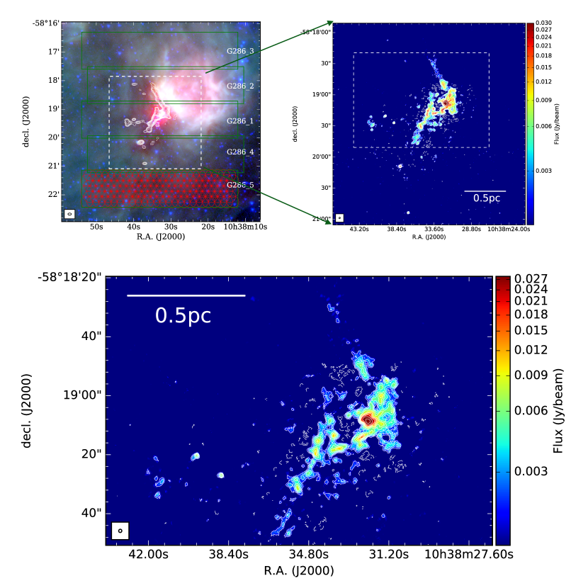
The observations were conducted with ALMA during Cycle 3 (Project ID 2015.1.00357.S, PI: J. C. Tan), during a period from Dec. 2015 to Sept. 2016. To map the entire field of G286 ($\sim$5.3′$\times$5.3′), we divided the region into five strips, denoted as G286_1, G286_2, G286_3, G286_4, and G286_5, each about $1\arcmin\>$ wide and $5.3\arcmin\>$ long and containing 147 pointings of the 12-m array. Figure 1a illustrates the spatial extent of the five strips, together with red circles showing the 12-m array mosaic footprints overlaid on strip G286_5 as an example. The position of field center is R.A.=10:38:33, decl.=-58:19:22. We employed the compact configuration C36-1 to recover scales between 1.5″ and 11.0″. Additionally, a 35-pointing mosaic was performed for each strip using the 7-m array, probing scales up to 18.6″. Total power observations of the region were also carried out (relevant only for the line observations).

Two scheduling blocks happened to be observed when the array configuration was in a transition phase, i.e., moving from a very extended configuration (C37/C38-1) to our proposed compact configuration. Thus we obtained extra $uv$ coverage for two strips, G286_1 and G286_2, where $\sim$90% of the continuum emission is located. This enables us to detect and characterize structures at a higher resolution ($\sim$1″, 2500 au) in these regions, which will be the focus of the results presented in this paper.

During the observations, we set the central frequency of the correlator sidebands to be the rest frequency of the $\rm{N_{2}D}^{+}$(3-2) line at $231.32\>$GHz for SPW0, and the $\rm{C^{18}O}$(2-1) line at $219.56\>$GHz for SPW2, with a velocity resolution of 0.046 and 0.048$\>\rm{km\>s}^{-1}$, respectively. The second baseband SPW1 was set to $231.00\>$GHz, i.e., 1.30 mm, to observe continuum with a total bandwidth of $2.0\>$GHz. The frequency coverage for SPW3 ranges from 215.85 to $217.54\>$GHz to observe DCN(3-2), DCO⁺(3-2), SiO($v=0$)(5-4) and $\rm{CH_{3}OH}(5_{1,4}-4_{2,2})$. The molecular line data from this observation will be presented and analyzed in a future paper, while here we focus on the results of the broad continuum band, i.e., tracing dust emission.

Both the 7-m and 12-m array data were calibrated with the data reduction pipeline using Casa 4.7.0. The continuum visibility data was constructed with all line-free channels. We performed imaging with tclean task in Casa and during cleaning we combined data for all five strips to generate a final mosaic map. The 7-m array data was imaged using a Briggs weighting scheme with a robust parameter of 0.5, which yields a resolution of $7.32\arcsec\times 4.42\arcsec\>$. For the combined data, we used the same Briggs parameter. In addition, since we have extra $uv$ coverage for part of the data, we also apply a 0.6″uvtaper to suppress longer baselines, which results in $1.62\arcsec\times 1.41\arcsec\>$ resolution.

The lowest noise level in the image varies from $0.2\>{\rm{mJy}}\>{\rm{beam}}^{-1}$ to $0.46\>{\rm{mJy}}\>{\rm{beam}}^{-1}$, depending on which strip is being considered. The $1\sigma$ noise of the central strip is $0.45\>{\rm{mJy}}\>{\rm{beam}}^{-1}$. We also do the cleaning separately for the central two strips with a smaller uvtaper value to utilize the long baseline data, which results in a resolution of 1.07″$\times$1.02″. The 1$\sigma$ noise level in this image is $0.45\>{\rm{mJy}}\>{\rm{beam}}^{-1}$.

Figure 1.— (a) Top Left: Three color image of G286 constructed by combining Spitzer IRAC 3.6 $\mu$m (blue), 8.0 $\mu$m (green), and Herschel PACS 70 $\mu$m (red). White contours show ALMA 7-m array image starting from 4$\sigma$. The G286 field is divided into five strips, as shown by the green rectangles. Each strip is covered with 147 pointings of the 12-m array, illustrated for strip G286_5 as an example with red circles marking the FWHM field of view of each pointing. The white dashed rectangle is the region shown in (b). (b) Top Right: Image with combined 12-m array and 7-m array data. The resolution is 1.62″$\times$1.41″. The contour levels are at (4, 8, 10, 12, 15, 20, 25, 30, 40, 50, 75, 100, 150)$\times 0.45\>{\rm mJy}\>{\rm beam}^{-1}$ (color scale in Jy beam^-1). The white dashed rectangle is the region shown in (c). (c) Bottom: Image with combined 12-m array and 7-m array data, but now imaged at 1.07″$\times$1.02″. Our CMF analysis is carried out for this region.

2.2. Core Identification

To study the CMF we first need to identify the “cores.” A variety of algorithms have been used to detect and characterise dense cores in previous studies of continuum maps (e.g., Williams et al. 1994; Kramer et al. 1998; Rosolowsky et al. 2008), and in practice, the results in terms of core number and statistical properties can vary with the different algorithms and input parameters (e.g., Pineda et al. 2009). To understand how the derived CMF depends on these identification methods, we thus adopt two well-documented and widely used algorithms to analyse our data and test the effects of variation of their parameters.

2.2.1 The Dendrogram Method

The dendrogram algorithm is described by Rosolowsky et al. (2008) and implemented in astrodendro. The dendrogram is an abstraction of the changing topology of the isosurfaces as a function of contour level. This method can describe hierarchical structures in a 2-D or 3-D datacube. There are two types of structures returned in the results: leaves, which have no sub-structure; and branches, which can split into multiple branches or leaves. Here we only use the leaf structure as a representation of dense cores.

There are three main parameters in this algorithm: $F_{\rm{min}}$, $\delta$, and $S_{\rm{min}}$. First, $F_{\rm{min}}$ is the minimum value to be considered in the dataset. In the fiducial case we adopt $F_{\rm{min}}=4\sigma$. Second, $\delta$ describes how significant a leaf has to be in order to be considered as an independent entity. We adopt a fiducial value of $\delta=1\sigma$, which means a core must have a peak flux reaching $5\sigma$ above the noise. The minimum area a structure must have to be considered as a core is given by $S_{\rm{min}}$. In general the size of the beam is a good choice, but in a crowded field a detected core can be smaller than one beam size due to blending, especially when a large value of $F_{\rm min}$ is used. We thus set $S_{\rm{min}}=0.5S_{\rm beam}$ as our fiducial choice. We will also explore the effects of varying these choices of $F_{\rm min}$, $\delta$, and $S_{\rm min}$.

2.2.2 The Clumpfind Method

The clumpfind algorithm (Williams et al. 1994) works by first contouring the data at a multiple of the rms noise of the observation, then searching for peaks of emission that locate the structure, then following them down to lower intensities. It was designed to study molecular clouds using 3-D datacubes and has also been widely used to describe dense cores (e.g., Reid & Wilson 2005; Pineda et al. 2009).

The most sensitive parameters for clumpfind are the lowest contour level ($F_{\rm min}$) and level spacing ($\Delta$). $F_{\rm min}$ is the same as that in the dendrogram method, and we adopt $4\sigma$ as a fiducial value. $\Delta$ refers to the contour level spacing and hence is somewhat different from the $\delta$ parameter of the dendrogram method. We choose $\Delta=3\sigma$ in the fiducial case, similar to previous implementations in the literature. As with the dendrogram method, cores are requires to have a minimum area $S_{\rm min}$, and we adopt $S_{\rm{min}}=0.5S_{\rm beam}$ as a fiducial threshold. Again, we investigate the effects of variations in the values of $F_{\rm min}$, $\Delta$, and $S_{\rm min}$.

Figure 2.— (a) Left: Cores found with the dendrogram method using our fiducial criteria: $F_{\rm min}=4\sigma$, $\delta=1\sigma$ and $S_{\rm min}=0.5S_{\rm beam}$. The image is shown in gray scale overlaid on black contours starting from 4$\sigma$ and increasing in steps of 2$\sigma$. The red contours indicate the boundaries of the detected cores. (b) Right: Same as (a), but now showing the results of the clumpfind method. The criteria are $F_{\rm min}=4\sigma$, $\Delta=1\sigma$ and $S_{\rm min}=0.5S_{\rm beam}$.

2.3. Core Mass Estimation

We estimate core masses by assuming optically thin thermal emission from dust. The total mass surface density corresponding to a given specific intensity of mm continuum emission is

$$\Sigma_{\rm mm} = 0.369\frac{F_{\nu}}{\rm mJy}\frac{(1\arcsec)^{2}}{\Omega}\frac{\lambda_{1.3}^{3}}{\kappa_{\nu,0.00638}}$$

$$\times\left[{\rm exp}\left(0.553T_{d,20}^{-1}\lambda_{1.3}^{-1}\right)-1\right]\>{\rm g\>cm^{-2}}$$

$$\rightarrow 0.272\frac{F_{\nu}}{\rm mJy}\frac{(1\arcsec)^{2}}{\Omega}\>{\rm g\>cm^{-2}},$$

where $F_{\nu}$ is the total integrated flux over solid angle $\Omega$, $\kappa_{\nu,0.00638}\equiv\kappa_{\nu}/({\rm 6.38\times 10^{-3}\>cm^{2}\>g}^{-1})$ is the dust absorption coefficient, $\lambda_{1.3}=\lambda/1.30\>{\rm mm}$ and $T_{d,20}=T_{d}/20\>{\rm K}$ with $T_{d}$ being the dust temperature. To obtain the above fiducial normalization of $\kappa_{\nu}$, we assumed an opacity per unit dust mass $\kappa_{\rm 1.3mm,d}=0.899\>{\rm cm^{2}g}^{-1}$ (moderately coagulated thin ice mantle model of Ossenkopf & Henning 1994), which then gives $\kappa_{\rm 1.3mm}={\rm 6.38\times 10^{-3}\>cm^{2}\>g}^{-1}$ using a gas-to-refractory-component-dust ratio of 141 (Draine 2011). The numerical factor following the $\rightarrow$ in the final line shows the fiducial case where $\lambda_{1.3}=1$ and $T_{d,20}=1$.

Note that since we do not have detailed temperature information for each source, for simplicity we have adopted an uniform value of $T_{d}=20\>$ K for all cores in our fiducial analysis. Such temperatures are expected to be representative of average temperatures in protostellar cores (e.g., Zhang & Tan 2015). However, we recognize that somewhat warmer temperatures may result either from strong external heating by nearby, luminous sources in the embedded protocluster or by stronger than average internal heating in protostellar cores. On the other hand, the temperature could be lower in prestellar or early-stage protostellar cores. If temperatures of 15 K or 30 K were to be adopted, then the mass estimates would differ by factors of 1.48 and 0.604, respectively.

Given the above values of $\Sigma_{\rm mm}$, then the core mass is

$$M = \Sigma_{\rm mm}A=0.113\frac{\Sigma_{\rm mm}}{\rm g\>cm^{-2}}\frac{\Omega}{(1\arcsec)^{2}}\left(\frac{d}{\rm 1\>kpc}\right)^{2}\>M_{\odot}$$

$$\rightarrow 0.192\frac{F_{\nu}}{\rm mJy}\left(\frac{d}{\rm 2.5\>kpc}\right)^{2}\>M_{\odot}$$

where $A$ is the projected area of the core, $d$ is the source distance, and the final evaluation is for fiducial temperature assumptions of 20 K (following eq. 2.3). Thus the $1\sigma$ noise level in the image corresponds to a core mass of $\sim 0.1\>M_{\odot}$.

Overall, we estimate absolute mass uncertainties of about a factor of two, which we expect to be caused mostly by temperature variations. Relative core mass estimates will be somewhat more accurate, although still potentially with uncertainties of this magnitude due to core to core temperature and opacity variations.

2.4. Core Flux Recovery and Completeness Corrections

We calculate two corrections factors that are needed to estimate a “true” CMF from a “raw” observed CMF. First, since both dendrogram and clumpfind methods adopt a threshold value (i.e., 4$\sigma$) and pixels below this level are not assigned to any core structures, we expect the estimated core flux (i.e., mass) is a fraction of the true flux. We estimate the flux recovery fraction, $f_{\rm flux}$, as a function of true core mass by carrying out experiments of artificial core insertion into the ALMA images. These same experiments also allow us to assess the second factor, i.e., the number recovery fraction, $f_{\rm num}$, again as a function of true input core mass. These correction factors are also expected to depend on core density profile and the local clump environment, e.g., degree of crowding.

We adopt the following methods for these experiments of artificial core insertion and recovery. The artificial cores are assumed to have the same shape as the synthesized beam, i.e., the limiting case appropriate for small, unresolved cores. The locations of the artificial cores are chosen randomly, but with a probability density that is scaled to match the flux profile we derive from the 7-m array image, which has the effect of placing more cores in crowded regions. In each experiment, we insert 10 cores (i.e., $\sim$10% of the total number to avoid excessive blending) of a given total flux, i.e., of a given mass. We run the core detection algorithms to determine the average flux levels recovered in detected cores and the probability for artificial cores of a given mass to be found. This is repeated 30 times to obtain a large sample for more accurate estimates.

With $f_{\rm flux}(M)$ estimated in this way, we then first transform the raw CMF into a flux-corrected CMF, which involves estimating the average (median) flux correction factor for a given observed mass. Then, given our estimate of $f_{\rm num}(M)$, we transform the flux-corrected CMF into an estimate of the true CMF, i.e., by assuming the completeness correction factor at a given mass is equal to the inverse of $f_{\rm num}$. The derived forms of $f_{\rm flux}(M)$ and $f_{\rm num}(M)$ are shown in the next section for our fiducial case.

3. Results

3.1. 1.3 mm Continuum Image

Figure 1 presents the $1.3\>$mm continuum map constructed with the 7-m array data in the top left panel, 12-m and 7-m array combined data in the top right panel, and the highest resolution combined image in the bottom panel. The image with only 7-m data reveals two main filaments: a northern one with a NE–SW orientation and a southern one with a NW–SE orientation. These two filaments converge at a clump with bright mm continuum emission. Several other isolated clumps are also revealed. The southern filament and central hub are further resolved into a cluster of dense cores. The image combining all data has a spatial dynamic range that recovers structures from $\sim 1\arcsec$ to $\sim 20\arcsec$.

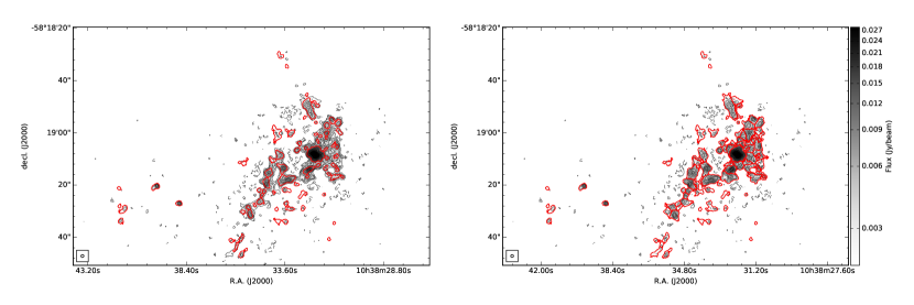
Figure 2 shows the high resolution ($\sim 1\arcsec$) 1.3 mm continuum image with the core boundaries overlaid for both the dendrogram and clumpfind methods. Inspection of these images allows one to assess how the core identification algorithms operate on the imaging data. One sees cores with a range of sizes, some being many times the size of the beam. Note that the central, brightest and most massive “core” is identified in a similar way with both algorithms. However, we expect that there is a high probability that such massive, large area “cores” will appear fragmented when imaged at higher angular resolution (see also §4).

Another feature revealed by Figure 2 is clumpfind’s method of partitioning all the flux above the minimum threshold contour level. This is to be contrasted with the method adopted by the dendrogram algorithm, with the effect being to tend to make the cores identified by clumpfind more massive than their dendrogram counterparts.

3.2. The Core Population and CMF

Figure 3.— (a) Top: CMF for the dendrogram method. The original CMF is shown in black and after mass (flux) correction for each core is shown in blue. The blue CMF is then corrected for the number recovery fraction, as illustrated in red. The dashed lines in black, blue and red show the best power law fit result for the high-mass end ($M>0.8\>M_{\odot}$) for the corresponding CMFs. (b) Bottom: As (a), but now for the clumpfind method.

Figure 4.— (a) Top: Flux recovery fraction, $f_{\rm flux}$, versus core mass, $M$, for dendrogram and clumpfind algorithms, as labelled. (b) Bottom: Number recovery fraction, $f_{\rm num}$, versus core mass, $M$, for dendrogram and clumpfind algorithms, as labelled.

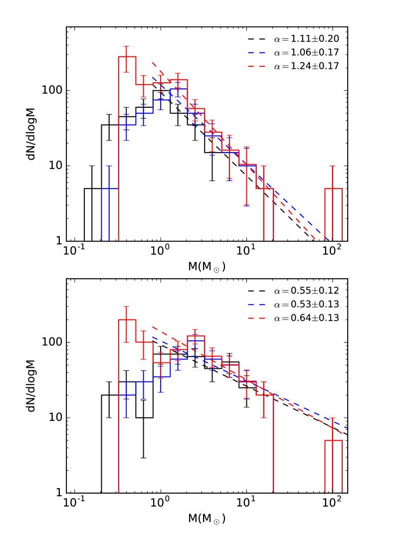
In Figure 3 we show the “raw” CMFs (black histograms) derived from our fiducial dendrogram (top panel) and clumpfind (bottom panel) methods. The fiducial dendrogram method ($F_{\rm min}=4\sigma$, $\delta=1\sigma$, $S_{\rm min}=0.5S_{\rm beam}$) identifies 76 cores, while the fiducial clumpfind method ($F_{\rm min}=4\sigma$, $\Delta=3\sigma$, $S_{\rm min}=0.5S_{\rm beam}$) finds 83 cores. Note, we adopt uniform binning in ${\rm log}\>M$, with 5 bins per dex. Poisson counting errors are shown for each bin. Figure 3 also displays the flux corrected CMFs (blue histograms, with errors again estimated as a Poisson value) and subsequently number corrected, i.e., “true,” CMFs (red histograms, with error assumed to be the same fractional value as in the blue histograms), for each case. The fitting of power law functions to the high-mass end of the CMFs is discussed below.

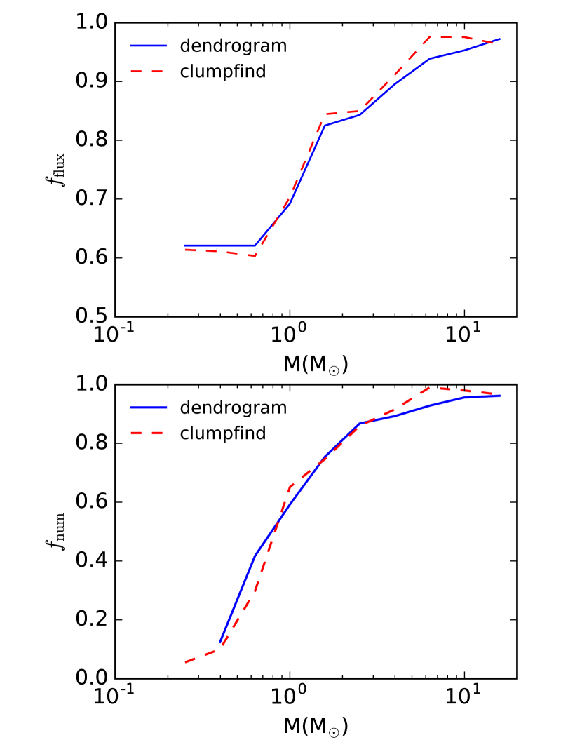
The correction factors used in Figure 3 are shown in Figure 4. The flux correction factor, which is based on median values of $f_{\rm flux}$ (excluding values $>1$, which we attribute to false assignments; and extrapolating with constant values for $M\lesssim 0.3\>M_{\odot}$), rises from about 0.6 at the low-mass end (when cores are detected) to close to unity at the high-mass end. The values of $f_{\rm flux}$ for dendrogram and clumpfind are similar to each other, with clumpfind recovering slightly more flux over most of the mass range.

The number recovery fractions, $f_{\rm num}$, show a larger dynamic range, rising from $\sim 0.1$ at the low-mass end to near unity at the high-mass end (these remain slightly less than one due to the possibility of blending with existing massive cores). Again, the values of this correction factor are similar for both dendrogram and clumpfind. We estimate that we are about 50% complete by number for $\sim 1\>M_{\odot}$ cores. The direct effect of the number correction can be seen by comparing the blue and red histograms in Fig. 3.

We characterize the high-end ($>0.8\>M_{\odot}$, i.e., starting with the bin centered on $1\>M_{\odot}$) part of the raw dendrogram CMF by fitting a power law of the form given by equation (1). We find $\alpha=1.11\pm 0.20$. Fitting the same mass range for the flux corrected CMF yields $\alpha=1.06\pm 0.17$, while that for the fully (flux and number) corrected, i.e., “true”, CMF yields $\alpha=1.24\pm 0.17$. Thus these correction factors have only a modest impact on the shape of the CMF for $M\gtrsim 0.8\>M_{\odot}$, with the true CMF being slightly steeper than the raw CMF, mostly due the effects of the number correction.

We note that there is sparse sampling of the high-mass end of the CMF, i.e., there is a single, massive ($\sim 100\>M_{\odot}$) “core.” Our fitting method, which we note minimizes $\chi^{2}$ in log space, treats the empty bins as effective upper limits. However, if we were to exclude this source and fit the CMF only over the range from 0.8 to $\sim 20\>M_{\odot}$, then we would derive $\alpha=1.11\pm 0.22$ and $\alpha=1.15\pm 0.17$ for the raw and true CMFs, respectively, i.e., there is only a very minor effect.

Inspection of the true CMF indicates that the power law behavior may continue down to lower masses. If we fit to the range $M\gtrsim 0.3\>M_{\odot}$, we derive a moderately shallower value of $\alpha=0.83\pm 0.11$. From these results, we see that there is potential evidence for a break in the CMF near $1\>M_{\odot}$, but that a single power law is still a reasonable description of the flux and number corrected, i.e., true, CMF across most of the mass range probed, i.e., from $\sim 0.3\>M_{\odot}$ to $\sim 100\>M_{\odot}$.

For the CMF resulting from the fiducial clumpfind algorithm, the power law description of the raw CMF also appears potentially valid for $M\gtrsim 0.8\>M_{\odot}$. For this we derive $\alpha=0.55\pm 0.12$, which is significantly shallower than the $1.11\pm 0.20$ derived over the same mass range for the dendrogram raw CMF. Thus, note, there are a larger number of massive cores found with the clumpfind method than with the dendrogram method. Then, on applying the flux and number corrections, the “true” CMF found via clumpfind displays a local peak at about $2.5\>M_{\odot}$, but with numbers of lowest-mass cores still potentially rising slowly. If we attempt the same uniform metric of a single power law fit above $0.8\>M_{\odot}$, then we find $\alpha=0.64\pm 0.13$. If we fit only from the bin containing the true CMF peak and extending to higher masses, then we find $\alpha=0.78\pm 0.14$, which is still shallower than the equivalent dendrogram result.

Thus we see that whether or not there is a peak or break defining a characteristic mass in the CMF depends on the method of core identification used and whether or not completeness corrections are applied. In particular, while the two methods find similar number of cores, we can explain the differences in their final CMFs mostly as a result of how mass is then assigned to the identified structures. As discussed above, clumpfind partitions all the flux above a given threshold to the sources, while dendrogram does not, i.e., its cores sit on plateaux that are described by branches in its structural decomposition.

Figure 5.— Raw CMFs derived with results from the dendrogram method shown on the top panels, and the clumpfind method on the bottom panels. For each algorithm we show different results by varying $F_{\rm min}$, $\delta$ (for dendrogram and $\Delta$ for clumpfind) and $S_{\rm min}$ (columns, left to right). In each panel, the results with different parameter selections are illustrated in different colors (see text). The number in the brackets denotes how many cores are detected. Also shown is the power law index, $\alpha$, from fitting the high-mass end ($M>0.8\>M_{\odot}$ for both dendrogram and clumpfind).

The values of high-end slopes of the CMFs are relatively unaffected by the application of the completeness corrections. We note that the stellar IMF at $\gtrsim 1\>M_{\odot}$ also follows a power law form with $\alpha\simeq 1.35$ (Salpeter 1955), and this value is very similar to those seen in the dendrogram CMFs, while the clumpfind CMFs are shallower. As previous studies of more local regions have found (see §1), this may indicate that core to star formation efficiency is relatively constant with increasing mass, at least over the range of masses that is effectively probed here, i.e., from $\sim 1$ to $\sim 100\>M_{\odot}$. The outflow and radiative feedback models of Tanaka et al. (2017) for star formation in clumps with $\Sigma_{\rm cl}\simeq 1\>{\rm g\>cm}^{-2}$, i.e., the value most relevant to G286, predict that these efficiencies should drop from $\epsilon=$0.48 to 0.37 as the stellar mass increases from $5\>M_{\odot}$ to $40\>M_{\odot}$, i.e., as core masses increase from about $10\>M_{\odot}$ to about $100\>M_{\odot}$. Such a relatively small change in $\epsilon$ is still compatible with the results we have presented, since they lack significant numbers of cores $>20\>M_{\odot}$ to place very stringent constraints in this regime. Other caveats should also be considered that may affect the derived CMFs, including possible systematic temperature variations with increasing continuum flux, i.e., if brighter cores are warmer, we will have overestimated their masses. However, with the data in hand, it is not currently possible to assess how important this effect may be.

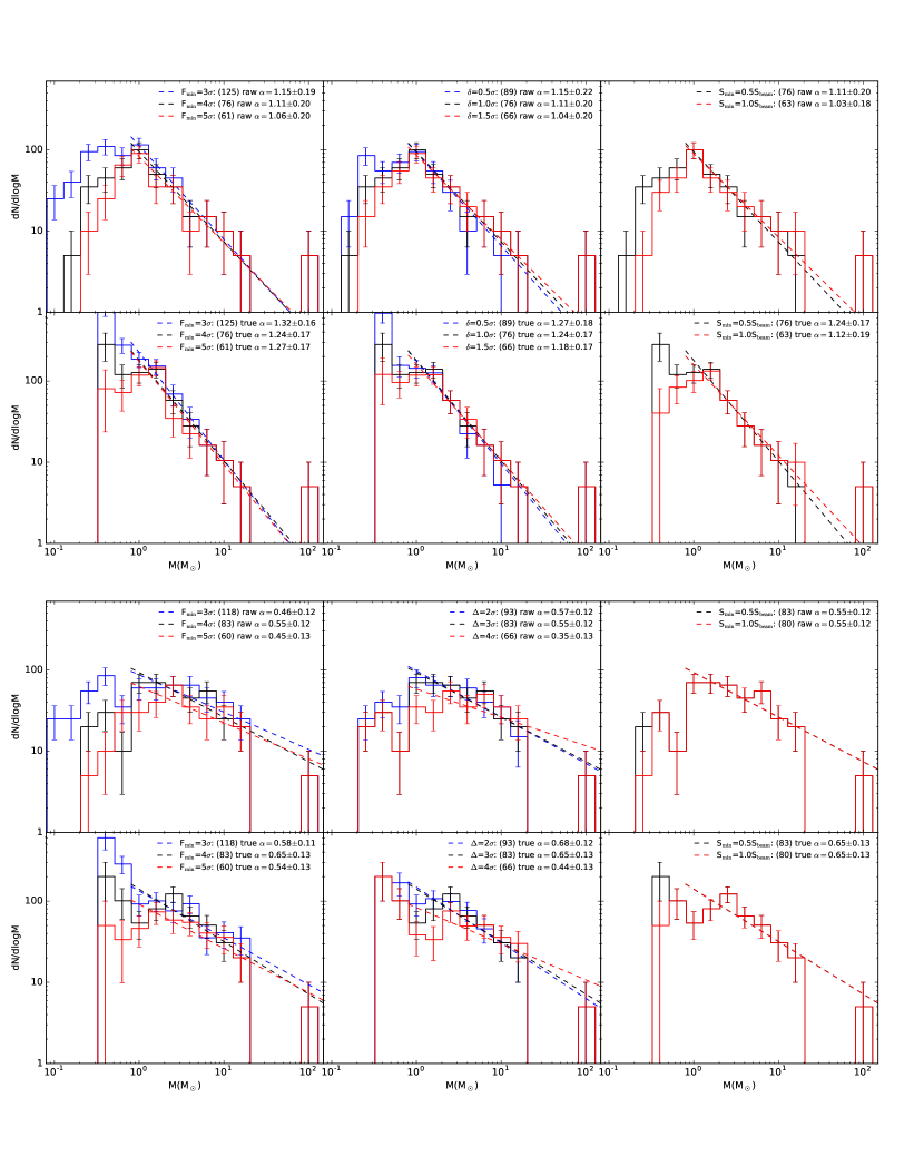
In Figure 5 we show the dependence of the CMFs that result from varying the three main parameters associated with each core identification method. We focus on the total core numbers found, the shape of the raw and true CMFs, and the high-end slope of the power law fits. In relation to the fiducial dendrogram method, if we lower the minimum threshold to $F_{\rm min}=3\sigma$, 125 cores are now found (total core numbers are listed in parentheses in the legend in Fig. 5), with the increase mostly being for sub-solar mass cores. If we set $F_{\rm min}=5\sigma$, then only 61 cores are recovered. Varying $\delta$ to $0.5\sigma$ or $1.5\sigma$ has a more modest effect, as does increasing the minimum size of a core to 1 beam area. We see from comparing the raw CMFs and their derived values of $\alpha$ that the shape above $1\>M_{\odot}$ is relatively robust to these variations. In fact, we note that all the variation we see in $\alpha$ of these raw CMFs due to different dendrogram parameter choices is smaller than the uncertainty arising from Poisson counting statistics in this fiducial estimate. The completeness-corrected “true” CMFs found by the different dendrogram methods are generally very similar to one another if one restricts attention to $M\gtrsim 1\>M_{\odot}$, where the power law fits are always found to be slightly steeper than those of the raw CMFs. However, the shapes of these true CMFs below $1\>M_{\odot}$ are quite strongly affected by the choice of core definition within the dendrogram framework. This can affect whether or not a characteristic core mass is seen in the CMFs.

We have seen that the fiducial clumpfind method yields similar core numbers as the dendrogram analysis. Figure 5 shows that this is also true if we consider variations in its parameters $F_{\rm min}$ and $\Delta$, in correspondence with the variations of the equivalent dendrogram parameters. However, unlike dendrogram, clumpfind does not see a significant reduction in the numbers of cores found if the minimum core size is doubled. Again, most values of the high-end $\alpha$ of these raw and true CMFs are similar to the fiducial values of their respective cases, i.e., 0.55 and 0.65, with only the $\Delta=4\sigma$ case yielding significantly shallower slopes.

Figure 6.— CMFs derived for images with lower spatial resolution, i.e., “1.5″” (actually 1.62″$\times$1.41″), shown as red histograms and fitted power laws. These are compared to the fiducial results from analysis of the “1″” images (actually $1.07\arcsec\times 1.02\arcsec$), shown in black. Top left: Raw CMFs with the fiducial dendrogram method. Bottom left: Completeness-corrected true CMFs with the fiducial dendrogram method. Top right: Raw CMFs with the fiducial clumpfind method. Bottom right: Completeness-corrected true CMFs with the fiducial clumpfind method.

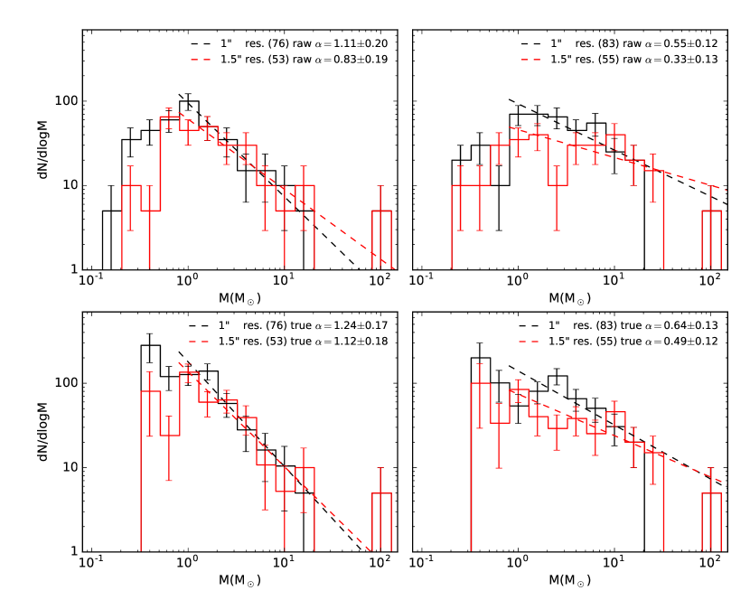
Next, we examine how the CMFs vary if the analyzed image has a lower angular resolution of $\simeq 1.5\arcsec$. Figure 6 compares the raw CMFs derived from the $1\arcsec$ and $\simeq 1.5\arcsec$ images. As expected, core masses tend to shift to higher values when identified from the lower resolution image. This leads to a flattening in the shape of the high-end CMFs, i.e., a reduction in the derived values of $\alpha$, which can be quite significant, i.e., $\Delta\alpha\simeq-0.3$ for the raw CMF found by the fiducial dendrogram method. However, after completeness corrections are applied, the effect on $\alpha$ is more modest. These results indicate that even the high-end part of the CMFs can vary somewhat as the resolution is changed, and the trend may continue in the opposite direction if one were to image at higher resolutions. Indeed, this is expected if the more massive, larger cores are seen to fragment at significant levels when imaged at higher resolution. Such cores are known to fragment to some extent, although there are observed cases of quite limited fragmentation (e.g., Csengeri et al. 2017). This effect should be kept in mind when comparing CMFs derived from protoclusters that are observed with different resolutions, e.g., as may occur due to being at different distances.

Figure 7.— CMFs derived for images derived from only the 12m-array data, shown as red histograms and fitted power laws. These are compared to the fiducial results from analysis of our 12m + 7m array combined images, shown in black. Top left: Raw CMFs with the fiducial dendrogram method. Bottom left: Completeness-corrected true CMFs with the fiducial dendrogram method. Top right: Raw CMFs with the fiducial clumpfind method. Bottom right: Completeness-corrected true CMFs with the fiducial clumpfind method.

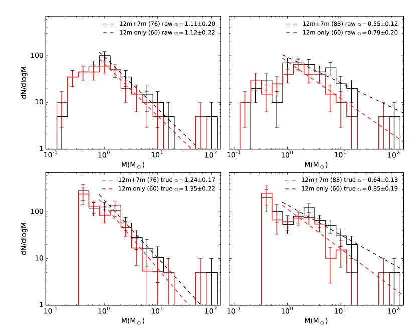
Finally, in Figure 7 we examine how the CMFs vary if the analyzed image is lacking the larger spatial scales obtained from the 7m-array data. Such an analysis is useful for understanding how the results of other observational programs that measure CMFs without such data may be affected. Our 12m only image has an rms noise level of 0.47 mJy beam^-1. For the dendrogram method we find that the CMF derived from the 12m only image contains slightly fewer cores (60) than found in the combined image (76), but has a high-end power law slope index that is very similar. For the completeness-corrected CMF the 12m-array only CMF has a high-end power law index that is about 0.1 steeper than that derived from the 12m + 7m image. Similar results are also found for clumpfind derived raw and true CMFs, with the difference now being about 0.2 in the magnitude of $\alpha$. Thus the value of the high-end power law slope of the true CMF appears to be slightly over estimated if the image is lacking the larger spatial scales provided by 7m-array data.

4. Discussion and Conclusions

We have studied the CMF in the central region of the massive protocluster G286.21+0.17, with cores identified by their 1.3 mm dust continuum emission in a high spatial dynamic range image observed with the 7-m and 12-m arrays of ALMA. We explored the effects of using two different core identification algorithms, dendrogram and clumpfind, including a systematic study of the effects of varying their three main core selection parameters. We also examined the effects of varying angular resolution and largest recovered angular scale of the analyzed continuum image.

Our fiducial methods, including flux and number corrections estimated by artificial core insertion and recovery, yield CMFs that show high-end ($M\gtrsim 1\>M_{\odot}$) power law indices of $\alpha=1.24\pm 0.17$ for dendrogram and $0.64\pm 0.13$ for clumpfind. These results are quite robust to variations of choices of core selection parameters.

With the dendrogram method, which we consider to be preferable to clumpfind as a means for identifying and characterizing cores that are embedded in a clump environment, these power law indices are similar to the Salpeter stellar IMF index of 1.35. This further strengthens the case of a correspondence between CMF and IMF seen in local regions, but now in a more distant, massive protocluster. As discussed in §1, such a correspondence is a general feature and/or expectation of Core Accretion models of star formation, in contrast to Competitive Accretion models. However, caveats remain, including potential systematic changes in core temperature for brighter cores and the fact that the measured CMF is expected to be composed of a mixture of prestellar and protostellar cores, i.e., tracing different evolutionary stages (see also discussion of Clark et al. 2007).

We do find that whether or not a peak is seen in the CMF near $1\>M_{\odot}$ depends on which core finding algorithm is used, i.e., dendrogram or clumpfind, the choices of parameters associated with the algorithm, and whether or not completeness corrections are carried out. Thus we cannot make firm conclusions about the presence of a peak or characteristic core mass near $1\>M_{\odot}$. Such a peak might be expected if there is close correspondence of CMF shape with stellar IMF shape. Our fiducial dendrogram result (see Fig. 3a) shows only a very tentative hint of there being a break in the power law description of the CMF to shallower slopes for masses $\lesssim 1\>M_{\odot}$.

We re-emphasize that the relation of the CMF identified purely from sub-mm/mm dust continuum emission to the stellar IMF is uncertain. We expect that many of the cores identified by these methods, being the brighter cores, will be protostellar sources. Examples of massive prestellar cores identified by their high levels of deuteration, i.e., via $\rm N_{2}D^{+}$ line emission, can show relatively weak mm continuum emission, perhaps indicating that they are significantly colder than their surrounding clump material (Kong et al. 2017a,b). For constraining theoretical models, it is desirable to have a measure of the PSCMF, and it remains to be seen how effective interferometric studies of mm continuum emission in distant massive protoclusters are at measuring this PSCMF (see, e.g., Fontani et al. 2009).

The observations carried out here also included $\rm N_{2}D^{+}$(3-2) and ¹²CO(2-1), amongst other species. In a future paper, these line data will be analyzed to place better constraints on the PSCMF and its relation to the CMFs presented here. We note that core finding methods that also utilize molecular line emission may also make it easier to break-up spatially confused structures.

Another caveat in the accuracy of CMF determination relates to the effects of spatial resolution and the possibility of fragmentation of identified “cores” into smaller structures as the resolution is increased. Such an effect has been seen before in numerous studies, but at varying levels (e.g., Beuther & Schilke 2004; Bontemps et al. 2010; Zhang et al. 2015; Csengeri et al. 2017). Cases of limited fragmentation may indicate an important role for magnetic fields in stabilizing the more massive cores (see, e.g., Kunz & Mouschovias 2009; Tan et al. 2013; Fontani et al. 2016). Our investigation of how the true dendrogram CMF varies as the resolution is changed from about 1.5″ to 1″ shows that there is a slight steepening of the power law index, by about 0.1, as one goes to the higher resolution. However, the size of this change is smaller than the uncertainties arising solely from counting statistics, so larger samples of cores are needed to verify this trend. Higher sensitivity and higher angular resolution studies of the G286.21+0.17 are also desirable to investigate the particular fragmentation properties of the identified cores.

Taking the above caveats of CMF definition in mind, we still regard characterization of the mm continuum image via identification of discrete cores by specified, well-defined algorithms as a useful exercise for assessing the fragmentation in the cloud and as a first step for measuring the true CMF and, eventually, the PSCMF. Furthermore, the same core finding algorithms can also be applied to simulated molecular clouds to make a direct, statistical comparison of their structures with those of real systems, and in this way constrain the physics of star and star cluster formation.

References

- Alves et al. (2007) Alves, J., Lombardi, M., & Lada, C. J. 2007, A&A, 462, L17
- Andersen et al. (2017) Andersen, M., Barnes, P., Tan, J. C., Kainulainen, J. & de Marchi, G. 2017, AJ, accepted (arXiv:1709.10448)
- André et al. (2010) André, P., Men’shchikov, A., Bontemps, S., et al. 2010, A&A, 518, L102
- André et al. (2014) André, P., Di Francesco, J., Ward-Thompson, D., et al. 2014, Protostars and Planets VI, 27
- Barnes et al. (2010) Barnes, P. J., Yonekura, Y., Ryder, S. D., et al. 2010, MNRAS, 402, 73
- Barnes et al. (2011) Barnes, P. J., Yonekura, Y., Fukui, Y. et al. 2011, ApJS, 196, 12
- Bastian et al. (2010) Bastian, N., Covey, K. R., & Meyer, M. R. 2010, ARA&A, 48, 339
- Bate (2012) Bate M. R. 2012, MNRAS, 419, 3115
- Beuther et al. (2006) Beuther, H., Zhang, Q., Sridharan, T. K., Lee, C.-F., & Zapata, L. A. 2006, A&A, 454, 221
- Bonnell et al. (2001) Bonnell I. A. et al. 2001, MNRAS, 323, 785.
- Bontemps et al. (2010) Bontemps, S., Motte, F., Csengeri, T., & Schneider, N. 2010, A&A, 524, A18
- Chira et al. (2013) Chira, R.-A. et al. 2013, A&A, 552, 40
- Clark et al. (2007) Clark, P. C., Klessen, R. S. & Bonnell, I. A. 2007, MNRAS, 379, 57
- Csengeri et al. (2017) Csengeri, T., Bontemps, S., Wyrowski, F. et al. 2017, A&A, 600, L10
- Draine (2011) Draine B. T. 2011, Physics of the Interstellar and Intergalactic Medium (Princeton: Princeton Univ. Press)
- Fontani et al. (2016) Fontani, F., Commerçon, B., Giannetti, A. et al. 2016, A&A, 593, L14
- Fontani et al. (2009) Fontani, F., Zhang, Q., Caselli, P., & Bourke, T. L. 2009, A&A, 499, 233
- Hennebelle & Chabrier (2008) Hennebelle, P. & Chabrier, G. 2008, ApJ, 684, 395
- Johnstone et al. (2000) Johnstone, D., Wilson, C. D., Moriarty-Schieven, G., et al. 2000, ApJ, 545, 327
- Kong et al. (2017a) Kong, S., Tan, J. C., Caselli, P. et al. 2017a, ApJ, 834, 1
- Kong et al. (2017b) Kong, S., Tan, J. C., Caselli, P. et al. 2017b, ApJ, submitted (arXiv:1701.05953)
- Kramer et al. (1998) Kramer, C., Stutzki, J., Rohrig, R. & Corneliussen, U. 1998, A&A, 329, 249
- Kroupa et al. (2013) Kroupa, P., Weidner, C., Pflamm-Altenburg, J., et al. 2013, Planets, Stars and Stellar Systems. Volume 5: Galactic Structure and Stellar Populations, 5, 115
- Kunz & Mouschovias (2009) Kunz, M. W. & Mouschovias, T. Ch. 2009, MNRAS, 399, L94
- Ma et al. (2013) Ma, B., Tan, J. C. & Barnes, P. J. 2013, ApJ, 779, 79
- Marsh et al. (2016) Marsh, K. A., Kirk, J. M., André, P., et al. 2016, MNRAS, 459, 342
- Matzner & McKee (2000) Matzner, C. D., & McKee, C. F. 2000, ApJ, 545, 364
- McKee & Tan (2003) McKee, C. F., & Tan, J. C. 2003, ApJ, 585, 850
- Motte et al. (1998) Motte, F., Andre, P., & Neri, R. 1998, A&A, 336, 150
- Nutter & Ward-Thompson (2007) Nutter, D., & Ward-Thompson, D. 2007, MNRAS, 374, 1413
- Ohashi et al. (2016) Ohashi, S., Sanhueza, P., Chen, H.-R. V., et al. 2016, ApJ, 833, 209
- Ossenkopf & Henning (1994) Ossenkopf V. & Henning T. 1994, A&A, 291, 943
- Padoan & Nordlund (2002) Padoan, P., & Nordlund, A. 2002, ApJ, 576, 870
- Padoan & Nordlund (2007) Padoan, P., & Nordlund, A. 2007, ApJ, 661, 972
- Pillai et al. (2006) Pillai, T., Wyrowski, F., Carey, S. J., & Menten, K. M. 2006, A&A, 450, 569
- Pineda et al. (2009) Pineda, J. E., Rosolowsky, E. W., & Goodman, A. A. 2009, ApJ, 699, L134
- Reid & Wilson (2005) Reid, M. A. & Wilson, C. D. 2005, ApJ, 625, 891
- Rodón et al. (2012) Rodón, J. A., Beuther, H., & Schilke, P. 2012, A&A, 545, A51
- Rosolowsky et al. (2008) Rosolowsky, E. W., Pineda, J. E., Kauffmann, J. & Goodman, A. A. 2008, ApJ, 679, 1338
- Sadavoy et al. (2010) Sadavoy, S. I., Di Francesco, J., Bontemps, S., et al. 2010, ApJ, 710, 1247
- Salji et al. (2015) Salji, C. J., Richer, J. S., Buckle, J. V., et al. 2015, MNRAS, 449, 1782
- Salpeter (1955) Salpeter, E. E. 1955, ApJ, 121, 161
- Tan et a. (2013) Tan, J. C., Kong, S., Butler, M. J. et al. 2013, ApJ, 779, 96
- Tanaka et al. (2017) Tanaka, K. E. I., Tan, J. C., & Zhang, Y. 2017, ApJ, 835, 1
- Testi & Sargent (1998) Testi, L., & Sargent, A. I. 1998, ApJ, 508, L91
- Wang et al. (2008) Wang Y., Zhang Q., Pillai, T. et al. 2008, ApJ, 672, L33
- Williams et al. (1994) Williams, J. P., de Geus, E. J., & Blitz, L. 1994, ApJ, 428, 693
- Zhang et al. (2015) Zhang, Q., Wang, K., Lu, X., & Jiménez-Serra, I. 2015, ApJ, 804, 141
- Zhang et al. (2014) Zhang, Y., Tan, J. C. & Hosokawa, T. 2014, ApJ, 788, 166