Early propagation of energetic particles across the mean field in turbulent plasmas

Abstract

Propagation of energetic particles across the mean field direction in turbulent magnetic fields is often described as spatial diffusion. Recently, it has been suggested that initially the particles propagate systematically along meandering field lines, and only later reach the time-asymptotic diffusive cross-field propagation. In this paper, we analyse cross-field propagation of 1–100 MeV protons in composite 2D-slab turbulence superposed on a constant background magnetic field, using full-orbit particle simulations, to study the non-diffusive phase of particle propagation with a wide range of turbulence parameters. We show that the early-time non-diffusive propagation of the particles is consistent with particle propagation along turbulently meandering field lines. This results in a wide cross-field extent of the particles already at the initial arrival of particles to a given distance along the mean field direction, unlike when using spatial diffusion particle transport models. The cross-field extent of the particle distribution remains constant for up to tens of hours in turbulence environment consistent with the inner heliosphere during solar energetic particle events. Subsequently, the particles escape from their initial meandering field lines, and the particle propagation across the mean field reaches time-asymptotic diffusion. Our analysis shows that in order to understand solar energetic particle event origins, particle transport modelling must include non-diffusive particle propagation along meandering field lines.

1 Introduction

Understanding the propagation of energetic particles in turbulent plasmas is the key for understanding the acceleration of solar energetic particles (SEPs), and their relation to the complex phenomena during solar eruptions. The propagation of these charged particles is affected by the heliospheric electric and magnetic fields. The particles are guided by the Parker spiral field, and experience guiding centre drifts across the field (e.g. Marsh et al., 2013). The turbulent fluctuations in the magnetic field, on the other hand, bring a stochastic element to the propagation of the particles, often modelled as diffusion along and across the mean field direction (Parker, 1965).

Energetic particle propagation across the mean magnetic field in turbulent plasmas has been considered as mainly the effect of particles following the meandering field lines (e.g. Jokipii, 1966). Current approaches aiming to quantify this effect take into account scattering of the particles along the field lines (Matthaeus et al., 2003; Shalchi, 2010). Also the decoupling of the particles from the field lines has been considered (Fraschetti & Jokipii, 2011; Ruffolo et al., 2012). These theoretical approaches work towards a time-asymptotic description of particle cross-field transport as a spatial diffusion process. Cross-field diffusion description has recently been applied also in modelling the SEP propagation in the heliosphere (Zhang, Qin & Rassoul, 2009; Dröge et al., 2010; He, Qin & Zhang, 2011; Tautz, Shalchi & Dosch, 2011; Giacalone & Jokipii, 2012; Qin et al., 2013; Strauss, Dresing & Engelbrecht, 2017).

However, Laitinen, Dalla & Marsh (2013) noted recently that early in the propagation history, particles propagate systematically along meandering field lines, spreading efficiently across the mean field direction (see also Tooprakai et al., 2016). This spreading is non-diffusive in nature, and only at later times the particles decouple sufficiently from their meandering field lines, resulting in propagation that can be described as diffusion across the mean magnetic field. Using full-orbit particle simulations in a cartesian geometry, Laitinen, Dalla & Marsh (2013) concluded that the temporal and spatial evolution of impulsively-injected 10 MeV protons, as recorded 1 AU from the injection region, remained inconsistent with diffusion description for $\sim 20$ hours after the particle injection. Thus, the non-diffusive early propagation may be very significant to the propagation of the SEPs from the Sun to the Earth. Laitinen et al. (2016) showed that the wide SEP events observed with multiple spacecraft at different heliographic longitudes at 1 AU (e.g. Lario et al., 2013; Dresing et al., 2012; Wiedenbeck et al., 2013; Dresing et al., 2014; Cohen et al., 2014; Richardson et al., 2014) could be explained using this approach with particle transport parameters consistent with the interplanetary turbulence properties already with a narrow source at the Sun.

The initial study by Laitinen, Dalla & Marsh (2013) only addressed one set of particle and turbulence parameters, and did not explore the parameter space of particle and turbulence further to identify properties that may influence the initial non-diffusive particle propagation phase. In this work, we will study the initial non-diffusive phase and the asymptotic diffusive phase in more detail, varying both the particle and turbulence parameters. We will study the nature of the transition from the initial to the asymptotic phase guided by the findings of Laitinen & Dalla (2017), who used a novel method to quantify how the particles are displaced from the meandering field lines and discovered that initially the particles are tied to their meandering field lines well, and decouple only at later stages. We explain the particle simulations and the analysis methods in Section 2 and Appendix A, present our results and discuss their relevance in Sections 3 and 4, and draw our conclusions in Section 5.

2 Model

The particles are simulated in magnetic field given by

$$\mathbf{B}(x,y,z)=B\hat{\mathbf{z}}+\delta\mathbf{B}(x,y,z),$$ (1)

where $B$ is a constant background field, along the $z$-axis, for which we use the value 5 nT, consistent with magnetic field at 1 AU. The fluctuating component $\delta\mathbf{B}(x,y,z)$ consists of Fourier modes, and is constructed using the method presented in Giacalone & Jokipii (1999), and fulfills $\nabla\cdot\mathbf{B}=0$. We use a composite model, where turbulence is composed of slab and 2D components, at power ratio 20%:80%. The turbulence is axisymmetric, with axissymmetric distribution of polarisation and wave vector directions. The turbulence amplitude is parametrised by using the relative amplitude $\delta B^{2}/B^{2}$, where $\delta B^{2}$ is the variance of the fluctuations. The turbulence spectrum for the 2D component follows the Kolmogorov scaling, whereas for the slab component we use spectral indices $q_{\parallel}=5/3$ and $1$.

The full-orbit particle simulations follow the same approach as Laitinen, Dalla & Kelly (2012). We start the particles in a large volume, to reduce the effect of local magnetic field structures, but within the analysis the particle location at time $t$ is determined relative to each particle’s initial position. The particles are injected into the simulation as a beam, with pitch angle cosine $\mu=1$, and simulated for 60 hours.

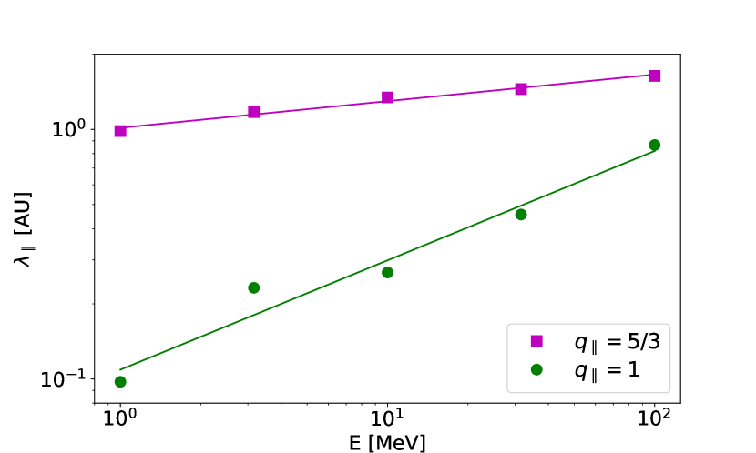
Figure 1: The parallel mean free path of protons at energies 1–100 MeV for turbulence with $\delta B^{2}/B^{2}=0.1$. The curves show the power-law fits to the mean free paths, with trends $E^{0.11}$ and $E^{0.44}$ for $q_{\parallel}=5/3$ and $1$, respectively.

The slab spectral index affects the particles’ parallel scattering mean free path, which from quasilinear theory (Jokipii, 1966) varies as $\lambda_{\parallel}\propto R^{2-q_{\parallel}}$, where $R$ is the particle rigidity. In addition, the turbulence energy for the spectra with the two slab spectral indices, $q_{\parallel}=5/3$ and $1$, results in a different scattering power at the resonant scales of the particles simulated in this study. We show $\lambda_{\parallel}$ as determined from the particle simulations in Figure 1, for the two spectral indices and $\delta B^{2}/B^{2}=0.1$. The trends of $\lambda_{\parallel}$ as function of proton energy for the two slab spectral indices, depicted with the fitted power law curves, with $E^{0.11}$ and $E^{0.44}$ for $q_{\parallel}=5/3$ and $1$, respectively, are consistent with the quasilinear theory result. The mean free paths presented in Figure 1 are consistent with those obtained using interplanetary turbulence properties (e.g. Pei et al., 2010; Laitinen et al., 2016; Strauss, Dresing & Engelbrecht, 2017) and SEP observation analysis (e.g. Palmer, 1982; Torsti, Riihonen & Kocharov, 2004).

We analyse the cross-field extent of the particle distribution as a function of the distance along the mean field direction, using

$$\sigma_{\perp}^{2}(z,t)=\left<(x(z,t)-\left<x(z,t)\right>)^{2}\right>$$ (2)

where $\left<\right>$ represents the ensemble average of particles. The use of $x$ instead of $y$ is arbitrary, and due to the axissymmetry of the turbulence has no effect on the obtained values. Also deviations in $r_{\perp}=\sqrt{x^{2}+y^{2}}$ could be considered, however it would complicate comparing our results with other work which typically consider cartesian deviations and diffusion coefficients. We note also that Equation (2) calculates the deviations with respect to the mean, $\left<x(z,t)\right>$, in order to eliminate the effects due to the potential asymmetries of the distributions (see Figures 2 and 3) that arise from finite range of fluctuation scales used in the simulations.

The form of the Equation (2) differs from the conventional definitions in that $\sigma_{\perp}^{2}(z,t)$ is defined for particles at a given field-parallel distance $z$ at time $t$, instead of for all particles in the simulation. This choice is motivated by observations: we do not observe the full 3D distribution of the particles, but rather sample the particle distribution in fixed points in space. Recent observations of SEPs by the STEREO, SOHO and ACE spacecraft have provided us with a view of the longitudinal extent of SEP events at 1 AU from the Sun. Our definition of $\sigma_{\perp}^{2}$ aims to provide comparison of simulated particle tranport with these measurements.

3 Results

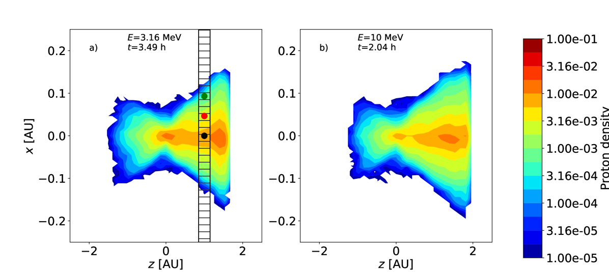
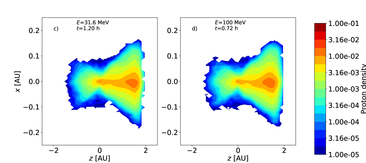
Figure 2: Contours of the spatial distributions of protons with energies of 3.16, 10, 31.6 and 100 MeV, with turbulence parameters $\delta B^{2}/B^{2}=0.1$ and $q_{\parallel}=5/3$. The contours are given at the times when an unscattered proton of the given energy would have propagated a distance of 2 AU. The circles in panel a) depict positions corresponding to curves in Figure 4, and the hatched box at 1 AU the region used for determining $\sigma_{\perp}^{2}(z=1~{}AU,t)$.

In this Section, we will first view the qualitative behaviour of the particle population along and across the mean field direction for different particle and turbulence parameters. We will then proceed to quantify the evolution of the particle population’s extent, using simple considerations presented in Appendix A.

As a first step in forming a view on the evolution of particle population along and across the mean field, we present a contour plot of the proton density in Figure 2, for turbulence with $\delta B^{2}/B^{2}=0.1$ and $q_{\parallel}=5/3$ for four different proton energies. The distributions are integrated in $y$-direction to reduce numerical noise in the contours. The distributions are shown at times when a non-scattered proton of the given energy would have propagated the distance of $z_{ns}=2$ AU, $t=z_{ns}/v$. Thus, the four panels depict the distribution of particles of different energies that would have travelled the same distance, unscattered, in a constant background magnetic field. The sharp decrease and narrowing of the particle distribution near $z_{ns}=2$ AU demonstrates the finite propagation distance of the particles and the longer distance travelled by particles along meandering field lines to larger cross-field distances in the $x$-direction. The decrease starts already before $z=2$ AU, as some of the first particles have experienced scattering due to the small-scale turbulence.

As can be seen in Figure 2, the particles spread rapidly from their point of origin in the cross-field direction (vertical axis): the front of the fastest propagation particles at $z=2$ AU is much wider than at $z=0$ AU. A small number of backscattered particles have advanced to the region $z<0$ AU (on horizontal axis), and show also expansion in the cross-field direction faster than that at $z=0$ AU. As discussed in Laitinen, Dalla & Marsh (2013), the resulting butterfly-shape of particle distribution cannot be obtained by a simple diffusive spreading of particles. In addition, the distribution of the particles at different distances along the field direction is qualitatively very similar at all energies. This suggests that the particles with different energies are propagating along the same pathways.

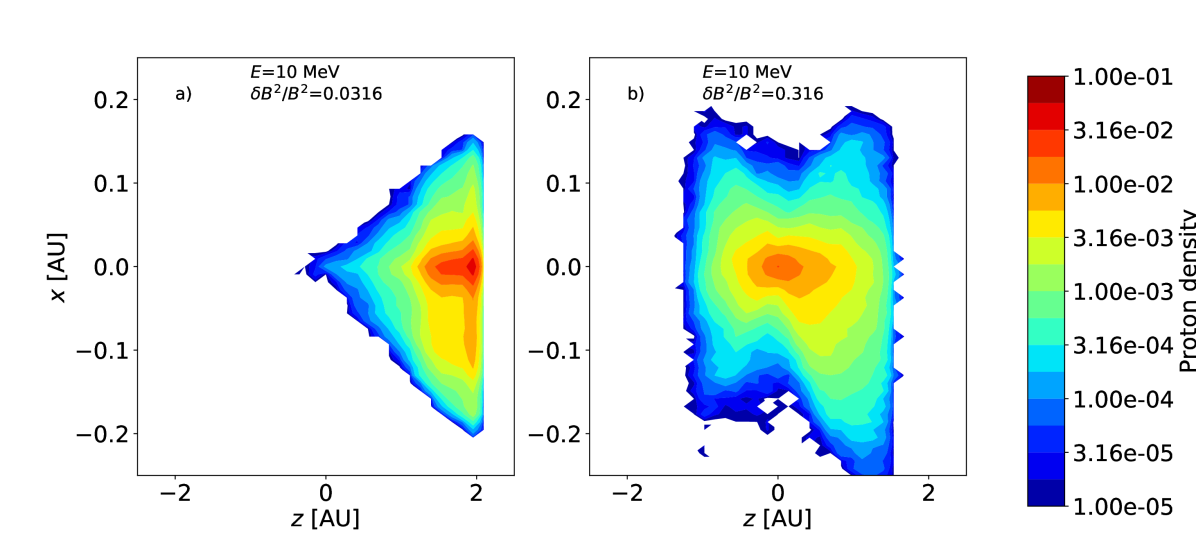
Figure 3: Contours of the spatial distributions of 10 MeV protons with turbulence amplitudes 0.00316 and 0.316, and $q_{\parallel}=5/3$. The contours are given at the time when the times when an unscattered proton of the given energy would have propagated a distance of 2 AU, at $t=2.04$ h.

In Figure 3, we show the distribution of 10 MeV protons in turbulence of different strength, $\delta B^{2}/B^{2}=0.0316$ and $\delta B^{2}/B^{2}=0.316$ in panels a) and b), respectively. The distributions are again shown at the time when an unscattered particle would have reached 2 AU along a uniform magnetic field. The distributions differ significantly at $z<0$ AU where the number of backscattered particles decreases as the turbulence weakens, with almost no backscattered particles for the weakest turbulence case, $\delta B^{2}/B^{2}=0.0316$ (Figure 3 a)). On the other hand, at $z\sim 2$ AU the particles propagating in weaker turbulence (3 a)) have progressed further in parallel direction, remaining in a more coherent pulse. These differences are due to the dependence of parallel scattering rate on the turbulence amplitude. For 10 MeV protons, the quasi-linear parallel mean free path, obtained from the simulated particles, is $\lambda_{\parallel}=0.29$ AU for the case of $\delta B^{2}/B^{2}=0.316$ (Figure 3 b)), consistent with considerable scattering along the mean magnetic field by the time the particles have propagated for a time time corresponding to scatter-free propagation of 2 AU. For the case of $\delta B^{2}/B^{2}=0.0316$, the mean free path is $\lambda_{\parallel}=7.6$ AU, resulting in the almost scatter-free propagation depicted in Figure 3 a). For the intermediate case, $\delta B^{2}/B^{2}=0.1$, depicted in Figure 2 b), the mean free path is $\lambda_{\parallel}=1.3$ AU, which can be seen in some parallel diffusion and backscattering of the particles.

The cross-field extent of the particle distribution also appears to depend on the turbulence amplitude, as seen when comparing Figures 3 a), 2 b) and 3 b), for the weak, intermediate and strong scattering conditions, respectively, for 10 MeV protons. The distribution is clearly narrower at lower turbulence amplitude turbulence at $z=0$ AU. A similar trend is seen also at larger distances along the mean field line direction: at $z=2$ AU, the weak turbulence case, as presented in Figure 3 a), the particles are much more concentrated on a narrow cross-field extent than in the more turbulent cases presented in Figures 2 b) and 3 b).

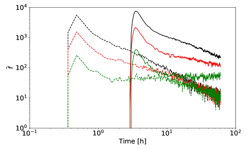
Figure 4: The time evolution of the distribution of protons at $z=1$ AU and $x=0,$ 0.046 and 0.093 AU from (black, red and green curves, respectively), for 1 and 100 MeV (solid and dashed curves, respectively), and $\delta B^{2}/B^{2}=0.1$ and $q_{\parallel}=5/3$.

In Figure 4, we show the time development of the particle density, as it would be measured by spacecraft situated at the black, red and green circles in Figure 2 a), for 1 and 100 MeV protons (solid and dashed curves), respectively. As can be seen, the particle density decreases strongly when the measuring point is moved from the black circle, connected along the mean magnetic field to the particle source, across the mean field direction, to the red and green circles. However, the ratio of intensities at different locations appears to be initially independent of time (at times $<$ 1 h for 100 MeV protons, and $<$ 10 h for 1 MeV protons), and only at later times the intensities at different locations begin to converge. This behaviour of initially time-independent cross-field distribution is seen at both energies in Figure 4. Furthermore, the temporal behaviour in the initial phase of the simulations, when scaled with the particle velocity, is very similar. Thus, the initial cross-field spreading of the particles seems to be independent of both energy and velocity-scaled time. At later times, the intensities at different locations begin to converge, as the width of the particle population increases.

To analyse the particle cross-field extent quantitatively, we study the temporal evolution of the cross-field variance of the particles, $\sigma_{\perp}^{2}(z,t)$, as a function of time at different distances from the particle source. As discussed in the previous section, we define the cross-field variance for particles at a given distance along the mean field direction using Equation (3), so that for example the variance $\sigma_{\perp}^{2}(z=1\mathrm{AU},t=3.49\mathrm{h})$ is determined from the particles within the hatched box in Figure 2 a).

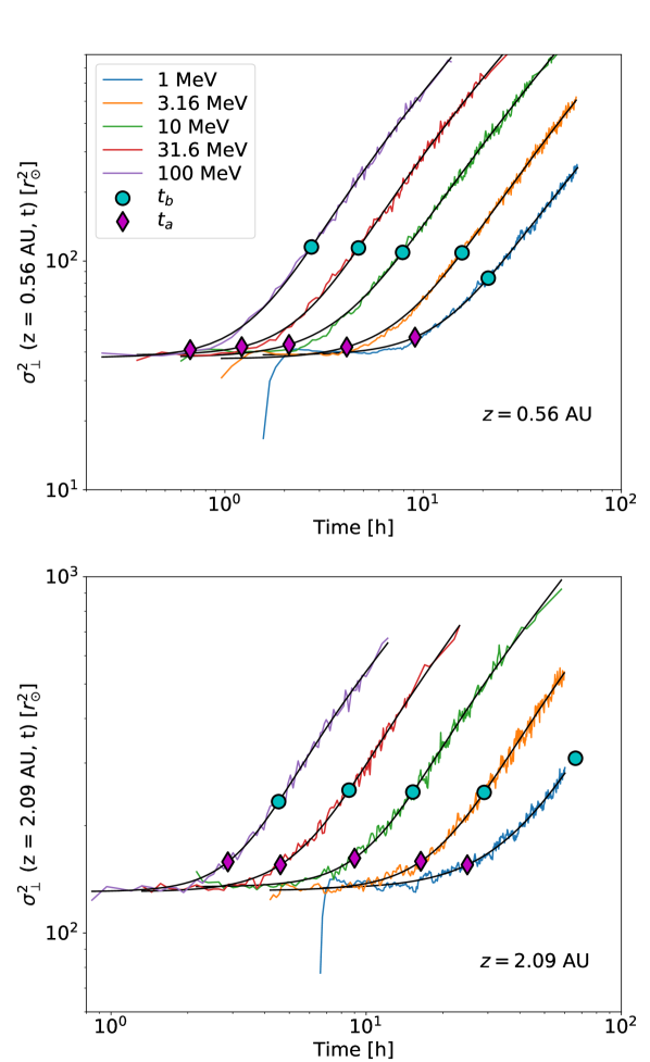
Figure 5: The mean square width of protons at 0.56 AU (top panel) and 2.09 AU along the mean field direction from the source location. The black curves show fits made using Equation 3, the magenta diamond the time $t_{a}$ and the cyan circle the time $t_{b}$. The turbulence parameters are $\delta B^{2}/B^{2}=0.1$ and $q_{\parallel}=5/3$.

In Figure 5, we show $\sigma_{\perp}^{2}(z,t)$ at $z=$0.56 AU (top panel) and $z=$2.09 AU (bottom panel), as a function of time, for 1, 3.16, 10., 31.6 and 100 MeV protons, from right to left, respectively. The black curves represent a fitted function that is discussed below. As we can see, the temporal behaviour of the cross-field variance of the particles can be decomposed to three time periods. The first time period, visible only for 1 MeV protons in Figure 5 (blue, rightmost curve) demonstrates fast increase of the variance to a constant level (at times $<2$ h in the top panel). This is caused by the fact that the particles with very small cross-field deviation are likely to have the shortest path-lengths along the meandering field lines, and thus the first particles will arrive earlier to the well-connected location ($x=0$ AU in Figures 2 and 3) than to larger cross-field deviations. The effect of the length of the meandering fieldlines on the particle onsets at different spatial locations will be investigated in a separate study.

The first time period is short, and due to finite time sampling of the particle locations within the simulations, it is not visible at higher energies. After the initial fast rise, the variance remains at a constant level for a considerably long time, at about $\sigma_{\perp}^{2}(z,t)=38\;\mathrm{r}_{\odot}^{2}$ at z=0.56 AU, and $130\;\mathrm{r}_{\odot}^{2}$ at z=2.09 AU. The constant level is independent of energy, and increases with distance along the mean magnetic field direction (top vs bottom panel of Figure 5).

Subsequently, the cross-field extent of the particle population begins to increase and finally reaches a time-asymptotic $\sigma_{\perp}^{2}\propto t$ trend, consistent with diffusive cross-field spreading of the particles. Both the onset time and the time profile of the change from constant to the diffusive phase depend on both the particle energy and the distance along the $z$ axis. The simplest method of obtaining the time when the cross-field diffusion becomes significant, $t_{a}$, is to use time at which the time-asymptotic straight line $\sigma_{\perp}^{2}\propto t$ intersects the initial constant value of $\sigma_{\perp}^{2}$ level (the magenta and black dashed lines in Figure 9, respectively).

The simplest approach to describe mathematically the temporal behaviour of the cross-field variance presented in Figure 5 would be to consider a diffusive spreading of particles from the meandering field lines with constant diffusion coefficient, which would result in variance given by Equation (8). While such a model is easy to implement and can be used as the first approach, as in, e.g., Laitinen et al. (2016), we will consider here an improvement to the modelling of the transition, based on the work by Laitinen & Dalla (2017). In Appendix A, we derive a model with time-dependent diffusion coefficient, which will justify fitting the variance with functional forms such as Equation (9). In this work, we will use

$$\sigma_{\perp}^{2}(z,t)=\sigma_{\perp 0}^{2}(z)+\frac{\sigma_{\perp 1}^{2}(z)\,t/t_{0}}{1+\left[t_{b}(z)/t\right]^{\alpha(z)-1}}.$$ (3)

where $\sigma_{\perp 0}^{2}(z)$ is the early-time constant cross-field variance of the particles at distance $z$, $t_{0}=1$ h the unit of time, $t_{b}(z)$ is the onset time of the time-asymptotic diffusive regime, and $\alpha(z)$ the power law index that describes the fast spreading of the particle population before $t_{b}$. The time-asymptotic diffusive rate of change of the cross-field variance of the particle population is given by $\sigma_{\perp 1}^{2}(z)/t_{0}\equiv 2\,\kappa_{\perp}(t\gg t_{b})$, with $\kappa_{\perp}(t)$ the time-dependent particle diffusion coefficient (see Appendix A). Using the parameters in Equation (3), $t_{a}=\sigma_{\perp 0}^{2}/\sigma_{\perp 1}^{2}\;t_{0}$. The times $t_{a}$ and $t_{b}$, and their relation to the $\sigma_{\perp}^{2}(z,t)$ curve and its asymptotes are shown in Figure 9, and are further discussed in Appendix A.

It should be noted that Equation (3) is of the same form as the fitting function used in Laitinen & Dalla (2017), at the limit of $t\gg t_{1}$ in their formulation. Here, we exclude the early behaviour, $t\lesssim t_{1}$ discussed in Laitinen & Dalla (2017), as displacements of order Larmor radius are too small to be seen in our current analysis.

We fit Equation (3) to the cross-field variances from our simulations at different distances $z=$0.3–3 AU, and study the dependence of the fit parameters on $z$, the particle energy and the turbulence properties. We exclude fits where the relative error of any of the fit parameters in Equation (3) exceeds 10%. As an example, we show the fits of the simulation results with Equation (3) in Figure 5 with black curves, with $t_{b}$ shown with a cyan circle. As can be seen, Equation (3) mostly fits the simulation results well at all energies on both locations.

In Figure 6, we show the evolution of the fit parameters as a function of $z$ for five proton energies for turbulence parameters $\delta B^{2}/B^{2}=0.1$ and $q_{\parallel}=5/3$. Panel a) shows the early-time constant cross-field variance $\sigma_{\perp 0}^{2}$, which increases approximately linearly as a function of distance. The $\sigma_{\perp 0}^{2}(z)$ curves for different energies overlay each other almost perfectly, suggesting that the spread of particles is caused by the diffusive spreading of the meandering magnetic field lines, rather than particle scattering in space across the mean field.

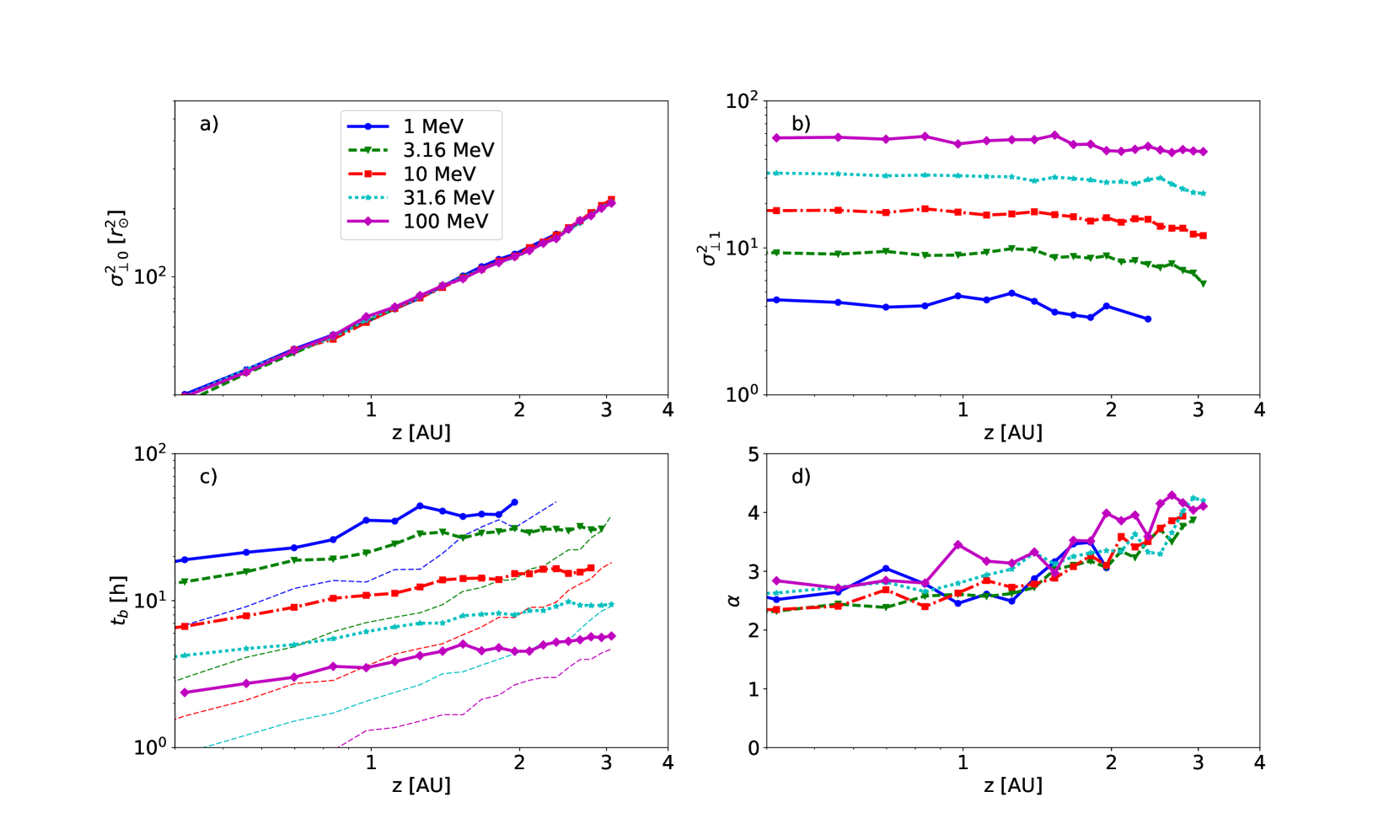
Figure 6: The fitting parameters of the Equation (3) to the cross-field particle distribution variances at different distances, for protons of energies 1–100 MeV propagating in turbulence with $\delta B^{2}/B^{2}=0.1$ and $q_{\parallel}=5/3$. a) The early-time cross-field variance of the distribution, $\sigma_{\perp 0}^{2}$; b) the asymptotic long-time behaviour $\sigma_{\perp 1}^{2}$; c) The turnover time $t_{b}$ (thick curves) and the asymptotic behaviour changing time $t_{a}$ (thin dashed curves); d) The power law index $\alpha$.

In Figure 6 b), we show $\sigma_{\perp 1}^{2}$, which describes the time-asymptotic diffusive spreading rate of the particles. As can be seen, $\sigma_{\perp 1}^{2}$ is clearly energy-dependent, and almost independent of $z$, as expected for diffusive spreading of particles. We determined that $\sigma_{\perp 1}^{2}$ is roughly proportional to the particle velocity, and is also consistent with the theoretical dependence $\kappa_{\perp}\propto R^{10/9}$ of the particle diffusion coefficient on rigidity (Matthaeus et al., 2003; Shalchi, Bieber & Matthaeus, 2004).

In Figure 6 c), we show $t_{b}$, which represents the onset time of the diffusive spreading of particles. A closer inspection shows that the onset time is roughly proportional to the inverse of velocity. Similar scaling was found by Laitinen & Dalla (2017), who noted that the transition timescale from the slow to fast diffusive spreading at $z=0$ AU is proportional to the parallel scattering timescale $\tau_{\parallel}\propto v^{-2/3}$.

However, as can be seen in Figure 6, the onset time $t_{b}$ is not independent of the distance $z$, but increases slowly, inconsistent with the assumptions of the simple diffusion model described in Equation (9). The inconsistency can be caused by the finite propagation time of the particles to distance $z$, not taken into account in Equation (9).

In Figure 6 c), we also show the asymptotic time $t_{a}$, with the thin dashed curves. As can be seen, $t_{a}$ approaches and surpasses $t_{b}$ at larger distances. As discussed in Appendix A, the determination of $t_{b}$ and $\alpha$ are unreliable when $t_{a}$ approaches $t_{b}$, and the unreliable values of $t_{b}$ are not shown in Figure 6 c).

Figure 6 d) shows the parameter $\alpha$, which describes the fast spreading of the particles until the time-asymptotic diffusive phase is reached. As interpreted by Laitinen & Dalla (2017), the fast spreading begins when the particles cease being well tied to their field lines. The onset time of the fast spreading phase, denoted by $t_{1}$ in Laitinen & Dalla (2017), however, is masked by the early-time $\sigma_{\perp 0}^{2}$ (see Figure 5), and can only be quantified using the method described in Laitinen & Dalla (2017). The $\alpha$ in Figure 6 d) shows no clear energy dependence, consistent with Laitinen & Dalla (2017).

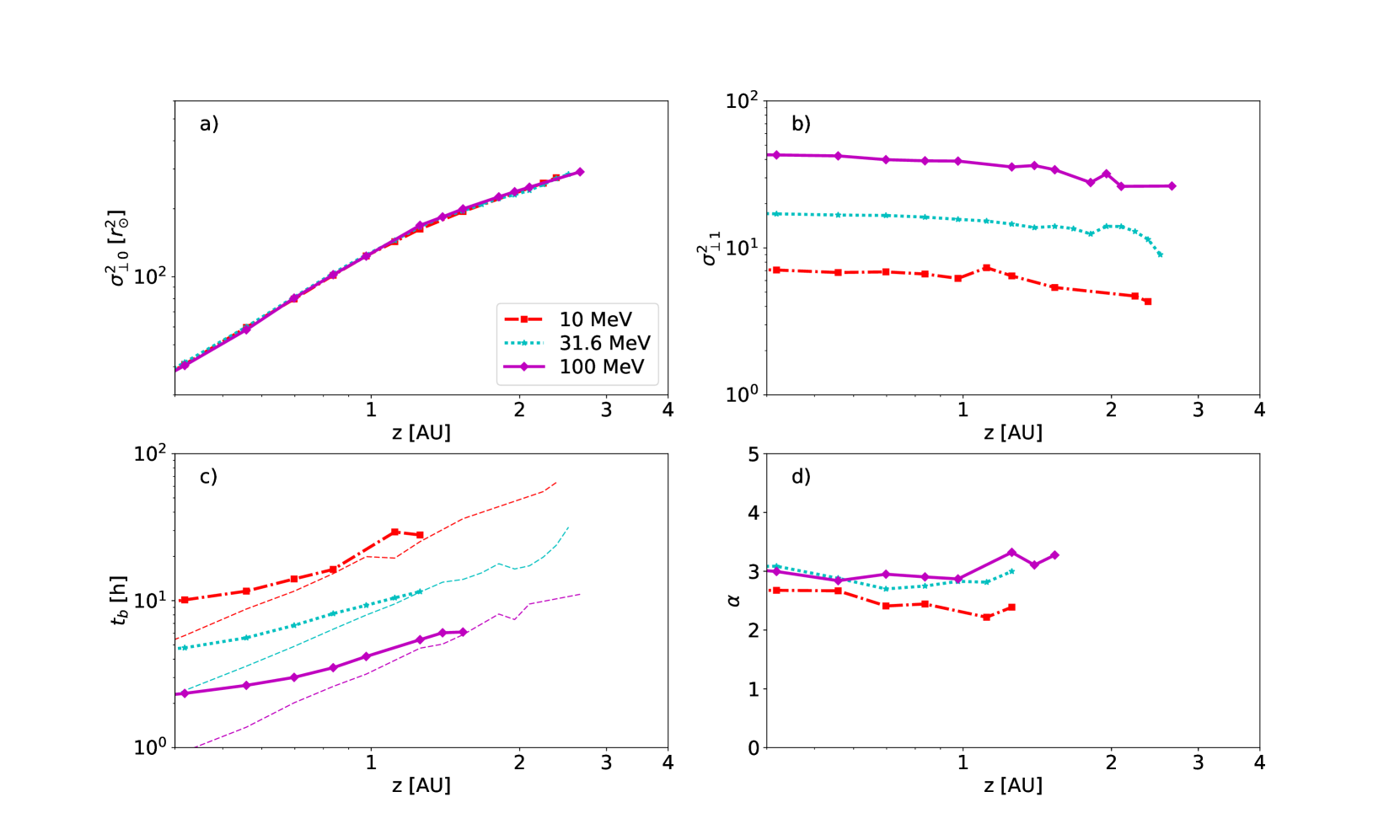
Figure 7: The fitting parameters of the Equation (3) to the cross-field particle distribution variances at different distances, for proton energies 10–100 MeV propagating in turbulence with $\delta B^{2}/B^{2}=0.1$ and $q_{\parallel}=1$. a) The early-time cross-field variance of the distribution, $\sigma_{\perp 0}^{2}$; b) the asymptotic long-time behaviour $\sigma_{\perp 1}^{2}$; c) The turnover time $t_{b}$ (thick curves) and the asymptotic behaviour changing time $t_{a}$ (thin dashed curves); d) The power law index $\alpha$.

In Figure 7, we show the simulation fit parameters for particles in turbulence with slab spectral index $q_{\parallel}=1$. The fit of the variance with Equation (3) could be successfully performed only for energies in the range E=10-100 MeV. For lower energy protons, the cross-field variance remained almost constant for the simulation period of 60 hours.

In panel a) we can see that the early-time, constant cross-field variance $\sigma_{\perp 0}$ is independent of energy also for $q_{\parallel}=1$. This energy-independence was evident also for energies $<10$ MeV, for which the fitting of Equation (3) was not successful. In panel b), we note that $\sigma_{\perp 1}^{2}$ is again almost independent of $z$. However, its dependence on energy is different than in the case $q_{\parallel}=5/3$ (Figure 6 b)): the dependence is now close to $\sigma_{\perp 1}^{2}\propto p^{1.5}$. This dependence is again close to the NLGC prediction $\lambda_{\perp}\propto\lambda_{\parallel}^{1/3}$ which, together with the quasilinear theory result $\lambda_{\parallel}\propto R^{2-q_{\parallel}}$ and $q_{\parallel}=1$ gives $\kappa_{\perp}=v\lambda_{\perp}/3\propto p^{4/3}$ at non-relativistic limit (Matthaeus et al., 2003; Shalchi, Bieber & Matthaeus, 2004).

In panel c) of Figure 7, we show the behaviour of the onset time $t_{b}$ as a function of energy and distance. Compared to the $q_{\parallel}=5/3$ case, the dependence of the onset time on energy is stronger, with $t_{b}\propto 1/v^{3/2}$. This is in contradiction with the suggestion that the timescale would scale as the parallel scattering time (Laitinen & Dalla, 2017), as this timescale, $\lambda_{\parallel}/v$, would be constant for $q_{\parallel}=1$. The discrepancy may be due to the strong parallel scattering of the particles for the $q_{\parallel}=1$ case. In a strongly diffusive environment, the particles propagate in timescales $t\propto z^{2}$, thus much slower for the scatter-dominated case of $q_{\parallel}=1$, as compared to the almost scatter-free case with $q_{\parallel}=5/3$. The slower parallel propagation implies that the finite propagation time effects, not accounted for in the simple diffusion model, are much more pronounced for the $q_{\parallel}=1$ case.

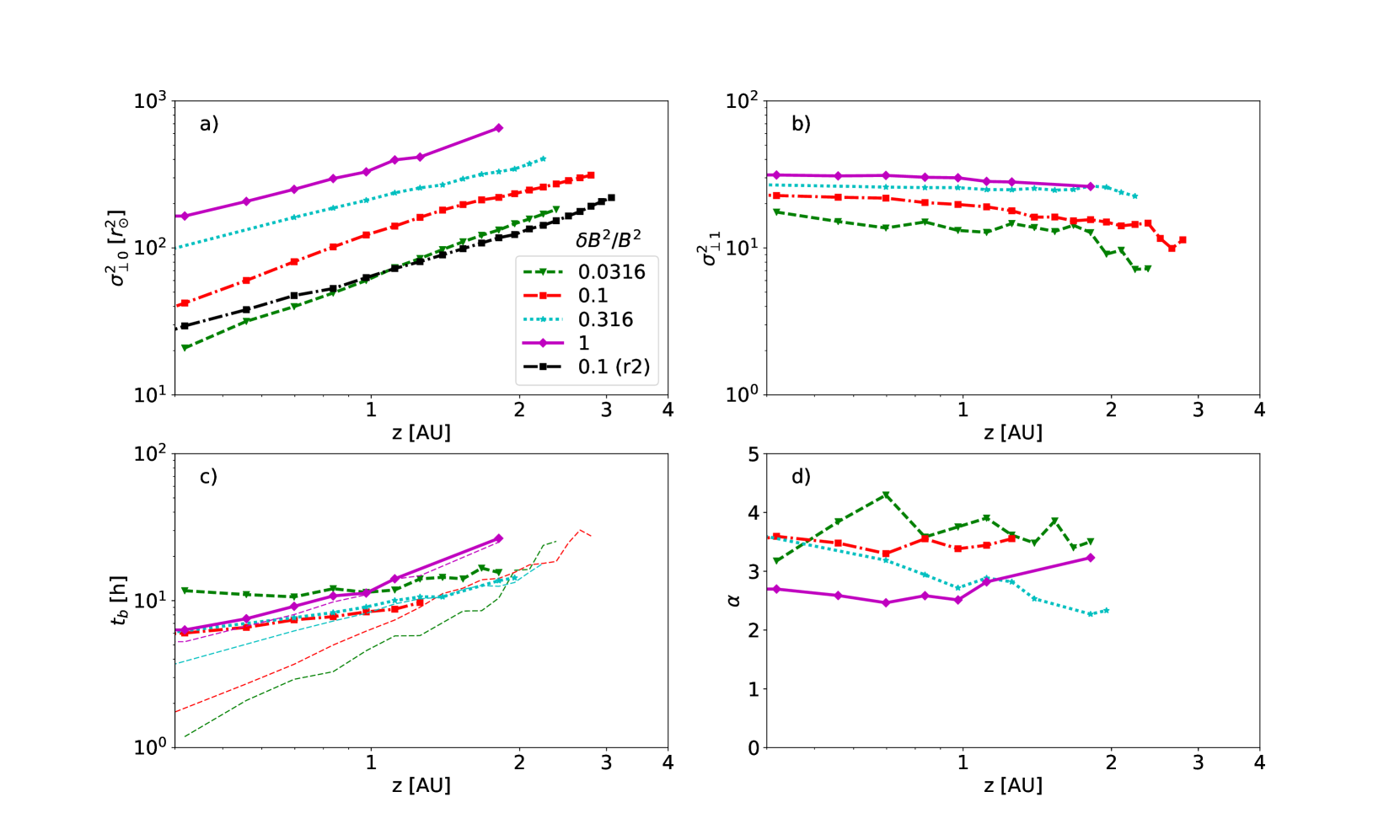
Figure 8: The fitting parameters of the Equation (3) to the 10 MeV proton cross-field variances at different distances propagating in turbulence with different amplitudes amplitudes $\delta B^{2}/B^{2}$ and $q_{\parallel}=5/3$. a) The early-time cross-field variance of the distribution, $\sigma_{\perp 0}^{2}$, with the black dash-dotted curve showing a different turbulence realisation as compared to the red dash-dotted curve, for $\delta B^{2}/B^{2}=0.1$; b) the asymptotic long-time behaviour $\sigma_{\perp 1}^{2}$; c) The turnover time $t_{b}$ (thick curves) and the asymptotic behaviour changing time $t_{a}$ (thin dashed curves); d) The power law index $\alpha$.

In Figure 8, we investigate the effect of varying turbulence amplitudes on the 10 MeV proton distribution extent across the mean field, with $q_{\parallel}=5/3$, in the same format as in Figures 6 and 7. The turbulence at different amplitudes is obtained so that the random phases and polarisations of the Fourier modes were the same for each simulation, and only the amplitudes of the Fourier modes were changed.

Figure 8 a) shows the dependence of the early-time constant cross-field extent $\sigma_{\perp 0}^{2}$ on the turbulence amplitude, from $\delta B^{2}/B^{2}=0.0316$ (dashed green curve) to $\delta B^{2}/B^{2}=1$ (solid magenta curve). The initial variance is proportional to the distance $z$ along the mean field direction at all turbulence amplitudes, again consistent with particles propagating on diffusively meandering field lines. We found that $\sigma_{\perp 0}^{2}/z\propto\sqrt{\delta B^{2}/B^{2}}$, which is consistent with the dependence of the field line diffusion coefficient on the amplitude of the 2D-turbulence (Matthaeus et al., 1995).

In Figure 8 a) we also show the early-time cross-field variance $\sigma_{\perp 0}^{2}$ for a simulation with $\delta B^{2}/B^{2}=0.1$ with random phases and polarisations different from the ones used in the other simulations presented in Figure 8, with black dash-dotted curve. As can be seen, the two realisations with $\delta B^{2}/B^{2}=0.1$ (black and red dash-dotted curves) differ by factor 2. Thus, different realisations can locally produce significantly different turbulence conditions, which can affect parametric comparison of particle and field line dynamics in simulated turbulence. For this reason, it is important to keep consistency in the simulated fields when comparing, e.g., the effect of turbulence ampitudes only on the particle transport, as in Figure 8.

In Figure 8 b) we see that the time-asymptotic diffusive spreading rate does not depend strongly on the turbulence amplitude. Upon closer inspection, we find that $\sigma_{\perp 1}^{2}$ from our fits is proportional to $(\delta B^{2}/B^{2})^{0.25}$, which is slightly flatter than the dependence given by the NLGC value $\kappa_{\perp}\propto(\delta B^{2}/B^{2})^{2/3}\kappa_{\parallel}^{1/3}$ (Shalchi, Bieber & Matthaeus, 2004), which for quasilinear theory $\kappa_{\parallel}\propto(\delta B^{2}/B^{2})^{-1}$ (Jokipii, 1966) would give $\kappa_{\perp}\propto(\delta B^{2}/B^{2})^{1/3}$. In our simulations, the dependence of $\kappa_{\parallel}$ on turbulence amplitude, however, differed slightly from the quasilinear theory value: using our $\kappa_{\parallel}$ from the simulations in the NLGC expression we get $\kappa_{\perp}\propto(\delta B^{2}/B^{2})^{0.2}$, close to the $\sigma_{\perp 1}^{2}\propto(\delta B^{2}/B^{2})^{0.25}$ obtained from our fits in Figure 8 b). In addition, the recent work by Ruffolo et al. (2012) found a non-power law, flattening behaviour for $\kappa_{\perp}$ at higher turbulence amplitudes, which may be visible also in our simulations.

In Figure 8 c), we see that $t_{b}$ decreases with increasing turbulence amplitude for the two lowest turbulence amplitudes (the green dashed curve and red dash-dotted curve), again consistent with the Laitinen & Dalla (2017) result. Subsequently, at higher amplitudes, the onset time begins to increase. The increase can in part be due to slow propagation times of the more diffusive particles in higher-amplitude turbulence, as well as due to the asymptotic time $t_{a}$ (the thin dashed curves) approaching $t_{b}$ which, as discussed in Appendix A, renders the fitting of the variance to Equation (3) insensitive to the parameters $t_{b}$ and $\alpha$. The resulting spurious behaviour can also be seen in the fitted value of the power law index $\alpha$ in Figure 8 d).

4 Discussion

Our analysis shows that the initial cross-field propagation of particles in turbulent magnetic fields is non-diffusive over a wide range of turbulence and particle parameters, reinforcing the conclusions made in the case study by Laitinen, Dalla & Marsh (2013). Initially particles remain on their field lines, as demonstrated by the energy-independent initial spreading of the particles in different turbulence environments (Figures 6 a) and 7 a)), which is followed by a time-asymptotic, energy-dependent diffusive spreading of the particles across the mean field direction. The early-time constant cross-field variance phase is seen as a very fast access of particles to wide cross-field ranges, and it lasts for hours to tens of hours depending on particle and turbulence parameters.

We found that the early-time cross-field extent of the particle population, as given by the cross-field variance $\sigma_{\perp 0}^{2}$ in Equation (3), is proportional to the distance $z$ from the particle source along the mean field direction, and $\sqrt{\delta B^{2}/B^{2}}$. Thus, the initial propagation phase is consistent with particles propagating along diffusively meandering field lines in turbulence dominated by 2D wave modes (Matthaeus et al., 1995). At the time-asymptotic limit, the rate of cross-field spreading obtained in our simulations can be described as diffusion with cross-field diffusion coefficient $\kappa_{\perp}$ proportional to velocity (for the $q_{\parallel}=5/3$ case) and $(\delta B^{2}/B^{2})^{0.25}$, consistent with the our current theoretical understanding of asymptotic particle cross-field diffusion (e.g. Matthaeus et al., 2003; Shalchi, Bieber & Matthaeus, 2004; Ruffolo et al., 2012). Thus, the early-time and the time-asymptotic phases of the particle cross-field propagation in our simulations are consistent with our theoretical understanding of the field line and particle behaviour at the corresponding limits.

Our study shows that the transition between the early spreading along the meandering field lines, and the time asymptotic diffusion phase does not follow the simple diffusion picture presented in Equation (8) in most cases studied in this work, but suggests a delayed onset of the diffusion phase after fast expansion, as indicated by the recent results by Laitinen & Dalla (2017). As discussed in Appendix A, assuming particles to diffuse from the meandering field lines at a constant rate (magenta curve in Figure 9) can result in overestimation of the cross-field variance of the particle population by up to a factor of 2 during the transition phase between the initial and time-asymptotic propagation phases. We find that for low-scattering conditions, the onset of the time-asymptotic phase, $t_{b}$, follows approximately the dependence on the parallel scattering rate obtained by (Laitinen & Dalla, 2017). For stronger tubulence, however, the scaling does not hold any more, possibly due to finite propagation time effects, which are not contained in our simple model behind the formulation of Equation (3). The particles may have also been already decoupled from their fieldlines before reaching distance $z$, which would result in inaccuracy in the determination of $t_{b}$, as discussed in the Appendix A.

5 Conclusions

In this work, we have studied how the turbulence and particle properties affect the particle spreading across the mean field direction early after the particle release. Our results show that

• Initially, the particles spread systematically and rapidly to a wide cross-field range along meandering field lines. They remain on the fieldlines from hours up to tens of hours for protons of 1–100 MeV, in turbulence consistent with proton parallel mean free paths $\lambda_{\parallel}\sim 0.1-1$ AU, range consistent with those measured during solar energetic particle events (e.g. Palmer, 1982; Torsti, Riihonen & Kocharov, 2004) and interplanetary turbulence conditions (r.g. Pei et al., 2010; Laitinen et al., 2016; Strauss, Dresing & Engelbrecht, 2017).

• The late-time behaviour of the particles is consistent with energy-dependent cross-field diffusion, and is consistent with the current theoretical understanding of the time-asymptotic cross-field diffusion of particles in turbulent magnetic fields (e.g. Matthaeus et al., 2003; Shalchi, Bieber & Matthaeus, 2004; Ruffolo et al., 2012).

• The transition between the initial and time-asymptotic behaviour can be roughly modelled as a simple spatial diffusion of particles from their meandering field lines. More precise modelling reveals a delayed decoupling of particles from the meandering field lines, as demonstrated in Laitinen & Dalla (2017).

Thus, our study shows that over a wide range of turbulence and particle parameters SEP cross-field propagation cannot be modelled by cross-field diffusion alone early in the SEP event, but the systematic propagation along meandering field lines must be taken into account. Simple models, such as the one applied in Laitinen et al. (2016), which model the particle distribution evolution as cross-field diffusion of particles from meandering field lines provide a significant improvement as compared to the earlier models diffusing particles with respect to the mean magnetic field. Future fully consistent cross-field propagation models should also include the timescales related to the decoupling of the particles from the meandering field lines (Laitinen & Dalla, 2017). For early-time evolution of the particle populations, a time-dependent diffusion coefficient, such as used in Equation (9), may prove useful. We will investigate advanced modelling of cross-field particle propagation in a future work.

Appendix A The width of a distribution in a simple diffusion picture

If we exclude the finite propagation time effects on particle propagation, the diffusive spreading of a particle population along and across the mean field can be described as spatial diffusion as

$$\frac{\partial n_{3D}}{\partial t}=\nabla\cdot\hat{\kappa}\nabla n_{3D}$$ (4)

where $n_{3D}$ is the density of the particles, and the non-zero elements of the diffusion tensor $\hat{\kappa}$ are $\kappa_{xx}=\kappa_{yy}\equiv\kappa_{\perp}$ and $\kappa_{zz}\equiv\kappa_{\parallel}$. For impulsive point-source injection, the solution to the diffusion equation is

$$n_{\mathrm{3D}}(r,t)=\frac{I_{0}}{\left(4\kappa_{\perp}^{2}\kappa_{\parallel}t\right)^{3/2}}\exp\left\{-\frac{x^{2}+y^{2}}{4\kappa_{\perp}t}-\frac{z^{2}}{4\kappa_{\parallel}t}\right\}.$$ (5)

Taking the second moment of this with respect to $x$, we find for the variance in the x direction

$$\sigma_{x}^{2}(t,y,z)=2\kappa_{\perp}t$$ (6)

Thus, for an impulsive injection and pure diffusion, the variance of the particle population at all $z$ grows linearly with time.

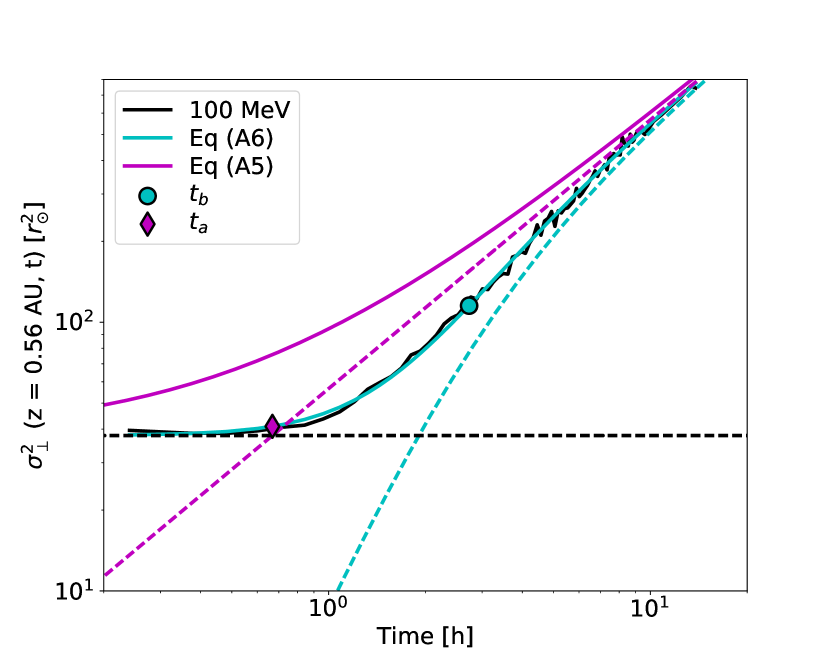
Figure 9: The cross-field variance of 100 MeV protons at 0.56 AU, with turbulence parameters $\delta B^{2}/B^{2}=0.1$ and $q_{\parallel}=5/3$. The solid magenta curve shows the fit to Equation (8) and the solid cyan curve to Equation (9), using the functional shape given in Equation 3. The black dashed line shows the asymptotic $\sigma_{\perp}^{2}(t,z)=\sigma_{\perp 0}$, the dashed cyan curve the second term in Equation (3), and the dashed magenta curve the asymptotic $\sigma_{\perp}^{2}(t,z)=\sigma_{\perp 1}t/t_{0}$. The magenta diamond shows the intercept of the asymptotes, $t_{a}=\sigma_{\perp 0}/\sigma_{\perp 1}t_{0}$, and the cyan circle shows the $t_{b}$.

Laitinen, Dalla & Marsh (2013) showed that cross-field diffusion does not describe the particle cross-field distribution early in the event and concluded that the particles follow the meandering field lines systematically, and diffuse from them slowly. To describe such behaviour, we consider as the first approach a simple model where the particles are initially distributed in the cross-field $x$-direction on a Gaussian distribution with $\sigma^{2}=2\,z\,D_{FL}$, where $D_{FL}$ is the diffusion coefficient for the field lines, mimicking the cross-field distribution of particles of particles that propagate along turbulently meandering field lines. Subsequently, the particles spread diffusively in the $x$-direction from their field lines. As we ignore the propagation along the field lines in this simple model, we can describe the evolution of the particle density as

$$\frac{\partial n_{1D}(x,z,t)}{\partial t}=\frac{\partial}{\partial x}\kappa_{\perp}\frac{\partial n_{1D}(x,z,t)}{\partial x}$$ (7)

which, for the Gaussian initial condition yields for the cross-field variance

$$\sigma_{\perp}^{2}(t,z)=2\,z\,D_{FL}+2\kappa_{\perp}t.$$ (8)

We show the behaviour of the cross-field variance given by Equation (8) in Figure 9 with the solid magenta curve, comparing it with a simulation case with 100 MeV protons at 0.56 AU along the mean field direction, with turbulence variance $\delta B^{2}/B^{2}=0.1$ and $q_{\parallel}=5/3$. The first and second term in Equation (8) are shown with the black and magenta dashed curves, respectively, and the intercept time of the terms, $t_{a}$, shown with the magenta diamond. As can be seen, the magenta curve does not trace the simulation result, solid black curve, well during the transition phase.

Recently, Laitinen & Dalla (2017) noted that the decoupling of particles from their initial field lines is initially slow, and only at later times rapidly converges to the time-asymptotic diffusion trend. Such a behaviour can be mimicked by allowing time-dependence for the particle diffusion coefficient, with $\kappa_{\perp}(t)=\kappa_{\perp 0}\,T(t)$. Substituting $\mathrm{d}\tau=T(t)\mathrm{d}t$ we can solve the Equation (7) for $\kappa_{\perp}(t)$, which results, for impulsive point source, in variance $\sigma_{x}^{2}(t)=2\kappa_{\perp 0}\tau(t)$, and for a Gaussian initial condition in

$$\sigma_{\perp}^{2}(t,z)=2\,z\,D_{FL}+2\kappa_{\perp 0}\tau(t).$$ (9)

We demonstrate the use of the solution given by Equation (9), parametrised as in Equation(3), in Figure 9, for the simulated case of 100 MeV protons at 0.56 AU along the mean field direction. turbulence variance $\delta B^{2}/B^{2}=0.1$ and $q_{\parallel}=5/3$. As can be seen, the Equation (9) describes the time evolution of the simulation results well.

When fitting the $\sigma_{\perp}^{2}(z,t)$ from the simulations to Equation (3), the difference between the simple approach, Equation (6), and Equation (3), is not always as clear as in Figure 9. If the $t_{b}\ll t_{a}$, the second term in Equation (3) approaches $\sigma_{\perp 1}^{2}(z)\,t/t_{0}$, and is longer sensitive to parameters $t_{b}$ and $\alpha$. The $t_{b}\ll t_{a}$ implies that the onset of the diffusive phase has taken place before the particles have reached the distance $z$.

To avoid showing the spurious fit parameters, we show the fit parameters $t_{b}$ and $\alpha$ only when $t_{b}\geq t_{a}$ in Figures 6, 7 and 8.

References

- Cohen et al. (2014) Cohen C. M. S., Mason G. M., Mewaldt R. A., Wiedenbeck M. E., 2014, ApJ, 793, 35
- Dresing et al. (2014) Dresing N., Gómez-Herrero R., Heber B., Klassen A., Malandraki O., Dröge W., Kartavykh Y., 2014, A&A, 567, A27
- Dresing et al. (2012) Dresing N., Gómez-Herrero R., Klassen A., Heber B., Kartavykh Y., Dröge W., 2012, Sol. Phys., 281, 281
- Dröge et al. (2010) Dröge W., Kartavykh Y. Y., Klecker B., Kovaltsov G. A., 2010, ApJ, 709, 912
- Fraschetti & Jokipii (2011) Fraschetti F., Jokipii J. R., 2011, ApJ, 734, 83
- Giacalone & Jokipii (1999) Giacalone J., Jokipii J. R., 1999, ApJ, 520, 204
- Giacalone & Jokipii (2012) Giacalone J., Jokipii J. R., 2012, ApJL, 751, L33
- He, Qin & Zhang (2011) He H.-Q., Qin G., Zhang M., 2011, ApJ, 734, 74
- Jokipii (1966) Jokipii J. R., 1966, ApJ, 146, 480
- Laitinen & Dalla (2017) Laitinen T., Dalla S., 2017, ApJ, 834, 127
- Laitinen, Dalla & Kelly (2012) Laitinen T., Dalla S., Kelly J., 2012, ApJ, 749, 103