Cyclotron transitions of bound ions

Abstract

A charged particle in a magnetic field possesses discrete energy levels associated with particle’s rotation around the field lines. The radiative transitions between these levels are the well-known cyclotron transitions. We show that a bound complex of particles with a non-zero net charge displays analogous transitions between the states of confined motion of the entire complex in the field. The latter bound-ion cyclotron transitions are affected by a coupling between the collective and internal motions of the complex and, as a result, differ from the transitions of a “reference” bare ion with the same mass and charge. We analyze the cyclotron transitions for complex ions by including the coupling within a rigorous quantum approach. Particular attention is paid to comparison of the transition energies and oscillator strengths to those of the bare ion. Selection rules based on integrals of collective motion are derived for the bound-ion cyclotron transitions analytically, and the perturbation and coupled-channel approaches are developed to study the transitions quantitatively. Representative examples are considered and discussed for positive and negative atomic and cluster ions.

I Introduction

Cyclotron radiation is a well-known phenomenon associated with the motion of a charged particle in a magnetic field. The particle rotates around the field lines and can thereby emit or absorb radiation of the frequency of rotation LanLif_1981 . The corresponding energy is the cyclotron energy given for a non-relativistic particle by the relation

$$\Omega=|Q|B/M,$$ (1)

where $Q$ and $M$ are the particle’s charge and mass, respectively, and $B$ is the strength of the magnetic field. We assume the field to be uniform and adopt the atomic system of units in which the unit of magnetic field strength is $2.3554\times 10^{5}$ T.

For a stuctureless (bare) ion, such as an atomic nucleus, the properties of the cyclotron transitions are fully determined by the ion’s mass and charge. A complex ion (i.e., a bound system of particles with a nonzero net charge) can also rotate as a whole around the field lines and absorb/emit cyclotron photons. We will refer to the corresponding radiative transitions as the bound-ion cyclotron transitions. In weak magnetic fields they can be approximately considered as cyclotron transitions of a reference bare ion with the mass and charge equal to those of the entire system. Such a description is applicable when the reference cyclotron energy $\Omega$ is much lower than the ion binding energy, which is often the case in various laboratory experiments or in the terrestrial and solar magnetospheres. However, in very strong magnetic fields or for loosely bound ions, when $\Omega$ is not a negligible fraction of the binding energy, the internal structure does affect the bound-ion cyclotron transitions. We will focus on such effects in this paper.

A rigorous theoretical description of the bound-ion cyclotron transitions has to deal with the coupling of the collective motion to the internal degrees of freedom for many-particle systems. In the presence of a magnetic field, this coupling is known to be rather nontrivial (e.g. Refs. AHS_1981 ; Johnson1983 ) but it is of fundamental importance for understanding the properties of atoms and molecules in external fields.

Generally, the electronic structure and properties of atomic and molecular systems in external magnetic fields have been intensively studied for already a few decades, see, e.g., Ref. Ruder_1994 and references therein. Many of these studies have been performed assuming the nuclei to be infinitely heavy, i.e. neglecting the collective motion and considering the electronic configuration only. The coupling between the internal and center-of-mass (c.m.) motions in magnetic fields has been examined in Refs. Johnson1983 ; Schmelcher1991 and shown to influence the quantum structure for many-body systems with both zero and non-zero net charge (see, e.g., Refs. Schmelcher1994 ; Schmelcher1997 ). For neutral systems, the c.m. motion can be separated out by exploiting a specific many-body integral of motion in a magnetic field, the total pseudomomentum Johnson1983 . This procedure, called the pseudo-separation because the resulting Hamiltonian for the internal motions depends on the conserved pseudomomentum, facilitates accounting for the coupling in the quantum structure calculations. For charged systems, the nature of the coupling does not allow a separation of the c.m. motion Johnson1983 ; Schmelcher1991 and makes the quantum structure calculations particularly tedious. To study the interaction between the c.m. and the internal motions, the classical dynamics approaches have been applied in a series of studies Schmelcher1997 ; Schmelcher_1992_1995 ; Leitner1998 ; Melezhik1999 ; Schmelcher2000 ; BSC2002 .

Quantum calculations with account for the coupling between the collective and internal motions in magnetic fields require a substantial theoretical effort already for two-body charged systems. By now, the quantum states for ions moving in a magnetic field have been comprehensively investigated for hydrogen-like ions, in particular He⁺ BaVi86 ; BezPavVen98 and for ions that can be considered as one-electron systems. An example of such a system is, e.g., the magnetically-induced negative ions in which the excess electron is bound exclusively due to the presence of the magnetic field BSC2000 ; BSC-review ; BSC2007 . The states were rigorously computed as discrete eigenstates of the integrals of collective motion of the ions. For hydrogen-like ions, the impact of the motion on quantum states becomes prominent for field strengths above $10^{8}-10^{9}$ T typical for the neutron star environments. The motion of the magnetically-induced atomic anions affects the bound states at field strengths of the order of tens of Tesla, accessible in terrestrial laboratories.

As far as the radiative transitions are concerned, the majority of the performed studies conventionally focus on the transitions between the internal states and do not address the transitions between the states of collective motion. Many results on the internal electronic transitions were obtained by neglecting the coupling to c.m., in particular for the hydrogen atom Friedrich1983 ; Greene1983 ; Meinhardt1999 ; Vieyra2008 and for the atomic helium Al-Hujaj2003 ; Medin2008 . With account for the coupling, the electronic transitions have been studied for the hydrogen atom - see, e.g., Refs. Wunner1981 ; Cuvelliez1992 ; Pavlov1995 on the bound-bound transitions and Refs. BP1994 ; Potekhin1997 on the bound-free transitions. For ions the effect of coupling on radiative transitions has not yet been analyzed so systematically. Some results on the bound-ion cyclotron transitions have been presented in Ref. PB2005 for the He⁺ ions and in Ref. BSC2007 for the magnetically-induced atomic anions.

The bound-ion cyclotron transitions are primarily contributed by the transitions between the states of collective motion. We will therefore start from a general analysis of transitions involving the c.m. and internal degrees of freedom coupled in a magnetic field. We proceed then to a perturbation treatment of the coupling followed by numerical studies of the bound-ion cyclotron transitions.

The paper is organized as follows. A basic quantum description of motion for a single charge and a system of charges in a magnetic field is outlined, and general selection rules for the dipole radiative transitions are provided in Section II. In Section III we consider an atomic ion in a magnetic field. A perturbation approach to the coupling between the c.m. and internal motions is employed to identify the selection rules for the bound-ion cyclotron transitions and to quantify the difference of the radiation energies and oscillator strengths from those of bare ions. An important quantity obtained in this section is the effective mass dependent on the internal quantum states of the ion. Section IV presents a coupled-channel approach to the bound-ion cyclotron transitions. The corresponding numerical results are described in Section V for positive helium ions in strong astrophysical magnetic fields and for the negative magnetically-induced ions formed by the xenon and argon atoms and clusters in a magnetic field which can be maintained in laboratories. The properties of the transitions are discussed and compared with the results of the perturbation treatment. Concluding remarks are given in Section VI. The relevant mathematical details are provided in Appendix A on the quantum description of the cyclotron transitions of a bare ion, in Appendix B on the integrals of motion and dipole selection rules, in Appendix C on the perturbation analysis and in Appendix D on the coupled-channel calculations of the bound-ion states and cyclotron transitions.

II Basic relations for ions in a magnetic field

Quantum description of the motion in magnetic fields for a single charge and for a system of charges can be found in many textbooks and original papers (see, e.g., Refs. LanLif_1981 ; Johnson1983 ; AHS_1981 ; Ruder_1994 ). To study the cyclotron transitions for complex ions, we apply the non-relativistic quantum approach which does not include the particle spins as they do not affect the transition energies and oscillator strengths. We choose the z-axis of the coordinate frame along the magnetic field and employ the symmetric gauge for the vector-potential, ${\bf A}=(1/2)\,{\bf B}\times{\bf r}$.

II.1 Bare ions

It is instructive to compare the properties of the cyclotron transitions for complex ions with those of a bare structureless ion. The motion of the bare ion with the mass $M$ and charge $Q$ in the plane ${\bf R}_{\perp}=(X,Y,0)$ perpendicular to the magnetic field is described by the Hamiltonian

$$H_{1}=\frac{1}{2M}\left({\bf P}_{\perp}-\frac{Q}{2}\,{\bf B}\times{\bf R}_{\perp}\right)^{2},$$ (2)

where ${\bf P}_{\perp}$ is the canonical momentum. The eigenvalues of the Hamiltonian (2) are the discrete Landau energies

$$E^{\rm Lan}_{N}(\Omega)=(\Omega/2)(2N+1)~{},$$ (3)

where $N=0,1,2,\ldots$ enumerates the equidistant Landau levels separated by the cyclotron energy $\Omega$. Rotation of the ion around the magnetic filed lines exhibits two commuting integrals of motion: the square of the transverse pseudo-momentum, $K_{\perp}^{2}$, and the longitudinal component of the angular momentum, $L_{z}$; see Eqs. (41) and (42). The respective discrete eigenvalues are determined by the integers $N_{0}$ and $L$ (see Eqs. (44) and (45)), with the sums

$$N_{0}+L=N$$ (4)

equal to the Landau level numbers.

The radiative transitions between the Landau levels are the ion cyclotron transitions determined by the dipole operators

$$D^{(\beta)}=Q(X+{\rm i}\,\beta\,Y)/\sqrt{2}~{},$$ (5)

where $\beta=+1$ and $\beta=-1$ correspond to the right and left circular polarizations, respectively. The dipole matrix elements differ from zero for the transitions $N\to N^{\prime}$ between the neighboring levels, see Eq. (51). The corresponding selection rules, transition energies and oscillator strengths are

$$N^{\prime} = N-\beta\sigma~{},$$ (6)

$$\omega^{\rm cyc}_{N^{\prime},N} = -\beta\sigma\,\Omega~{},$$ (7)

$$f^{\rm cyc}_{N^{\prime},N} = -\beta\sigma\,\frac{Q^{2}}{M}\,\left(N^{\prime}+N+1\right)~{},$$ (8)

where $\sigma=\pm 1$ is the sign of the charge $Q$.

II.2 System of particles

We turn now to a system of particles in a magnetic field. The Hamiltonian for the system is

$$H=\sum_{a}\frac{1}{2m_{a}}\left({\bf p}_{a}-\frac{e_{a}}{2}\,{\bf B}\times{\bf r}_{a}\right)^{2}+V~{},$$ (9)

where a labels the particles with the masses $m_{a}$, charges $e_{a}$, coordinates ${\bf r}_{a}$ and momenta ${\bf p}_{a}$, and the potential $V$ is the sum of pairwise Coulomb potentials. Already for the system of two particles, calculations of the quantum states of the Hamiltonian (9) require a numerical treatment. Still, the quantum states can be determined as the eigenstates of two commuting integrals of motion, $K_{\perp}^{2}$ and $\mathcal{L}_{z}$, that are now the square of the transverse component and the longitudinal component of the total pseudo- and angular momenta, respectively. These quantities specify the collective motion for the system, see Appendix B for details. The discrete eigenvalues $K_{\perp}^{2}$ and $\mathcal{L}_{z}$ are determined by the integers $N_{0}=0,1,2,\ldots$ and ${\cal L}=0,\pm 1,\pm 2,\ldots$, respectively (see Eqs. (44) and (54)). As proved below, the quantum energies are determined by the sum of these two numbers,

$${\cal N}=N_{0}+\mathcal{L}~{},$$ (10)

and are degenerate with respect to $N_{0}$.

Notice that the many-particle pseudo-momentum can be transformed to a one-particle form (see Appendix B). Therefore, we use the notations, $K_{\perp}^{2}$ and $N_{0}$, for the integral of motion and its quantum number, same as for a bare ion. In contrast, the angular momentum of a system of ions is essentially a many-particle operator, and we introduce the notations $\mathcal{L}_{z}$ and $\mathcal{L}$ different from $l_{z}$ and $s$ used for the bare ion.

In contrast to the bare ion, a many-particle system in the magnetic field exhibits the radiative transitions of a broader variety than the “pure” cyclotron ones. The transitions between the internal states and between the states of the collective motion influence each other because the two types of motion are coupled in the magnetic field.

To identify the bound-ion cyclotron transitions, we consider the transitions determined by the cyclic components

$$\mathcal{D}^{(\beta)}=(\mathcal{D}_{x}+{\rm i}\,\beta\,\mathcal{D}_{y})/\sqrt{2}$$ (11)

of the dipole moment of the system,

$$\bm{\mathcal{D}}=\sum_{a}e_{a}{\bf r}_{a}~{}.$$ (12)

The corresponding selection rules with respect to the quantum numbers $N_{0}$ and $\cal L$ are $N^{\prime}_{0}=N_{0}$ and ${\cal L}^{\prime}={\cal L}-\beta\sigma$. They are derived analytically (see Appendix B) and are general in the sense that they are related to the collective motion of the system. These two rules yield

$${\cal N}^{\prime}={\cal N}-\beta\sigma~{},$$ (13)

in complete analogy with the selection rules (6) for the cyclotron transitions of the reference bare ion. Additional selection rules are related to changes in the internal structure of the ion. We study these rules, along with the transition energies and oscillator strengths, in the following parts of the paper.

III Perturbation approach

In this section we consider an atomic ion, for which the analysis of the bound-ion cyclotron transitions is facilitated by conservation of the longitudinal angular momentum for the isolated electronic configuration. The Hamiltonian for the ion, convenient for analysis of the interaction between the c.m. and internal motions in a magnetic field, has been derived in Ref. Schmelcher2000 . A series of the canonical and gauge transformations allows one to present the Hamiltonian as the sum of three terms that refer to the c.m. motion, the internal motion, and the coupling of these motions,

$$H=H_{1}+H_{2}+H_{3}~{}.$$ (14)

The Hamiltonian $H_{1}$ is given by Eq. (2), where $\mathbf{R}_{\perp}$ and $\mathbf{P}_{\perp}$ are now the coordinate and momentum for the c.m. motion. Thus, this Hamiltonian describes the reference structureless ion with the Landau energies (3).

The Hamiltonian $H_{2}$ involves only the coordinates and momenta for the motion of the electrons relative to the nucleus. The explicit (rather cumbersome) expression for $H_{2}$ can be found in Ref. Schmelcher2000 . The property of this Hamiltonian important for our analysis is the axial symmetry with respect to the direction of the magnetic field. Similar to the infinitely heavy atomic ion, the electronic states described by the term $H_{2}$ possess the integral of motion given by the longitudinal component $l_{z}$ of the electronic angular momentum,

$$(0,0,l_{z})=\sum_{i}\mathbf{r}_{\perp{i}}\times\mathbf{p}_{\perp{i}}~{},$$ (15)

where $i$ enumerates the electrons with the transverse coordinates $\mathbf{r}_{\perp{i}}$ and momenta $\mathbf{p}_{\perp{i}}$. The eigenstates of $H_{2}$ can therefore be attributed to the discrete values

$$l_{z} =-s~{}, s =0,\pm 1,\pm 2,\ldots~{}.$$ (16)

We denote the corresponding electronic energies by $\varepsilon_{s\nu}$, where $\nu$ stands for all quantum numbers other than $s$. Note that the $\varepsilon_{s\nu}$ values are generally different from the energies for the infinitely heavy ion because the Hamiltonian $H_{2}$ partially accounts for the finite ion mass (in particular, by the mass-polarization terms). However, the difference is small due to the small ratio of the electron and nucleus masses.

The coupling term

$$H_{3}=\frac{\alpha}{M}\,\left[{\bf B}\times\left({\bf P}_{\perp}-\frac{Q}{2}\,{\bf B}\times{\bf R}_{\perp}\right)\right]\,\sum_{i}{\bf r}_{\perp{i}}~{},$$ (17)

where $\alpha=1+(Q/M)$, has a form of the Stark-type interaction of the electrons with an electric field induced by the c.m. motion.

The transformations employed to derive the Hamiltonian (14) yield the dipole operators (11) as the sums of two terms

$$\mathcal{D}^{(\beta)}=D^{(\beta)}+\alpha\,d^{(\beta)}~{},$$ (18)

where $D^{(\beta)}$ is the dipole moment (5) for the reference ion, and

$$d^{(\beta)}=-\sum_{i}(d_{xi}+{\rm i}\,\beta\,d_{yi})/\sqrt{2}$$ (19)

is the dipole moment for the electronic subsystem.

To study the impact of the coupling $H_{3}$ on the bound-ion cyclotron transitions, we consider below the cases where the coupling is neglected and where it is treated as a perturbation in the Hamiltonian (14).

III.1 Zero-order approximation

The c.m. and internal electronic motions are independent if the coupling $H_{3}$ is neglected. The zero-order ion energies are the sums of the eigenenergies for the c.m. term $H_{1}$ and the electronic term $H_{2}$,

$$E_{{\mathcal{N}}{s}\nu}=E^{\rm Lan}_{N}(\Omega)+\varepsilon_{s\nu}~{}.$$ (20)

The zero-order wave functions are given by Eq. (66) as the products of the c.m. Landau functions $|N_{0},N\rangle$ and the electronic orbitals $|s,\nu\rangle$.

Since the zero-order Hamiltonian commutes with the integrals of motion $K_{\perp}^{2}$ and $\mathcal{L}_{z}$, the zero-order states can be specified by the quantum numbers $N_{0}$ and $\mathcal{L}$. The total pseudo-momentum, transformed in the course of the derivations of the Hamiltonian (14), acquires the one-particle form (41) solely involving the c.m. coordinate and momentum. Thus, the c.m. Landau functions in Eq. (66) specified by the numbers $N_{0}$ ensure that the zero-order functions are the eigenfunctions of $K_{\perp}^{2}$. The transformed total angular momentum of the ion is the sum of the c.m. and electronic parts. The longitudinal component is

$$\mathcal{L}_{z}=L_{z}+l_{z}~{},$$ (21)

where $L_{z}$ is determined by the c.m. degrees of freedom according to Eq. (42), and $l_{z}$ is given by Eq. (15). Since the electronic orbitals are attributed to the eigenvalues (16), the relation

$$N={\mathcal{N}}-\sigma{s}$$ (22)

assigns the quantum number $\mathcal{L}$ to the zero-order states. As a result, the ion energies are determined by the number ${\mathcal{N}}=N_{0}+\mathcal{L}$, being degenerate with respect to $N_{0}$.

The radiative transitions between the zero-order states split into the independent c.m. and electronic transitions determined by the dipole operators $D^{(\beta)}$ and $d^{(\beta)}$, respectively. The c.m. transitions are the pure cyclotron transitions of the reference ion. The corresponding selection rules, $N^{\prime}=N-\beta\sigma$, are the same as for the single ion (see Eq. (6)). The selection rules for the electronic transitions can be derived by considering the dipole matrix elements $\langle s^{\prime}\nu^{\prime}|d^{(\beta)}|s\nu\rangle$. From the commutator relation $[l_{z},d^{(\beta)}]=\beta d^{(\beta)}$ it follows that

$$s^{\prime}=s+\beta~{}.$$ (23)

With account for Eq. (22), the general selection rule ${\mathcal{N}}^{\prime}={\mathcal{N}}-\beta\sigma$ is satisfied by two pairs of conditions for the numbers $N$ and $s$. One pair,

$$N^{\prime} =N-\beta\sigma s^{\prime} =s~{},$$ (24)

corresponds to the c.m. cyclotron transitions preserving the longitudinal angular momentum for the electronic configuration. The other pair,

$$N^{\prime} =N s^{\prime} =s+\beta~{}.$$ (25)

is related to the electronic transitions preserving the state of the c.m. motion. If the first type of the transitions additionally preserves the numbers $\nu$ of the electronic states, the transition energies are equal to the differences in the c.m. cyclotron energies. Thus, the selection rules

$${\mathcal{N}}^{\prime} ={\mathcal{N}}-\beta\sigma s^{\prime} =s \nu^{\prime} =\nu$$ (26)

identify the cyclotron transitions for the bound ion, and the number $N={\mathcal{N}}-\sigma{s}$ plays a role of the Landau level number for this ion. The transition energies $\omega_{{\mathcal{N}}^{\prime}\!,\,{\mathcal{N}}}$ and oscillator strengths $f_{{\mathcal{N}}^{\prime}\!,\,{\mathcal{N}}}$, obtained from the ion energies (20) and wave functions (66), are the same as for the reference ion:

$$\omega_{{\mathcal{N}}^{\prime}\!,\,{\mathcal{N}}} =\omega^{\rm cyc}_{N^{\prime}\!,N}~{}, f_{{\mathcal{N}}^{\prime}\!,\,{\mathcal{N}}} =f^{\rm cyc}_{N^{\prime}\!,N}~{},$$ (27)

where $\omega^{\rm cyc}_{N^{\prime}\!,N}$ and $f^{\rm cyc}_{N^{\prime}\!,N}$ are given by Eqs. (7) and (8).

III.2 Perturbation corrections

With account for the coupling $H_{3}$, the c.m. and electronic states and radiative transitions are no longer independent. As a result, in contrast to the quantum number ${\mathcal{N}}$, the numbers $s$ and $\nu$ are no longer exact ones. Still, when treating the coupling as a perturbation, ion states can be designated by the numbers ${\mathcal{N}},s,\nu$ enumerating the zero-order states.

Details of the second-order perturbation analysis are given in Appendix C. For the ion energies one obtains

$$E_{{\mathcal{N}}{s}\nu}=E^{\rm Lan}_{N}(\Omega_{s\nu})+\varepsilon_{s\nu}+\Delta_{s\nu}~{}.$$ (28)

In this equation, $E^{\rm Lan}_{N}(\Omega_{s\nu})$ is the ion Landau energy modified by the coupling to the internal structure, $\varepsilon_{s\nu}$ is the zero-order internal energy, and $\Delta_{s\nu}$ is the energy shift of the internal states resulting from the coupling to the c.m. The ion Landau energies are determined by the effective cyclotron energies

$$\Omega_{s\nu}=|Q|B/M_{s\nu}~{},$$ (29)

where $M_{s\nu}$ is the ion effective mass dependent on the internal states. The explicit expressions for $M_{s\nu}$ and $\Delta_{s\nu}$ are given by Eqs. (69) and (70).

The perturbation-corrected transition energies and oscillator strengths for the bound-ion cyclotron transitions differ from those for the reference ion according to the relations

$$\omega_{{\mathcal{N}}^{\prime}\!,\,{\mathcal{N}}} =\lambda_{s\nu}\,\omega^{\rm cyc}_{N^{\prime}\!,N}~{}, f_{{\mathcal{N}}^{\prime}\!,\,{\mathcal{N}}} =\lambda_{s\nu}^{3}f^{\rm cyc}_{N^{\prime}\!,N}~{},$$ (30)

where $\lambda_{s\nu}=\Omega_{s\nu}/\Omega=M/M_{s\nu}$. This is the main analytical result of our studies. The effect of the internal structure on the cyclotron transitions of a complex ion is described by the single parameter $\lambda_{s\nu}$. Note that in the perturbation regime the energies of a complex ion depend linearly on the ion Landau level number, similar to the bare ion. To extend the analysis of the ion motion and cyclotron transitions beyond the perturbation regime, we apply the coupled-channel approach described below.

IV Coupled-channel approach

Numerical multi-electron quantum calculations of the states and radiative transitions for a many-particle charged system moving as a whole in a magnetic field are yet hardly feasible. We develop a numerical approach applicable to ions in which an outer electron is orbiting a “strongly bound core”, such as the nucleus in a one-electron atomic ion or the neutral atom (or a cluster) in a multi-electron negative ion. In such ions the interaction between the outer electron and the core emerges as a dominant local long-range interaction. For positive ions, it is a Coulomb attraction $V(r)=-Z_{\rm eff}/r$, where $Z_{\rm eff}$ is an effective charge number for the core ($Z_{\rm eff}$ coincides with the nucleus charge number $Z$ for the hydrogen-like ions), and $r$ is the separation between the electron and the core. For negative singly-charged ions, the dominant long-range interaction is $V(r)=-\kappa/(2r^{4})$, where $\kappa$ is the polarizability of the neutral core.

The quantum states of a moving ion are calculated as two-particle states for the motion of the outer electron and the core in a magnetic field. The location of the electron is specified by the coordinate r with respect to the location R of the center-of-mass of the core, and the canonical pairs {R,P} and {r,p} of the coordinates and momenta describe the motion of the system.

The c.m. motion of the ion along the magnetic field can be separated out. The ion states are then described by the wave functions $\psi({\bf R}_{\perp},{\bf r}_{\perp},z)$ in five coupled degrees of freedom. A form of the corresponding Hamiltonian, convenient for the numerical treatments, is obtained making use of a unitary gauge transformation determined by the operator $\exp\left[({\rm i}/2)\left({\bf B}\times{\bf r}_{\perp}\right){\bf R}_{\perp}\right]$, see, e.g., Ref. BSC2007 . This Hamiltonian is given by the sum of kinetic energies of the ion core and the outer electron, and the interaction potential $V$,

$$H=\frac{K_{0\perp}^{2}}{2M_{0}}+\frac{\pi_{\perp}^{2}}{2}+V,$$ (31)

where $M_{0}$ is the mass of the core.

The operators $K_{0\perp}^{2}=K_{0x}^{2}+K_{0y}^{2}$ and ${\mathit{\pi}}_{\perp}^{2}={\mathit{\pi}}_{x}^{2}+{\mathit{\pi}}_{y}^{2}$ are the squares of transverse kinetic momenta of the ion core and the outer electron, respectively. The electronic kinetic momentum is

$$({\mathit{\pi}}_{x},{\mathit{\pi}}_{y},0)=\mathbf{p}_{\perp}+(1/2)\mathbf{B}\times\mathbf{r}_{\perp}~{},$$ (32)

and the core kinetic momentum has the components

$$K_{0x}={\mathit{\Pi}}_{x}-k_{x},\;\;\;K_{0y}={\mathit{\Pi}}_{y}-k_{y}~{},$$ (33)

which couple the kinetic momentum (40) of the reference bare ion and the electronic pseudo-momentum

$$(k_{x},k_{y},0)=\mathbf{p}_{\perp}-(1/2)\mathbf{B}\times\mathbf{r}_{\perp}~{}.$$ (34)

Notice that $K_{0x}$ and $K_{0y}$ do not commute for positive ions which have a positively-charged core, whereas they commute for negative singly-charged anions where a core is neutral.

The integral of motion $K_{\perp}^{2}$ for the Hamiltonian (31) is determined by the one-particle operator (41) for the motion of the core. The integral of motion $\mathcal{L}_{z}$ is the sum (21) of the longitudinal angular momenta of the core $L_{z}$ and the outer electron $l_{z}$.

To compute the wave function $\psi({\bf R}_{\perp},{\bf r}_{\perp},z)$, we employ a coupled-channel approach Friedrich_book . We introduce two-particle basis functions, dependent on ${\bf R}_{\perp}$ and ${\bf r}_{\perp}$, as the common eigenfunctions of $K_{\perp}^{2}$ and ${\cal L}_{z}$. The basis states and the computed quantum states of ion are thereby attributed to the quantum numbers $N_{0}$ and $\mathcal{L}$. The wave function of the ion is expanded in the basis set (channels), with the expansion coefficients being the functions of the remaining degree of freedom, $z$. These functions, along with the quantum energies, are found by solving a set of coupled second-order differential equations.

Mathematical details of the coupled-channel calculations are given in Appendix D. Similar to the perturbation treatment, the calculated ion energies depend on the sum ${\cal N}=N_{0}+{\cal L}$, which enumerates the states of the quantized collective motion degenerate with respect to $N_{0}$. For each ${\mathcal{N}}$, the calculations yield a series of bound states with different properties of the internal motions. It is convenient to enumerate these states by the integer $s=0,1,2,\ldots$ according to ascending order of the energies $E_{{\mathcal{N}}{s}}$: $E_{{\mathcal{N}}{0}}<E_{{\mathcal{N}}{1}}<E_{{\mathcal{N}}{2}}<\ldots$. For each $s$, the energies increase with increasing ${\mathcal{N}}$ forming “$s$-branches” of the levels. Computing the ion states as the eigenstates of $K_{\perp}^{2}$ and ${\cal L}_{z}$ results in the following possibilities to vary the number ${\mathcal{N}}$ for a given $s$-branch: ${\mathcal{N}}=s,s+1,s+2,\ldots$ for positive ions, and ${\mathcal{N}}=-s,-s+1,-s+2,\ldots$ for negative ions. For an infinitely heavy ion, the energies $E_{{\mathcal{N}}{s}}$ coincide with the electronic energies and become degenerate with respect to ${\mathcal{N}}$,

$$E_{{\mathcal{N}}{s}}\to\varepsilon_{s}\;\;\;\mbox{at}\;\;\;M\to\infty~{}.$$ (35)

Once the quantum states of the ion are computed, the multi-channel wave functions are used to compute the bound-ion cyclotron transitions with the selection rules (26).

V Numerical studies

For numerical calculations of the bound-ion cyclotron transitions we have selected two particular examples of ions.

One example is He⁺, the lightest in the group of hydrogen-like (one-electron) ions. We consider the lowest (tightly-bound) internal states BezPavVen98 which appear in magnetic fields $B\gg Z^{2}$, where $Z$ is the nucleus charge number, and the atomic units are used for the magnetic field strength. For these states of He⁺, the coupling to the c.m. becomes prominent in extremely strong magnetic fields. We compute the bound-ion cyclotron transitions for magnetic fields of $10^{8}-10^{9}$ T, typical for the neutron stars. The calculations are particularly motivated by the expectation that the ions He⁺ can play an important role in the atmospheres of neutron stars PB2005 .

Another example is the atomic and cluster negative ions bound exclusively due to the presence of the magnetic field, the so called magnetically-induced anions BSC-review ; BSC2007 . Our studies apply to magnetic fields $B\ll 1$ for which the excess electron is bound in a diffuse orbital extending well beyond the orbitals of the core electrons. The coupling of this electron to the c.m. noticeably affects the ion cyclotron transitions for magnetic fields of $10-100$ T achievable in terrestrial laboratories. Being of general theoretical interest, these studies are relevant to possible experiments with the magnetically-bound anions.

The quantum numerical calculations for the selected examples have a lot in common and follow the above described coupled-channel approach. The He⁺ ion is a one-electron system. The magnetically-induced negative ions can also be considered as one-electron systems in which the excess electron is attached to the neutral counterpart.

We remark that for positive ions, the excess electron can be bound in two different classes of states, tightly-bound and hydrogen-like ones. They are different with respect to the quantum motion of the electron along the magnetic field: the tightly-bound states are the ground states for this motion, whereas the hydrogen-like states are excited ones. In contrast to positive ions, magnetically-bound negative ions typically exist only in the ground states for the longitudinal motion of the excess electron (see, e.g., Ref. BSC2000 ). The difference stems from the different character of the long-range interaction between the outer electron and the ion core (a Coulomb attraction $\propto r^{-1}$ for positive ions, and a much weaker polarization attraction $\propto r^{-4}$ for negative ions). Our studies do not address the hydrogen-like states for the positive ion He⁺, i.e., only the ground states for the longitudinal motion of the bound electron, both for He⁺ and magnetically-induced anions, are considered. The quantum states are therefore all related to the value $\nu=0$ corresponding to a nodeless structure of the wave function in the longitudinal coordinate, and we omit the unnecessary label $\nu$ in what follows.

V.1 Positive ions: He⁺ in strong magnetic fields

The results of coupled-channel calculations of the quantum states and bound-ion cyclotron transitions for the He⁺ ion moving in a strong magnetic field are presented in Fig. 1. Since the c.m. motion along the magnetic field can be separated out, we exclude the corresponding (additive) kinetic energy from the computed ion energies. We also exclude the values of the electron and nucleus zero-point Landau energies (for the infinitely heavy ion only the electron zero-point energy matters). Therefore, the zero energy value is the continuum edge for the quantum levels $E_{{\mathcal{N}}{s}}$ of the moving ion (as well as for the levels $\varepsilon_{s}$ of the infinitely heavy ion shown in the figures for the reference). Notice that our coupled-channel approach applies to an arbitrary hydrogen-like ions. The energies $\varepsilon_{s}$ for infinitely heavy ions scale with the nucleus charge number as $\varepsilon_{s}\propto Z^{2}$. That is why we use the units $Z^{2}$Ry ($1~{}\mbox{Ry}=13.606~{}\mbox{eV}$) for the energies shown in the figures ($Z=2$ for the ion He⁺).

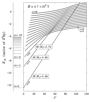
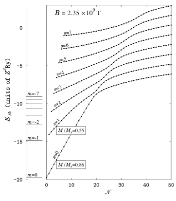
Figure 1: Energy levels and parameters of the bound-ion cyclotron transitions for He⁺ in the magnetic field of $4.7\times 10^{8}$ T (top) and $2.35\times 10^{9}$ T (bottom). In the left plots dots show the energies of the tightly-bound states for different values of the quantum number ${\mathcal{N}}$. Smooth solid lines connect the energies for visualization of the $s$-branches, and the ratios $M/M_{s}$ are deduced from the linear parts of the branches. The energies for an infinitely heavy ion are shown by the horizontal bars labeled by the magnetic quantum number $m$. Right plots show the parameters $C_{1}$ and $C_{2}$ (see Eq. (36)) for the bound-ion cyclotron absorption transitions along the computed $s$-branches of states.

The properties of He⁺ for the magnetic field strength of $4.7\times 10^{8}$ T (the corresponding value in atomic units is $B=2000$) are demonstrated in the top plots of Fig. 1. The discrete energies of the ion shown by dots group into the $s$-branches shown by smooth solid lines. For an infinitely heavy ion, the branches merge to the internal electron energies $\varepsilon_{s}$ shown by horizontal bars and labeled by the values of the conventional magnetic quantum number $m=-s$, cf. the relation (35). These energies have been addressed both analytically and numerically in many previous studies (see, e.g., Ref. Ruder_1994 and the references therein) and are reproduced in our calculations by setting $1/M=0$.

The property important for identifying the bound-ion cyclotron transitions are linear-like dependencies of the energies $E_{{\mathcal{N}}{s}}$ on ${\mathcal{N}}$. The numerically calculated energies depend on ${\mathcal{N}}$ almost linearly for the entire $s=0$ branch. At higher $s$, the growth of $E_{{\mathcal{N}}{s}}$ with ${\mathcal{N}}$ is close to linear only for low-lying energies, ${\mathcal{N}}=s,s+1,s+2,\ldots$. The linear parts of the energy branches correspond to the perturbation regime, considered in Sec. III.B. By fitting these parts by the formula (28), the ratios $M/M_{s}$ are estimated and indicated in the plot. The values for the ratios are lower for higher $s$-branches: $0.96$, $0.85$ and $0.72$ for $s=0$, $1$ and $2$, respectively. Thus, the ion’s effective masses increase with increasing the internal excitations.

At ${\mathcal{N}}\to\infty$ the couplings between the channels vanish, and the quantum states converge to the states computed within a single-channel (adiabatic) approximation. The ion energies approach the values that are multiples of the nucleus cyclotron energy $\Omega_{0}=ZB/M_{0}$, where $M_{0}$ is the nucleus mass. These thresholds correspond to the detached electron and nucleus, with the electron occupying the ground Landau level and the nucleus occupying the ground as well as the excited levels.

At intermediate values of ${\mathcal{N}}$, the neighboring branches approach each other. To visualize the branches of the discrete energy levels in the domains of nearest approach, the levels can be connected by lines which either cross or avoid the crossings. We opted to show the line $s=0$ as crossing the other lines, and the lines $s=1,2,\ldots$ as exhibiting avoided crossings. Thus, with increasing ${\mathcal{N}}$, the energies $E_{{\mathcal{N}}{s}}$ increase infinitely for $s=0$ and approach the thresholds $(s-1)\Omega_{0}$ for $s=1,2,\ldots$.

Notice that the states with $E_{{\mathcal{N}}{s}}>0$ belong to the continuum. Neglecting the coupling of the c.m. to the internal motions, the positive-energy states are computed as bound, whereas in reality they are quasi-bound (auto-ionizing) states because of the coupling. All the branches shown in Fig. 1 have the minimum-energy ${\mathcal{N}}=s$ states below the continuum $E=0$. The set of such branches for $B=4.7\times 10^{8}$ T is restricted to $s=0,1,\ldots,16$. Higher branches comprise the quasi-bound states only, and we do not include them in the figure.

As Fig. 1 shows, the levels with ${\mathcal{N}}=s$ for the bound moving He⁺ are shifted towards the continuum edge with respect to the levels with $m=-s$ for the infinitely heavy ion. This implies that already the lowest states in the moving ion are bound weaker than the states with the similar electronic excitations in the infinitely heavy ion. The only exception is the lowest state ${\mathcal{N}}=s=0$, whose binding energy is not affected by the c.m. motion. The energy offsets increase with increasing $s$ resulting in the finite number of branches below the continuum edge.

According to the general considerations presented above, the bound-ion cyclotron transitions are the transitions between the neighboring states within the computed branches. These transitions satisfy the selection rules (26). The branch numbers $s$ can be regarded as enumerating the internal excitations. For the nearly linear parts of the branches, the internal excitations correspond to the same effective masses $M_{s}$ deduced by fitting the energies by the perturbation dependence (28). For the non-linear parts around and beyond the avoided crossings the ion states still can be considered as states of similar “internal nature”, based on the symmetry and “smoothness” of the lines connecting the discrete energy values.

The transition energies and oscillator strengths for the bound-ion cyclotron transitions are computed according to Eqs. (90). To quantify the deviations of the numerical results both from the results for the reference bare ion and from the perturbation results (30), we have calculated and plotted in Fig. 1 the parameters

$$C_{1} = \omega_{{\mathcal{N}}^{\prime}\!,\,{\mathcal{N}}}/\omega^{\rm cyc}_{N^{\prime}\!,N}~{},$$

$$C_{2} = \left(f_{{\mathcal{N}}^{\prime}\!,\,{\mathcal{N}}}/f^{\rm cyc}_{N^{\prime}\!,N}\right)\left(\omega^{\rm cyc}_{N^{\prime}\!,N}/\omega_{{\mathcal{N}}^{\prime}\!,\,{\mathcal{N}}}\right)^{3}~{}.$$ (36)

For the bare ion, we have $C_{1}=C_{2}=1$. Within the perturbation regime for the coupling between c.m. and internal motions, we expect $C_{1}=M/M_{s}<1$ and $C_{2}=1$.

For $B=4.7\times 10^{8}$ T, in close relation to the properties of the ion energies, the parameters $C_{1}$ and $C_{2}$ show the perturbation regime to hold for the bound-ion cyclotron transitions along the entire $s=0$ branch as well as for the transitions involving the states up to ${\mathcal{N}}\approx 45$ along the $s=1$ branch. For higher internal excitations, $C_{1}$ and $C_{2}$ deviate from constant values and depend on the quantum number ${\mathcal{N}}$, which reflects the effects of the internal structure on the cyclotron transitions of the entire ion. For $s>1$, these effects are already prominent starting from the lowest transition states ${\mathcal{N}}=s$.

Similar properties of the levels and bound-ion cyclotron transitions are displayed by He⁺ in a higher magnetic field of $2.35\times 10^{9}$ T ($B=10\,000$ in atomic units). The results of numerical calculations are presented in the bottom plots of Fig. 1. We have restricted the computations to the branches that are below the continuum at ${\mathcal{N}}=s$. The number of these branches, $s=0,1,\ldots,7$, is smaller than the number of branches studied for the lower magnetic field strength. The branches are well separated from each other, including the domains of avoided crossings. Therefore, we have selected the $s=0$ branch as undergoing the avoided crossing and approaching the continuum threshold $E=0$ at ${\mathcal{N}}\to\infty$, in contrast to the $s=0$ branch in the top plot of the figure. For higher magnetic fields, the perturbation treatment of the coupling of the c.m. to the electronic motion becomes progressively less accurate. The numerical multi-channel calculations show that the ion properties can be described in terms of effective masses for only a small portion of the quantum states: ${\mathcal{N}}\lesssim 15$ for the $s=0$ branch and a few lowest states for the $s=1$ branch. The corresponding ratios of the mass of the ion to the effective masses are $0.86$ and $0.55$, respectively. For higher $s$-branches, the effects of the internal structure on the bound-ion cyclotron transitions are essentially non-perturbative.

V.2 Negative ions: atomic and cluster magnetically-induced anions

As the magnetically-induced anions is a rather unconventional type of ions, it is worthwhile to outline their binding mechanism and properties before discussing the bound-ion cyclotron transitions. The origin of the binding is a combination of the long-range electron correlation in the anion and the confining magnetic field. At large distances $r$ from the neutral core to the excess electron the correlation results in a local polarization potential with a “strength” determined by the polarizability $\kappa$ of the core.

In the absence of magnetic field, the correlation and emerging long-range potential play a primary role, with respect to the role of non-local short-range interaction, in forming the so-called correlation-bound anions Sommerfeld_2010 . An external magnetic field adds a lot to stability of the anionic states and makes the long-range binding possible when the polarization potential is too weak to support a stable anion without the field. In addition, the presence of a magnetic field enables a long-range binding in a sequence of excited anionic states. The magnetically-induced anionic states thus emerge as the states formed exclusively in the magnetic field.

For infinitely heavy anions, the sequence of the magnetically-induced anionic states was formally predicted to be infinite AHS_1981 . The states are characterized by the quantized values (16) of the longitudinal angular momentum of the attached electron. The corresponding electronic energies $\varepsilon_{s}$ have been explicitly estimated in Ref. BSC2000 :

$$\varepsilon_{0} =-0.31\kappa^{2}B^{2}~{}, s =0~{},$$ (37)

$$\varepsilon_{s} =-0.12\kappa^{2}B^{3}\lambda_{s}^{2}~{}, s =1,2,\ldots~{},$$ (38)

where $\lambda_{1}=1$, $\lambda_{s}=[1-(1.5/s)]\lambda_{s-1}$ for $s\geq 2$, and the atomic units are used for the energies, polarizability and the magnetic field strength. These estimates apply to small field strengths, $B\ll 1$. The energies $\varepsilon_{s}$ do not include the zero-point Landau energy for the electron, so that $|\varepsilon_{s}|=-\varepsilon_{s}$ are the binding energies. Different scaling of the energies with the the field strengths for the ground $s=0$ and excited $s>0$ states results from different localization of the excess electron in the plane transverse to the field. For $s=0$ the electron density is maximal at the location of neutral system, whereas for $s>0$ the maximum of the density is shifted away from the system. As a result, $\varepsilon_{0}$ is sensitive to a divergent behavior of the polarization potential at the origin, and the numerical prefactor in Eq. (37) is model-dependent. For details, we refer to the studies BSC-review ; BSC2007 . In contrast, the energies of excited states are not sensitive to the core of polarization potential in the presence of the field. It has also been recognized BSC-review ; Dubin that the $s=0$ state manifests itself only for systems which do not form stable anions without magnetic field. The sequence $s=1,2,\ldots$ of excited states emerges therefore on top of the ground magnetically-induced $s=0$ state or of the conventional anionic state perturbed by the magnetic field.

With account for the c.m. degrees of freedom, the energies $E_{{\mathcal{N}}{s}}$ of the magnetically-induced states are specified, in addition to $s$, by the quantum number ${\mathcal{N}}$. The coupling between the electronic and c.m. motions destroys the states with high $s$, and the sequence of magnetically-induced states turns out to be finite BSC-review . Depending on systems and on magnetic field strength, there can be a few $s$-branches of the bound states, a single branch or even a single state or no bound states at all.

Table 1: The cyclotron energies $\Omega$ of the bare ions, the energies $\varepsilon_{s}$ of the infinitely heavy anions, and the parameters of magnetically-induced energy branches $E_{{\mathcal{N}}{s}}$ of moving anions (see Eq. (39)) at the magnetic field strengths of $50$ T. The number $s$ numerates the branches of bound states, $E_{{\mathcal{N}}{s}}<0$, for the moving anions. The numbers of branches are finite and restricted to those studied in the table.

ion	$\Omega$ (MHz)		$\;s\;$	$-\varepsilon_{s}$ (MHz)		$-E_{-s,s}$ (MHz) a)		$\Omega_{s}$ (MHz) a)		$M/M_{s}$ a)		$M/M_{s}$ b)
Xe-	5.	800	0	7.	135$\times 10^{4}$	7.	134$\times 10^{4}$	5.	800	1.		1.
Xe${}_{4}^{-}$	1.	447	0	1.	142$\times 10^{6}$	1.	142$\times 10^{6}$	1.	447	1.		1.
			1	94.	02	91.	17	1.	402	0.	9685	0.	9796
			2	5.	876	2.	452	0.	5046	0.	3486	0.	4918
Xe${}_{13}^{-}$	0.	4462	1	993.	1	992.	2	0.	4458	0.	9991	0.	9994
			2	62.	07	60.	74	0.	4338	0.	9722	0.	9755
			3	15.	52	13.	81	0.	3800	0.	8516	0.	8618
			4	6.	062	4.	084	0.	2597	0.	5820	0.	6207
			5	2.	970	0.	9017	0.	09799	0.	2196	0.	3461
Ar-	19.	06	0	1.	130$\times 10^{4}$	1.	128$\times 10^{4}$	19.	04	0.	9987	1.
Ar${}_{4}^{-}$	4.	765	0	1.	808$\times 10^{5}$	1.	808$\times 10^{5}$	4.	765	1.		1.
			1	14.	893	7.	293	2.	272	0.	4767	0.	7401
Ar${}_{13}^{-}$	1.	466	1	157.	3	154.	4	1.	438	0.	9808	0.	9875
			2	9.	831	6.	060	0.	8001	0.	5456	0.	6331
a) coupled-channel calculations
b) perturbation estimates

For magnetic field strengths achievable in laboratories, the conventional anionic states, if exist, are not much influenced by the field. There, the coupling between the excess electron and c.m. motion has only a minor if not negligible impact on the ion motion and radiative transitions. The examples considered below display the same properties for the ground magnetically-induced states. In contrast, for the exited states bound due to the field, the coupling significantly affects the internal and collective motions, and the bound-ion cyclotron transitions differ from those of the reference bare ions.

For the numerical studies, we have selected the noble gas atoms Xe and Ar and their small clusters at a large magnetic field strength $B=50$ T which can be approached with resistive magnets in advanced experimental setups lab1 ; lab2 . The calculations utilize the polarizability values $27.815$ a.u. for Xe and $11.07$ a.u. for Ar provided in the dipole polarizability tables dp-tables according to the experimental measurements.

The closed-shell Xe and Ar do not form conventional stable anions, and thus they can display the ground magnetically-bound anionic states. The clusters of these atoms can form anions in the absence of magnetic field, due to increasing polarization attraction of the excess electron with increasing number of the atoms in clusters. However, a minimum number of cluster atoms required to attach the electron is known reliably only for the Xe clusters studied by an ab initio Green functions method Xe_clusters and found to form stable correlation-bound anions starting from a size of five atoms. To address the magnetically-induced states with $s=0$, we have performed computations for Xe${}_{4}^{-}$, which is the largest Xe cluster anion possessing this branch of states. To study the effect of cluster size on the energies and transitions for the $s>0$ states, we have performed computations for Xe${}_{13}^{-}$ formed by a smallest magic number of cluster atoms. For Ar, we have considered the magnetically-induced anions with the same numbers of cluster atoms, $4$ and $13$, as for Xe. Since the polarizability of Ar is smaller than that of Xe, a minimum number of atoms in a stable conventional Ar cluster anion is larger than five. Therefore, Ar${}_{4}^{-}$ is not stable in the absence of magnetic field, and it can display the $s=0$ magnetically-induced states. For Ar${}_{13}^{-}$, we did not address the $s=0$ states, for an analogy of the consideration with that for Xe${}_{13}^{-}$.

To compute the magnetically-induced cluster anions, we employ the same frameworks of perturbation and coupled-channel approaches as for the atomic ions. Since the excess electron resides on a diffuse orbital extending far away from the cluster cores, to a good approximation the clusters can be considered as entities characterized by masses and polarizabilities. The cluster polarizabilities are evaluated as the multiples of atomic polarizabilities and the numbers of the cluster atoms. To justify the latter approximation, we refer to ab initio studies Xe_dimer of the polarizability of Xe dimer. It was found that though the polarizability of the dimer is anisotropic and deviates from the sum of atomic polarizabilities, this does not influence significantly the binding energies of the anionic states induced by a magnetic field aligned along the dimer axis. The structures of clusters formed by $4$ and $13$ atoms (a regular tetrahedron and a regular icosahedron with an extra atom at the center, respectively) have higher symmetries, and we may expect even a less pronounced, than for the dimer, impact of a non-additivity and anisotropy of the cluster polarizabilities on the magnetically-bound anionic states.

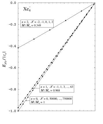
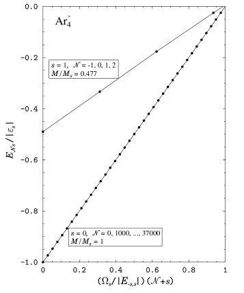
Figure 2: Energy levels and parameters of the bound-ion cyclotron transitions of the magnetically-induced Xe${}_{4}^{-}$ (top) and Ar${}_{4}^{-}$ (bottom) in a magnetic field of $50$ T. The left plots show the $s$-branches of bound levels, with dots displaying the discrete levels with the numbers ${\mathcal{N}}$ as indicated. The values $M/M_{s}$ are determined by approximating the energies by linear dependencies on ${\mathcal{N}}$. The right plots show the parameters $C_{1}$ and $C_{2}$ of the bound-ion absorption cyclotron transitions ${\mathcal{N}}\to{\mathcal{N}}+1$ along the branches of the computed levels. For Xe${}_{4}^{-}$, $C_{2}=1$ for both $s=0$ and $s=1$ as shown by the solid line.

For the anions considered, the coupled-channel calculations yield the energy levels which follow fairly well a linear dependence on ${\mathcal{N}}$,

$$E_{{\mathcal{N}}{s}}=E_{-s,s}+\Omega_{s}({\mathcal{N}}+s)~{}.$$ (39)

This allows one to deduce an effective mass $M_{s}$ of the ion from the slope $\Omega_{s}$ which has a meaning of the effective cyclotron energy of anion. In Table 1 we indicate the values of the minimum energy $E_{-s,s}$, the slope $\Omega_{s}$ and the ratio $M/M_{s}$ for the $s$-branches computed. We also include the cyclotron energies $\Omega$ of the bare ions, the energies $\varepsilon_{s}$ of the infinitely heavy anions, and the ratios $M/M_{s}$ determined according to the perturbation formula (69).

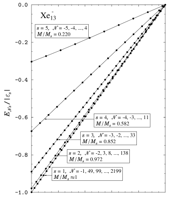
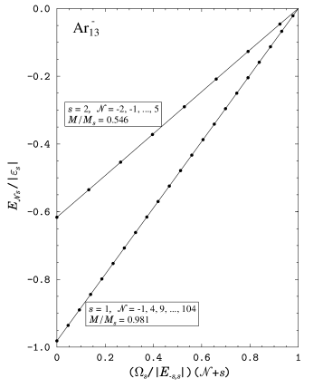
Figure 3: Same as in Fig. 2 but for Xe${}_{13}^{-}$ and Ar${}_{13}^{-}$. For Xe${}_{13}^{-}$, $C_{2}=1$ for both $s=1$ and $s=2$.

The atomic anions Xe^- and Ar^- display only the $s=0$ branches of the magnetically-induced states, whereas the higher $s$-branches are entirely destroyed by the coupling between the motions of c.m. and excess electron. The numbers of the bound states with different ${\mathcal{N}}$ values are equal to the ratios $-E_{-s,s}/\Omega_{s}$ and are very large in the $s=0$ branches, about $12\,300$ for Xe^- and about $600$ for Ar^-. The anions move essentially as the bare ions ($M/M_{s}=1$) as found from both the coupled-channel and perturbation treatments. Consequently, the parameters of the bound-ion cyclotron transitions are $C_{1}=C_{2}=1$, i.e. the transition energies and the oscillator strengths are the same as for the reference bare ions.

The magnetically-induced anions of Xe and Ar clusters display higher $s$-branches of states as well as cyclotron transitions deviating from those of the reference bare ions. The results are presented in Figs. 2 and 3. The left plots in the figures show the energies for the anions bound in different states of the quantized collective motion. The zero-point Landau energy for the excess electron has been subtracted from the computed energies, and the zero energy value in the plots corresponds to the detachment threshold. The energies $E_{{\mathcal{N}}{s}}$ for the moving anions are scaled by the binding energies $|\varepsilon_{s}|$ for the infinitely heavy anions and shown as functions of $(\Omega_{s}/|E_{-s,s}|)({\mathcal{N}}+s)$, where $E_{-s,s}$ is the minimum energy value in the sequence $E_{{\mathcal{N}}{s}}$ with ${\mathcal{N}}=-s,-s+1,\ldots$, and $\Omega_{s}$ is the effective cyclotron energy determined from the linear growth of the energies with ${\mathcal{N}}$. The scaling is convenient for presenting the results for anionic states with significantly different energy values (see Table 1). The right plots in Figs. 2 and 3 show the parameters $C_{1}$ and $C_{2}$ for the bound-ion cyclotron transitions along the branches of levels.

Figs. 2 and 3 clearly display a linear increase of quantum energies with ${\mathcal{N}}$ increasing along the $s$-branches. The anion’s motion in the magnetic field is therefore described fairly well in terms of the effective masses indicated in Table 1 and in the figures. The branches terminate when approaching, with increasing ${\mathcal{N}}$, the detachment threshold $E=0$. Above the threshold, the branches would include the positive energies of auto-detaching states calculating which goes beyond the scope of this paper.

With increasing number $N_{\rm at}$ of cluster atoms, the numbers of states with different ${\mathcal{N}}$ in a branch increase as $-E_{-s,s}/\Omega_{s}\sim-\varepsilon_{s}/\Omega\propto N_{\rm at}^{3}$, since $-\varepsilon_{s}\propto\kappa^{2}\propto N_{\rm at}^{2}$, and $\Omega\propto N_{\rm at}^{-1}$ due to increasing with $N_{\rm at}$ polarizabilities and masses of the clusters. The $s=0$ branches for the cluster anions of four atoms comprise the numbers of states exceeding those for the atomic anions by a factor of $64$, as reflected in Fig. 2 by the numbers of states $\approx 750\,000$ for Xe${}_{4}^{-}$ and $\approx 37\,000$ for Ar${}_{4}^{-}$. These numbers are very large, and the discrete energies in the branches are shown with the increments of $50\,000$ and $1\,000$, respectively, in varying ${\mathcal{N}}$. The numerical calculations for the $s=0$ branches yield the effective masses coinciding with the masses of anions, and the values $C_{1}=C_{2}=1$ for the parameters of the cyclotron transitions. As expected from the property of the atomic anions, the quantum levels and cyclotron transitions of the cluster anions for the $s=0$ branches are not influenced by the coupling between the motions of c.m. and excess electron.

In contrast to the atoms, the clusters considered in Fig. 2 do possess higher $s$-branches of the magnetically-induced anionic states. In addition to the $s=0$ branches, the calculations reveal bound states forming the $s=1$ and $s=2$ branches for Xe${}_{4}^{-}$, and the $s=1$ branch for Ar${}_{4}^{-}$. The effective mass exceeds the total mass only slightly for the $s=1$ states of Xe${}_{4}^{-}$ but quite substantially for the $s=2$ states of Xe${}_{4}^{-}$ and for the $s=1$ states of Ar${}_{4}^{-}$. The values of $C_{1}$ coincide fairly well with the mass ratios $M/M_{s}$, and the values for $C_{2}$ do not significantly deviate from unity (for the transitions along the $s=1$ branch of levels of Xe${}_{4}^{-}$, the calculations yield $C_{2}=1$ with a high accuracy). Thus, the effect of internal structure on the bound-ion cyclotron transitions follows well the perturbation regime.

The larger cluster anions addressed in Fig. 3 display more magnetically-induced states. For Xe${}_{13}^{-}$, the states group in more branches, $s=1,\ldots,5$, than for Xe${}_{4}^{-}$. For Ar${}_{13}^{-}$, we encounter the same two branches, $s=1,2$, as for Ar${}_{4}^{-}$, which comprise more levels with different ${\mathcal{N}}$. The effective Xe${}_{13}^{-}$ mass for $s=1$ coincides with the total mass, and the anion moves in the field essentially as a bare ion. Consequently, the bound-ion cyclotron transitions are not affected by the coupling between the motions of c.m. and excess electron ($C_{1}=C_{2}=1$). The branches $s=2$ of Xe${}_{13}^{-}$ and $s=1$ of Ar${}_{13}^{-}$ correspond to the effective masses only slightly exceeding the total masses, and the cyclotron transitions of anions in these internal configurations are only slightly influenced by the coupling. For the $s=2$ branch of Xe${}_{13}^{-}$, $C_{2}=1$ with a high accuracy implying an excellent agreement between the perturbation and coupled-channel results. For higher $s$ for Xe${}_{13}^{-}$ as well as for $s=2$ for Ar${}_{13}^{-}$, the $C_{2}$ values deviate from unity and slightly increase with increasing ${\mathcal{N}}$. This implies that the perturbation approach becomes progressively less accurate for higher internal excitations.

Overall, the numerical studies demonstrate that the impact of the internal structure on the bound-ion cyclotron transitions is guided by the ratio of the binding energy of the infinitely heavy ion and the cyclotron energy of the reference bare ion. The smaller this ratio is, the more significant are the deviations of the quantized motion of ion as a whole and the related cyclotron transitions from those of the bare ion. For the magnetically-induced anions considered, these deviations, when emerge, follow well a perturbation regime described in terms of the effective masses.

VI Conclusions

We have derived a theoretical framework for quantum description of the motion and radiative transitions for ions with internal structure in external magnetic fields. We have focused on the collective motion and the related cyclotron-type radiative transitions for the entire ions. These bound-ion cyclotron transitions are primarily associated with the properties of the quantum motion of the ions as a whole in the field. The coupling of the internal structure of the ions to the collective motion in the field makes the transitions to differ from the cyclotron transitions for the bare ions with the same masses and charges. The developed theoretical description utilizes the integrals of motion for the ions. A general perturbation approach to the coupling for the atomic ions is facilitated by the conservation of the longitudinal angular momentum for the isolated electronic configuration. The bound-ion cyclotron transitions have been identified by specific selection rules. The perturbation approach quantifies the transition energies and oscillator strengths for the bound-ion cyclotron transitions in terms of the effective masses for the ions. Analytical results have been augmented by the results of numerical coupled-channel calculations of the ion states and radiative transitions.

We have studied the bound-ion cyclotron transitions for both positive and negative complex ions. Numerical results have been obtained for the He⁺ ion in strong magnetic fields typical for neutron stars, and for the negative magnetically-bound atomic and cluster ions for the field strengths typical for laboratory experiments. The calculations reveal significant effects of the internal structure on the cyclotron transitions of the entire ions. For the He⁺ ions, the presented theoretical studies could be used for interpretations of the spectral observations of neutron stars with strong magnetic fields. The negative magnetically-induced ions are yet to be directly probed in an experiment on magnetically-guided electron attachment. In particular, experimental detection of the bound-ion cyclotron transitions would signify the magnetically-induced binding of the excess electron by a neutral complex.

Appendix A The Landau states

The quantum states for the Hamiltonian (2) are the common eigenstates of the operators ${\mathit{\Pi}}_{\perp}^{2}={\mathit{\Pi}}_{x}^{2}+{\mathit{\Pi}}_{y}^{2}$, $K_{\perp}^{2}=K_{x}^{2}+K_{y}^{2}$, and $L_{z}$, where

$$({\mathit{\Pi}}_{x},{\mathit{\Pi}}_{y},0) =\mathbf{P}_{\perp}-(Q/2)\mathbf{B}\times\mathbf{R}_{\perp}~{},$$ (40)

$$(K_{x},K_{y},0) =\mathbf{P}_{\perp}+(Q/2)\mathbf{B}\times\mathbf{R}_{\perp}~{},$$ (41)

$$(0,0,L_{z}) =\mathbf{R}_{\perp}\times\mathbf{P}_{\perp}$$ (42)

are the kinetic, pseudo, and angular momenta, respectively, for the motion of a particle with charge $Q$ in the plane perpendicular to the magnetic field. Their eigenvalues are determined by the integers:

$${\mathit{\Pi}}_{\perp}^{2} =|Q|B(2N+1)~{}, N =0,1,2,\ldots~{},$$ (43)

$$K_{\perp}^{2} =|Q|B(2N_{0}+1)~{}, N_{0} =0,1,2,\ldots~{},$$ (44)

$$L_{z} =-\sigma L~{}, L =0,\pm 1,\pm 2,\ldots~{},$$ (45)

where $\sigma$ is the sign of $Q$.

The operator ${\mathit{\Pi}}_{\perp}^{2}$ determines the kinetic energy of the particle given by the Hamiltonian (2), whereas the operators $K_{\perp}^{2}$ and $L_{z}$ are the integrals of motion for this Hamiltonian. In particular, $K_{\perp}^{2}$ relates to the guiding center of the particle’s rotation around the field lines, see, e.g., AHS_1981 . The eigenvalues (43) yield the energies (3) for the Landau states, which are degenerate with respect to the numbers $N_{0}$ and $L$.

Only two of the three numbers $N$, $N_{0}$ and $L$ are independent, and the relation $N=N_{0}+L$ (see Eq. (4)) holds, as a result of the operator relation

$${\mathit{\Pi}}_{\perp}^{2}=K_{\perp}^{2}-2QBL_{z}~{}.$$ (46)

Thus, any pair from the set $N$, $N_{0}$ and $L$ can be used to designate the eigenstates of the Hamiltonian (2). In our considerations, we use the pair $N$, $N_{0}$.

For a particle with charge $Q$ occupying a Landau state with the quantum numbers $N$ and $N_{0}$, the normalized wave function in ${\bf R}_{\perp}=(X,Y)$ is

$${\mathit{\Phi}}^{(Q)}_{N,N_{0}}({\bf R}_{\perp})=\frac{e^{{\rm i}{\sigma}(N_{0}-N)\varphi}}{\sqrt{2\pi}\lambda_{Q}}\,F_{N,N_{0}}(u),$$ (47)

where $\varphi=\tan^{-1}(Y/X)$, $u=(X^{2}+Y^{2})/(2\lambda_{Q}^{2})$, and $\lambda_{Q}=(|Q|B)^{-1/2}$. The functions $F_{N,N_{0}}$ are equal to zero if $N<0$ or $N_{0}<0$, while for non-negative indices they are given by the expression

$$F_{N,N_{0}}(u) = (-1)^{N-N_{0}}F_{N_{0},N}(u)$$ (48)

$$= \left(\frac{N!}{N_{0}!}u^{N_{0}-N}{\rm e}^{-u}\right)^{1/2}L_{N}^{N_{0}-N}(u),$$

where $L_{N}^{s}(u)$ are the Laguerre polynomials. The set of Landau functions (47) with $N=0,1,2,\ldots$, $N_{0}=0,1,2,\ldots$ possesses the standard properties of orthogonality and completeness. The relations

$$({\mathit{\Pi}}_{x}-{\rm i}\,\sigma{\mathit{\Pi}}_{y}){\mathit{\Phi}}^{(Q)}_{N,N_{0}} =-{\rm i}\,p_{Q}\sqrt{N+1}\,{\mathit{\Phi}}^{(Q)}_{N+1,N_{0}},$$

$$({\mathit{\Pi}}_{x}+{\rm i}\,\sigma{\mathit{\Pi}}_{y}){\mathit{\Phi}}^{(Q)}_{N,N_{0}} =\;\;\;{\rm i}\,p_{Q}\sqrt{N}\,{\mathit{\Phi}}^{(Q)}_{N-1,N_{0}},$$

$$(K_{x}-{\rm i}\,\sigma K_{y}){\mathit{\Phi}}^{(Q)}_{N,N_{0}} =-{\rm i}\,p_{Q}\sqrt{N_{0}}\,{\mathit{\Phi}}^{(Q)}_{N,N_{0}-1},$$

$$(K_{x}+{\rm i}\,\sigma K_{y}){\mathit{\Phi}}^{(Q)}_{N,N_{0}} =\;\;\;{\rm i}\,p_{Q}\sqrt{N_{0}+1}\,{\mathit{\Phi}}^{(Q)}_{N,N_{0}+1},$$ (49)

where $p_{Q}=(2|Q|B)^{1/2}$, are convenient for calculating matrix elements with the Landau functions.

The cyclotron transition amplitudes are determined by the matrix elements $D^{(\beta)}_{N^{\prime},N}$ of the dipole operators (5) with the Landau functions (47). The corresponding transition energies are $\omega^{\rm cyc}_{N^{\prime},N}=E^{\rm Lan}_{N^{\prime}}(\Omega)-E^{\rm Lan}_{N}(\Omega)$, and the oscillator strengths are

$$f^{\rm cyc}_{N^{\prime},N}=2\,\omega^{\rm cyc}_{N^{\prime},N}\left|D^{(\beta)}_{N^{\prime},N}\right|^{2}~{}.$$ (50)

Direct calculations show that the non-vanishing matrix elements are

$$D^{(\beta)}_{N-\beta\sigma,N}=\langle{\mathit{\Phi}}^{(Q)}_{N-\beta\sigma,N_{0}}\left|D^{(\beta)}\right|{\mathit{\Phi}}^{(Q)}_{N,N_{0}}\rangle~{},$$ (51)

and therefore the selection rules and transition energies are given by Eqs. (6) and (7), respectively. The matrix elements (51) are readily evaluated using the relations (49). Four cases, selected by the signs of the charge $\sigma=\pm 1$ and circular polarization $\beta=\pm 1$, cast into the expression (8).

The matrix elements (51) are calculated with pairs of the Landau functions with the same quantum number $N_{0}$. Since this number does not change in the course of the cyclotron transitions, we do not include it in the indices for the dipole matrix elements. Notice that the dipole matrix elements also differ from zero when being calculated with the Landau functions with neighboring values for $N_{0}$ and the same values for $N$. They relate then to the zero transition energies and do not describe physically meaningful transitions.

Appendix B System of charges in a magnetic field: integrals of motion and selection rules

Similar to the one-particle Hamiltonian (2), the integrals of motion for the many-particle Hamiltonian (9) are determined by the operators $K_{\perp}^{2}=K_{x}^{2}+K_{y}^{2}$ and ${\cal L}_{z}$ that are now the total pseudo- and angular momenta for the motion of the system of particles in the plane perpendicular to the magnetic field,

$$(K_{x},K_{y},0) =\sum_{a}\left(\mathbf{p}_{\perp{a}}+\frac{e_{a}}{2}\,\mathbf{B}\times\mathbf{r}_{\perp{a}}\right)~{},$$ (52)

$$(0,0,{\cal L}_{z}) =\sum_{a}{\bf r}_{\perp{a}}\times{\bf p}_{\perp{a}}~{}.$$ (53)

The many-particle pseudo-momentum (52) can be transformed to the one-particle form (41) when expressed in terms of an appropriate canonical pair ${\bf R}_{\perp}$, ${\bf P}_{\perp}$. This pair can be introduced in several ways. For example, it can be related to the center of charge for the system. Another choice is to relate ${\bf R}_{\perp}$, ${\bf P}_{\perp}$ to the c.m. motion followed by a gauge transformation of the operators.

As the total pseudo-momentum can be transformed to the one-particle form, we keep the same notation for this operator as introduced for the single charge. We also keep the notation $N_{0}$ for the quantum number which determines the eigenvalues of $K_{\perp}^{2}$. The latter eigenvalues are given by Eq. (44) applicable to many-particle systems. The eigenvalues of ${\cal L}_{z}$ are integers which we specify by the relation (cf. Eq. (45))

$$\mathcal{L}_{z} =-\sigma\mathcal{L}~{}, \mathcal{L} =0,\pm 1,\pm 2,...~{}.$$ (54)

The dipole transitions for the system are determined by the operators (11). To derive the selection rules, we consider the matrix elements $\bm{\mathcal{D}}_{q^{\prime}q}$ for the dipole moment (12), where $q$ and $q^{\prime}$ denote the quantum states with the numbers $N_{0}$, $\mathcal{L}$ and $N^{\prime}_{0}$, $\mathcal{L}^{\prime}$, respectively.

The eigenvalues (44) and (54) allow one to relate $\bm{\mathcal{D}}_{q^{\prime}q}$ to the matrix elements of the commutators,

$$p_{Q}^{2}\left(N^{\prime}_{0}-N_{0}\right)\bm{\mathcal{D}}_{q^{\prime}q} = \left[K_{\perp}^{2},\bm{\mathcal{D}}\right]_{q^{\prime}q}~{},$$ (55)

$$-\sigma\left(\mathcal{L}^{\prime}-\mathcal{L}\right)\bm{\mathcal{D}}_{q^{\prime}q} = \left[\mathcal{L}_{z},\bm{\mathcal{D}}\right]_{q^{\prime}q}~{}.$$ (56)

By evaluating the commutators of the Hamiltonian (9) with the radius $\mathbf{r}_{a}$, one obtains the relation

$$\left(E_{q^{\prime}}-E_{q}\right)\bm{\mathcal{D}}_{q^{\prime}q}={\rm i}\,\bm{\mathcal{J}}_{q^{\prime}q}~{},$$ (57)

where $E_{q^{\prime}}$ and $E_{q}$ are the state energies and $\bm{\mathcal{J}}_{q^{\prime}q}$ are the matrix elements for the current

$$\bm{\mathcal{J}}=\sum_{a}\frac{e_{a}}{m_{a}}\left(\mathbf{p}_{a}-\frac{e_{a}}{2}\,\mathbf{B}\times\mathbf{r}_{a}\right)~{}.$$ (58)

To derive the selection rules for the numbers $N^{\prime}_{0}$ and $N_{0}$, we use Eq. (57) to transform the relation (55) as follows

$$p_{Q}^{2}\left(N^{\prime}_{0}-N_{0}\right)\left(E_{q^{\prime}}-E_{q}\right)\bm{\mathcal{D}}_{q^{\prime}q}={\rm i}\,\left[K_{\perp}^{2},\bm{\mathcal{J}}\right]_{q^{\prime}q}~{}.$$ (59)

It is straightforward to prove that the current commutes with $K_{\perp}^{2}$ and therefore

$$\left(N^{\prime}_{0}-N_{0}\right)\left(E_{q^{\prime}}-E_{q}\right)\bm{\mathcal{D}}_{q^{\prime}q}=0~{}.$$ (60)

For the physically meaningful transitions, the state energies are different, $E_{q^{\prime}}\neq E_{q}$. Therefore, the transitions with $\bm{\mathcal{D}}_{q^{\prime}q}\neq 0$ correspond to the selection rule

$$N^{\prime}_{0}=N_{0}~{}.$$ (61)

Notice that this general selection rule holds for an arbitrary polarization of radiation, i.e. for the transitions determined not only by the cyclic components (11) but by projection of the dipole operator on an arbitrary polarization vector. On physical grounds, the number $N_{0}$ relates to the “center of quantization” in uniform space. Therefore, a change in $N_{0}$ implies the change of the reference frame, not affecting the properties of the quantum states.

To derive the selection rules with respect to the numbers $\mathcal{L}^{\prime}$ and $\mathcal{L}$, we consider the relations (56) for the cyclic components of the dipole operator,

$$\left(\mathcal{L}^{\prime}-\mathcal{L}\right)\mathcal{D}^{(\beta)}_{q^{\prime}q}=-\sigma\left[\mathcal{L}_{z},\mathcal{D}^{(\beta)}\right]_{q^{\prime}q}~{},$$ (62)

and use the commutator relations

$$[\mathcal{L}_{z},\mathcal{D}^{(\beta)}]=\beta\,\mathcal{D}^{(\beta)}$$ (63)

which are easily proved by direct calculations. Then, Eqs. (62) and (63) yield the relation

$$\left(\mathcal{L}^{\prime}-\mathcal{L}+\beta\sigma\right)\mathcal{D}_{q^{\prime}q}^{(\beta)}=0~{}.$$ (64)

Therefore, the selection rules for the transitions with $\mathcal{D}_{q^{\prime}q}^{(\beta)}\neq 0$ are

$$\mathcal{L}^{\prime}=\mathcal{L}-\beta\sigma~{}.$$ (65)

As the quantum number $N_{0}$ does not change in the course of transitions, the same selection rule, ${\mathcal{N}}^{\prime}={\mathcal{N}}-\beta\sigma$, Eq. (13), holds for the numbers ${\cal N}^{\prime}$ and ${\cal N}$.

Appendix C Perturbation treatment of the coupling between c.m. and electronic motions

When employing standard perturbation techniques to treat the coupling term $H_{3}$ in the Hamiltonian (14), we implement the integrals of motion $K_{\perp}^{2}$ and $\mathcal{L}_{z}$ already for the zero-order approximation (which is possible since the operators $K_{\perp}^{2}$ and $\mathcal{L}_{z}$ commute with the terms $H_{1}$ and $H_{2}$). The perturbation-corrected ion states emerge then as the eigenstates of the integrals of motion as well.

The zero-order approximation to the Hamiltonian (14) is the sum $H_{1}+H_{2}$, the corresponding wave functions are the products

$$\psi^{(0)}_{NN_{0}s\nu}\left(\mathbf{R}_{\perp},\left\{\mathbf{r}_{i}\right\}\right)={\mathit{\Phi}}^{(Q)}_{N,N_{0}}\left(\mathbf{R}_{\perp}\right)\phi_{s\nu}\left(\left\{\mathbf{r}_{i}\right\}\right)$$ (66)

of the eigenfunctions of the terms $H_{1}$ and $H_{2}$, and the ion energies are the sums (20) of the c.m. and electronic energies. As the canonically transformed total pseudo-momentum is the one-particle operator (41) for the c.m. motion, the c.m. Landau functions ${\mathit{\Phi}}^{(Q)}_{N,N_{0}}$ and hence the zero-order wave functions (66) are the eigenfunctions of $K_{\perp}^{2}$. The corresponding quantum number $N_{0}$ is explicitly included in the set of the numbers that label the zero-order states. Since the electronic wave functions $\phi_{s\nu}(\{{\bf r}_{i}\})$ are the eigenfunctions of $l_{z}$ with the eigenvalues $-s$, the zero-order wave functions are the eigenfunctions of $\mathcal{L}_{z}$ with the eigenvalues $-\sigma(N-N_{0})-s$ (cf. Eqs. (45), (4) and (21)). Thus, to ascribe the conserved values $-\sigma\mathcal{L}$ (see Eq. (54)) of the total longitudinal angular momentum to the zero-order states, the relation $N=N_{0}+\mathcal{L}-\sigma{s}$ is required, which yields $N={\mathcal{N}}-\sigma{s}$ (cf. Eq. (22)). Notice that the zero-order wave functions depend on the sum ${\mathcal{N}}=N_{0}+\mathcal{L}$ (cf. Eq. (10)) providing thereby the same property for the perturbation-corrected wave functions.

The perturbation corrections are determined by the matrix elements

$$\langle\psi^{(0)}_{{\mathcal{N}}{N_{0}}{s^{\prime}}\nu^{\prime}}|H_{3}|\psi^{(0)}_{{\mathcal{N}}{N_{0}}{s}\nu}\rangle=-\frac{\alpha|Q|^{1/2}B^{3/2}}{M}\,$$ (67)

$$\times\left[\sqrt{N+1}\,d^{(+\sigma)}_{s^{\prime}\nu^{\prime},s\nu}\,\delta_{s^{\prime},s-\sigma}+\sqrt{N}\,d^{(-\sigma)}_{s^{\prime}\nu^{\prime},s\nu}\,\delta_{s^{\prime},s+\sigma}\right]$$

obtained with use of the properties (49) for the c.m. Landau functions, with $d^{(\pm\sigma)}_{s^{\prime}\nu^{\prime},s\nu}=\langle\phi_{s^{\prime}\nu^{\prime}}|d^{(\pm\sigma)}|\phi_{s\nu}\rangle$ being the matrix elements of the cyclic components of electronic dipole operator ($\sigma$ is the sign of the ion’s charge). From the commutator relations $[l_{z},d^{(\pm 1)}]=\pm d^{(\pm 1)}$ it follows that non-vanishing are the elements $d^{(\pm 1)}_{s\mp{1},\nu^{\prime};s\nu}$ as reflected by the Kronecker deltas in Eq. (67).

Since the perturbation matrix elements with $s^{\prime}=s$ are equal to zero, the first-order energy corrections vanish. Standard calculations of the second-order energy corrections yield

$$E^{(2)}_{{\mathcal{N}}{s}\nu} = \frac{\alpha^{2}|Q|B^{3}}{M^{2}}\left[(N+1)G_{s\nu}^{(+)}+NG_{s\nu}^{(-)}\right],$$

$$G_{s\nu}^{(+)} = \sum_{\nu^{\prime}\neq\nu}\frac{\left|d^{(+\sigma)}_{s-\sigma,\nu^{\prime};s\nu}\right|^{2}}{\varepsilon_{s\nu}-\varepsilon_{s-\sigma,\nu^{\prime}}-\Omega}~{},$$

$$G_{s\nu}^{(-)} = \sum_{\nu^{\prime}\neq\nu}\frac{\left|d^{(-\sigma)}_{s+\sigma,\nu^{\prime};s\nu}\right|^{2}}{\varepsilon_{s\nu}-\varepsilon_{s+\sigma,\nu^{\prime}}+\Omega}~{}.$$ (68)

Similar to the zero-order energies (20), the corrections $E^{(2)}_{{\mathcal{N}}{s}\nu}$ depend linearly on $N={\mathcal{N}}-\sigma{s}$. Therefore, the sum of the zero- and second-order terms results in the oscillator-like dependence (28) of the ion energies on $N$. As a result of the coupling between c.m. and internal motions, the ion mass $M$ in the Landau energies is replaced by the effective mass $M_{s\nu}$ dependent on the internal states (cf. Eqs. (29)). In addition, the ion energies acquire the shifts $\Delta_{s\nu}$ with respect to the zero-order energies (20). The effective masses and shifts calculated from the second-order perturbation correction are

$$\frac{M}{M_{s\nu}} = 1+\frac{\alpha^{2}B^{2}}{M}\left[G_{s\nu}^{(+)}+G_{s\nu}^{(-)}\right],$$ (69)

$$\Delta_{s\nu} = \frac{\alpha^{2}|Q|B^{3}}{M^{2}}\,G_{s\nu}^{(+)}~{}.$$ (70)

It now remains to account for the perturbation corrections for the oscillator strengths. For transparency of the derivations we consider the bound-ion emission cyclotron transitions with ${\mathcal{N}}^{\prime}={\mathcal{N}}-1$ for the positive ion, $\sigma=+1$. The emitted radiation is right-polarized, $\beta=+1$. With accuracy up to the first-order perturbation corrections, the initial and final state wave-functions are

$$\psi_{{\mathcal{N}}{N_{0}}{s}\nu} = {\mathit{\Phi}}^{(Q)}_{N,N_{0}}\,\phi_{s\nu}-\sqrt{N+1}\,{\mathit{\Phi}}^{(Q)}_{N+1,N_{0}}\tilde{\phi}_{s-1,\nu}$$

$$- \sqrt{N}\,{\mathit{\Phi}}^{(Q)}_{N-1,N_{0}}\tilde{\phi}_{s+1,\nu}~{},$$

$$\psi_{{\mathcal{N}}^{\prime}{N_{0}}{s}\nu} = {\mathit{\Phi}}^{(Q)}_{N-1,N_{0}}\,\phi_{s\nu}-\sqrt{N}\,{\mathit{\Phi}}^{(Q)}_{N,N_{0}}\tilde{\phi}_{s-1,\nu}$$ (71)

$$- \sqrt{N-1}\,{\mathit{\Phi}}^{(Q)}_{N-2,N_{0}}\tilde{\phi}_{s+1,\nu}~{},$$

where $N={\mathcal{N}}-s$ (cf. Eq. (22)), and the functions

$$\tilde{\phi}_{s\pm{1},\nu}=\frac{\alpha|Q|^{1/2}B^{3/2}}{M}\,\sum_{\nu^{\prime}\neq\nu}\frac{d^{(\mp{1})}_{s\pm{1},\nu^{\prime};s\nu}\,\phi_{s\pm{1},\nu^{\prime}}}{\varepsilon_{s\nu}-\varepsilon_{s\pm{1},\nu^{\prime}}\pm\Omega}$$ (72)

include the electronic configurations admixed to the zero-order states as a result of the coupling. Due to the latter admixtures, the matrix elements of the dipole operators $\mathcal{D}^{(+1)}=D^{(+1)}+d^{(+1)}$ are contributed by the electronic transitions,

$$d^{(+1)}_{{\mathcal{N}}^{\prime},{\mathcal{N}}}=-\frac{\alpha|Q|^{1/2}B^{3/2}}{M}\,\sqrt{N}\,\left[G_{s\nu}^{(+)}+G_{s\nu}^{(-)}\right],$$ (73)

in addition to the dominant c.m. cyclotron transitions,

$$D^{(+1)}_{{\mathcal{N}}^{\prime},{\mathcal{N}}}=-\sqrt{|Q|/B}\,\sqrt{N}~{}.$$ (74)

The sums of the contributions (74) and (73) yield the total dipole elements different from the c.m. ones (74) by exactly the ratio of masses given by Eq. (69):

$$\mathcal{D}^{(+1)}_{{\mathcal{N}}^{\prime},{\mathcal{N}}}=(M/M_{s\nu})\,D^{(+1)}_{{\mathcal{N}}^{\prime},{\mathcal{N}}}~{}.$$ (75)

With account for the mass ratio factor for the transition energies $\omega_{{\mathcal{N}}^{\prime}\!,\,{\mathcal{N}}}=(M/M_{s\nu})\,\omega^{\rm cyc}_{N^{\prime}\!,N}$, we arrive at the relation $f_{{\mathcal{N}}^{\prime}\!,\,{\mathcal{N}}}=(M/M_{s\nu})^{3}f^{\rm cyc}_{N^{\prime}\!,N}$ for the oscillator strengths (see Eq. (30)).

Appendix D Coupled-channel formalism

The equations below apply to the positive hydrogen-like ions and negative magnetically-induced ions studied numerically in Section V.

D.1 Hydrogen-like ions

As the basis states for the Hamiltonian (31), we employ the Landau states of separated electron and nucleus, i.e., the states of a detached ion. The states are attributed to the quantum numbers $N_{0}$ and $\mathcal{L}$ for the integrals of collective motion B_1995 and describe the electron and nucleus occupying the Landau levels with the numbers $n_{e}$ and $n$, respectively. The corresponding energies are the sums $E^{\rm Lan}_{n_{e}}(\Omega_{e})+E^{\rm Lan}_{n}(\Omega_{0})$, where $\Omega_{e}=B$ and $\Omega_{0}=ZB/M_{0}$ are the electron and nucleus cyclotron energies, respectively ($Z$ is the nucleus charge number and $M_{0}$ is the nucleus mass). For given ${\mathcal{N}}=N_{0}+\mathcal{L}$, the Landau level numbers vary as

$$n_{e}=0,1,\ldots~{},\;\;\;n=0,1,\ldots,{\mathcal{N}}+n_{e}~{},$$ (76)

and the basis functions with the numbers $n_{e}$ and $n$ are given by the linear combinations

$$\langle{\bf R}_{\perp},{\bf r}_{\perp}|n_{e}n\rangle=$$

$$\sum_{k=-n_{e}}^{\mathcal{N}}c_{n,n_{e}+k}^{{\mathcal{N}}+n_{e}}{\mathit{\Phi}}^{(Z-1)}_{{\mathcal{N}}-k,N_{0}}({\bf R}_{\perp})\,{\mathit{\Phi}}^{(-1)}_{n_{e},n_{e}+k}({\bf r}_{\perp})$$ (77)

of the Landau functions for the particles with charges $Z-1$ of the entire ion and $-1$ of the electron (in units of the elementary charge $|e|$).

The coefficients $c_{nk}^{j}$ with $n=0,1,\ldots,j$, $k=0,1,\ldots,j$ were introduced in Ref. B_1995 as generated from the recursion and normalization relations

$$[(Z-1)j-Zn-(Z-2)k]\,c_{nk}^{j}=\sqrt{Z-1}$$

$$\times\left[\sqrt{(j-k+1)k}\,c_{n,k-1}^{j}+\sqrt{(j-k)(k+1)}\,c_{n,k+1}^{j}\right]~{},$$

$$\sum_{k=0}^{j}\left[c_{nk}^{j}\right]^{2}=\sum_{n=0}^{j}\left[c_{nk}^{j}\right]^{2}=1~{},$$ (78)

and shown to possess the orthogonality and completeness properties

$$\sum_{k=0}^{j}c_{nk}^{j}c_{n^{\prime}k}^{j}=\delta_{nn^{\prime}}~{},\;\;\;\sum_{n=0}^{j}c_{nk}^{j}c_{nk^{\prime}}^{j}=\delta_{kk^{\prime}}~{}.$$ (79)

A further analysis allows to derive additional useful relations for $c_{kn}^{j}$:

$$\sqrt{n+1}\,c_{n+1,k}^{j+1} = a\,\sqrt{j+1-k}\,c_{nk}^{j}-b\,\sqrt{k}\,c_{n,k-1}^{j}~{},$$

$$\sqrt{n}\,c_{n-1,k}^{j-1} = a\,\sqrt{j-k}\,c_{nk}^{j}-b\,\sqrt{k+1}\,c_{n,k+1}^{j}~{},$$

$$\sqrt{j-n+1}\,c_{nk}^{j+1} = b\,\sqrt{j+1-k}\,c_{nk}^{j}+a\,\sqrt{k}\,c_{n,k-1}^{j}~{},$$

$$\sqrt{j-n}\,c_{nk}^{j-1} = b\,\sqrt{j-k}\,c_{nk}^{j}+a\,\sqrt{k+1}\,c_{n,k+1}^{j}~{},$$

$$a=\sqrt{Z-1}/\sqrt{Z} \;\;b=1/\sqrt{Z}~{},\;\;a^{2}+b^{2}=1~{}.$$ , (80)

The wave function for the ion with given $N_{0}$ and $\mathcal{L}$ is expanded in the basis set (77) as

$$\psi({\bf R}_{\perp},{\bf r}_{\perp},z)=\sum_{n_{e}=0}^{\infty}\sum_{n=0}^{{\mathcal{N}}+n_{e}}\langle{\bf R}_{\perp},{\bf r}_{\perp}|n_{e}n\rangle\,g_{n_{e}n}(z)~{}.$$ (81)

For calculations of the states and cyclotron transitions of He⁺ at the magnetic field strengths typical for the atmospheres of neutron stars, we employ the adiabatic approximation by restricting the basis to the states with $n_{e}=0$. We count the ion energy from the detachment threshold $E^{\rm Lan}_{0}(\Omega_{e})+E^{\rm Lan}_{0}(\Omega_{0})=\Omega_{e}/2+\Omega_{0}/2$, and the adiabatic approximation is justified by the condition $E\ll\Omega_{e}=B$ for the energies computed. The coupled-channel equations for the energies and functions $g_{n}(z)=g_{0n}(z)$, $n=0,1,\ldots,{\mathcal{N}}$, are

$$-\frac{1}{2\mu}\,\frac{{\rm d}^{2}g_{n}(z)}{{\rm d}z^{2}}+\Big{[}V_{nn}(z)+n\Omega_{0}-E\Big{]}g_{n}(z)$$

$$=-\mathop{\sum_{n^{\prime}=0}^{\mathcal{N}}}_{n^{\prime}\neq n}V_{nn^{\prime}}(z)\,g_{n^{\prime}}(z)~{},$$ (82)

where $\mu=M_{0}/(1+M_{0})$ is the reduced mass ($M_{0}\gg 1$ and $\mu\approx 1$ in the atomic units of mass).

The right-hand side of Eq. (82) involves the potentials $V_{nn^{\prime}}(z)$ which are the projections of the electron-nucleus Coulomb interaction $-Z/r$ onto the basis states (77) with $n_{e}=0$,

$$V_{nn^{\prime}}(z)=-Z\sum_{k=0}^{\mathcal{N}}\frac{c_{n^{\prime}k}^{\mathcal{N}}c_{nk}^{\mathcal{N}}}{k!}\int_{0}^{\infty}\frac{u^{k}\exp(-u){\rm d}u}{\sqrt{(2u/B)+z^{2}}}~{}.$$ (83)

Since the potentials depend on ${\mathcal{N}}=N_{0}+\mathcal{L}$ but not on the numbers $N_{0}$ and $L$ separately, the same property holds for the energies and the channel functions found from solving Eqs. (82). This is a general property of the coupled-channel formalism not restricted by the adiabatic approximation employed. The multi-channel wave functions (81) depend on both ${\mathcal{N}}$ and $N_{0}$, as the basis functions (77) depend on both numbers. The quantum states of the moving ion are degenerate with respect to $N_{0}$ reflecting the fact that this number relates to locations of the guiding center for the ion in a homogeneous space.

The numerical integration of the coupled-channel equations (82) is performed to match the boundary conditions at $z=0$ and $|z|\to\infty$ which are determined by the parity and the asymptotic decay of the channel functions, respectively, and given by the equations below. As the potentials (83) are even functions of $z$, the ion states can be attributed to a given $z$-parity which is even for the tightly-bound states:

$${\rm d}g_{n}(z)/{\rm d}z=0\;\;\mbox{for}\;\;z=0~{}.$$ (84)

With increasing $|z|$, the off-diagonal potentials decrease faster than the diagonal ones which converge to a one-dimensional Coulomb potential $-Z/|z|$. The equations (82) decouple, and the decay of the bound channel functions follows the relation

$$\frac{{\rm d}g_{n}(z)/{\rm d}z}{g_{n}(z)}=-\kappa_{n}\,\frac{2z-1-\kappa_{n}}{2z+1-\kappa_{n}}$$ (85)

at $|z|\gg{\rm max}(1,\kappa_{n})$ (the unit of distance is the Bohr radius), where $\kappa_{n}=\sqrt{2(n\Omega_{0}-E)}$.

The solutions of the equations (82) are the ion energies $E_{{\mathcal{N}}{s}}$ and the multi-channel wave functions

$$\psi_{{\mathcal{N}}{s}}=\sum_{n=0}^{\mathcal{N}}\langle{\bf R}_{\perp},{\bf r}_{\perp}|0n\rangle\,g_{{\mathcal{N}}{sn}}(z)~{},$$ (86)

where $s=0,1,\ldots,{\mathcal{N}}$ enumerates the solutions for a given ${\mathcal{N}}$. We can assume that for different ${\mathcal{N}}$ the solutions with the same $s$ correspond to the similar internal excitations, see the discussion before Eq. (35) in Sec. IV. The bound-ion cyclotron transitions are therefore the transitions between the states represented by the sets of channel functions $\{g_{{\mathcal{N}}{sn}}(z)\}_{n=0}^{\mathcal{N}}$ and $\{g_{{\mathcal{N}}\pm{1},{sn^{\prime}}}(z)\}_{n^{\prime}=0}^{{\mathcal{N}}\pm{1}}$. By using the properties (49) of the Landau functions, the dipole matrix elements for these transitions are calculated as follows

$${\mathcal{D}}^{(+1)}_{{\mathcal{N}}-1,{\mathcal{N}}}=-D_{0}\sum_{n^{\prime}=0}^{{\mathcal{N}}-1}\sum_{n=0}^{\mathcal{N}}\langle g_{{\mathcal{N}}-1,n^{\prime}}|g_{{\mathcal{N}}{n}}\rangle\sum_{k=0}^{\mathcal{N}}c_{nk}^{\mathcal{N}}$$

$$\times\left[a\,\sqrt{{\mathcal{N}}-k}\,c_{n^{\prime}k}^{{\mathcal{N}}-1}+b\,\sqrt{k}\,c_{n^{\prime},k-1}^{{\mathcal{N}}-1}\right]~{},$$ (87)

$${\mathcal{D}}^{(-1)}_{{\mathcal{N}}+1,{\mathcal{N}}}=-D_{0}\sum_{n^{\prime}=0}^{{\mathcal{N}}+1}\sum_{n=0}^{\mathcal{N}}\langle g_{{\mathcal{N}}+1,n^{\prime}}|g_{{\mathcal{N}}{n}}\rangle\sum_{k=0}^{\mathcal{N}}c_{nk}^{\mathcal{N}}$$

$$\times\left[a\,\sqrt{{\mathcal{N}}-k+1}\,c_{n^{\prime}k}^{{\mathcal{N}}+1}+b\,\sqrt{k+1}\,c_{n^{\prime},k+1}^{{\mathcal{N}}+1}\right]~{},$$ (88)

where $D_{0}=\sqrt{Z/B}$ and the coefficients $a$ and $b$ are given by Eqs. (80). The numbers $s$ are omitted from the notations of the channel functions to simplify the equations. The recurrence relations (80) allow one to replace the expressions in square brackets in Eqs. (87) and (88) by $\sqrt{n^{\prime}+1}\,c_{n^{\prime}+1,k}^{\mathcal{N}}$ and $\sqrt{n^{\prime}}\,c_{n^{\prime}-1,k}^{\mathcal{N}}$, respectively. The summations over $k$ and $n^{\prime}$ can then be performed making use of the orthogonality properties (79) of the $c$-coefficients. This results in the formulas

$${\mathcal{D}}^{(+1)}_{{\mathcal{N}}-1,{\mathcal{N}}}=-D_{0}\sum_{n=0}^{\mathcal{N}}\sqrt{n}\,\langle g_{{\mathcal{N}}-1,n-1}|g_{{\mathcal{N}}{n}}\rangle~{},$$ (89)

$${\mathcal{D}}^{(-1)}_{{\mathcal{N}}+1,{\mathcal{N}}}=-D_{0}\sum_{n=0}^{\mathcal{N}}\sqrt{n+1}\,\langle g_{{\mathcal{N}}+1,n+1}|g_{{\mathcal{N}}{n}}\rangle$$ (90)

convenient for the multi-channel calculations of the bound-ion cyclotron transitions.

D.2 Magnetically-induced anions

In contrast to positive ions, the states of a detached negative ion are not discrete because the motion of the separated neutral system is not confined by the magnetic field. Although such states can also be constructed as the eigenstates of $K_{\perp}^{2}$ and ${\cal L}_{z}$ BC2003 , expanding the ion wave function in this basis involves integration over the continuum related to the motion of the neutral core. This yields the coupled-channel equations coupled by an integral operator which complicates the numerical treatments. As a workaround, we use a discrete basis set BSC2007 describing the electron occupying the Landau level $n_{e}$ with the longitudinal angular momentum $l_{z}=-j$, $j=0,\pm{1},\pm{2},\ldots$. We designates the values of $l_{z}$ by the quantum number $j$ instead of $s$ used in Eq. (16), because $s$ is now used to enumerate the multi-channel quantum states. The basis set is also attributed to the quantum numbers $N_{0}$ and $\mathcal{L}$ and therefore depends on the transverse coordinates of both electron and neutral system,

$$\langle{\bf R}_{\perp},{\bf r}_{\perp}|n_{e}j\rangle={\mathit{\Phi}}^{(-1)}_{{\mathcal{N}}+j,N_{0}}({\bf R}_{\perp})\,{\mathit{\Phi}}^{(-1)}_{n_{e},n_{e}+j}({\bf r}_{\perp})~{}.$$ (91)

For a given ${\mathcal{N}}=N_{0}+\mathcal{L}$, the ion wave function is expanded in the basis as

$$\psi({\bf R}_{\perp},{\bf r}_{\perp},z)=\sum_{n_{e}=0}^{\infty}\sum_{j=j_{\rm min}}^{\infty}\langle{\bf R}_{\perp},{\bf r}_{\perp}|n_{e}j\rangle\,g_{n_{e}j}(z)~{},$$ (92)

where $j_{\rm min}=\max(-{\mathcal{N}},-n_{e})$ (the lower boundary for $j$ follows from the restrictions ${\mathcal{N}}+j\geq 0$ and $n_{e}+j\geq 0$). The ion energy is counted from the detachment threshold $E^{\rm Lan}_{0}(\Omega_{e})=\Omega_{e}/2$.

Similar to hydrogen-like ions in strong magnetic fields, we employ the adiabatic approximation by including only the channels with $n_{e}=0$ into the wave function expansion (92). This approximation is justified for magnetically-bound anions at laboratory magnetic field strengths by smallness of the energies compared to the electron Landau energy. The coupled-channel equations for the ion energy $E$ and the functions $g_{j}(z)=g_{0j}(z)$, $j=j_{\rm min},j_{\rm min}+1,\ldots$, where $j_{\rm min}=\max(-{\mathcal{N}},0)$, are

$$-\frac{1}{2\mu}\,\frac{{\rm d}^{2}g_{j}(z)}{{\rm d}z^{2}} +\big{[}V_{j}(z)+\Omega_{0}({\mathcal{N}}+2j+1)-E\big{]}g_{j}(z)$$

$$+\Omega_{0}\sqrt{({\mathcal{N}}+j+1)(j+1)}\,g_{j+1}(z)$$

$$+\Omega_{0}\sqrt{({\mathcal{N}}+j)j}\,g_{j-1}(z)=0~{},$$ (93)

where $\Omega_{0}=B/M_{0}$ is the cyclotron energy of a particle with the mass $M_{0}$ of the neutral core and the charge of the entire anion. The potential $V_{j}(z)$ is an average of the polarization potential $-\kappa/(2r^{4})$ with the probability density determined by the basis functions (91) with $n_{e}=0$. It can presented in the form (see, e.g., Ref. BSC2002 )

$$V_{j}(z)=-\frac{\kappa B^{2}}{8}\,\int_{0}^{\infty}{\rm d}\xi\,\frac{\xi\exp(-v\xi)}{(1+\xi)^{j+1}}~{},$$ (94)

where $v=0.5B\left(z^{2}+a^{2}\right)$. The parameter $a$, which has a meaning of the size of neutral core, is introduced for a model cutoff of the polarization potential at $r\to 0$.

We remark that Eqs. (93) depend on ${\mathcal{N}}=N_{0}+\mathcal{L}$, but not on the numbers $N_{0}$ and $\mathcal{L}$ separately, reflecting thereby a general property of the quantum states to be degenerate with respect to the number $N_{0}$.

According to Eqs. (93), each channel couples to the neighboring ones due to the motion of the neutral system across the magnetic field, and the “strength” of the couplings is the cyclotron energy $\Omega_{0}$. The couplings remain the same at any $z$, and the channels do not decouple at infinite $|z|$ making it difficult to determine the asymptotic properties for the channel functions. This complicates direct numerical integration of the coupled-channel equations (93). To proceed with numerical treatments, we employ an expansion of the channel functions,

$$g_{j}(z)=\sum_{\nu=0}^{\infty}a_{j\nu}\varphi^{(\alpha)}_{\nu}(z),$$ (95)

in the complete set of functions

$$\varphi^{(\alpha)}_{\nu}(z)=\sqrt{\alpha}\,\exp(-\alpha|z|)\,L_{\nu}(2\alpha|z|),$$ (96)

where $\nu=0,1,2,\ldots$, $L_{\nu}$ are the Laguerre polynomials and $\alpha$ is a parameter that determines spatial extensions of the functions. In particular, for $\alpha=(-2\varepsilon_{s})^{1/2}$ where $\varepsilon_{s}$ is given by Eqs. (37)-(38), the function with $\nu=0$ describes the bound motion of the excess electron in the infinitely heavy anion (see Ref. BSC2007 for the details).

With the expansion (95), the coupled-channel equations (91) can be transformed to linear equations for the expansion coefficients $a_{j\nu}$,

$$\sum_{j=j_{\rm min}}^{\infty}\sum_{\nu=0}^{\infty}\left[h_{j^{\prime}\nu^{\prime},j\nu}-E\,\delta_{j^{\prime}j}\,\delta_{\nu^{\prime}\nu}\right]a_{j\nu}=0,$$ (97)

where

$$h_{j^{\prime}\nu^{\prime},j\nu} = \Omega_{0}\,T_{j^{\prime}j}\,\delta_{\nu^{\prime}\nu}+\left[\frac{\alpha^{2}}{2\mu}\,t_{\nu^{\prime}\nu}+V^{(j)}_{\nu^{\prime}\nu}\right]\delta_{j^{\prime}j}~{},$$

$$T_{j^{\prime}j} = ({\mathcal{N}}+2j+1)\,\delta_{j^{\prime}j}+\sqrt{({\mathcal{N}}+j)j}\,\delta_{j^{\prime},j-1}$$

$$+ \sqrt{({\mathcal{N}}+j+1)(j+1)}\,\delta_{j^{\prime},j+1}~{},$$

$$t_{\nu^{\prime}\nu} = \delta_{\nu^{\prime}\nu}+2(1-\delta_{\nu^{\prime}\nu})+4\min\{\nu^{\prime},\nu\}~{},$$

$$V_{\nu^{\prime}\nu}^{(j)} = \int_{-\infty}^{\infty}V_{j}(z)\,\varphi_{\nu^{\prime}}^{(\alpha)}(z)\,\varphi_{\nu}^{(\alpha)}(z)\,{\rm d}z~{}.$$ (98)

The next step is solving the equations (97), i.e. finding the eigenvalues and eigenvectors of a real symmetric matrix with the elements $h_{j^{\prime}\nu^{\prime},j\nu}$. In calculations, we restrict this matrix to the elements with $j$ and $j^{\prime}$ varying from $j_{\rm min}$ to some maximal number $j_{\rm max}$, and $\nu$ and $\nu^{\prime}$ varying from $0$ to some maximal number $\nu_{\rm max}$. The maximal numbers are increased until convergence of an eigenvalue $E$ of interest is achieved. For a more effective convergence the parameter $\alpha$ is varied to achieve a minimum value of $E$ for each set of numbers $j_{\rm max}$ and $\nu_{\rm max}$, which are varied in the course of iterative procedure. We remark that the functions (96) form a complete set at any $\alpha$ value, and that the computations converge to the energies independent of $\alpha$.

As described in the previous parts of the paper, we label the ion energies by the number $s$ designating the internal excitations influenced by the coupling between the collective and internal motions. For a given ${\mathcal{N}}$, solving Eqs. (97) yields a finite number of the negative eigenvalues $E_{{\mathcal{N}}{s}}$ that form the $s$-branches of bound levels. Typically, we find a few branches for the atomic and cluster magnetically-induced anions (a maximal set of the branches for the anions discussed in Section V is the set of $s=1,2,3,4,5$ branches of bound states for the Xe${}_{13}^{-}$ anion at $B=50$ T). Along with the eigenvalues, we obtain the eigenvector components $a^{({\mathcal{N}}{s})}_{j\nu}$ for the Hamiltonian matrix $h_{j^{\prime}\nu^{\prime},j\nu}$, and can compute the multi-channel wave functions as

$$\psi_{{\mathcal{N}}{s}}=\sum_{j,\nu}\langle{\bf R}_{\perp},{\bf r}_{\perp}|0j\rangle a^{({\mathcal{N}}{s})}_{j\nu}\varphi^{(\alpha)}_{\nu}(z)~{},$$ (99)

where the limits of summations are determined as discussed above.

According to the analysis presented in our studies, the bound-ion cyclotron transitions are the transitions between the states $\psi=\psi_{{\mathcal{N}}{s}}$ and $\psi^{\prime}=\psi_{{\mathcal{N}}\pm{1},s}$. When the pair of states is computed with the same values of the parameter $\alpha$ (as it is done in our calculations), the transition matrix elements can be evaluated according to the expressions

$$\sqrt{B}\,D^{(+1)}_{{\mathcal{N}}+1,{\mathcal{N}}} = \sum_{j,\nu}\sqrt{j}\,a^{({\mathcal{N}}+1,s)}_{j-1,\nu}a^{({\mathcal{N}}{s})}_{j\nu}$$

$$- \sum_{j,\nu}\sqrt{{\mathcal{N}}+j+1}\,a^{({\mathcal{N}}+1,s)}_{j\nu}a^{({\mathcal{N}}{s})}_{j\nu}~{},$$

$$\sqrt{B}\,D^{(-1)}_{{\mathcal{N}}-1,{\mathcal{N}}} = \sum_{j,\nu}\sqrt{j+1}\,a^{({\mathcal{N}}-1,s)}_{j+1,\nu}a^{({\mathcal{N}}{s})}_{j\nu}$$ (100)

$$- \sum_{j,\nu}\sqrt{{\mathcal{N}}+j}\,a^{({\mathcal{N}}-1,s)}_{j\nu}a^{({\mathcal{N}}{s})}_{j\nu}~{}.$$

The sums include all the terms that can be composed from the restricted sets of coefficients $a^{({\mathcal{N}}{s})}_{j\nu}$ and $a^{({\mathcal{N}}\pm{1},s)}_{j\nu}$, while these sets are normalized to ensure $\langle\psi|\psi\rangle=1$ and $\langle\psi^{\prime}|\psi^{\prime}\rangle=1$.

References

- (1) L.D. Landau and L.M. Lifshitz, Quantum Mechanics (Non-Relativistic Theory). Course of Theoretical Physics. Volume 3 Third Edition (Butterworth-Heinemann, 1981).
- (2) J.E. Avron, I.W. Herbst, and B. Simon, Commun. Math. Phys. 79, 529 (1981).
- (3) B.R. Johnson, J.O. Hirschfelder, and K.H. Yang, Rev. Mod. Phys. 55, 109 (1983).
- (4) H. Ruder, G. Wunner, H. Herold, and F. Geyer, Atoms in Strong Magnetic Fields (Springer, Heidelberg, 1994).
- (5) P. Schmelcher and L.S. Cederbaum, Phys. Rev. A 43, 287 (1991).
- (6) P. Schmelcher and L.S. Cederbaum, in Computational Trends in Quantum Chemistry (Kluwer Academic Publ., 1994).
- (7) P. Schmelcher and L.S. Cederbaum, Structure and Bonding 86, 28 (1997); in Atoms and Molecules in Intense Fields (Springer, 1997).
- (8) P. Schmelcher and L.S. Cederbaum, Phys. Lett. A 164, 305 (1992); Phys. Rev. A 47, 2634 (1993); Phys. Rev. Lett. 74, 662 (1995).
- (9) D.M. Leitner and P. Schmelcher, Phys. Rev. A 58, R3383 (1998).
- (10) V.S. Melezhik, Phys. Rev. A 59, 4833 (1999).
- (11) P. Schmelcher and L.S. Cederbaum, Comments Atom. Mol. Phys. D2, 123 (2000).
- (12) V.G. Bezchastnov, P. Schmelcher, and L.S. Cederbaum, Phys. Rev. A. 65, 042512 (2002).
- (13) D. Baye and M. Vincke, J. Phys. B 19, 4051 (1986).
- (14) V.G. Bezchastnov, G.G. Pavlov, and J. Ventura, Phys. Rev. A 58, 180 (1998).
- (15) V.G. Bezchastnov, P. Schmelcher, and L.S. Cederbaum, Phys. Rev. A 61, 052512 (2000).
- (16) V.G. Bezchastnov, P. Schmelcher, and L.S. Cederbaum, Phys. Chem. Chem. Phys. 5, 4981 (2003).
- (17) V.G. Bezchastnov, P. Schmelcher, and L.S. Cederbaum, Phys. Rev. A 75, 052507 (2007).
- (18) H. Friedrich and M. Chu, Phys. Rev. A. 28, 1423 (1983).
- (19) C.H. Greene, Phys. Rev. A. 28, 2209 (1983).
- (20) G. Meinhardt, W. Schweizer, H. Heroldand, and G. Wunner, Eur. Phys. J. D 5, 23 (1999).
- (21) J.C.L. Vieyra and H.O. Pilón, Rev. Mex. de Fís. 54, 49 (2008).
- (22) O.A. Al-Hujaj and P. Schmelcher, Phys. Rev. A. 67, 023403 (2003).
- (23) Z. Medin, D. Lai, and A.Y. Potekhin, Mon. Not. Astron. Soc. 383, 161 (2008).
- (24) G. Wunner, H. Ruder, and H. Herold, Ap. J. 247, 374 (1981).
- (25) C. Cuvelliez, D. Baye, and M. Vincke, Phys. Rev. A 46, 4055 (1992).
- (26) G.G. Pavlov and A.Y. Potekhin, Ap. J. 450, 883 (1995).
- (27) V.G. Bezchastnov and A.Y. Potekhin, J. Phys. B 27, 3349 (1994).
- (28) A.Y. Potekhin and G.G. Pavlov, Ap. J. 483, 414 (1997).
- (29) G.G. Pavlov and V.G. Bezchastnov, Ap. J. 635, L61 (2005).
- (30) H.S. Friedrich, Theoretical Atomic Physics (Springer, Heidelberg, 2005).
- (31) T. Sommerfeld, B. Rhattarai, V.P. Vysotskiy, and L.S. Cederbaum, J. Chem. Phys. 133, 114301 (2010).
- (32) D.H.E. Dubin, Phys. Rev. A 71, 022504 (2005).
- (33) https://nationalmaglab.org
- (34) http://lncmi-g.grenoble.cnrs.fr
- (35) http://ctcp.massey.ac.nz/dipole-polarizabilities
- (36) V.G. Bezchastnov, V.P. Vysotskiy, and L.S. Cederbaum, Phys. Rev. Lett. 107, 133401 (2011).
- (37) I.A. Solov’yov, A.V. Solov’yov, W. Greiner, A. Koshelev, and A. Shutovich, Phys. Rev. Lett. 90, 053401 (2003).
- (38) V.G. Bezchastnov, M. Pernpointner, P. Schmelcher, and L.S. Cederbaum, Phys. Rev. A 81, 062507 (2010).
- (39) V.G. Bezchastnov, J. Phys. B 28, 167 (1995).
- (40) V.G. Bezchastnov, and L.S. Cederbaum, Phys. Rev. A. 68, 012501 (2003).