Involutive bordered Floer homology
Abstract.
We give a bordered extension of involutive and use it to give an algorithm to compute involutive for general -manifolds. We also explain how the mapping class group action on can be computed using bordered Floer homology. As applications, we prove that involutive satisfies a surgery exact triangle and compute for all 10-crossing knots .
2010 Mathematics Subject Classification:
Primary 57R58, Secondary 57M271. Introduction
In 2013, Manolescu introduced a -equivariant version of Seiberg-Witten Floer homology and used it to resolve the Triangulation Conjecture [Man16]. Since then, several authors have given applications of these new invariants, particularly to the homology cobordism group [Man14, Lin15, Sto15b, Sto15a, Sto17]. F. Lin also gave a reformulation of -equivariant Seiberg-Witten Floer homology, and deduced a number of formal properties, such as a surgery exact triangle, in addition to various applications [Lin14, Lin17b, Lin17a, Lin16b, Lin16a].
Two years later, Manolescu and the first author introduced a shadow of -equivariant Seiberg-Witten Floer homology, called involutive Heegaard Floer homology [HM17], in Ozsváth-Szabó’s Heegaard Floer homology [OSz04b]. Involutive Heegaard Floer homology has also had a number of applications, again mainly to the homology cobordism group [HMZ17, BH16, DM17, Zem16].
As described below, a key step in the definition of involutive Heegaard Floer homology is naturality of the Heegaard Floer invariants [OSz06, JT12]. Another implication of naturality is that the mapping class group of a -manifold acts on the Heegaard Floer invariants of ; this action has been studied relatively little.
Bordered Heegaard Floer homology, introduced by Ozsváth, Thurston, and the second author, extends the Heegaard Floer invariant to -manifolds with boundary [LOT08, LOT15], leading to a practical algorithm for computing [LOT14b]. In this paper we extend that algorithm to compute both the hat variant of involutive Heegaard Floer homology and the mapping class group action on . Although the two actions are different, their description in terms of bordered Floer homology are quite similar. We also prove a (hitherto unknown) surgery exact triangle for the hat variant of involutive Heegaard Floer homology. In the rest of the introduction we recall some of the definitions and sketch how these algorithms work.
Given a 3-manifold , the minus (respectively hat) involutive Heegaard Floer complex of is defined as follows [HM17]. Fix a pointed Heegaard diagram for . Recall that (respectively ) is a chain complex of free -modules (respectively -vector spaces). Consider the modules
over (respectively ), where has degree and has degree . Define a differential on and by
| (1.1) |
where is the usual differential on or and is an endomorphism of or defined as follows. Let be the result of exchanging the roles of the - and -circles and reversing the orientation of the Heegaard surface; i.e., if
| then | ||||
Given a generator for (respectively ), exactly the same set of points gives a generator for . For suitable choices of almost complex structures on and , the map is a chain isomorphism. Next, since and both represent , there is a sequence of Heegaard moves from to . There is then a corresponding chain homotopy equivalence (respectively ) associated to this sequence of Heegaard moves (together with changes of almost complex structures) [OSz04b]; the map is well-defined up to chain homotopy [OSz06, JT12, HM17]. Then
Formula (1.1) makes (respectively ) into a differential -module (respectively -module), and hence the homology (respectively ) is also a module over (respectively ).
In this paper, we will focus mainly on and its homology . Up to isomorphism, the homology groups are determined by the induced map on homology:
with the obvious -module structure (e.g., if then is the image of in ).
Before explaining how to compute involutive Heegaard Floer homology, we review the bordered algorithm to compute [LOT14b]. (This was not the first algorithm to compute , which was discovered by Sarkar-Wang [SW10].) Choosing a Heegaard splitting of allows us to write as a union of two (standard) handlebodies of genus , glued by a diffeomorphism of their boundaries. Let be the split, genus pointed matched circle [LOT14b, Figure 4], and the corresponding surface. Let be the -framed parametrization [LOT14b, Section 1.4.1]. Then
| (1.2) |
The bordered modules and can be described explicitly; see Section 2.2. Further, if is the type bordered bimodule associated to the mapping cylinder of then
One factors as a composition where each is an arcslide [LOT14b, Section 2.1]. Then
The type bimodule associated to each arcslide can be described explicitly [LOT14b, Section 4]. The type bimodule can be computed as
and is a particular nice bordered Heegaard diagram introduced by Auroux and Zarev [Aur10, Zar10, LOT11] (see Section 2.4), whose type bimodule is, consequently, easy to describe.
Combining these steps gives an algorithm to compute . This algorithm is practical, at least for manifolds with small Heegaard genus and not-too-complicated gluing maps [LOT14b, Section 9.5]. Further improvements have been made by Zhan [Zha14].
The other key tools for computing involutive Heegaard Floer homology come from earlier work on dualities in bordered Heegaard Floer homology [LOT11]. Recall that a bordered Heegaard diagram consists of an oriented surface-with-boundary , a collection of arcs and circles in , a collection of circles in , and a basepoint in satisfying certain conditions [LOT08, Section 4.1]. We can also consider a -bordered Heegaard diagram, in which consists only of circles and consists of arcs and circles [LOT11, Section 3.1]. Given a bordered Heegaard diagram , there is an associated -bordered Heegaard diagram , obtained by exchanging the roles of the - and -curves in . The boundary of a -bordered Heegaard diagram is a -pointed matched circle. Given a pointed matched circle , let be the corresponding -pointed matched circle. Another operation on bordered Heegaard diagrams (respectively pointed matched circles) is reversal of the orientation of the Heegaard surface (respectively circle); we will denote this with a minus sign. Given a Heegaard diagram with boundary , the invariants of these objects are related as follows:
where the overline denotes the dual -module or type structure [LOT11]. As usual in the bordered Floer literature, we are using superscripts to denote type structures and subscripts for actions.
Given a bordered Heegaard diagram with boundary , let , so is a -bordered Heegaard diagram with boundary . From the isomorphisms above, it follows that:
These are the analogues of the isomorphism in the definition of , and we will denote these isomorphisms by as well. In particular, it is immediate from the proofs of the isomorphisms (see [LOT11]) that the isomorphism takes a generator to the same subset of .
The second ingredient in the definition of is relating and by a sequence of Heegaard moves. In the bordered setting this is not possible: is -bordered while is -bordered. The Auroux-Zarev piece comes to the rescue. Specifically, if we glue (respectively ) to along the -boundary of or then we have
[LOT11, Lemma 4.6] (where means the diagrams are related by a sequence of bordered Heegaard moves or, equivalently, represent the same bordered -manifold).
Now, fix bordered Heegaard diagrams with . Let be the closed -manifold represented by . We show in Theorem 5.1 that, up to homotopy, the involution on is the composition of the following maps:
| (1.3) |
Here, is the (type ) identity bimodule of , i.e., the identity for the operation [LOT15, Definition 2.2.48], while is the standard bordered Heegaard diagram for the identity map of . The map is induced by a homotopy equivalence between and , while is induced by a sequence of Heegaard moves from to the bordered Heegaard diagram . The map is induced by a sequence of Heegaard moves from to and the map is induced by a sequence of Heegaard moves from to .
To give an algorithm to compute we restrict to the case that the come from a Heegaard splitting of . As discussed above, we can compute and in this case. Further, the diagrams and are nice (both in the technical and colloquial sense) and so it is routine to compute and . We write down these bimodules explicitly in Section 2.4. To compute it remains to compute the maps and . It turns out that both are determined by being the unique graded homotopy equivalences of the desired form; this is explained in Section 4 (Lemmas 4.2 and 4.5). In particular, one never needs to compute . (These rigidity results were first observed in unpublished work of Ozsváth, Thurston, and the second author, and parallel results in Khovanov homology [Kho06].)
An arguably even nicer description of , in terms of morphisms complexes, is given in Section 8.
Changing topics slightly, given a closed -manifold , the based mapping class group of acts on [OSz06, JT12]. One can use bordered Floer homology to compute the mapping class group action in a similar way to , so we explain that algorithm here as well. (We are interested in this action partly because it sometimes allows one to compute the concordance invariant [HLS16].)
So, fix a closed -manifold , a basepoint , and a mapping class . We can choose a Heegaard splitting for and a representative for so that respects the Heegaard splitting, i.e., (Lemma 6.1). Let denote the gluing map for the Heegaard splitting, so is computed by Equation (1.2), and we know how to compute and . Let denote the restriction of to . As described above, we can also compute . Since extends over , the bordered manifolds and are equivalent, as are the bordered manifolds and . Thus, there are (grading-preserving) chain homotopy equivalences
In fact, we show in Section 4 that there are unique graded homotopy equivalences and between these modules (up to homotopy), so and are algorithmically computable (cf. Section 3). We show in Theorem 6.2 that the action of on is given by the composition
| (1.4) |
for an appropriate homotopy equivalence . Again, there is a unique such homotopy equivalence, so this map is computable.
The paper has two more contents. In Section 5 we give a definition of involutive bordered Floer homology, which describes succinctly what information one needs to compute about a bordered -manifold in order to recover of gluings. In Section 7 we use this description to prove a surgery exact triangle for involutive Heegaard Floer homology. (Previously, Lin proved that -equivariant monopole Floer homology admits a surgery exact triangle [Lin17b, Theorem 1], but surgery triangles for involutive Heegaard Floer homology have so far been elusive.)
This paper is organized as follows. In Section 2 we collect the results we need from the bordered Floer literature. Section 3 notes that, given two explicit, finitely generated type , , or bimodules over the bordered algebras, computing the set of homotopy equivalences between them can be done algorithmically. The rigidity results—that there is a unique isomorphism between type or modules for the same bordered handlebody, and between type , , or modules for the same mapping cylinder—are proved in Section 4. The fact that Formula (1.3) computes the map is proved in Section 5, which also proposes a general definition of involutive bordered Floer homology. Section 6 shows that Formula (1.4) computes the mapping class group action on . The proof of the surgery triangle is in Section 7. Another computation of , entirely in terms of type modules, is given in Section 8. We conclude with computer computations for the branched double covers of 10-crossing knots, in Section 9.
Acknowledgments. We thank Nick Addington, Tony Licata, Tye Lidman, Ciprian Manolescu, Peter Ozsváth, and Dylan Thurston for helpful conversations. In particular, the results in Section 4 were first recorded in an unpublished paper of Ozsváth, Thurston, and the second author. Finally, we thank the referee for helpful suggestions.
2. Background
We assume the reader has a passing familiarity with bordered Heegaard Floer homology. The review in this section is focused on fixing notation and recalling some of the less well-known aspects of the theory such as gradings and the Auroux-Zarev diagram.
2.1. The split pointed matched circle and its algebra
Let denote the split pointed matched circle for a surface of genus . That is, where matches , and , for . Note that the matched pairs in are in canonical bijection with , by identifying and .
The algebra has a canonical -basis of strand diagrams, and decomposes as a direct sum
The integer denotes the weight or -structure of a strand diagram, which is the number of non-horizontal strands plus half the number of horizontal strands minus [LOT08, Definition 3.23]. Only the summand will be relevant in this paper, and we will often abuse notation and let denote .
It will be convenient to have names for certain elements of . Given a subset with cardinality there is a corresponding basic idempotent . Next, for let be the chord from to . There is a corresponding algebra element , the sum of all strand diagrams obtained by adding horizontal strands to in any allowed way. To keep notation simple, we will often denote by .
In the special case that , has generators: , , , , , , , and . The multiplication satisfies, for instance, and .
Note that is symmetric under reflection: .
There is an inclusion map
which sends in the copy of to . There is also a projection map
satisfying and if is a strand diagram not in the image of . (These are special cases of the maps in [LOT15, Section 3.4].)
2.2. Explicit descriptions of some bordered handlebodies
Let be the -framed solid torus. The type structure has a single generator with
The -module also has a description with a single generator, but more convenient for us will be the model with three generators ,
and all other operations vanish. In particular, this model for is an ordinary dg module. (The conventions are chosen so that .)
More generally, let be the -framed handlebody of genus . Then the standard type structure for , denoted , is the image of under the induction map associated to [LOT15, Definition 2.2.48]. Equivalently, if denotes the rank 1 bimodule associated to then
The module is the image of under the restriction map associated to . Equivalently,
Explicitly, the type structure has a single generator with
The module has basis . The module structure is determined as follows. First, operations , , vanish: is an honest dg module. Second, and vanish identically. Third, given a basis element ,
2.3. The type identity bimodule
Fix a pointed matched circle with orientation-reverse . Let be the identity cobordism of . Given a subset , let denote the complement of . Then is generated by . The differential is defined by
where denotes the set of chords in the pointed matched circle , and is the chord in the orientation-reverse associated to .
2.4. The Auroux-Zarev piece
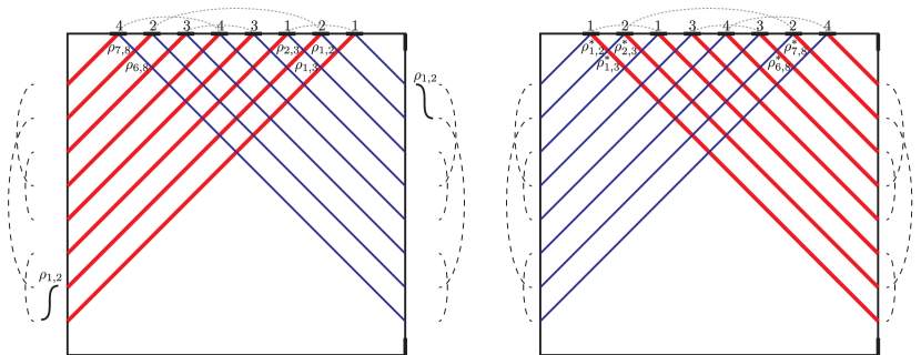
The Auroux-Zarev interpolating piece [Aur10, Zar10], is the --bordered Heegaard diagram defined as follows. For fixed , let be the triangle defined by the -axis, the -axis, and the line . Let be the edge of along the -axis, be the edge along the -axis, and be the diagonal edge. Produce a genus surface from by identifying small neighborhoods of the points and on whenever and are matched in . If and are matched in , the two vertical segments and descend to a single arc; declare this to be a -arc. Similarly, the two horizontal segments and descend to a single arc; declare this to be an -arc. Finally, attach a one-handle connecting small neighborhoods of and , giving a surface . Place the basepoint at . Then , and the boundary of is . See Figure 1.
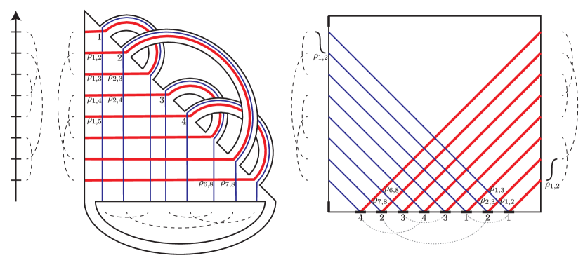
There is a canonical identification between the set of generators and the strand diagram basis for as follows [Aur10, LOT11]. Numbering the -arcs from the top and the -arcs from the left, the number of points in is two if and otherwise is equal to the number of chords in starting at an endpoint of and ending at an endpoint of . If the endpoints of are and , the intersection point in which lies on corresponds to the smeared horizontal strand . Other intersection points correspond to upward-sloping chords as follows: if lies at coordinates , then corresponds to the strand in . Figure 1 indicates the identifications between intersection points in and chords in . An arbitrary element of is a set of such intersection points, and corresponds to a strand diagram in .
Using the fact that is nice, it is easy to see that the differential on corresponds to the differential on . Furthermore, multiplications correspond to -tuples of half-strips on the appropriate boundary [LOT11, Proposition 8.4]. If we treat the boundary as the right action and the boundary as the left action, we have
whereas if we treat the boundary as the left action and the boundary as the right action, we have
In our computations in Section 4, we will use (for the split pointed matched circle), and treat the -boundary as the left action and the -boundary as the right action. Then,
The corresponding labeling of generators is shown in Figure 2.
We are also interested in a related diagram obtained from by switching the and curves. (Equivalently, one could reflect across the -axis, obtaining .) Let be the dual, over , of . Since comes with a preferred basis, the strand diagrams, there is a preferred basis for . The differential on is the transpose of the differential on . Moreover, has left and right multiplications by : on the right, is the element of which sends an element to , and on the left is the element of which sends an element to .
By the same computation as above one obtains
| (2.1) |
if the -action is on the right [LOT11, Appendix A]. See also Figure 2.
Next we describe in the case that the boundary gives the left type structure and the boundary gives the right type structure. From the pairing theorem,
Thus, a generator of corresponds to , where is a strand diagram in and is the complementary idempotent to the left idempotent of . The map is given by multiplication on the right; the image of is contained in the subspace . The map is given by
All higher operations , , vanish.
The same argument, but using Equation (2.1), leads to the following description of . As needed by our application, we will treat the boundary as the left action and the boundary as the right action. Generators of correspond to , where is a strand diagram in , is the corresponding basis element of and is the complementary idempotent to the left idempotent of (or, equivalently, the right idempotent of ). The map is given by . The map is given by
All higher operations , , vanish.
To conclude this section, we recall some gluing properties of the diagrams and from [LOT11]:
Lemma 2.2.
[LOT11, Corollary 4.5] The Heegaard diagram represents the identity map of , and the diagram represents the identity map of .
Lemma 2.3.
[LOT11, Corollary 4.6] Let be an -bordered Heegaard diagram for . Then the Heegaard diagram represents the three-manifold . In particular, and represent the same bordered three-manifold.
Convention 2.4.
In the rest of the paper, we will typically drop from the Auroux-Zarev piece, writing (respectively ) to denote or (respectively or ) as appropriate. Whether or is required is determined by the boundary of the diagram.
2.5. Gradings on bordered Floer modules
A key step in our computations is knowing that there are unique graded homotopy equivalences between certain modules and bimodules (as formulated in Section 4). Here we review enough of the gradings in bordered Floer homology to make this statement precise. More details can be found in the original papers [LOT08, Chapter 10], [LOT15, Sections 2.5, 3.2, 6.5].
Fix a pointed matched circle representing a surface . The algebra is graded by a group which is a central extension
Let be a generator for the central . For homogeneous elements , differential satisfies , and the multiplication satisfies .
Given a bordered -manifold with boundary parameterized by , is graded by a right -set , and is graded by a left -set . The -orbits in these sets correspond to the -structures on . Similarly, if is a cobordism from to then is graded by a set with a left action by and a right action by ; is graded by a set equipped with commuting left actions by and ; and is graded by a set equipped with commuting right actions by and . The group is the opposite group to , so a left -set is the same data as a right -set; and are related in this way. (Of course, all groups are isomorphic to their opposites, but here it is convenient to maintain the distinction.)
The -grading on the bordered (bi)modules depends on a choice of grading refinement data [LOT08, Section 10.5]. However, up to homotopy equivalence, the bordered invariants are independent of this choice [LOT15, Proposition 6.32].
The special cases of interest to us are:
-
(1)
Handlebodies. Suppose is a handlebody of genus . Then there is a unique -structure on . The corresponding -set is the quotient of by a subgroup isomorphic to , which projects isomorphically to . In particular, the grading element acts freely on .
-
(2)
Mapping cylinders of diffeomorphisms. If is a strongly based diffeomorphism and is the associated arced cobordism then is a free, transitive -set, and also a free, transitive -set. Similar statements hold for and .
Given type structures and , graded by -sets and , respectively, the chain complex of type structure morphisms inherits a grading by the -set [LOT15, Section 2.5.3], where is the right -set with elements in bijection with and action [LOT15, Definition 2.5.19]. The -action persists because is central in . The situation for -modules and the various types of bimodules is similar. A morphism is homogeneous if it lies in a single grading.
So, if acts transitively on the grading set for then the complex is graded by as -sets. A morphism has grading 0 if it lands in the summand corresponding to for some (or equivalently, any) .
Example 2.5.
Let be a -framed solid torus, and consider . Since , the gradings satisfy . Thus, the homomorphism , has degree .
3. Computation of homotopy equivalences
Two key steps in our descriptions of involutive Floer homology and the mapping class group involve computing homotopy equivalences between -modules or between type bimodules. We explain in this section that the bordered algebras have finiteness properties which imply that these computations can be carried out to any order desired.
Lemma 3.1.
Given a pointed matched circle there is an integer so that any product of chords in vanishes.
Proof.
This is immediate from the fact that no two strands in a strand diagram can start at the same point in the matched circle. So, if represents a surface of genus ,
suffices. (This bound is not optimal.) ∎
Proposition 3.2.
Fix a dg algebra and let and be type bimodules over and where is a pointed matched circle. Let be as in Lemma 3.1. Suppose and satisfy the type homomorphism relations with up to inputs. Then there is a type module homomorphism so that for all .
Since -modules are a special case of type bimodules, this proposition covers -modules as well. Roughly, the proposition says that, after building a homomorphism which takes up to inputs, one never gets stuck in extending the homomorphism to take one more input.
Proof of Proposition 3.2.
View as a left-right type structure over and . The functor gives an equivalence of categories from the category of type bimodules over and to the category of (left-right) type bimodules over and . This functor sends a morphism to . As we will see, the key point is that the form of the differential on and Lemma 3.1 imply that the map depends only on the terms for .
Fix data as in the statement of the proposition. Temporarily declare for , and form . It follows from Lemma 3.1 and the form of on (see also Section 2.3) that is a type structure homomorphism. Since is a homotopy equivalence of dg categories, there is a type structure homomorphism so that is homotopic to . So, is nullhomotopic, so is itself nullhomotopic. Let be a nullhomotopy of , i.e., . Write where consists of the terms with inputs and consists of the terms with inputs. Let . Then for all . Further,
so is a type structure homomorphism. This proves the result. ∎
Proposition 3.2 implies that if and are homotopy equivalent then one can compute a homotopy equivalence. First one finds terms with up to inputs satisfying the type structure relations with up to inputs, and so that this map has an up-to--input homotopy inverse. This is a finite (albeit huge) computation. Proposition 3.2 then implies that one can extend any such solution to more inputs, by solving the type structure relation inductively; one never gets stuck.
Maybe a final word is in order about the meaning of the word compute. We have finitely generated modules and with only finitely many non-zero operations. A type structure homomorphism from to is a computer program (Turing machine) which takes as input an integer and inputs and and gives as output an element of . Being able to compute means we can write a computer program which takes as inputs homotopy equivalent modules and and outputs a computer program representing a type homotopy equivalence from to .
4. Rigidity results
In this section we prove that, up to homotopy, there are unique homogeneous homotopy equivalences between certain modules. The results in this section were originally observed by P. Ozsváth, D. Thurston, and the second author.
We will call a map (and, in particular, a homotopy equivalence) homogeneous if is homogeneous with respect to the grading on morphism spaces (cf. Section 2.5).
Lemma 4.1.
Let be the -framed handlebody of genus and the standard type module for (as in Section 2.2). Then there is a unique homogeneous homotopy equivalence .
Proof.
Let be a homogeneous homotopy equivalence. Write
where the are strand diagrams (basic elements of ). Let denote the ideal spanned by strand diagrams not of the form (i.e., in which at least one strand is not horizontal). Then, as algebras,
Let be the result of extending scalars from to . Then is isomorphic to , with trivial differential. Since must induce a homotopy equivalence
it follows that one of the , say , is the idempotent . That is,
where .
Next we claim that . Since both the left and right idempotents of must agree with the left idempotent of , the are in the algebra generated by
As in Example 2.5,
Since is homogeneous and appears in , so every term in has the same grading as , it follows that and so . ∎
Suppose that is a Heegaard diagram for a bordered handlebody and is a -set graded type structure homotopy equivalent to . Then
[LOT11, Theorem 1] is graded by a free -set (cf. Section 2.5). Further, the homology lies over a single -orbit in the grading set. This -orbit inherits a total order, by declaring that if for some . Thus, it makes sense to talk about a nontrivial homomorphism (that is, a homomorphism whose image in is nontrivial) of maximal grading. The same discussion holds for type invariants.
Lemma 4.2.
Let be a Heegaard diagram for a bordered handlebody and (respectively ) a -set-graded type structure (respectively -module) homogeneous homotopy equivalent to . Then up to chain homotopy there is a unique homogeneous homotopy equivalence (respectively ). Further, this homotopy class is represented by any non-trivial homomorphism of maximal grading.
So, if and represent the same bordered handlebody, to find a homotopy equivalence , say, it suffices to find any grading-preserving, non-nullhomotopic homomorphism.
Proof.
First, if and are homotopy equivalent then the set of homotopy classes of homotopy equivalences from to is a torseur for the set of homotopy classes of homotopy equivalences from to . So, it suffices to prove the lemma in the case that and .
If represents the standard -framed handlebody then by Lemma 4.1 there is a unique homogeneous homotopy equivalence . Next, there is a mapping class so that represents a handlebody with boundary parameterized by . Then the pairing theorem gives a homogeneous homotopy equivalence
| (4.3) |
Tensoring with is an equivalence of homotopy categories of -set-graded type structures, with inverse [LOT15, Corollary 8.1], so the set of homotopy classes of homogeneous homotopy auto-equivalences of is in bijection with the set of homotopy classes of homogeneous homotopy auto-equivalences of . Thus, by Equation (4.3) there is a unique homotopy class of homogeneous homotopy auto-equivalences of . Finally,
Since tensoring with is an equivalence of homotopy categories, with inverse given by tensoring with [LOT15, Corollary 8.1], there is a unique homotopy class of homogeneous homotopy auto-equivalences of .
For the second part of the statement, observe that any other non-trivial homogeneous homomorphism has grading strictly smaller than the identity map. This property, too, is preserved by homotopy equivalences and equivalences of the homotopy category. ∎
There is an analogous result for the bimodules associated to mapping classes:
Lemma 4.4.
Let be the standard type bimodule for the trivial cobordism (as in Section 2.3). Then there is a unique homogeneous homotopy equivalence , which is also the unique nontrivial homomorphism of maximal grading.
Proof.
Since different choices of grading refinement data lead to graded chain homotopy equivalent modules [LOT15, Proposition 6.32], it suffices to prove the lemma for any choice of grading refinement data. Choose any grading refinement data for , and work with the induced grading refinement data for . With respect to these choices, all of the generators of are in the same grading.
Let be a homotopy equivalence. Write
where the and are strand diagrams. Note that for each , , and ,
Considering and as in the proof of Lemma 4.1 shows that for each generator , one of the terms must be . We claim that these are the only terms in .
To see this note that the fact that is homogeneous implies that the supports of and (in ) must be the same. (This statement depends on the fact that we are using corresponding grading refinement data for and .) That is, lies in the diagonal subalgebra [LOT14b, Definition 3.1]. Every basic element in the diagonal subalgebra can be factored as a product of chord-like elements [LOT14b, Lemma 3.5]. Since occurs in the differential on , it follows that the grading of a product of chord-like elements is . Thus, since is homogeneous, each term must be a product of chord-like elements, i.e., have the form . This proves the result. ∎
Lemma 4.5.
If is a mapping class and is a type bimodule homogeneous homotopy equivalent to (respectively , ) then there is a unique homogeneous homotopy equivalence between (respectively , ) and . Further, the homotopy equivalence is the unique non-zero homotopy class of homomorphisms of maximal grading.
Proof.
Since tensoring with gives an equivalence of homotopy categories, it suffices to prove the statement for . Further, since tensoring with gives an equivalence of categories, it suffices to prove the statement for . Since the number of homotopy equivalences is preserved by homotopy equivalences, it suffices to show there is a unique homotopy equivalence and that this homotopy equivalence is the unique non-nullhumotopic map of maximal grading. So, the result now follows from Lemma 4.4 and its proof. ∎
Corollary 4.6.
Up to homotopy, there is a unique homogeneous homotopy equivalence
Proof.
Since represents the identity diffeomorphism, this follows from the pairing theorem and Lemma 4.5. ∎
5. Involutive bordered Floer homology
We start by proving that the bordered description of in the introduction does, in fact, give :
Theorem 5.1.
Proof.
In outline, the proof is that, up to homotopy, the map in Formula (1.3) agrees with the map in the definition of , while the composition agrees with the map in the definition of . To check this we need to verify that:
-
(1)
Up to homotopy, the following diagram commutes:
(5.2) where the vertical arrows come from the pairing theorem for bordered Floer homology.
- (2)
(Note that the top-left square of Diagram (5.3) is canonically isomorphic to .)
The fact that Diagram (5.2) commutes is straightforward from either proof of the pairing theorem. For example, the time-dilation proof [LOT08, Chapter 9] has two steps. In the first, one chooses complex structures on with increasingly long necks around . For sufficiently large, the differential on agrees with a count of pairs of holomorphic curves in and , subject to a matching condition. We may as well assume that is computed with respect to one of these sufficiently large . One then deforms the matching condition and observes that after a sufficiently large deformation the resulting differential agrees with . Complexes with different deformation parameters are chain homotopy equivalent. Now, if one chooses the conjugate complex structure to on and then performs exactly the same deformation, at every stage the moduli spaces of holomorphic curves for and are identified. Thus, Diagram (5.2) can be chosen to commute on the nose. (The argument via the nice diagrams proof [LOT08, Chapter 8] is even simpler, and is left as an exercise.)
Consider next Diagram (5.5). By a similar argument to the one just given, it suffices to show that the corresponding diagram
homotopy commutes. Recall that is the box product of maps and , induced by Heegaard moves from to and from to , respectively. By definition, , but this is canonically homotopic to [LOT15, Section 3.2]. Thus, we can break this into two steps, by considering the diagram
The proofs of commutativity of the two squares are essentially the same, so we will focus on the left square. We can relate to by a sequence of bordered Heegaard moves; let be the sequence of bordered Heegaard diagrams obtained by doing these moves one at a time, with and . There is a corresponding sequence of closed Heegaard diagrams
each successive pair of which is related by a Heegaard move. So, it suffices to check that:
Lemma 5.6.
If and are bordered Heegaard diagrams related by a bordered Heegaard move and is another bordered Heegaard diagram with then the diagram
commutes up to homotopy. (Here, the horizontal arrows come from the invariance proofs for bordered and classical Heegaard Floer homology.)
Proof.
For stabilizations (near the basepoint ), this is obvious: if is the intersection point between the new -circle and the new -circle then both horizontal maps send a generator to , and none of the moduli spaces used to define the vertical maps are affected. For handleslides, both horizontal maps are defined by counting holomorphic triangles, and the fact that this diagram commutes up to homotopy is a special case of the pairing theorem for triangles [LOT14a]. For isotopies, commutativity follows by imitating the proof of the pairing theorem but with dynamic boundary conditions. ∎
Commutativity of Diagram (5.4) follows from a similar argument. Here, the horizontal maps come from a sequence of Heegaard moves relating the identity Heegaard diagram to the diagram . Working one Heegaard move at a time, the result follows from the obvious bimodule analogue of Lemma 5.6.
For Diagram (5.3), note that there are two homotopy equivalences
one given by a sequence of Heegaard moves from to and the pairing theorem, and the other given by tensoring with the homotopy equivalence . The second of these is the map , while for the first of these Diagram (5.3) clearly commutes. So, it suffices to show these two maps are homotopic. In the case that represents a handlebody, this follows from Lemma 4.2. For the general case, since tensoring with is a quasi-equivalence of dg categories, it suffices to show that the two maps
one induced by a sequence of Heegaard moves and the other induced by the equivalence , are homotopic. By homotopy associativity of the box tensor product and the pairing theorem (see [LOT15]), it suffices to show that the two maps
one given by a sequence of Heegaard moves and the other by the equivalence , are homotopic. This last statement follows from rigidity of , Lemma 4.4. ∎
Next we abstract the bordered information required to compute involutive Heegaard Floer homology.
Definition 5.7.
Fix a pointed matched circle . An involutive type module over consists of a pair where is a type structure over and
is a homotopy equivalence of type structures. We call two involutive type structures and equivalent if there is a type structure homotopy equivalence so that is homotopic to .
Similarly, an involutive -module over consists of a pair where is an -module over and
is a homotopy equivalence of -modules. We call involutive -modules and equivalent if there is an -module homotopy equivalence so that is homotopic to .
Definition 5.8.
Given a bordered -manifold with boundary and bordered Heegaard diagram for , let be the involutive type module where is the map
in which the first equivalence is given by the pairing theorem and the second is induced by some sequence of Heegaard moves from to .
Similarly, given a bordered -manifold with boundary and bordered Heegaard diagram for , let be the involutive -module where is the map
in which the first equivalence is given by the pairing theorem and the second is induced by some sequence of Heegaard moves from to .
Conjecture 5.9.
The involutive type structure and involutive -module are invariants of the bordered -manifold .
The missing ingredient to prove Conjecture 5.9 is an analogue of Ozsváth-Szabó-Juhász-Thurston-Zemke’s naturality theorem. That is, we do not know that the maps and are independent of the choice of sequence of Heegaard moves. In the special case that is a handlebody, Conjecture 5.9 follows from Lemma 4.2. In general, it is not even known that and are invariants of the Heegaard diagram , since as far as we know different sequences of Heegaard moves would give different maps and .
The rest of this paper does not depend on Conjecture 5.9.
Definition 5.10.
The tensor product
of an involutive type structure and an involutive -module is the mapping cone of the map
where is the homotopy equivalence from Corollary 4.6. This tensor product is a differential module over in an obvious way.
Lemma 5.11.
If and (respectively and ) are equivalent involutive type structures (respectively -modules) over then the box tensor products and are quasi-isomorphic differential modules over .
Proof.
The proof is straightforward and is left to the reader. ∎
The following is the pairing theorem for involutive bordered Floer homology:
Theorem 5.12.
Fix bordered Heegaard diagrams and with . Then there is a chain homotopy equivalence
Proof.
This follows from Theorem 5.1. ∎
6. Computing the mapping class group action
We start by recalling a well-known lemma:
Lemma 6.1.
Let be an orientation-preserving, based diffeomorphism. Then there is a Heegaard splitting with and a diffeomorphism isotopic to (rel. ) so that .
Proof.
Start with any Heegaard splitting of . Then is another Heegaard splitting of . Since any pair of Heegaard splittings becomes isotopic after sufficiently many stabilizations, after stabilizing enough times we may assume that is isotopic to , by some ambient isotopy . Consider the map . Since is isotopic to the identity, is isotopic to . Clearly preserves the Heegaard splitting . ∎
With notation as in the introduction, the main goal of this section is to prove:
Theorem 6.2.
The action of a mapping class on is given by the composition of the maps in Formula (1.4).
Proof.
The proof is similar to the proof of Theorem 5.1. Choose a Heegaard splitting as in Lemma 6.1. Let denote the Heegaard surface and the gluing diffeomorphism for the Heegaard splitting. Let be a bordered Heegaard diagram representing the -framed handlebody and a bordered Heegaard diagram representing , so is a Heegaard diagram for . Here, we view and as subsets of ; see Figure 3.
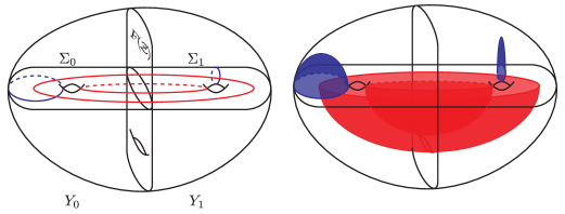
Applying to and gives new Heegaard diagrams for . (Abstractly, of course, these diagrams are diffeomorphic to the original ones, but they are new subsets of the manifolds .) Let denote the mapping cylinder of , and let be a bordered Heegaard diagram for . Cutting along and gluing in does not change the -manifold. At the level of Heegaard diagrams, this corresponds to gluing to and to . Further, this cutting and regluing can be realized by a path of Heegaard diagrams from the standard Heegaard diagram for the identity map to .
Now, and are bordered Heegaard diagrams representing , and the Heegaard surfaces are embedded so that they have the same boundary. Similarly, and both represent . Choose a path of Heegaard diagrams from to , and a path from to . By definition, the map on induced by comes from the composition of the Heegaard Floer continuation map associated to the path which introduces and then the Heegaard Floer continuation maps associated to the Heegaard moves from to and to .
By the pairing theorem for holomorphic triangle maps [LOT14a, Proposition 5.35], these continuation maps agree with the tensor products of the bordered continuation maps associated to the pieces which are changing. So, a similar argument to the proof of commutativity of Diagrams (5.3), (5.4), and (5.5) shows that the action of on is given by the composition
where the first map comes from the homotopy equivalence , the second map comes from some homotopy equivalence and the third map comes from some homotopy equivalences and . By Lemmas 4.2 and 4.5, up to homotopy there is a unique homotopy equivalence in each case. ∎
As noted in the introduction, each of the maps in Formula (1.4) is the unique homotopy class of homotopy equivalences between the given source and target. So, after computing the modules and bimodules by factoring into mapping classes [LOT14b], computing the homotopy equivalences required to describe the mapping class group action is straightforward (and, in particular, algorithmic).
7. The surgery exact triangle
The goal of this section is to prove:
Theorem 7.1.
Let be a framed knot in a -manifold . Then there is a surgery exact triangle
Before turning to the proof, to fix notation we recall the modules and maps used in the bordered proof of the surgery exact triangle for [LOT08, Section 11.2]. (The reader is referred to the original paper for a more leisurely account.)
Let , and be the standard, genus Heegaard diagrams for the -framed, -framed, and -framed solid tori, respectively. It is easy to compute that
Further, there is a short exact sequence
where and are given by
Given any bordered -manifold with boundary , tensoring this short exact sequence with gives a long exact sequence in homology [LOT08, Proposition 2.36]—the desired surgery exact sequence. (This exact sequence agrees with Ozsváth-Szabó’s original [OSz04a], as proved in [LOT14a, Corollary 5.41].)
For notational convenience, in this section let . The main work in extending these bordered computations to prove Theorem 7.1 is the following lemma:
Lemma 7.2.
There are homotopies and making each square of the following diagram homotopy commute:
Further, .
Proof.
This is a direct computation.
Recall from Section 2.4 that is the type bimodule with generators
The operation is the obvious right action of , and is induced by
and the Leibniz rule with . All higher , , vanish.
Thus, the type structure has generators
(as a type structure) with differential given by
Here, some terms come from the operation on (together with the operation on ) while other terms come from the operation on . The quasi-isomorphism is given by
These formulas are perhaps easier to absorb, and check, graphically:
Here, we have replaced tensor signs with vertical bars. Unlabeled arrows are implicitly labeled by idempotents. Dashed arrows represent the map , while solid arrows represent . Labels are always above the corresponding arrows. The check that is a homomorphism reduces to examining all length-two paths from a vertex on the left to . The map is clearly a quasi-isomorphism.
After this warm-up, the complexes and ; the maps on them; the morphisms and and induced maps and ; and the homotopies are shown in Figure 4.
Again, checking that this diagram is correct reduces to looking at length-two paths. Have fun! ∎
Proof of Theorem 7.1.
The framing of makes into a bordered -manifold. We claim that the squares in the following diagram commute up to the dashed homotopies shown:
Indeed, the fact that the top two rows commute on the nose follows from basic properties of the box tensor product [LOT15, Lemma 2.3.3]. For the third row, commutativity up to the homotopies follows from these properties and Lemma 7.2. Further, by Lemma 7.2, the homotopies satisfy
Since by Theorem 5.1 the composition of the three vertical arrows in any column is the map , it follows that there is a homotopy commutative diagram
| (7.3) |
where the rows are short exact sequences inducing the surgery exact triangle on homology, and the diagonal arrows are the homotopies and .
The theorem now follows from the commutative diagram (7.3) and homological algebra (cf. [HM17, Proof of Proposition 4.1]). That is, by Lemma 7.2, the homotopies in Diagram (7.3) satisfy
| (7.4) |
Take the mapping cone of each vertical map in the diagram, to obtain a sequence of chain complexes
where the maps are given by the matrices
Homotopy commutativity of Diagram (7.3) implies that these maps are chain maps, and exactness of the rows in Diagram (7.3) together with Equation (7.4) implies that this sequence is exact. The associated long exact sequence is the statement of the lemma. ∎
Remark 7.5.
The proof of Theorem 7.1 also shows that the map induced by on homology commutes with the maps in the surgery exact triangle for . Lidman points out that this commutativity can be deduced more directly, by an argument that also applies to . Specifically, the maps in the surgery exact triangle for or are induced by cobordisms, and cobordism maps commute with the conjugation isomorphism (cf. [OSz06, Theorem 3.6]).
8. Involutive Floer homology as morphism spaces
In this section we give some formulas purely in terms of for the map and the map associated to a mapping class, which may be helpful in computer implementations.
Given a type structure over a dg algebra over , consisting of a finite-dimensional underlying vector space and a map , the dual type structure has underlying vector space , the dual space to , and operation
induced from via the identifications
Given a bordered -manifold with boundary , recall that
[LOT11, Theorem 2] so given bordered -manifolds and with ,
| (8.1) |
[LOT11, Theorem 1].
Using this, we explain how to compute the map without mentioning . Fix a Heegaard splitting . To compute one first computes and , where is the -framing (as in Section 2.2). The computation of uses a factorization of into arcslides and the identity
(see [LOT14b]). Then one uses Formula (8.1). Indeed, this algorithm has already been implemented by Lipshitz-Ozsváth-Thurston [LOT14b] and Zhan [Zha].
Recall that a bimodule is called quasi-invertible if there is a bimodule so that
Let denote the complex of left type morphisms of . This morphism complex is an -bimodule. (The module structure is somewhat intricate; see [LOT15, Section 2.3.4].)
We have the following Yoneda lemma:
Lemma 8.2.
Let and be dg algebras and a quasi-invertible bimodule. Then there is a quasi-isomorphism of -bimodules
which sends the multiplicative identity to the identity morphism . More generally, the -bimodule map is given by
| (8.3) |
where is the structure map of .
Proof.
Let be the chain complex of type structure morphisms. Then the map defined by
is a chain homotopy equivalence. Next, since is quasi-invertible, the functor is a quasi-equivalence of dg categories. Thus, the map
is a quasi-isomorphism. (Compare [LOT15, Proposition 2.3.36].) The composition is the desired equivalence. Tracing through the definitions gives the Formula (8.3). ∎
Corollary 8.4.
Under the identification
the unique homogeneous homotopy equivalence (of -bimodules)
is given by
Proof.
This is immediate from Lemma 8.2 and the fact that the structure map for vanishes for . ∎
Theorem 8.5.
Fix a Heegaard splitting of . Then up to homotopy the map is given by the composition
where
sends a morphism to and, if is the homogeneous homotopy equivalence, then sends a morphism to .
This seems to be a succinct, and computer-friendly, description of the map .
Proof.
Choose a Heegaard diagram for . Then the pairing theorem gives
which is identified, via, , with
Similarly,
Consider a sequence of Heegaard moves
where the first arrow does not change the diagrams at the end and the second arrow consists of bordered Heegaard moves changing the diagrams on the two sides of the big union sign. There are two associated maps on . By the pairing theorem for triangles, the first map is induced by a map
By uniqueness, this map is the map of Corollary 8.4. It follows from the definition of and the pairing theorem that the induced map
sends to . Similarly, by the pairing theorem for triangles, the second map is induced by an equivalence on each of the parenthesized pieces, and thus agrees with the map . ∎
The mapping class group action admits a similar description: the action of is given by
where the first map sends a morphism to and the second sends to . We can rewrite this using instead of as
where the first arrow sends a morphism to the morphism which sends a morphism to and the second arrow is again induced by the unique homotopy equivalences and . The proof that this gives the mapping class group action is similar to the proof of Theorem 8.5 and is left to the reader.
9. Examples
For a knot in , let denote the branched double cover of . To illustrate the algorithm for computing , we finish the computation of for knots through crossings.
If is an -space then, since is a rational homology sphere with a unique -structure, . That is, has two generators for each conjugacy class of -structures. The -action takes one generator corresponding to the -structure to the other, and vanishes on all other generators. All knots with or fewer crossings have an -space. Indeed, except for , and , every knot with or fewer crossings is quasi-alternating [JS09, Jab14]; for quasi-alternating knots, is an -space [OSz05]. It turns out that , and are -spaces. (This can be checked using Zhan’s computer program [Zha].)
The -crossing knots for which is not an -space are listed in Table 1. The computation of which of these spaces are not -spaces, and the dimensions of their Floer homologies, was accomplished by Zhan. Computation of for these manifolds was carried out by a modest extension of Zhan’s program, using the algorithm described above. The first two knots, and , are Montesinos knots, hence our our computation is implied by (and agrees with) the computation of for Seifert fibered spaces [DM17]. We make a few further comments about the details of our implementation below.
| Knot | |||
|---|---|---|---|
| 3 | 5 | 6 | |
| 3 | 5 | 6 | |
| 11 | 13 | 14 | |
| 1 | 5 | 6 | |
| 13 | 15 | 16 | |
| 5 | 7 | 8 |
Both Zhan’s code and our extension, which is now included in Zhan’s package [Zha], are written in Python (version 2.7). Zhan’s code includes classes for chain complexes, type structures, and type structures, as well as for morphisms between them. He also, of course, implemented basic operations on these structures, including taking the box tensor product of a type structure and a type structure and computing the morphism complex between two type structures. His program also automates computation of given a bridge diagram for . The algorithms behind Zhan’s code use properties of the bordered bimodules which appear only in his thesis [Zha14] to compute tensor products without writing down all of the generators. (He calls this technique extending by the identity and the local objects that he extends local type structures.) The upshot is that his code computes and efficiently.
In our extension, we implemented the bimodule , mapping cones of maps between type structures and chain complexes, composition of morphisms between type structures, and the tensor product of a morphism of type structures with the identity map of a type structure. Computing mapping cones gives some easy sanity checks: it makes testing whether maps are quasi-isomorphisms trivial, by checking whether their mapping cones are acyclic.
Our code computes the rank of by:
-
(1)
Computing , , , and , as well as various morphism complexes between them.
-
(2)
Computing a basis for , consisting of explicit cycles in .
-
(3)
For each basis element , computing .
-
(4)
Computing a basis for and for . Even though we do not implement the grading for , the way that Zhan’s code computes homology automatically gives bases of homogeneous elements. Each of these bases has elements where is the genus of the Heegaard splitting. For the computations in Table 1, , so each of these bases has elements.
-
(5)
Searching through these bases to find the unique homotopy equivalences and .
-
(6)
For each , computing the composition . The map
is a map
representing . (Mapping from the homology of the complex to the complex means we do not have to choose a projection from the morphism complex to its homology.) Abusing notation, we call this map .
-
(7)
There is also an inclusion
induced by the choice of cycles . The involutive Floer homology is then the homology of .
The computations in Table 1 are fairly slow: on a circa 2016 MacBook Pro with 16 GB of RAM the code computes within a few minutes but each computation of takes up to several hours. (We have not made a serious attempt to improve the efficiency of our code.)
9.1. Computing from
Sometimes, one can recover from and . (This is desirable given that most known applications use or rather than .) We illustrate the process of recovering by computing up to a grading shift.
Let denote the -structure on . If is any other -structure then, since , with trivial -action, where denotes the orbit consisting of the structure and its conjugate. So, for the rest of the section we focus on .
Lemma 9.1.
Let be the Heegaard Floer correction term of the -structure on . Then
with -action given by and .
In [HM17], C. Manolescu and the first author extract two invariants of -homology cobordism from involutive Heegaard Floer homology, called the involutive correction terms. Given a rational homology sphere and a conjugation-invariant -structure , in terms of the minus variant, these invariants are
and
We therefore have the following corollary of Lemma 9.1:
Corollary 9.2.
The involutive correction terms of in the unique structure are related to by
Proof of Lemma 9.1.
Let . Zhan’s code for computing can be used to compute relative gradings and -structures for generators of . Arbitrarily numbering the -structures of the generators by , the code finds that, up to a shift, the gradings of the generators representing the different -structure are:
| 3 | 6/5 | 0 | 2/5 | |
| 3 | 6/5 | 1 | 2/5 | |
| 3 | 1/5 | 2 | 0 | |
| 4 | 0 |
Thus, the -structure labeled must be the central -structure. From the computer computation, , so must have exactly one fixed point, which must be the generator in relative grading . The other two elements in this -structure must, up to a change of basis, be interchanged by . We conclude that contains three elements, two in some grading and one in grading , and that up to a change of basis, the two elements in grading are interchanged by .
Now, recall that there is a long exact sequence
| (9.3) |
such that the map increases the grading by and the map decreases the grading by [OSz04a, Proposition 2.1]. This long exact sequence commutes at every step with [HM17, Proof of Proposition 4.1]. (Strictly speaking, this was proved for the analogous sequence for , but the proof for is identical.) It follows from the existence of this long exact sequence that there is a noncanonical isomorphism , where both and lie in grading . In particular, the ordinary Heegaard Floer correction term is . Further, the grading shifts imply that the summand of in grading is precisely the image of the summand of in grading , which is spanned as a vector space by and . Therefore since the long exact sequence (9.3) respects the action , the involution on is determined by the involution on . There are exactly two -equivariant involutions on : the identity and the involution , . The first of these induces the identity involution on , contradicting the computer computation. Thus, , .
Ordinarily, the existence of this triangle is insufficient to determine . (That is, is in general not a mapping cone of the map on , unlike the hat variant.) However, in this case the complex is sufficiently small that given our computation of , the mapping cone of is the unique -module that fits into the long exact triangle. The map takes to . So, is generated by , , and , and those elements lie in gradings , , and respectively. ∎
Remark 9.5.
The reader may have noticed that the complex is (after a change of basis) a symmetric graded root. Indeed, I. Dai and C. Manolescu recently showed that whenever is such that is a symmetric graded root with involution given by the canonical symmetry, is a mapping cone on [DM17, Theorem 1.1].
Remark 9.6.
It may be interesting to compare these computations with Lin’s spectral sequence from a variant of Khovanov homology to involutive monopole Floer homology of the branched double cover [Lin16a].
Remark 9.7.
One could call a rational homology sphere -trivial if for each -structure on , where and is non-vanishing on the remaining generator. At the time of writing, no -nontrivial rational homology sphere is known.
References
- [Aur10] Denis Auroux, Fukaya categories of symmetric products and bordered Heegaard-Floer homology, J. Gökova Geom. Topol. GGT 4 (2010), 1–54, arXiv:1001.4323.
- [BH16] Maciej Borodzik and Jennifer Hom, Involutive Heegaard Floer homology and rational cuspidal curves, 2016, arXiv:1609.08303.
- [DM17] Irving Dai and Ciprian Manolescu, Involutive Heegaard Floer homology and plumbed three-manifolds, 2017, arXiv:1704.02020.
- [HLS16] Kristen Hendricks, Robert Lipshitz, and Sucharit Sarkar, A flexible construction of equivariant Floer homology and applications, J. Topol. 9 (2016), no. 4, 1153–1236.
- [HM17] Kristen Hendricks and Ciprian Manolescu, Involutive Heegaard Floer homology, Duke Math. J. 166 (2017), no. 7, 1211–1299.
- [HMZ17] Kristen Hendricks, Ciprian Manolescu, and Ian Zemke, A connected sum formula for involutive Heegaard Floer homology, Selecta Math. (2017), 1–63, DOI:10.1007/s00029-017-0332-8.
- [Jab14] Slavik Jablan, Tables of quasi-alternating knots with at most 12 crossings, 2014, arXiv:1404.4965.
- [JS09] Slavik Jablan and Radmila Sazdanović, Quasi-alternating links and odd homology: computations and conjectures, 2009, arXiv:0901.0075.
- [JT12] András Juhász and Dylan P. Thurston, Naturality and mapping class groups in Heegaard Floer homology, 2012, arXiv:1210.4996.
- [Kho06] Mikhail Khovanov, An invariant of tangle cobordisms, Trans. Amer. Math. Soc. 358 (2006), no. 1, 315–327.
- [Lin14] Francesco Lin, A Morse-Bott approach to monopole Floer homology and the Triangulation conjecture, 2014, arXiv:1404.4561.
- [Lin15] Jianfeng Lin, Pin(2)-equivariant KO-theory and intersection forms of spin 4-manifolds, Algebr. Geom. Topol. 15 (2015), no. 2, 863–902.
- [Lin16a] Francesco Lin, Khovanov homology in characteristic two and involutive monopole Floer homology, 2016, arXiv:1610.08866.
- [Lin16b] by same author, Manolescu correction terms and knots in the three-sphere, 2016, arXiv:1607.05220.
- [Lin17a] by same author, -monopole Floer homology, higher compositions and connected sums, J. Topol. 10 (2017), no. 4, 921–969.
- [Lin17b] by same author, The surgery exact triangle in -monopole Floer homology, Algebr. Geom. Topol. 17 (2017), no. 5, 2915–2960.
- [LOT08] Robert Lipshitz, Peter S. Ozsváth, and Dylan P. Thurston, Bordered Heegaard Floer homology: Invariance and pairing, 2008, arXiv:0810.0687v4.
- [LOT11] Robert Lipshitz, Peter S. Ozsváth, and Dylan P. Thurston, Heegaard Floer homology as morphism spaces, Quantum Topol. 2 (2011), no. 4, 381–449, arXiv:1005.1248.
- [LOT14a] Robert Lipshitz, Peter S. Ozsváth, and Dylan P. Thurston, Bordered Floer homology and the spectral sequence of a branched double cover II: the spectral sequences agree, J. Topol. 9 (2014), no. 2, 607–686, arXiv:1404.2894.
- [LOT14b] by same author, Computing by factoring mapping classes, Geom. Topol. 18 (2014), no. 5, 2547–2681, arXiv:1010.2550v3.
- [LOT15] Robert Lipshitz, Peter S. Ozsváth, and Dylan P. Thurston, Bimodules in bordered Heegaard Floer homology, Geom. Topol. 19 (2015), no. 2, 525–724.
- [Man14] Ciprian Manolescu, On the intersection forms of spin four-manifolds with boundary, Math. Ann. 359 (2014), no. 3-4, 695–728.
- [Man16] by same author, Pin(2)-equivariant Seiberg-Witten Floer homology and the triangulation conjecture, J. Amer. Math. Soc. 29 (2016), no. 1, 147–176.
- [OSz04a] Peter S. Ozsváth and Zoltán Szabó, Holomorphic disks and three-manifold invariants: properties and applications, Ann. of Math. (2) 159 (2004), no. 3, 1159–1245, arXiv:math.SG/0105202.
- [OSz04b] by same author, Holomorphic disks and topological invariants for closed three-manifolds, Ann. of Math. (2) 159 (2004), no. 3, 1027–1158, arXiv:math.SG/0101206.
- [OSz05] by same author, On the Heegaard Floer homology of branched double-covers, Adv. Math. 194 (2005), no. 1, 1–33, arXiv:math.GT/0309170.
- [OSz06] by same author, Holomorphic triangles and invariants for smooth four-manifolds, Adv. Math. 202 (2006), no. 2, 326–400, arXiv:math.SG/0110169.
- [Sto15a] Matthew Stoffregen, Manolescu invariants of connected sums, 2015, arXiv:1510.01286.
- [Sto15b] by same author, Pin(2)-equivariant Seiberg-Witten Floer homology of Seifert fibrations, 2015, arXiv:1505.03234.
- [Sto17] Matthew Stoffregen, A remark on -equivariant Floer homology, Michigan Math. J. 66 (2017), no. 4, 867–884.
- [SW10] Sucharit Sarkar and Jiajun Wang, An algorithm for computing some Heegaard Floer homologies, Ann. of Math. (2) 171 (2010), no. 2, 1213–1236, arXiv:math/0607777.
- [Zar10] Rumen Zarev, Joining and gluing sutured Floer homology, 2010, arXiv:1010.3496.
- [Zem16] Ian Zemke, Connected sums and involutive knot Floer homology, 2016, arXiv:1705.01117.
- [Zha] Bohua Zhan, bfhpython, github.com/bzhan/bfhpython.
- [Zha14] by same author, Combinatorial methods in bordered Heegaard Floer homology, ProQuest LLC, Ann Arbor, MI, 2014, Thesis (Ph.D.)–Princeton University.