Inference in Deep Networks in High Dimensions

Abstract

Deep generative networks provide a powerful tool for modeling complex data in a wide range of applications. In inverse problems that use these networks as generative priors on data, one must often perform inference of the inputs of the networks from the outputs. Inference is also required for sampling during stochastic training of these generative models. This paper considers inference in a deep stochastic neural network where the parameters (e.g., weights, biases and activation functions) are known and the problem is to estimate the values of the input and hidden units from the output. While several approximate algorithms have been proposed for this task, there are few analytic tools that can provide rigorous guarantees on the reconstruction error. This work presents a novel and computationally tractable output-to-input inference method called Multi-Layer Vector Approximate Message Passing (ML-VAMP). The proposed algorithm, derived from expectation propagation, extends earlier AMP methods that are known to achieve the replica predictions for optimality in simple linear inverse problems. Our main contribution shows that the mean-squared error of ML-VAMP can be exactly predicted in a certain large system limit where the numbers of layers is fixed and weight matrices are random and orthogonally-invariant with dimensions that grow to infinity. ML-VAMP is thus a principled method for output-to-input inference in deep networks with a rigorous and precise performance achievability result in high dimensions.

I Introduction

Deep neural networks are increasingly used for describing probabilistic generative models of complex data such as images, audio and text [1, 2, 3]. In these models, data $\mathbf{y}$ is typically represented as the output of a feedforward neural network with randomness in the input. Randomness may also appear in the hidden layers. This work considers the inference problem for such a network, where the parameters are known (i.e., already trained) and we are to estimate the values of the inputs and hidden units from output data values $\mathbf{y}$.

Inference tasks of this form arise in inverse problems where a deep network is used as a generative prior for the data (such as an image) and additional layers are added to model the measurements (such as blurring, occlusion or noise) [4, 5]. Inference can then be used to reconstruct the original image from the measurements and provides an alternative to direct training for reconstruction [6]. Also, in unsupervised learning of the parameters of a generative network, one must sample from the posterior density of the hidden variables to perform stochastic gradient descent or EM [1, 2, 7].

While inference is most commonly a feedforward operation (given a new input, we compute the output of the network to make a classification or other prediction decision), here we are considering the inference problem in the reverse direction where we need to infer the input from the output. Although optimal output-to-input inference is generally intractable due to the nonlinear nature of neural networks, there are several methods that have worked well in practice. For example, MAP estimation can be performed by gradient descent on the negative log likelihood where the gradients can be computed efficiently from backpropagation and has been successful for problems such as inpainting [4, 5]. Approximate inference can also be performed via a separate learned deep network as is done in variational autoencoders [1, 2] and adversarial networks [8]. See also, [9]. However, similar to the situation in deep learning in general, there are few analytic tools for understanding how these algorithms perform or how far the estimates are from optimal.

In this work, we address this shortcoming by considering inference based on approximate message passing (AMP) [10, 11]. AMP methods are a class of expectation propagation (EP) techniques [12] that perform inference by attempting to minimize an approximation to the Bethe Free Energy [13, 14]. In addition to their computational simplicity, AMP methods have the benefit that the reconstruction error can be precisely characterized in certain high-dimensional random settings. Moreover, under further assumptions, they can provably obtain the Bayesian optimal performance as predicted by the replica method [15, 16, 17] – see, also [18]. Since their original work in sparse linear inverse problems [10, 11], AMP techniques have been successfully used to obtain rigorous theoretical guarantees in a wide range of settings including generalized linear models [19], clustering [20], finding hidden cliques [21] and matrix factorization [22].

A recent extension of these methods, called multi-layer AMP, has been proposed for inference in deep networks [23]. That work characterizes the replica prediction for optimality in multi-layer networks and argues that the proposed ML-AMP method can achieve this optimal inference in certain scenarios. Unfortunately, the convergence of ML-AMP in [23] is not rigorously proven. In addition, ML-AMP assumes Gaussian i.i.d. weight matrices $\mathbf{W}_{\ell}$, and it is well-known that AMP methods often fail to converge when this assumption does not hold [24, 25, 26, 27, 28].

In this work, we propose a novel AMP method called multi-layer vector AMP (ML-VAMP) that builds on the recent VAMP method of [29] and its extensions to GLMs in [30, 31]. The VAMP algorithm of [29] was itself derived from the expectation consistent approximate inference framework of [32, 33, 34] and applies to the special case of a linear problem. The ML-VAMP algorithm proposed here extends the VAMP method to networks with multiple layers and nonlinearities. Prior works in EP techniques for neural networks such as [35, 36] apply to the learning problem, not the inference problem considered here.

We analyze ML-VAMP in a setting where the number of layers is fixed and the weight matrices are random and orthogonally invariant with dimensions that grow to infinity. This class is much larger than the Gaussian i.i.d. matrices. Importantly, it includes weight matrices with arbitrary condition numbers, which is known to be the main failure mechanism in conventional AMP convergence [24]. Our main theoretical contribution (Theorem 1) shows that the mean squared error (MSE) of ML-VAMP algorithm can be precisely predicted by a simple set of scalar state evolution (SE) equations. The SE equations relate the achievable MSE to the key parameters of the network including the statistics of the weight matrices and bias vectors, their dimensions, the noise terms and activation functions. In this way, we develop a principled algorithm that enables computationally tractable inference with rigorous analysis of its achievable performance and convergence.

Our methods for analyzing inference algorithms bear some similarities with related recent theoretical analyses in deep learning. For example, [37] have shown that deep networks can be interpreted as max-sum inference on a certain deep rendering network. The work [38] studies the dynamics of gradient descent learning in a deep linear network. Interestingly, this work uses a singular value decomposition (SVD) of the weight matrices in the analysis, which is critical in our analysis as well. Also, [39] uses a large random weight matrix model in analyzing the the geometry of the loss function. This model is similar to the large system limit considered here. However, these methods all consider the more challenging problem of learning deep networks. In the inference problem considered here, the parameters of the network are already known and we only need to estimate the input and hidden states. In this regard, we can think of this inference problem as a simpler starting point for understanding deep learning methods.

II ML-VAMP Algorithm

II-A Algorithm Overview

We consider the following $M$-layer stochastic generative neural network model for data: A random input $\mathbf{z}_{0}$ with some density $p(\mathbf{z}_{0})$ generates a sequence of vectors, $\mathbf{z}_{\ell}$, $\ell=1,\ldots,L$, $L=2M$, through operations of the form,

$$\mathbf{z}_{\ell} =\mathbf{W}_{\ell}\mathbf{z}_{\ell\!-\!1}+\mathbf{b}_{\ell}+{\bm{\xi}}_{\ell},\quad {\bm{\xi}}_{\ell}\sim{\mathcal{N}}(\mathbf{0},\nu_{\ell}^{-1}\mathbf{I}),\quad \ell=1,3,\ldots,2M-1$$ (1a)

$$\mathbf{z}_{\ell} ={\bm{\phi}}_{\ell}(\mathbf{z}_{\ell\!-\!1},{\bm{\xi}}_{\ell}),\quad {\bm{\xi}}_{\ell}\sim p({\bm{\xi}}_{\ell}),\quad \ell=2,4,\ldots,2M.$$ (1b)

The updates (1a) are the linear stages of the network and are defined by weight matrices $\mathbf{W}_{\ell}$, bias vectors $\mathbf{b}_{\ell}$ and Gaussian noise terms ${\bm{\xi}}_{\ell}$. The updates (1b) are the nonlinear stages and are defined with activation functions $\phi_{\ell}(\cdot)$ such as a sigmoid or rectified linear unit (ReLU). The vectors ${\bm{\xi}}_{\ell}$ are noise terms to model randomness in each stage. The final output $\mathbf{y}=\mathbf{z}_{L}$ is the final (observed) data. We consider the output-to-input inference problem, where we are to estimate all the hidden variables in the network $\mathbf{z}_{\ell}$, $\ell=0,\ldots,L\!-\!1$ from the output $\mathbf{y}=\mathbf{z}_{L}$. Importantly, the weight matrices, bias terms, and activation functions $\phi_{\ell}(\cdot)$ are known (i.e. already trained). Thus, we are not looking at the learning problem.

The proposed ML-VAMP algorithm for this inference problem is shown in Algorithm 1. It can be derived as an extension of the GEC-SR algorithm of [30] which is used for inference in a GLM, which is the special case of the multi-layer problem with $L=2$. We assume a Bayesian setting where the initial condition $\mathbf{z}_{0}$ and noise terms ${\bm{\xi}}_{\ell}$ are independent random vectors, so the sequence $\mathbf{z}_{\ell}$ in (1) is Markov. The joint density of the variables $\mathbf{z}_{\ell}$ can then be written as

$$\mathbf{p}(\mathbf{z}_{0},\ldots,\mathbf{z}_{L})=p(\mathbf{z}_{0})\prod_{\ell=0}^{L\!-\!1}p(\mathbf{z}_{\ell\!+\!1}|\mathbf{z}_{\ell}),$$ (2)

where the transition probabilities $p(\mathbf{z}_{\ell\!+\!1}|\mathbf{z}_{\ell})$ are defined implicitly by the updates in (1). This density can be represented as a factor graph with $L+1$ factors corresponding to the terms $p(\mathbf{z}_{0})$ and $p(\mathbf{z}_{\ell+1}|\mathbf{z}_{\ell})$, $\ell=0,\ldots,L-1$. Since the final variable $\mathbf{z}_{L}=\mathbf{y}$ is observed, we have $L$ hidden variables $\mathbf{z}_{0},\ldots,\mathbf{z}_{L\!-\!1}$. This creates a linear graph.

Similar to the GEC-SR algorithm, the ML-VAMP algorithm shown in Algorithm 1 passes messages in the forward and reverse directions along the graph. The values $\mathbf{r}^{+}_{k\ell}$ and $\gamma^{+}_{k\ell}$ represent the mean and precision (inverse variance) values in the forward direction, and $\mathbf{r}^{+}_{k\ell}$ and $\gamma^{-}_{k\ell}$ are the values in the reverse direction. The formulae for the updates can be derived almost exactly the same as those in the GEC-SR algorithm [30] and are also similar to those in [29, 34]. We thus simply repeat the formulae without derivation. To update the messages, at each factor node $\ell=1,\ldots,L\!-\!1$ in the “middle" of the factor graph, we compute a belief estimate, which is a probability density

$$b_{\ell}(\mathbf{z}_{\ell},\mathbf{z}_{\ell\!-\!1}|\mathbf{r}^{+}_{\ell\!-\!1},\mathbf{r}^{-}_{\ell},\gamma^{+}_{\ell\!-\!1},\gamma^{-}_{\ell})\propto\exp\left[-H_{\ell}(\mathbf{z}_{\ell},\mathbf{z}_{\ell\!-\!1})\right],$$ (3)

where $H_{\ell}(\cdot)$ is the energy function

$$H_{\ell}(\mathbf{z}_{\ell},\mathbf{z}_{\ell\!-\!1}):=-\ln p(\mathbf{z}_{\ell}|\mathbf{z}_{\ell\!-\!1})+\frac{\gamma^{-}_{\ell}}{2}\|\mathbf{z}_{\ell}-\mathbf{r}^{-}_{\ell}\|^{2}+\frac{\gamma^{+}_{\ell\!-\!1}}{2}\|\mathbf{z}_{\ell\!-\!1}-\mathbf{r}^{-}_{\ell\!-\!1}\|^{2}.$$ (4)

At each iteration $k$, the belief estimates (3) with the values $\mathbf{r}^{+}_{k,\ell\!-\!1}$, $\mathbf{r}^{-}_{k\ell}$, $\gamma^{+}_{k,\ell\!-\!1}$ and $\gamma^{-}_{k\ell}$ represent the estimates of the posterior density $p(\mathbf{z}_{\ell\!-\!1},\mathbf{z}_{\ell}|\mathbf{x})$. We define the estimation functions $\mathbf{g}^{\pm}_{\ell}(\cdot)$ as the functions that compute the expected values of $\mathbf{z}_{\ell\!-\!1}$ and $\mathbf{z}_{\ell}$ with respect to these densities,

$$\mathbf{g}_{\ell}^{+}(\mathbf{r}^{+}_{\ell\!-\!1},\mathbf{r}^{-}_{\ell},\gamma^{+}_{\ell\!-\!1},\gamma^{-}_{\ell})=\mathbb{E}\left[\mathbf{z}_{\ell}|\mathbf{r}^{+}_{\ell\!-\!1},\mathbf{r}^{-}_{\ell},\gamma^{+}_{\ell\!-\!1},\gamma^{-}_{\ell}\right],$$ (5a)

$$\mathbf{g}_{\ell}^{-}(\mathbf{r}^{+}_{\ell\!-\!1},\mathbf{r}^{-}_{\ell},\gamma^{+}_{\ell\!-\!1},\gamma^{-}_{\ell})=\mathbb{E}\left[\mathbf{z}_{\ell\!-\!1}|\mathbf{r}^{+}_{\ell\!-\!1},\mathbf{r}^{-}_{\ell},\gamma^{+}_{\ell\!-\!1},\gamma^{-}_{\ell}\right],$$ (5b)

where the expectations are with respect to the belief estimates (3). For the end points $\ell=0$ and $L$ in the factor graph, we define the belief estimates

$$b_{0}(\mathbf{z}_{0}|\mathbf{r}^{-}_{0},\gamma^{-}_{0}),\quad b_{L}(\mathbf{z}_{L\!-\!1}|\mathbf{r}^{+}_{L\!-\!1},\gamma^{+}_{L\!-\!1}),$$

similar to (3) but with the terms from the left of the $\ell=0$ factor node or right of the $\ell=L$ factor node removed.

Algorithm 1 ML-VAMP

0:  Forward estimation functions $g_{\ell}^{+}(\cdot)$, $\ell=0,\ldots,L\!-\!1$ and reverse estimation functions $\mathbf{g}_{\ell}^{-}(\cdot)$, $\ell=1,\ldots,L$.

1:  Initialize $\mathbf{r}^{-}_{0\ell}$, $\gamma^{-}_{0\ell}$

2:  for $k=0,1,\dots,N_{\rm it}-1$ do

3:     // Forward Pass

4:     for $\ell=0,\ldots,L\!-\!1$ do

5:        if $\ell=0$ then

6:           $\widehat{\mathbf{z}}^{+}_{k\ell}=\mathbf{g}_{\ell}^{+}(\mathbf{r}^{-}_{k\ell},\gamma^{-}_{k\ell})$

7:           $\alpha^{+}_{k\ell}={\langle\partial\mathbf{g}_{\ell}^{+}(\mathbf{r}^{-}_{k\ell},\gamma^{-}_{k\ell})/\partial\mathbf{r}^{-}_{k\ell}\rangle}$

8:        else

9:           $\widehat{\mathbf{z}}^{+}_{k\ell}=\mathbf{g}_{\ell}^{+}(\mathbf{r}^{+}_{k,\ell\!-\!1},\mathbf{r}^{-}_{k\ell},\gamma^{+}_{k,\ell\!-\!1},\gamma^{-}_{k\ell})$

10:           $\alpha^{+}_{k\ell}={\langle\partial\mathbf{g}_{\ell}^{+}(\mathbf{r}^{+}_{k,\ell\!-\!1},\mathbf{r}^{-}_{k\ell},\gamma^{+}_{k\ell\!-\!1},\gamma^{-}_{k\ell})/\partial\mathbf{r}^{-}_{k\ell}\rangle}$

11:        end if

12:        $\gamma^{+}_{k\ell}=\eta^{+}_{k\ell}-\gamma^{-}_{k\ell}$, $\eta^{+}_{k\ell}=\gamma^{-}_{k\ell}/\alpha^{+}_{k\ell}$

13:        $\mathbf{r}^{+}_{k\ell}=(\eta^{+}_{k\ell}\widehat{\mathbf{z}}^{+}_{k\ell}-\gamma^{-}_{k\ell}\mathbf{r}^{-}_{k\ell})/\gamma^{+}_{k\ell}$

14:     end for

15:     // Reverse Pass

16:     for $\ell=L\!-\!1,\ldots,0$ do

17:        if $\ell=L\!-\!1$ then

18:           $\widehat{\mathbf{z}}^{-}_{k\ell}=\mathbf{g}_{\ell\!+\!1}^{-}(\mathbf{r}^{+}_{k\ell},\gamma^{+}_{k\ell},)$

19:           $\alpha^{-}_{k\ell}={\langle\partial\mathbf{g}_{\ell\!+\!1}^{-}(\mathbf{r}^{+}_{k\ell},\gamma^{+}_{k\ell})/\partial\mathbf{r}^{+}_{k\ell}\rangle}$

20:        else

21:           $\widehat{\mathbf{z}}^{-}_{k\ell}=\mathbf{g}_{\ell\!+\!1}^{-}(\mathbf{r}^{+}_{k\ell},\mathbf{r}^{-}_{k\!+\!1,\ell\!+\!1},\gamma^{+}_{k\ell},\gamma^{-}_{k\!+\!1,\ell\!+\!1})$

22:           $\alpha^{-}_{k\ell}={\langle\partial\mathbf{g}_{\ell\!+\!1}^{-}(\mathbf{r}^{+}_{k\ell},\mathbf{r}^{-}_{k\!+\!1,\ell\!+\!1},\gamma^{+}_{k\ell},\gamma^{-}_{k\!+\!1,\ell\!+\!1})/\partial\mathbf{r}^{+}_{k\ell}\rangle}$

23:        end if

24:        $\gamma^{-}_{k\!+\!1,\ell}=\eta^{-}_{k\ell}-\gamma^{+}_{k\ell}$, $\eta^{-}_{k\ell}=\gamma^{+}_{k\ell}/\alpha^{-}_{k\ell}$

25:        $\mathbf{r}^{-}_{k\!+\!1,\ell}=(\eta^{-}_{k\ell}\widehat{\mathbf{z}}^{-}_{k\ell}-\gamma^{+}_{k\ell}\mathbf{r}^{+}_{k\ell})/\gamma^{+}_{k\!+\!1,\ell}$

26:     end for

27:  end for

We also use the notation that for any vector $\mathbf{u}\in{\mathbb{R}}^{N}$, ${\langle\mathbf{u}\rangle}:=(1/N)\sum_{n=1}^{N}u_{n}$ which is the empirical average over the components. For a matrix $\mathbf{Q}\in{\mathbb{R}}^{N\times N}$ we let ${\langle\mathbf{Q}\rangle}=(1/N)\mathrm{Tr}(\mathbf{Q})$ which is the average of the diagonal components. Similar to the derivations in [29] and [30], the derivatives $\alpha^{\pm}_{k\ell}$ are given by

$$\frac{1}{\eta^{+}_{k\ell}} ={\langle\mathop{\mathrm{diag}}\mathrm{Cov}\left(\mathbf{z}_{\ell}|\mathbf{r}^{+}_{k,\ell\!-\!1},\mathbf{r}^{-}_{k\ell},\gamma^{+}_{k\ell\!-\!1},\gamma^{-}_{k\ell}\right)\rangle},$$ (6a)

$$\frac{1}{\eta^{-}_{k\ell}} ={\langle\mathop{\mathrm{diag}}\mathrm{Cov}\left(\mathbf{z}_{\ell}|\mathbf{r}^{+}_{k,\ell\!-\!1},\mathbf{r}^{-}_{k\!+\!1,\ell},\gamma^{+}_{k\ell\!-\!1},\gamma^{-}_{k\!+\!1,\ell}\right)\rangle},$$ (6b)

and

$$\alpha_{k\ell}^{+}=\frac{\gamma_{k\ell}^{+}}{\eta_{k\ell}^{+}},\quad\alpha_{k,\ell\!-\!1}^{+}=\frac{\gamma_{k,\ell\!-\!1}^{+}}{\eta_{k,\ell\!-\!1}^{-}}$$ (7)

Hence, the derivatives $\alpha_{k\ell}^{\pm}$ can be computed from the trace of the covariance matrices under the belief estimates. For the initial conditions, we set $\mathbf{r}^{-}_{0\ell}=\mathbf{0}$ and $\gamma_{0\ell}^{-}=0$ for all $\ell$.

II-B Estimation Functions for the Neural Network

For the stochastic neural network (1), the estimation functions have a particularly simple form for both the linear and nonlinear stages.

Estimation functions for the nonlinear stages

Let $\ell=2,4,\ldots,L$ corresponding to a nonlinear stage (1b). We will assume that the activation function ${\bm{\phi}}_{\ell}(\cdot)$ acts componentwise and the noise ${\bm{\xi}}_{\ell}$ is i.i.d. meaning

$$z_{\ell,n}=\left[{\bm{\phi}}_{\ell}(\mathbf{z}_{\ell\!-\!1},{\bm{\xi}}_{\ell})\right]_{n}=\phi_{\ell}(z_{\ell\!-\!1,n},\xi_{\ell n}),\quad p({\bm{\xi}}_{\ell})=\prod_{n=1}^{N_{\ell}}p(\xi_{\ell,n}),$$

where $\phi_{\ell}(\cdot)$ is a scalar-valued function. This model applies to many activation functions in neural networks including ReLUs and sigmoids. Under this assumption, the transition probability factorizes as $p(\mathbf{z}_{\ell}|\mathbf{z}_{\ell\!-\!1})=\prod_{n}p(z_{\ell,n}|z_{\ell\!-\!1,n})$ and therefore the estimation functions also act componentwise,

$$\left[\mathbf{g}_{\ell}^{+}(\mathbf{r}^{+}_{\ell\!-\!1},\mathbf{r}^{-}_{\ell},\gamma^{+}_{\ell\!-\!1},\gamma^{-}_{\ell})\right]_{n}=g_{\ell}^{+}(r^{+}_{\ell\!-\!1,n},r^{-}_{\ell,n},\gamma^{+}_{\ell\!-\!1},\gamma^{-}_{\ell}):=\mathbb{E}\left[z_{\ell,n}|r^{+}_{\ell\!-\!1,n},r^{-}_{\ell,n},\gamma^{+}_{\ell\!-\!1},\gamma^{-}_{\ell}\right],$$ (8)

where the expectation is with respect to the scalar density,

$$b_{\ell}(z_{\ell\!-\!1,n},z_{\ell,n}|r_{\ell\!-\!1,n}^{+},r_{\ell,n}^{-},\gamma^{+}_{\ell\!-\!1},\gamma^{-}_{\ell})\propto\exp\left[-H_{\ell,n}(z_{\ell\!-\!1,n},z_{\ell,n})\right],\quad$$

where $H_{\ell,n}(\cdot)$ is the scalar energy function,

$$H_{\ell,n}(z_{\ell\!-\!1,n},z_{\ell,n}):=-\ln p(z_{\ell,n}|z_{\ell\!-\!1,n})+\frac{\gamma^{-}_{\ell}}{2}\|z_{\ell,n}-r^{-}_{\ell,n}\|^{2}+\frac{\gamma^{+}_{\ell\!-\!1}}{2}\|z_{\ell\!-\!1,n}-r^{-}_{\ell\!-\!1,n}\|^{2}.$$ (9)

Hence, the estimation on the nonlinear stages can be evaluated by integration of $N_{\ell}$ two dimensional densities. The estimation function for the reverse direction $\mathbf{g}_{\ell}^{-}(\cdot)$ has a similar componentwise structure.

Estimation functions for the linear stages

Let $\ell=1,3,\ldots,L\!-\!1$. Since the linear relation 1a is Gaussian, the energy function (4) is quadratic and the belief estimate (3) is Gaussian. Therefore, the expectation in (5) and covariance (6) can be computed via a standard least squares problem.

For our analysis below, it will be easiest to write the solution to the least squares estimation in terms of an SVD. For $\ell=1,3,\ldots,L\!-\!1$, we assume that the weight matrix $\mathbf{W}_{\ell}$ is given by,

$$\mathbf{W}_{\ell}=\mathbf{V}_{\ell}{\bm{\Sigma}}_{\ell}\mathbf{V}_{\ell\!-\!1},\quad{\bm{\Sigma}}_{\ell}=\left[\begin{array}[]{cc}\mathop{\mathrm{diag}}(\mathbf{s}_{\ell})&\mathbf{0}\\ \mathbf{0}&\mathbf{0}\end{array}\right]\in{\mathbb{R}}^{N_{\ell}\times N_{\ell\!-\!1}},$$ (10)

where the matrix $\mathbf{W}_{\ell}$ has at most rank $R_{\ell}$, $\mathbf{s}_{\ell}=(s_{\ell 1},\ldots,s_{\ell R_{\ell}})$ is the vector of singular values and $\mathbf{V}_{\ell}$ and $\mathbf{V}_{\ell\!-\!1}$ are orthogonal. Also, let $\bar{\mathbf{b}}_{\ell}:=\mathbf{V}_{\ell}^{\text{\sf T}}\mathbf{b}_{\ell}$ and $\bar{{\bm{\xi}}}_{\ell}:=\mathbf{V}_{\ell}^{\text{\sf T}}{\bm{\xi}}_{\ell}$ so that

$$\mathbf{b}_{\ell}=\mathbf{V}_{\ell}\bar{\mathbf{b}}_{\ell},\quad{\bm{\xi}}_{\ell}=\mathbf{V}_{\ell}\bar{{\bm{\xi}}}_{\ell},$$ (11)

Then, it shown in Appendix B that the linear estimation functions (5) are given by

$$\mathbf{g}^{+}_{\ell}(\mathbf{r}^{+}_{\ell\!-\!1},\mathbf{r}^{-}_{\ell},\gamma_{\ell\!-\!1}^{+},\gamma_{\ell}^{-}) =\mathbf{V}_{\ell}\mathbf{G}_{\ell}^{+}(\mathbf{V}_{\ell\!-\!1}\mathbf{r}^{+}_{\ell\!-\!1},\mathbf{V}_{\ell}^{\text{\sf T}}\mathbf{r}^{-}_{\ell},\mathbf{s}_{\ell},\bar{\mathbf{b}}_{\ell},\gamma_{\ell\!-\!1}^{+},\gamma_{\ell}^{-}),$$ (12a)

$$\mathbf{g}^{-}_{\ell}(\mathbf{r}^{+}_{\ell\!-\!1},\mathbf{r}^{-}_{\ell},\gamma_{\ell\!-\!1}^{+},\gamma_{\ell}^{-}) =\mathbf{V}_{\ell\!-\!1}^{\text{\sf T}}\mathbf{G}_{\ell}^{-}(\mathbf{V}_{\ell\!-\!1}\mathbf{r}^{+}_{\ell\!-\!1},\mathbf{V}_{\ell}^{\text{\sf T}}\mathbf{r}^{-}_{\ell},\mathbf{s}_{\ell},\bar{\mathbf{b}}_{\ell},\gamma_{\ell\!-\!1}^{+},\gamma_{\ell}^{-}),$$ (12b)

for some functions $\mathbf{G}_{\ell}^{\pm}(\cdot)$ that act componentwise.

III State Evolution Analysis of ML-VAMP

III-A Large System Limit Model

Our main contribution is to rigorously analyze ML-VAMP in a certain large system limit (LSL). The LSL analysis is widely-used in studying AMP algorithms and their variants [40, 29]. The LSL model for ML-VAMP is as follows. We consider a sequence of problems indexed by $N$. The number of stages $L$ is fixed and, the dimensions $N_{\ell}=N_{\ell}(N)$ and matrix ranks $R_{\ell}=R_{\ell}(N)$ in each stage are deterministic functions of $N$. We assume that $\lim_{N\rightarrow\infty}N_{\ell}/N$ and $\lim_{N\rightarrow\infty}R_{\ell}/N$ converge to non-zero constants so the dimensions grow linearly. We follow the framework of Bayati-Montanari [40], and model various sequences as deterministic but whose distributions converge empirically – See Appendix A for a review of this framework. Specifically, we assume that the initial condition $\mathbf{z}^{0}_{0}\in{\mathbb{R}}^{N_{0}}$ and noise vectors in the nonlinear stages ${\bm{\xi}}_{\ell}$, $\ell=2,4,\ldots,L$, converge empirically as

$$\lim_{N\rightarrow\infty}\left\{z^{0}_{0,n}\right\}\stackrel{{\scriptstyle PL(2)}}{{=}}Z^{0}_{0},\quad\lim_{N\rightarrow\infty}\left\{\xi_{\ell,n}\right\}\stackrel{{\scriptstyle PL(2)}}{{=}}\Xi_{\ell},\quad\ell=2,4,\ldots,L$$ (13)

to random variables $Z^{0}$ and $\Xi_{\ell}$. For the linear stages $\ell=1,3,\ldots,L\!-\!1$, let $\bar{\mathbf{s}}_{\ell}$ be the zero-padded singular value vector,

$$\bar{s}_{\ell,n}=\begin{cases}s_{\ell,n}&\mbox{if }n=1,\ldots,R_{\ell},\\ 0&\mbox{if }n=R_{\ell}+1,\ldots,N_{\ell},\end{cases}$$ (14)

so that $\bar{\mathbf{s}}_{\ell}\in{\mathbb{N}}^{\ell}$. We assume that zero-padded singular value vector $\bar{\mathbf{s}}_{\ell}$, the transformed bias $\bar{\mathbf{b}}_{\ell}=\mathbf{V}_{\ell}^{\text{\sf T}}\mathbf{b}_{\ell}$ and transformed noise $\bar{{\bm{\xi}}}_{\ell}=\mathbf{V}_{\ell}^{\text{\sf T}}{\bm{\xi}}_{\ell}$ converge empirically as

$$\lim_{N\rightarrow\infty}\left\{\bar{s}_{\ell,n},\bar{b}_{\ell,n},\bar{\xi}_{\ell,n}\right\}\stackrel{{\scriptstyle PL(2)}}{{=}}(\bar{S}_{\ell},\bar{B}_{\ell},\bar{\Xi}_{\ell}),\quad\ell=1,3,\ldots,L\!-\!1,$$ (15)

to independent random variables $\bar{S}_{\ell}$, $\bar{B}_{\ell}$ and $\bar{\Xi}_{\ell}$ with $\bar{\Xi}_{\ell}\sim{\mathcal{N}}(0,\nu_{\ell})$, where $\nu_{\ell}$ is the noise variance. We assume that $\bar{S}_{\ell}\geq 0$ and bounded $\bar{S}_{\ell}\leq S_{max}$ for some $S_{max}$.

The matrices $\mathbf{V}_{\ell}$ are Haar distributed (i.e. uniform on the set of $N_{\ell}\times N_{\ell}$ orthogonal matrices) where the matrices $\mathbf{V}_{\ell}$ are independent of one another and the signals above. For any linear stage $\ell$, the weight matrix $\mathbf{W}_{\ell}$, bias $\mathbf{b}_{\ell}$ and noise ${\bm{\xi}}_{\ell}$ are then generated from (10) and (11). Finally, the vectors $\mathbf{z}^{0}_{\ell}$ in the neural network are generated from the recursions,

$$\mathbf{z}^{0}_{\ell} =\mathbf{W}_{\ell}\mathbf{z}^{0}_{\ell\!-\!1}+\mathbf{b}_{\ell}+{\bm{\xi}}_{\ell},\quad\ell=1,3,\ldots,L\!-\!1$$ (16a)

$$\mathbf{z}^{0}_{\ell} ={\bm{\phi}}_{\ell}(\mathbf{z}^{0}_{\ell\!-\!1},{\bm{\xi}}_{\ell}),\quad\ell=2,4,\ldots,L.$$ (16b)

Note that we have used the superscripted values, $\mathbf{z}^{0}_{\ell}$, to indicate the “true" values of $\mathbf{z}_{\ell}$. For each nonlinear stage $\ell=2,4,\ldots,L$, we assume that the activation function ${\bm{\phi}}_{\ell}(\cdot)$ acts componentwise meaning

$$\left[{\bm{\phi}}_{\ell}(\mathbf{z}_{\ell\!-\!1},{\bm{\xi}}_{\ell})\right]_{n}=\phi_{\ell}(z_{\ell\!-\!1,n},\xi_{\ell,n}),$$ (17)

for some scalar-valued function $\phi_{\ell}(\cdot)$.

Given the signals generated from the random model describe above, we run the ML-VAMP algorithm (Algorithm 1) using the estimation functions (5) matched to the true conditional densities $p(\mathbf{z}_{\ell}|\mathbf{z}_{\ell\!-\!1})$. Similar to the analysis of the VAMP algorithm in [29], one can study the ML-VAMP algorithm under arbitrary Lipschitz-continuous estimation functions $\mathbf{g}^{\pm}_{\ell}(\cdot)$. However, the state evolution equations become more complicated. For space considerations, we present only the SE equations in the MMSE matched case.

Algorithm 2 ML-VAMP State Evolution

0:  Random variables $Z^{0}_{0}$, $\Xi_{\ell}$, $\bar{B}_{\ell}$, $\bar{S}_{\ell}$, $\bar{\Xi}_{\ell}$.

1:  

2:  Initialize $\overline{\gamma}^{-}_{0\ell}=0$

3:  $Q^{0}_{0}=Z^{0}_{0},\quad P_{0}\sim{\mathcal{N}}(0,\tau^{0}_{0}),\quad\tau^{0}_{0}=\mathbb{E}(Q^{0}_{0})^{2}$

4:  for $\ell=1,2,\ldots,L\!-\!1$ do

5:     if $\ell$ is odd then

6:        $Q^{0}_{\ell}=\bar{S}_{\ell}P^{0}_{\ell\!-\!1}+\bar{B}_{\ell}+\bar{\Xi}_{\ell}$

7:     else

8:        $Q^{0}_{\ell}=\phi_{\ell}(P^{0}_{\ell\!-\!1},\Xi_{\ell})$

9:     end if

10:     $P^{0}_{\ell}={\mathcal{N}}(0,\tau^{0}_{\ell}),\quad\tau^{0}_{\ell}=\mathbb{E}(Q^{0}_{\ell})^{2}$

11:  end for

12:  

13:  for $k=0,1,\dots$ do

14:     // Forward Pass

15:     $\overline{\eta}_{k0}^{+}=1/{\mathcal{E}}_{0}^{+}(\overline{\gamma}^{-}_{k0})$

16:     $\overline{\gamma}^{+}_{k0}=\overline{\eta}_{k0}^{+}-\overline{\gamma}^{-}_{k0},\quad\overline{\alpha}_{k0}^{+}=\overline{\gamma}^{+}_{k0}/\overline{\eta}_{k0}^{+}$

17:     for $\ell=1,\ldots,L-1$ do

18:        $\overline{\eta}_{k\ell}^{+}=1/{\mathcal{E}}_{0}^{+}(\overline{\gamma}^{+}_{k,\ell\!-\!1},\overline{\gamma}^{-}_{k\ell},\tau^{0}_{\ell\!-\!1})$

19:        $\overline{\gamma}^{+}_{k\ell}=\overline{\eta}_{k\ell}^{+}-\overline{\gamma}^{-}_{k\ell},\quad\overline{\alpha}_{k\ell}^{+}=\overline{\gamma}^{+}_{k\ell}/\overline{\eta}_{k\ell}^{+}$

20:     end for

21:     

22:     // Reverse Pass

23:     $\overline{\eta}_{k,L\!-\!1}^{-}=1/{\mathcal{E}}_{L}^{-}(\overline{\gamma}^{+}_{k,L\!-\!1})$

24:     $\overline{\gamma}^{-}_{k,L\!-\!1}=\overline{\eta}_{k,L\!-\!1}^{+}-\overline{\gamma}^{+}_{k,L\!-\!1},\quad\overline{\alpha}_{k,L\!-\!1}^{-}=\overline{\gamma}^{-}_{k,L\!-\!1}/\overline{\eta}_{k,L\!-\!1}^{+}$

25:     for $\ell=L\!-\!1,\ldots,0$ do

26:        $\overline{\eta}_{k,\ell\!-\!1}^{-}=1/{\mathcal{E}}_{\ell}^{-}(\overline{\gamma}^{+}_{k,\ell\!-\!1},\overline{\gamma}^{-}_{k\ell},\tau^{0}_{\ell\!-\!1})$

27:        $\overline{\gamma}^{-}_{k,\ell\!-\!1}=\overline{\eta}_{k,\ell\!-\!1}^{-}-\overline{\gamma}^{+}_{k,\ell\!-\!1},\quad\overline{\alpha}_{k,\ell\!-\!1}^{-}=\overline{\gamma}^{+}_{k,\ell\!-\!1}/\overline{\eta}_{k,\ell\!-\!1}^{-}$

28:     end for

29:  end for

III-B State Evolution Equations

Define the quantities

$$\begin{split}\mathbf{q}^{0}_{\ell}&:=\mathbf{z}^{0}_{\ell},\quad\mathbf{p}^{0}_{\ell}:=\mathbf{V}_{\ell}\mathbf{q}^{0}_{\ell}=\mathbf{V}_{\ell}\mathbf{z}^{0}_{\ell}\quad\ell=0,2,\ldots,L\\ \mathbf{q}^{0}_{\ell}&:=\mathbf{V}_{\ell}^{\text{\sf T}}\mathbf{z}^{0}_{\ell},\quad\mathbf{p}^{0}_{\ell}:=\mathbf{z}^{0}_{\ell}=\mathbf{V}_{\ell}\mathbf{q}^{0}_{\ell},\quad\ell=1,3,\ldots,L\!-\!1\end{split}$$ (18)

which represent the true vectors $\mathbf{z}^{0}_{\ell}$ and their transforms. Similarly, define the ML-VAMP estimates

$$\widehat{\mathbf{q}}^{\pm}_{k\ell} :=\widehat{\mathbf{z}}^{\pm}_{k\ell},\quad\widehat{\mathbf{p}}^{\pm}_{k\ell}:=\mathbf{V}_{\ell}\widehat{\mathbf{z}}^{\pm}_{k\ell}\quad\ell=0,2,\ldots,L$$ (19a)

$$\widehat{\mathbf{q}}^{\pm}_{k\ell} :=\mathbf{V}_{\ell}^{\text{\sf T}}\widehat{\mathbf{z}}^{\pm}_{k\ell},\quad\widehat{\mathbf{p}}^{\pm}_{k\ell}:=\widehat{\mathbf{z}}^{\pm}_{k\ell}\quad\ell=1,3,\ldots,L\!-\!1.$$ (19b)

Our goal is to describe the mean squared error of these estimates in the LSL. To this end, similar to those in VAMP [29], we introduce the concept of error functions. Let $\ell=2,4,\ldots,L-2$ be the index of a nonlinear stage and suppose that we are given parameters $\gamma_{\ell\!-\!1}^{+}$, $\gamma_{\ell}^{-}$ and $\tau^{0}_{\ell\!-\!1}$. Define a set of random variables $(R^{+}_{\ell\!-\!1},Z^{0}_{\ell\!-\!1},Z^{0}_{\ell},R^{-}_{\ell})$ by the Markov chain,

$$\begin{split}R^{+}_{\ell\!-\!1}&\sim{\mathcal{N}}(0,\tau^{0}_{\ell\!-\!1}-1/\gamma_{\ell\!-\!1}^{+}),\quad Z^{0}_{\ell\!-\!1}\sim{\mathcal{N}}(R^{+}_{\ell\!-\!1},1/\gamma_{\ell\!-\!1}^{-}),\\ Z^{0}_{\ell}&=\phi_{\ell}(Z^{0}_{\ell\!-\!1},\Xi_{\ell}),\quad R^{-}_{\ell}\sim Z^{0}_{\ell}+{\mathcal{N}}(0,1/\gamma^{-}_{\ell}).\end{split}$$ (20)

Thus, $Z^{0}_{\ell\!-\!1}$ and $Z^{0}_{\ell}$ represent inputs and outputs of the activation function for the $\ell$-th stage and $R^{+}_{\ell\!-\!1}$ and $R^{-}_{\ell}$ are noisy observations of these inputs and outputs. Define the error functions

$${\mathcal{E}}_{\ell}^{+}(\gamma_{\ell\!-\!1}^{+},\gamma_{\ell}^{-},\tau^{0}_{\ell\!-\!1}):=\mathrm{var}(Z^{0}_{\ell}|R^{+}_{\ell\!-\!1},R^{-}_{\ell}),\quad{\mathcal{E}}_{\ell}^{-}(\gamma_{\ell\!-\!1}^{+},\gamma_{\ell}^{-},\tau^{0}_{\ell\!-\!1}):=\mathrm{var}(Z^{0}_{\ell\!-\!1}|R^{+}_{\ell\!-\!1},R^{-}_{\ell}),$$ (21)

which represent the error variances in estimating the inputs and outputs. For $\ell=0$, we can define ${\mathcal{E}}_{0}^{+}(\gamma_{0}^{-})$ by dropping the terms associated with $R^{+}_{\ell\!-\!1}$ and $Z^{0}_{\ell\!-\!1}$. For $\ell=L$, we define ${\mathcal{E}}_{L\!-\!1}^{-}(\gamma_{L\!-\!1}^{+},\tau^{0}_{L\!-\!1})$ by dropping the terms associated with $R^{-}_{\ell}$. Next, let $\ell=1,3,\ldots,L\!-\!1$ be the index of a linear stage, and consider a Markov chain,

$$\bar{R}^{+}_{\ell\!-\!1} \sim{\mathcal{N}}(0,\tau^{0}_{\ell\!-\!1}-1/\gamma_{\ell\!-\!1}^{+}),\quad P^{0}_{\ell\!-\!1}\sim{\mathcal{N}}(\bar{R}^{+}_{\ell\!-\!1},1/\gamma_{\ell\!-\!1}^{-}),$$ (22)

$$Q^{0}_{\ell} =\bar{S}P^{0}_{\ell\!-\!1}+\bar{B}+\bar{\Xi}_{\ell},\quad\bar{R}^{-}_{\ell}\sim Q^{0}_{\ell}+{\mathcal{N}}(0,1/\gamma^{-}_{\ell}),$$ (23)

which represents the inputs and outputs of a scalar linear channel with parameters $\bar{S}$, $\bar{B}$ and $\bar{\Xi}_{\ell}$ given from variables (15). Define

$$\begin{split}{\mathcal{E}}_{\ell}^{+}(\gamma_{\ell\!-\!1}^{+},\gamma_{\ell}^{-},\tau^{0}_{\ell\!-\!1})&:=\mathrm{var}(Q^{0}_{\ell}|\bar{R}^{+}_{\ell\!-\!1},\bar{R}^{-}_{\ell},\bar{S}_{\ell},\bar{B}_{\ell}),\\ {\mathcal{E}}_{\ell}^{-}(\gamma_{\ell\!-\!1}^{+},\gamma_{\ell}^{-},\tau^{0}_{\ell\!-\!1})&:=\mathrm{var}(P^{0}_{\ell\!-\!1}|\bar{R}^{+}_{\ell\!-\!1},\bar{R}^{-}_{\ell},\bar{S}_{\ell},\bar{B}_{\ell}),\end{split}$$ (24)

Under these definitions, the SE equations for ML-VAMP are given in Algorithm 2 which defines a sequence of random variables and constants.

Theorem 1.

Consider the outputs of the ML-VAMP algorithm, Algorithm 1 and the corresponding outputs of the SE equations in Algorithm 2. In addition to the assumptions in Section III-A, assume:

1. The constants $\overline{\alpha}^{\pm}_{k\ell}\in(0,1)$ for all $k$ and $\ell$.

2. The activation functions $\phi_{\ell}(z_{\ell\!-\!1},\xi_{\ell})$ in (17) are pseudo-Lipschitz continuous of order two.

3. The component estimation functions $g^{\pm}_{\ell}(r^{+}_{\ell\!-\!1},r^{-}_{\ell},\gamma^{+}_{\ell\!-\!1},\gamma^{-}_{\ell})$ in (8) are uniformly Lipschitz continuous in $(r^{+}_{\ell\!-\!1},r^{-}_{\ell})$ at $(\gamma^{+}_{\ell\!-\!1},\gamma^{-}_{\ell})=(\overline{\gamma}^{+}_{\ell\!-\!1},\overline{\gamma}^{-}_{\ell})$.

Then, for any fixed iteration $k$ and index $\ell$,

$$\lim_{N\rightarrow\infty}(\gamma^{\pm}_{k\ell},\alpha^{\pm}_{k\ell},\eta^{\pm}_{k\ell})=(\overline{\gamma}^{\pm}_{k\ell},\overline{\alpha}^{\pm}_{k\ell},\overline{\eta}^{\pm}_{k\ell}),$$ (25)

almost surely, where the quantities on the right hand side are from the SE equations, Algorithm 2. In addition the components of the transformed true vectors $\mathbf{p}^{0}_{\ell}$ and $\mathbf{q}^{0}_{\ell}$ and their estimates $\widehat{\mathbf{p}}^{\pm}_{k\ell}$ and $\widehat{\mathbf{q}}^{\pm}_{k\ell}$ converge empirically as,

$$\lim_{N\rightarrow\infty}\left\{(p^{0}_{\ell,n},q^{0}_{\ell,n},\widehat{p}^{\pm}_{k\ell,n},\widehat{q}^{\pm}_{k\ell,n})\right\}\stackrel{{\scriptstyle PL(2)}}{{=}}(P^{0}_{\ell},Q^{0}_{\ell},\widehat{P}^{\pm}_{k\ell},\widehat{Q}^{\pm}_{k\ell}),$$ (26)

where the random variable limits have moments,

$$\mathbb{E}(P^{0}_{\ell})=\mathbb{E}(Q^{0}_{\ell})=\tau^{0}_{\ell},\quad\mathbb{E}(\widehat{P}^{\pm}_{k\ell}-P^{0}_{\ell})^{2}=\mathbb{E}(\widehat{Q}^{\pm}_{k\ell}-Q^{0}_{\ell})^{2}=\frac{1}{\overline{\eta}^{\pm}_{k\ell}}.$$ (27)

Proof.

See Appendix E. $\Box$

Theorem 1 shows that the components of the true signals $\mathbf{p}^{0}_{\ell}$ and $\mathbf{q}^{0}_{\ell}$ and the corresponding ML-VAMP estimates $\widehat{\mathbf{p}}^{\pm}_{k\ell}$ and $\widehat{\mathbf{q}}^{\pm}_{k\ell}$ converge empirically to random variables $(P^{0}_{\ell},Q^{0}_{\ell},\widehat{P}^{\pm}_{k\ell},\widehat{Q}^{\pm}_{k\ell})$. Appendix E provides a complete description of the joint distribution of these variables and thus provides an exact characterization of the asymptotic behavior of the true signal and their estimates. In particular, the second moments of the true signals $P^{0}_{\ell}$ and $Q^{0}_{\ell}$ are given by the constants $\tau^{0}_{\ell}$ computed in the first part of the SE equations in Algorithm 2. This set of operations is essentially an alternating sequence of scalar nonlinear and linear systems. The error variances $\overline{\eta}^{\pm}_{k\ell}$ are then computed in the forward and backward passes of Algorithm 2 by considering a sequence of scalar estimation problems. In summary, we have shown that ML-VAMP is a computationally tractable algorithm for inference in MLPs that admits a simple and exact characterization in the LSL.

IV Numerical Experiments

Synthetic random network

To illustrate the SE analysis, we first consider a randomly generated neural network that follows the theoretical model of the paper. Details are in Appendix F. Briefly, the network input is an $N_{0}=20$ dimensional Gaussian unit noise vector $\mathbf{z}_{0}$. The network then has three hidden layers with 100, 500 and 784 units (the same dimensions will be used for the MNIST data set below). The observed output is a random linear measurement $\mathbf{y}=\mathbf{A}\mathbf{z}_{5}+\mathbf{w}$, where $\mathbf{z}_{5}$ is the 784-dimensional vector from the final hidden layer, the matrix $\mathbf{A}$ is $M\times 784$, and $\mathbf{w}$ is Gaussian noise, set at 30 dB. The number of measurements $M$ is varied from 100 to 600. To follow the theory, the weight matrices are random Gaussian i.i.d. and the observation matrix $\mathbf{A}$ is a random orthogonally invariant matrix with a fixed condition number $\kappa=10$. This model cannot be treated by the ML-AMP algorithm in [23].

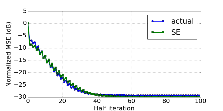
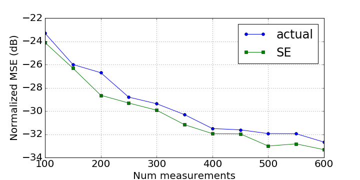
Figure 1: Simulation with a randomly generated neural network. Left panel: Normalized mean squared error (NMSE) for ML-VAMP and the predicted value from the state evolution as a function of the iteration with $M=300$ measurements. Right panel: Final NMSE for ML-VAMP and the SE prediction as a function of the measurements

The left panel of Fig. 1 shows the normalized mean squared error (NMSE) for the estimation of the inputs to the networks $\mathbf{z}_{0}$ as a function of the iteration number for a fixed number of measurements $M=300$. Also plotted is the state evolution (SE) prediction. We see that the SE predicts the ML-VAMP behavior remarkably well, within approximately 1 dB. The right panel shows the NMSE after 50 iterations (100 half-iterations) for various values of $M$. We again see an excellent agreement between the actual values and the SE predictions.

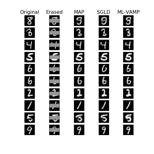
Figure 2: Inpainting of handwritten digits using MAP estimation, stochastic gradient Langevin dynamics (SGLD) and ML-VAMP.

MNIST inpainting

To demonstrate the feasibility of ML-VAMP on a real dataset, we used the algorithm for inpainting on the MNIST dataset, as considered in [4, 5, 41]. The MNIST dataset consists of 28 $\times$ 28 = 784 pixel images of hand-written digits as shown in the first column of Fig. 2. Following [2], a generative model for these digits was trained using a variational autoencoder (VAE), so that each image $\mathbf{x}$ is modeled as the output of an $L$-stage neural network. In this experiment, we used a single layer network with 20 input units, 400 hidden units and 784 output units corresponding to the dimension of the images – details of the network, training procedure and other simulation details are given in Appendix F. For each image $\mathbf{x}$, we then created an occluded image, $\mathbf{y}$, by removing the rows 10–20 of the image as shown in the second column of Fig. 2. The inpainting problem is to recover the original image $\mathbf{x}$ from the occluded image $\mathbf{y}$.

To perform ML-VAMP for reconstruction, we first observe that the occluded image $\mathbf{y}$ is the output of the same neural network that generates $\mathbf{x}$, but with the occuluded pixels removed in the final layer. Using the ML-VAMP algorithm, we can then estimate the values of $\mathbf{z}_{0}$, the input to the neural network. Once $\mathbf{z}_{0}$ is estimated, we can estimate the original image $\mathbf{x}$ by running the input $\mathbf{z}_{0}$ through the original network. The resulting reconstructed images are shown in the final column of Fig. 2, which displays the reconstructed images after only 20 iterations of ML-VAMP.

For comparison, we have also shown the MAP estimates, which are the images $\mathbf{x}$ that maximizes the posterior density $p(\mathbf{x}|\mathbf{y})$. As described in Appendix F, the MAP estimates can be computed using numerical optimization of the posterior density as performed in [4, 5]. Fig. 2 also shows the posterior mean $\mathbb{E}(\mathbf{x}|\mathbf{y})$ as estimated via Stochastic Gradient Langevin Dynamics (SGLD) [42] – also see Appendix F. We see that visually, the ML-VAMP, MAP and SGLD estimates are extremely similar.

In addition, the ML-VAMP algorithm is significantly faster: ML-VAMP was performed for only 20 iterations, while MAP used 500 iterations and SGLD used 10000. Thus, the experiment suggests that, in addition to its theoretical guarantees, ML-VAMP may also be a computationally simpler approach for reconstruction. Of course, much further experimentation on more complex data sets would be needed to evaluate its practical applicability.

V Conclusions

While deep networks have been remarkably successful in a range of challenging machine learning problems, their success is still not fully understood at a theoretical level. We have presented a principled and computationally tractable method for inference in deep networks whose performance can be rigorously characterized in certain high-dimensional random settings. The proposed method is based on AMP techniques which have proven to be information theoretically optimal in closely related problems. It is possible that similar optimality results may be true for ML-VAMP as well. For practical applications, the proposed method needs much further study, but its fast convergence suggests that it may be useful in problems outside the theoretical model as well. Going forward, the natural extension of these results would be to consider learning as well. AMP and VAMP techniques have been combined with EM learning in [43, 44, 45, 46] and it is possible that these methods may be able to be used in the context of learning deep generative models as well.

Appendix A Empirical Convergence of Vectors

We review some definitions from the Bayati-Montanari paper [40] and the original VAMP paper [29] since we will use the same analysis framework in this paper. Let $\mathbf{x}=(\mathbf{x}_{1},\ldots,\mathbf{x}_{N})$ be a block vector with components $\mathbf{x}_{n}\in{\mathbb{R}}^{r}$ for some $r$. Thus, the vector $\mathbf{x}$ is a vector with dimension $rN$. Given any function $g:{\mathbb{R}}^{r}\rightarrow{\mathbb{R}}^{s}$, we define the componentwise extension of $g(\cdot)$ as the function,

$$\mathbf{g}(\mathbf{x}):=(g(\mathbf{x}_{1}),\ldots,g(\mathbf{x}_{N}))\in{\mathbb{R}}^{Ns}.$$ (28)

That is, $\mathbf{g}(\cdot)$ applies the function $g(\cdot)$ on each $r$-dimensional component. Similarly, we say $\mathbf{g}(\mathbf{x})$ acts componentwise on $\mathbf{x}$ whenever it is of the form (28) for some function $g(\cdot)$.

Next consider a sequence of block vectors of growing dimension,

$$\mathbf{x}(N)=(\mathbf{x}_{1}(N),\ldots,\mathbf{x}_{N}(N)),\qquad N=1,\,2,\,\ldots,$$

where each component $\mathbf{x}_{n}(N)\in{\mathbb{R}}^{r}$. In this case, we will say that $\mathbf{x}(N)$ is a block vector sequence that scales with $N$ under blocks $\mathbf{x}_{n}(N)\in{\mathbb{R}}^{r}$. When $r=1$, so that the blocks are scalar, we will simply say that $\mathbf{x}(N)$ is a vector sequence that scales with $N$. Such vector sequences can be deterministic or random. In most cases, we will omit the notational dependence on $N$ and simply write $\mathbf{x}$.

Now, given $p\geq 1$, a function $f:{\mathbb{R}}^{r}\rightarrow{\mathbb{R}}^{s}$ is called pseudo-Lipschitz continuous of order $p$, if there exists a constant $C>0$ such that for all $\mathbf{x}_{1},\mathbf{x}_{2}\in{\mathbb{R}}^{r}$,

$$\|f(\mathbf{x}_{1})-f(\mathbf{x}_{2})\|\leq C\|\mathbf{x}_{1}-\mathbf{x}_{2}\|\left[1+\|\mathbf{x}_{1}\|^{p-1}+\|\mathbf{x}_{2}\|^{p-1}\right].$$

Observe that in the case $p=1$, pseudo-Lipschitz continuity reduces to the standard Lipschitz continuity. Given $p\geq 1$, we will say that the block vector sequence $\mathbf{x}=\mathbf{x}(N)$ converges empirically with $p$-th order moments if there exists a random variable $X\in{\mathbb{R}}^{r}$ such that

1. $\mathbb{E}\|X\|_{p}^{p}<\infty$; and

2. for any $f:{\mathbb{R}}^{r}\rightarrow{\mathbb{R}}$ that is pseudo-Lipschitz continuous of order $p$,

   $$\lim_{N\rightarrow\infty}\frac{1}{N}\sum_{n=1}^{N}f(\mathbf{x}_{n}(N))=\mathbb{E}\left[f(X)\right].$$ (29)

In (29), we have the empirical mean of the components $f(\mathbf{x}_{n}(N))$ of the componentwise extension $\mathbf{f}(\mathbf{x}(N))$ converging to the expectation $\mathbb{E}[f(X)]$. In this case, with some abuse of notation, we will write

$$\lim_{N\rightarrow\infty}\left\{\mathbf{x}_{n}\right\}\stackrel{{\scriptstyle PL(p)}}{{=}}X,$$ (30)

where, as usual, we have omitted the dependence on $N$ in $\mathbf{x}_{n}(N)$. Importantly, empirical convergence can de defined on deterministic vector sequences, with no need for a probability space. If $\mathbf{x}=\mathbf{x}(N)$ is a random vector sequence, we will often require that the limit (30) holds almost surely.

We conclude with one final definition. Let ${\bm{\phi}}(\mathbf{r},\gamma)$ be a function on $\mathbf{r}\in{\mathbb{R}}^{s}$ and $\gamma\in{\mathbb{R}}$. We say that ${\bm{\phi}}(\mathbf{r},\gamma)$ is uniformly Lipschitz continuous in $\mathbf{r}$ at $\gamma=\overline{\gamma}$ if there exists constants $L_{1}$ and $L_{2}\geq 0$ and an open neighborhood $U$ of $\overline{\gamma}$, such that

$$\|{\bm{\phi}}(\mathbf{r}_{1},\gamma)-{\bm{\phi}}(\mathbf{r}_{2},\gamma)\|\leq L_{1}\|\mathbf{r}_{1}-\mathbf{r}_{2}\|,$$ (31)

for all $\mathbf{r}_{1},\mathbf{r}_{2}\in{\mathbb{R}}^{s}$ and $\gamma\in U$; and

$$\|{\bm{\phi}}(\mathbf{r},\gamma_{1})-{\bm{\phi}}(\mathbf{r},\gamma_{2})\|\leq L_{2}\left(1+\|\mathbf{r}\|\right)|\gamma_{1}-\gamma_{2}|,$$ (32)

for all $\mathbf{r}\in{\mathbb{R}}^{s}$ and $\gamma_{1},\gamma_{2}\in U$.

Appendix B Linear Estimation Functions

Consider a linear factor node between two variables $\mathbf{z}_{\ell}$ and $\mathbf{z}_{\ell\!-\!1}$ related by the linear relation (1a), which corresponds to a Gaussian log conditional density,

$$-\ln p(\mathbf{z}_{\ell}|\mathbf{z}_{\ell\!-\!1})=\frac{\nu_{\ell}}{2}\|\mathbf{z}_{\ell}-\mathbf{W}_{\ell}\mathbf{z}_{\ell\!-\!1}+\mathbf{b}_{\ell}\|^{2}+\mbox{const}.$$ (33)

Applying (33), the energy function (4) is the quadratic

$$H(\mathbf{z}_{\ell\!-\!1},\mathbf{z}_{\ell}):=\frac{\nu_{\ell}}{2}\|\mathbf{z}_{\ell}-\mathbf{W}_{\ell}\mathbf{z}_{\ell\!-\!1}+\mathbf{b}_{\ell}\|^{2}+\frac{\gamma^{-}_{\ell}}{2}\|\mathbf{z}_{\ell}-\mathbf{r}^{-}_{\ell}\|^{2}+\frac{\gamma^{+}_{\ell\!-\!1}}{2}\|\mathbf{z}_{\ell\!-\!1}-\mathbf{r}^{-}_{\ell\!-\!1}\|^{2},$$ (34)

and the belief estimate $b(\cdot)$ in (3) is the Gaussian density

$$b(\mathbf{z}_{\ell\!-\!1},\mathbf{z}_{\ell}|\mathbf{r}_{\ell},\mathbf{r}_{\ell\!-\!1},\gamma_{\ell}^{-},\gamma_{\ell\!-\!1}^{+})\propto\exp\left[-H(\mathbf{z}_{\ell\!-\!1},\mathbf{z}_{\ell})\right].$$ (35)

As shown in (5), the estimation functions $\mathbf{g}^{\pm}_{\ell}(\cdot)$ are given by the expectation of $\mathbf{z}_{\ell\!-\!1}$ and $\mathbf{z}_{\ell}$ with respect to the density $b(\cdot)$ in (35). Since $b(\cdot)$ is Gaussian, these expectations can be computed via a least-squares problem.

The solution to this least-squares problem is simplest to consider using the SVD in (10). Specifically, given the SVD, define the transformed variables

$$\mathbf{u}_{\ell}:=\mathbf{V}_{\ell}^{\text{\sf T}}\mathbf{z}_{\ell},\quad\mathbf{u}_{\ell\!-\!1}:=\mathbf{V}_{\ell\!-\!1}\mathbf{z}_{\ell\!-\!1},\quad\bar{\mathbf{u}}_{\ell}:=\mathbf{V}_{\ell}^{\text{\sf T}}\mathbf{r}_{\ell}^{-},\quad\bar{\mathbf{u}}_{\ell\!-\!1}:=\mathbf{V}_{\ell\!-\!1}\mathbf{r}_{\ell\!-\!1}^{+},\quad\bar{\mathbf{b}}_{\ell}:=\mathbf{V}_{\ell}^{\text{\sf T}}\mathbf{b}_{\ell}.$$ (36)

To compute the expectations on $(\mathbf{z}_{\ell\!-\!1},\mathbf{z}_{\ell})$, we will first compute the expectations on $(\mathbf{u}_{\ell\!-\!1},\mathbf{u}_{\ell})$ and then use the transformations (36) to find the expectations on $(\mathbf{z}_{\ell\!-\!1},\mathbf{z}_{\ell})$. Using the transformations in (36), it can be verified that $\mathbf{u}=(\mathbf{u}_{\ell\!-\!1},\mathbf{u}_{\ell})$ has a Gaussian probability density,

$$b_{u}(\mathbf{u})\propto\exp\left[-H_{u}(\mathbf{u})\right],$$ (37)

where $H_{u}(\cdot)$ is the energy function

$$H_{u}(\mathbf{u}_{\ell\!-\!1},\mathbf{u}_{\ell})=\frac{\nu_{\ell}}{2}\|\mathbf{u}_{\ell}-{\bm{\Sigma}}_{\ell}\mathbf{u}_{\ell\!-\!1}+\bar{\mathbf{b}}_{\ell}\|^{2}+\frac{\gamma^{-}_{\ell}}{2}\|\mathbf{u}_{\ell}-\bar{\mathbf{u}}_{\ell}\|^{2}+\frac{\gamma^{+}_{\ell\!-\!1}}{2}\|\mathbf{u}_{\ell\!-\!1}-\bar{\mathbf{u}}_{\ell\!-\!1}\|^{2}.$$ (38)

This density has mean and covariance

$$\mathbb{E}(\mathbf{u}|b_{u})=\mathbf{Q}^{-1}\mathbf{c},\quad\mathrm{Cov}(\mathbf{u}|b_{u})=\mathbf{Q}^{-1},$$ (39)

where

$$\mathbf{Q}:=\left[\begin{array}[]{cc}\gamma_{\ell\!-\!1}^{+}\mathbf{I}+\nu_{\ell}{\bm{\Sigma}}_{\ell}^{\text{\sf T}}{\bm{\Sigma}}_{\ell}&-\nu_{\ell}{\bm{\Sigma}}_{\ell}^{\text{\sf T}}\\ -\nu_{\ell}{\bm{\Sigma}}_{\ell}&(\gamma_{\ell}^{-}+\nu_{\ell})\mathbf{I}\end{array}\right],\quad\mathbf{c}:=\left[\begin{array}[]{c}\gamma_{\ell\!-\!1}^{+}\bar{\mathbf{u}}_{\ell\!-\!1}-\nu_{\ell}{\bm{\Sigma}}_{\ell}^{\text{\sf T}}\bar{\mathbf{b}}_{\ell}\\ \gamma_{\ell}^{-}\bar{\mathbf{u}}_{\ell}+\nu_{\ell}\bar{\mathbf{b}}_{\ell}\end{array}\right].$$ (40)

To evaluate the expectation and covariance in (39), define the function $G_{\ell}(\cdot)$ with two outputs

$$G_{\ell}(\bar{u}_{\ell\!-\!1},\bar{u}_{\ell},s_{\ell},\bar{b}_{\ell},\gamma_{\ell\!-\!1}^{+},\gamma_{\ell}^{-}):=\left[\begin{array}[]{c}G_{\ell}^{-}(\bar{u}_{\ell\!-\!1},\bar{u}_{\ell},s_{\ell},\bar{b}_{\ell},\gamma_{\ell\!-\!1}^{+},\gamma_{\ell}^{-})\\ G_{\ell}^{+}(\bar{u}_{\ell\!-\!1},\bar{u}_{\ell},s_{\ell},\bar{b}_{\ell},\gamma_{\ell\!-\!1}^{+},\gamma_{\ell}^{-})\end{array}\right]=\mathbf{P}^{-1}\mathbf{d},$$ (41)

where $\mathbf{P}\in{\mathbb{R}}^{2\times 2}$ and $\mathbf{d}\in{\mathbb{R}}^{2\times 1}$ given by

$$\mathbf{P}:=\left[\begin{array}[]{cc}\gamma_{\ell\!-\!1}^{+}+\nu_{\ell}s_{\ell}^{2}&-\nu_{\ell}s_{\ell}\\ -\nu_{\ell}s_{\ell}&\gamma_{\ell}^{-}+\nu_{\ell}\end{array}\right],\quad\mathbf{d}:=\left[\begin{array}[]{c}\gamma_{\ell\!-\!1}^{+}\bar{u}_{\ell\!-\!1}-\nu_{\ell}s_{\ell}\bar{b}_{\ell}\\ \gamma_{\ell}^{-}\bar{u}_{\ell}+\nu_{\ell}\bar{b}_{\ell}\end{array}\right].$$ (42)

Since ${\bm{\Sigma}}_{\ell}$ has the block diagonal structure in (10), the expectations in (39) are given by

$$\mathbb{E}(\mathbf{u}_{\ell\!-\!1}|b_{u})=\mathbf{G}_{\ell}^{-}(\bar{\mathbf{u}}_{\ell\!-\!1},\bar{\mathbf{u}}_{\ell},\mathbf{s}_{\ell},\bar{\mathbf{b}}_{\ell},\gamma_{\ell\!-\!1}^{+},\gamma_{\ell}^{-}),$$ (43a)

$$\mathbb{E}(\mathbf{u}_{\ell}|b_{u})=\mathbf{G}_{\ell}^{+}(\bar{\mathbf{u}}_{\ell\!-\!1},\bar{\mathbf{u}}_{\ell},\mathbf{s}_{\ell},\bar{\mathbf{b}}_{\ell},\gamma_{\ell\!-\!1}^{+},\gamma_{\ell}^{-}),$$ (43b)

where the functions $\mathbf{G}_{\ell}^{\pm}(\cdot)$ are the componentwise extensions (see Appendix A) of $G_{\ell}^{\pm}(\cdot)$, meaning

$$\left[\mathbf{G}_{\ell}^{\pm}(\bar{\mathbf{u}}_{\ell\!-\!1},\bar{\mathbf{u}}_{\ell},\mathbf{s}_{\ell},\bar{\mathbf{b}}_{\ell},\gamma_{\ell\!-\!1}^{+},\gamma_{\ell}^{-})\right]_{n}=G_{\ell}^{\pm}(\bar{u}_{\ell\!-\!1,n},\bar{u}_{\ell n},s_{\ell n}\bar{b}_{\ell n},\gamma_{\ell\!-\!1}^{+},\gamma_{\ell}^{-}),$$ (44)

for each component $n$.

One slight technicality in the componentwise definition (44) is that $\bar{\mathbf{u}}_{\ell\!-\!1}$, $\bar{\mathbf{u}}_{\ell}$ and $\mathbf{s}_{\ell}$ may have different dimensions:

$$\bar{\mathbf{u}}_{\ell\!-\!1}\in{\mathbb{R}}^{N_{\ell\!-\!1}},\quad\bar{\mathbf{u}}_{\ell}\in{\mathbb{R}}^{N_{\ell}},\quad\mathbf{s}_{\ell}\in{\mathbb{R}}^{R_{\ell}}.$$

We define the outputs of $\mathbf{G}_{\ell}^{+}(\cdot)$ and $\mathbf{G}_{\ell}^{-}(\cdot)$ as having output dimensions $N_{\ell\!-\!1}$ and $N_{\ell}$, respectively. For $n\leq R_{\ell}$, we can use the formula (44) since $N_{\ell\!-\!1},N_{\ell}\geq R_{\ell}$ so all three terms $\bar{u}_{\ell\!-\!1,n},\bar{u}_{\ell n},s_{\ell n}$ are defined for $n\leq R_{\ell}$. For $n>R_{\ell}$, we use the convention that $s_{\ell n}=0$. In this case, it can be verified from (41) that when $s_{\ell n}=0$,

$$G_{\ell}^{-}(\bar{u}_{\ell\!-\!1,n},\bar{u}_{\ell n},s_{\ell n},\bar{b}_{\ell n},\gamma_{\ell\!-\!1}^{+},\gamma_{\ell}^{-}) =\bar{u}_{\ell\!-\!1},$$

$$G_{\ell}^{+}(\bar{u}_{\ell\!-\!1,n},\bar{u}_{\ell n},s_{\ell n},\bar{b}_{\ell n},\gamma_{\ell\!-\!1}^{+},\gamma_{\ell}^{-}) =\frac{\gamma_{\ell}^{-}\bar{u}_{\ell}+\nu_{\ell}\bar{b}_{\ell n}}{\gamma_{\ell}^{-}+\nu_{\ell}}.$$

Thus, $G_{\ell}^{-}(\cdot)$ does not depend on $\bar{u}_{\ell n}$ and $G_{\ell}^{+}(\cdot)$ does not depend on $\bar{u}_{\ell\!-\!1,n}$.

Using the definitions (36), we can compute the desired estimation functions

$$\mathbb{E}(\mathbf{z}_{\ell}|b)=\mathbf{V}_{\ell}\mathbb{E}(\mathbf{u}_{\ell}|b_{u})=\mathbf{V}_{\ell}\mathbf{G}_{\ell}^{+}(\bar{\mathbf{u}}_{\ell\!-\!1},\bar{\mathbf{u}}_{\ell},\mathbf{s},\mathbf{v},\gamma_{\ell\!-\!1}^{+},\gamma_{\ell}^{-})$$

$$=\mathbf{V}_{\ell}\mathbf{G}_{\ell}^{+}(\mathbf{V}_{\ell\!-\!1}\mathbf{r}^{+}_{\ell\!-\!1},\mathbf{V}_{\ell}^{\text{\sf T}}\mathbf{r}^{-}_{\ell},\mathbf{s}_{\ell},\bar{\mathbf{b}}_{\ell},\gamma_{\ell\!-\!1}^{+},\gamma_{\ell}^{-}).$$

Therefore, from (5), the linear estimation function is given by

$$\mathbf{g}^{+}_{\ell}(\mathbf{r}^{+}_{\ell\!-\!1},\mathbf{r}^{-}_{\ell},\gamma_{\ell\!-\!1}^{+},\gamma_{\ell}^{-})=\mathbf{V}_{\ell}\mathbf{G}_{\ell}^{+}(\mathbf{V}_{\ell\!-\!1}\mathbf{r}^{+}_{\ell\!-\!1},\mathbf{V}_{\ell}^{\text{\sf T}}\mathbf{r}^{-}_{\ell},\mathbf{s}_{\ell},\bar{\mathbf{b}}_{\ell},\gamma_{\ell\!-\!1}^{+},\gamma_{\ell}^{-}),$$ (45)

where we have suppressed the dependence on $\mathbf{s}_{\ell}$ and $\bar{\mathbf{b}}_{\ell}$ on the left hand side. Similarly, one can show

$$\mathbf{g}^{-}_{\ell}(\mathbf{r}^{+}_{\ell\!-\!1},\mathbf{r}^{-}_{\ell},\gamma_{\ell\!-\!1}^{+},\gamma_{\ell}^{-})=\mathbf{V}_{\ell\!-\!1}^{\text{\sf T}}\mathbf{G}_{\ell}^{-}(\mathbf{V}_{\ell\!-\!1}\mathbf{r}^{+}_{\ell\!-\!1},\mathbf{V}_{\ell}^{\text{\sf T}}\mathbf{r}^{-}_{\ell},\mathbf{s}_{\ell},\bar{\mathbf{b}}_{\ell},\gamma_{\ell\!-\!1}^{+},\gamma_{\ell}^{-}).$$ (46)

For the derivative $\alpha_{k\ell}$ in line 10, observe that

$$\alpha_{k\ell}^{+} \stackrel{{\scriptstyle(a)}}{{=}}{\langle\partial\mathbf{g}^{+}_{\ell}(\mathbf{r}^{+}_{k,\ell\!-\!1},\mathbf{r}^{-}_{k\ell},\mathbf{s}_{\ell},\gamma_{k\ell\!-\!1}^{+},\gamma_{k\ell}^{-})/\partial\mathbf{r}^{-}_{k\ell}\rangle}$$

$$\stackrel{{\scriptstyle(b)}}{{=}}\frac{1}{N_{\ell}}\mathrm{Tr}\left[\mathbf{V}_{\ell}\frac{\partial\mathbf{G}_{\ell}^{+}(\bar{\mathbf{u}}_{k,\ell\!-\!1},\bar{\mathbf{u}}_{\ell},\mathbf{s}_{\ell},\bar{\mathbf{b}}_{\ell},\gamma_{k,\ell\!-\!1}^{+},\gamma_{k\ell}^{-})}{\partial\bar{\mathbf{u}}_{k\ell}}\mathbf{V}_{\ell}^{\text{\sf T}}\right]$$

$$\stackrel{{\scriptstyle(c)}}{{=}}\frac{1}{N_{\ell}}\mathrm{Tr}\left[\frac{\partial\mathbf{G}_{\ell}^{+}(\bar{\mathbf{u}}_{k,\ell\!-\!1},\bar{\mathbf{u}}_{k\ell},\mathbf{s}_{\ell},\bar{\mathbf{b}}_{\ell},\gamma_{k,\ell\!-\!1}^{+},\gamma_{k\ell}^{-})}{\partial\bar{\mathbf{u}}_{k\ell}}\right]$$

$$\stackrel{{\scriptstyle(d)}}{{=}}{\left\langle\frac{\partial\mathbf{G}_{\ell}^{+}(\bar{\mathbf{u}}_{k,\ell\!-\!1},\bar{\mathbf{u}}_{k\ell},\mathbf{s}_{\ell},\bar{\mathbf{b}}_{\ell},\gamma_{k,\ell\!-\!1}^{+},\gamma_{k\ell}^{-})}{\partial\bar{\mathbf{u}}_{k\ell}}\right\rangle},$$ (47)

where (a) follows from line 10 of Algorithm 1; in (b), we have used (45) and set $\bar{\mathbf{u}}_{k,\ell\!-\!1}=\mathbf{V}_{\ell\!-\!1}\mathbf{r}^{+}_{k,\ell\!-\!1}$ and $\bar{\mathbf{u}}_{k\ell}=\mathbf{V}_{\ell}^{\text{\sf T}}\mathbf{r}^{+}_{k\ell}$; (c) follows from invariance of the trace of a product to cyclic permutation, since $\mathbf{V}_{\ell}^{\text{\sf T}}\mathbf{V}_{\ell}=\mathbf{I}$; and (d) follows from the definition of the ${\langle\cdot\rangle}$ operator. Similarly, we can show

$$\alpha_{k\ell}^{-}={\left\langle\frac{\partial\mathbf{G}_{\ell}^{-}(\bar{\mathbf{u}}_{k,\ell\!-\!1},\bar{\mathbf{u}}_{k\ell},\mathbf{s}_{\ell},\bar{\mathbf{b}}_{\ell},\gamma_{k,\ell\!-\!1}^{+},\gamma_{k\ell}^{-})}{\partial\bar{\mathbf{u}}_{k,\ell\!-\!1}}\right\rangle}.$$ (48)

Appendix C General Multi-Layer Recursions

To analyze Algorithm 1, we consider a more general class of recursions as shown in Algorithm 3. The Gen-ML Algorithm generates vectors $\mathbf{q}^{\pm}_{k\ell}$ and $\mathbf{p}^{\pm}_{k\ell}$ via a sequence of forward and backward passes through a multi-layer system. As we will show below, we will associate $\mathbf{q}^{\pm}_{k\ell}$ and $\mathbf{p}^{\pm}_{k\ell}$ with certain error terms in the ML-VAMP algorithm. The functions that update $\mathbf{f}_{k\ell}^{\pm}(\cdot)$ that produce the vectors $\mathbf{q}^{\pm}_{k\ell}$ and $\mathbf{p}^{\pm}_{k\ell}$ will be called the vector update functions.

To account for the effect of the parameters $\gamma^{\pm}_{k\ell}$ and $\alpha^{\pm}_{k\ell}$ in ML-VAMP, the Gen-ML algorithm describes the parameter update through a sequence of parameter lists $\Lambda^{\pm}_{k\ell}$. The parameter lists are ordered lists of parameters that accumulate as the algorithm progresses. They are initialized with $\Lambda^{-}_{01}$ in line 2. Then, as the algorithm progresses, new parameters $\lambda^{\pm}_{k\ell}$ are computed and then added to the lists in lines 12, 17, 24 and 29. The vector update functions $\mathbf{f}_{k\ell}^{\pm}(\cdot)$ may depend on any sets of parameters accumulated in the parameter list.

In lines 11, 16, 23 and 28, the new parameters $\lambda_{k\ell}^{\pm}$ are computed by: (1) computing average values $\mu_{k\ell}^{\pm}$ of componentwise functions ${\bm{\varphi}}^{\pm}_{k\ell}(\cdot)$; and (2) taking functions $T^{\pm}_{k\ell}(\cdot)$ of the average values $\mu_{k\ell}^{\pm}$. Since the average values $\mu_{k\ell}^{\pm}$ represent statistics on the components of ${\bm{\varphi}}^{\pm}_{k\ell}(\cdot)$, we will call ${\bm{\varphi}}^{\pm}_{k\ell}(\cdot)$ the parameter statistic functions. We will call the $T^{\pm}_{k\ell}(\cdot)$ the parameter update functions. We will show below that the updates for the parameters $\gamma^{\pm}_{k\ell}$ and $\alpha^{\pm}_{k\ell}$ can be written in this form.

Algorithm 3 General Multi-Layer Recursion (Gen-ML)

0:  Vector update functions $\mathbf{f}^{\pm}_{k\ell}(\cdot)$, parameter statistic functions ${\bm{\varphi}}^{\pm}_{k\ell}(\cdot)$, parameter update functions $T^{\pm}_{k\ell}(\cdot)$, orthogonal matrices $\mathbf{V}_{\ell}$, disturbance vectors $\mathbf{w}^{\pm}_{\ell}$.

1:  // Initialization

2:  Initialize parameter list $\Lambda_{01}^{-}$, and vectors $\mathbf{p}_{0}^{0}$ and $\mathbf{q}_{0\ell}^{-}$, $\ell=0,\ldots,L\!-\!1$

3:  $\mathbf{q}^{0}_{0}=\mathbf{f}^{0}_{0}(\mathbf{w}_{0}),\quad\mathbf{p}^{0}_{0}=\mathbf{V}_{0}\mathbf{q}^{0}_{0}$

4:  for $\ell=1,\ldots,L\!-\!1$ do

5:     $\mathbf{q}^{0}_{\ell}=\mathbf{f}^{0}_{\ell}(\mathbf{p}^{0}_{\ell\!-\!1},\mathbf{w}_{\ell},\Lambda_{01}^{-})$

6:     $\mathbf{p}^{0}_{\ell}=\mathbf{V}_{\ell}\mathbf{q}^{0}_{\ell}$

7:  end for

8:  

9:  for $k=0,1,\dots$ do

10:     // Forward Pass

11:     $\lambda^{+}_{k0}=T_{k0}^{+}(\mu^{+}_{k0},\Lambda_{0k}^{-}),\quad\mu^{+}_{k0}={\langle{\bm{\varphi}}_{k0}^{+}(\mathbf{q}_{k0}^{-},\mathbf{w}_{0},\Lambda_{0k}^{-})\rangle}$

12:     $\Lambda_{k0}^{+}=(\Lambda_{k1}^{-},\lambda^{+}_{k0})$

13:     $\mathbf{q}_{k0}^{+}=\mathbf{f}^{+}_{k0}(\mathbf{q}_{k0}^{-},\mathbf{w}_{0},\Lambda^{+}_{k0})$

14:     $\mathbf{p}_{k0}^{+}=\mathbf{V}_{0}\mathbf{q}_{k0}^{+}$

15:     for $\ell=1,\ldots,L-1$ do

16:        $\lambda^{+}_{k\ell}=T_{k\ell}^{+}(\mu^{+}_{k\ell},\Lambda_{k,\ell\!-\!1}^{+}),\quad\mu^{+}_{k\ell}={\langle{\bm{\varphi}}_{k\ell}^{+}(\mathbf{p}^{0}_{\ell\!-\!1},\mathbf{p}^{+}_{k,\ell\!-\!1},\mathbf{q}_{k\ell}^{-},\mathbf{w}_{\ell},\Lambda_{k,\ell\!-\!1}^{+})\rangle}$

17:        $\Lambda_{k\ell}^{+}=(\Lambda_{k,\ell\!-\!1}^{+},\lambda^{+}_{k\ell})$

18:        $\mathbf{q}_{k\ell}^{+}=\mathbf{f}^{+}_{k\ell}(\mathbf{p}^{0}_{\ell\!-\!1},\mathbf{p}^{+}_{k,\ell\!-\!1},\mathbf{q}_{k\ell}^{-},\mathbf{w}_{\ell},\Lambda^{+}_{k\ell})$

19:        $\mathbf{p}_{k\ell}^{+}=\mathbf{V}_{\ell}\mathbf{q}_{k\ell}^{+}$

20:     end for

21:     

22:     // Reverse Pass

23:     $\lambda^{-}_{k\!+\!1,L}=T_{kL}^{-}(\mu^{-}_{kL},\Lambda_{k,L\!-\!1}^{+}),\quad\mu^{-}_{kL}={\langle{\bm{\varphi}}_{kL}^{-}(\mathbf{p}_{k,L\!-\!1}^{+},\mathbf{w}_{L},\Lambda_{k,L\!-\!1}^{+})\rangle}$

24:     $\Lambda_{k\!+\!1,L}^{-}=(\Lambda_{k,L\!-\!1}^{+},\lambda^{+}_{k\!+\!1,L})$

25:     $\mathbf{p}_{k\!+\!1,L\!-\!1}^{-}=\mathbf{f}^{-}_{kL}(\mathbf{p}^{0}_{L\!-\!1},\mathbf{p}_{k,L\!-\!1}^{+},\mathbf{w}_{L},\Lambda^{-}_{k\!+\!1,L})$

26:     $\mathbf{q}_{k\!+\!1,L\!-\!1}^{-}=\mathbf{V}_{L\!-\!1}^{\text{\sf T}}\mathbf{p}_{k\!+\!1,L\!-\!1}$

27:     for $\ell=L\!-\!1,\ldots,1$ do

28:        $\lambda^{-}_{k\!+\!1,\ell}=T_{k\ell}^{-}(\mu^{-}_{k\ell},\Lambda_{k\!+\!1,\ell\!+\!1}^{-}),\quad\mu^{-}_{k\ell}={\langle{\bm{\varphi}}_{k\ell}^{-}(\mathbf{p}_{\ell\!-\!1}^{0},\mathbf{p}_{k,\ell\!-\!1}^{+},\mathbf{q}_{k\!+\!1,\ell}^{-},\mathbf{w}_{\ell},\Lambda_{k\!+\!1,\ell\!+\!1}^{+})\rangle}$

29:        $\Lambda_{k\!+\!1,\ell}^{-}=(\Lambda_{k\!+\!1,\ell\!+\!1}^{-},\lambda^{-}_{k\!+\!1,\ell})$

30:        $\mathbf{p}_{k\!+\!1,\ell\!-\!1}^{-}=\mathbf{f}^{-}_{k\ell}(\mathbf{p}_{\ell\!-\!1}^{0},\mathbf{p}^{+}_{k,\ell\!-\!1},\mathbf{q}_{k\!+\!1,\ell}^{-},\mathbf{w}_{\ell},\Lambda^{-}_{k\ell})$

31:        $\mathbf{q}_{k\!+\!1,\ell\!-\!1}^{-}=\mathbf{V}_{\ell\!-\!1}^{\text{\sf T}}\mathbf{p}_{k\!+\!1,\ell\!-\!1}^{-}$

32:     end for

33:  end for

Similar to our analysis of the ML-VAMP Algorithm, we consider the following large-system limit (LSL) analysis of Gen-ML. Specifically, we consider a sequence of runs of the recursions indexed by $N$. For each $N$, let $N_{\ell}=N_{\ell}(N)$ be the dimension of the signals $\mathbf{p}_{\ell}^{\pm}$ and $\mathbf{q}_{\ell}^{\pm}$ as we assume that $\lim_{N\rightarrow\infty}N_{\ell}/N$ is a constant so that $N_{\ell}$ scales linearly with $N$. We then make the following assumptions.

Assumption 1.

For the vectors in the Gen-ML Algorithm (Algorithm 3), we assume:

1. The components of the initial conditions $\mathbf{q}_{0\ell}^{-}$, and disturbance vectors $\mathbf{w}_{\ell}$ converge jointly empirically with limits,

   $$\lim_{N\rightarrow\infty}\{q_{0\ell,n}^{-}\}\stackrel{{\scriptstyle PL(2)}}{{=}}Q_{0\ell}^{-},\quad\lim_{N\rightarrow\infty}\{w_{\ell,n}\}\stackrel{{\scriptstyle PL(2)}}{{=}}W_{\ell},$$ (49)

   where $Q_{0\ell}^{-}$ and $W_{\ell}$ are random variables such that $(Q_{00}^{-},\cdots,Q^{-}_{0,L\!-\!1})$ is a jointly Gaussian random vector. Also, for $\ell=0,\ldots,L\!-\!1$, $W_{\ell}$ and $Q_{0\ell}^{-}$ are independent. We also assume that the initial parameter list converges almost surely as

   $$\lim_{N\rightarrow\infty}\Lambda_{01}^{-}=\overline{\Lambda}_{01}^{-},$$ (50)

   to some list $\overline{\Lambda}_{01}^{-}$. The limit (50) means means that every element in the list $\lambda\in\Lambda_{01}^{-}$ converges to a limit $\lambda\rightarrow\overline{\lambda}$ as $N\rightarrow\infty$ almost surely.

2. The matrices $\mathbf{V}_{\ell}$ are Haar distributed on the set of $N_{\ell}\times N_{\ell}$ orthogonal matrices and are independent from one another and from the vectors $\mathbf{p}^{0}_{0}$, $\mathbf{q}_{0\ell}^{-}$, disturbance vectors $\mathbf{w}_{\ell}$.

3. The vector update functions $\mathbf{f}_{k\ell}^{\pm}(\cdot)$ and parameter update functions ${\bm{\varphi}}_{k\ell}^{\pm}(\cdot)$ act componentwise. For example, in the forward pass, at each stage $\ell$, we assume that for each output component $n$,

   $$\left[\mathbf{f}^{+}_{k\ell}(\mathbf{p}^{0}_{\ell\!-\!1},\mathbf{p}^{+}_{k,\ell\!-\!1},\mathbf{q}_{k\ell}^{-},\mathbf{w}_{\ell},\Lambda^{+}_{k\ell})\right]_{n}=f^{+}_{k\ell}(p^{0}_{\ell\!-\!1,n},p^{+}_{k,\ell\!-\!1,n},q_{k\ell,n}^{-},w_{\ell,n},\Lambda^{+}_{k\ell})$$

   $$\left[{\bm{\varphi}}^{\pm}_{k\ell}(\mathbf{p}^{0}_{\ell\!-\!1},\mathbf{p}^{+}_{k,\ell\!-\!1},\mathbf{q}_{k\ell}^{-},\mathbf{w}_{\ell},\Lambda^{+}_{k\ell})\right]_{n}=\varphi^{+}_{k\ell}(p^{0}_{\ell\!-\!1,n},p^{+}_{k,\ell\!-\!1,n},q_{k\ell,n}^{-},w_{\ell,n},\Lambda^{+}_{k\ell}),$$

   for some scalar-valued functions $f^{+}_{k\ell}(\cdot)$ and $\varphi^{+}_{k\ell}(\cdot)$. Similar definitions apply in the reverse directions and for the initial update functions $f^{0}_{\ell}(\cdot)$. We will call $f^{\pm}_{k\ell}(\cdot)$ the vector update component functions and $\varphi^{\pm}_{k\ell}(\cdot)$ the parameter update component functions.

Algorithm 4 Gen-ML State Evolution

0:  Vector update component functions $f^{0}_{\ell}(\cdot)$ and $f^{\pm}_{k\ell}(\cdot)$, parameter statistic component functions $\varphi^{\pm}_{k\ell}(\cdot)$, parameter update functions $T^{\pm}_{k\ell}(\cdot)$

1:  

2:  // Initial pass

3:  Initial random variables: $W_{\ell}$, $Q_{0\ell}^{-}$, $\ell=0,\ldots,L\!-\!1$

4:  Initial parameter list limit: $\overline{\Lambda}_{01}^{-}$

5:  $Q^{0}_{0}=f^{0}_{0}(W_{0},\overline{\Lambda}_{01}^{-}),\quad P^{0}_{0}\sim{\mathcal{N}}(0,\tau^{0}_{0}),\quad\tau^{0}_{0}=\mathbb{E}(Q^{0}_{0})^{2}$

6:  for $\ell=1,\ldots,L\!-\!1$ do

7:     $Q^{0}_{\ell}=f^{0}_{\ell}(P^{0}_{\ell\!-\!1},W_{\ell},\overline{\Lambda}_{01}^{-})$,  $P^{0}_{\ell}={\mathcal{N}}(0,\tau^{0}_{\ell})$,  $\tau^{0}_{\ell}=\mathbb{E}(Q^{0}_{\ell})^{2}$

8:  end for

9:  

10:  for $k=0,1,\dots$ do

11:     // Forward Pass

12:     $\overline{\lambda}^{+}_{k0}=T_{k0}^{+}(\overline{\mu}^{+}_{k0},\overline{\Lambda}_{0k}^{-}),\quad\overline{\mu}^{+}_{k0}=\mathbb{E}(\varphi_{k0}^{+}(Q_{k0}^{-},W_{0},\overline{\Lambda}_{0k}^{-}))$

13:     $\overline{\Lambda}_{k0}^{+}=(\overline{\Lambda}_{k1}^{-},\overline{\lambda}^{+}_{k0})$

14:     $Q_{k0}^{+}=f^{+}_{k0}(Q_{k0}^{-},W_{0},\overline{\Lambda}^{+}_{k0})$

15:     $(P^{0}_{0},P_{k0}^{+})={\mathcal{N}}(\mathbf{0},\mathbf{K}_{k0}^{+}),\quad\mathbf{K}_{k0}^{+}=\mathrm{Cov}(Q^{0}_{0},Q_{k0}^{+})$

16:     for $\ell=1,\ldots,L-1$ do

17:        $\overline{\lambda}^{+}_{k\ell}=T_{k\ell}^{+}(\overline{\mu}^{+}_{k\ell},\overline{\Lambda}_{k,\ell\!-\!1}^{+}),\quad\overline{\mu}^{+}_{k\ell}=\mathbb{E}(\varphi_{k\ell}^{+}(P^{0}_{\ell\!-\!1},P^{+}_{k,\ell\!-\!1},Q_{k\ell}^{-},W_{\ell},\overline{\Lambda}_{k,\ell\!-\!1}^{+}))$

18:        $\overline{\Lambda}_{k\ell}^{+}=(\overline{\Lambda}_{k,\ell\!-\!1}^{+},\overline{\lambda}^{+}_{k\ell})$

19:        $Q_{k\ell}^{+}=f^{+}_{k\ell}(P^{0}_{\ell\!-\!1},P^{+}_{k,\ell\!-\!1},Q_{k\ell}^{-},W_{\ell},\overline{\Lambda}^{+}_{k\ell})$

20:        $(P^{0}_{\ell},P_{k\ell}^{+})={\mathcal{N}}(\mathbf{0},\mathbf{K}_{k\ell}^{+}),\quad\mathbf{K}_{k\ell}^{+}=\mathrm{Cov}(Q^{0}_{\ell},Q_{k\ell}^{+})$

21:     end for

22:     

23:     // Reverse Pass

24:     $\overline{\lambda}^{-}_{k\!+\!1,L}=T_{kL}^{-}(\overline{\mu}^{-}_{kL},\overline{\Lambda}_{k,L\!-\!1}^{+}),\quad\overline{\mu}^{-}_{kL}=\mathbb{E}(\varphi_{kL}^{-}(P^{0}_{L\!-\!1},P_{k,L\!-\!1}^{+},W_{L},\overline{\Lambda}_{k,L\!-\!1}^{+}))$

25:     $\overline{\Lambda}_{k\!+\!1,L}^{-}=(\overline{\Lambda}_{k,L\!-\!1}^{+},\overline{\lambda}^{+}_{k\!+\!1,L})$

26:     $P_{k\!+\!1,L\!-\!1}^{-}=f^{-}_{kL}(P^{0}_{L\!-\!1},P_{k,L\!-\!1}^{+},W_{L},\overline{\Lambda}^{-}_{k\!+\!1,L})$

27:     $Q_{k\!+\!1,L\!-\!1}^{-}={\mathcal{N}}(0,\tau_{k\!+\!1,L\!-\!1}^{-}),\quad\tau_{k\!+\!1,L\!-\!1}^{-}=\mathbb{E}(P^{-}_{k\!+\!1,L\!-\!1})^{2}$

28:     for $\ell=L\!-\!1,\ldots,1$ do

29:        $\overline{\lambda}^{-}_{k\!+\!1,\ell}=T_{k\ell}^{-}(\overline{\mu}^{-}_{k\ell},\overline{\Lambda}_{k\!+\!1,\ell\!+\!1}^{-}),\quad\overline{\mu}^{-}_{k\ell}=\mathbb{E}(\varphi_{k\ell}^{-}(P^{0}_{\ell\!-\!1},P_{k,\ell\!-\!1}^{+},Q_{k\!+\!1,\ell}^{-},W_{\ell},\overline{\Lambda}_{k\!+\!1,\ell\!+\!1}^{+}))$

30:        $\overline{\Lambda}_{k\!+\!1,\ell}^{-}=(\overline{\Lambda}_{k\!+\!1,\ell\!+\!1}^{-},\overline{\lambda}^{-}_{k\!+\!1,\ell})$

31:        $P_{k\!+\!1,\ell\!-\!1}^{-}=f^{-}_{k\ell}(P^{0}_{\ell\!-\!1},P^{+}_{k,\ell\!-\!1},Q_{k\!+\!1,\ell}^{-},W_{\ell},\overline{\Lambda}^{-}_{k\ell})$

32:        $Q_{k\!+\!1,\ell\!-\!1}^{-}={\mathcal{N}}(0,\tau_{k\!+\!1,\ell\!-\!1}^{-}),\quad\tau_{k\!+\!1,\ell\!-\!1}^{-}=\mathbb{E}(P_{k\!+\!1,\ell\!-\!1}^{-})^{2}$

33:     end for

34:  end for

Under these assumptions, we iteratively define a sequences of constants and random variables through the recursions in Algorithm 4, which we call the Gen-ML state evolution. The SE recursions in Algorithm 4 closely mirrors those in the Gen-ML algorithm (Algorithm 3). The random vectors $\mathbf{q}^{\pm}_{k\ell}$ and $\mathbf{p}^{\pm}_{k\ell}$ are replaced by scalar random variables $Q^{\pm}_{k\ell}$ and $P^{\pm}_{k\ell}$; the vector and parameter update functions $\mathbf{f}^{+}_{k\ell}(\cdot)$ and ${\bm{\varphi}}^{+}_{k\ell}(\cdot)$ are replaced by their component functions $f^{+}_{k\ell}(\cdot)$ and $\varphi^{+}_{k\ell}(\cdot)$; and the parameters $\lambda_{k\ell}^{\pm}$ are replaced by their limits $\overline{\lambda}_{k\ell}^{\pm}$.

The various random variables, expectations and covariances in Algorithm 4 are computed as follows: In the initial pass, in line 7, we treat $P^{0}_{\ell\!-\!1}\sim{\mathcal{N}}(0,\tau^{0}_{\ell\!-\!1})$ and $W_{\ell}$ as independent for defining the random variable $Q^{0}_{\ell}$. In the forward pass, in lines  12 and 14, we treat $Q_{k0}^{-}$ and $W_{0}$ as independent. Then, in lines  17 and 19, we treat

$$(P^{0}_{\ell\!-\!1},P_{k,\ell\!-\!1}^{+})\sim{\mathcal{N}}(\mathbf{0},\mathbf{K}_{k,\ell\!-\!1}^{+}),\quad Q^{-}_{k\ell},\quad W_{\ell}$$

as independent. Similar independence assumptions are made in the reverse pass. We next make the following assumptions.

Assumption 2.

In addition to Assumption 1 assume:

1. The functions $T^{\pm}_{k\ell}(\mu_{k\ell}^{\pm},\cdot)$ are continuous at $\mu_{k\ell}^{\pm}=\overline{\mu}_{k\ell}^{\pm}$ where $\overline{\mu}_{k\ell}^{\pm}$ is the output of Algorithm 4.

2. The vector update component functions in the forward direction and their derivatives,

   $$f^{+}_{k\ell}(p^{+}_{k,\ell\!-\!1},q_{k\ell}^{-},w_{\ell},\Lambda^{+}_{k\ell}),\quad\partial f^{+}_{k\ell}(p^{+}_{k,\ell\!-\!1},q_{k\ell}^{-},w_{\ell},\Lambda^{+}_{k\ell})/\partial q_{k\ell}^{-},$$

   are uniformly Lipschitz continuous in $(p^{+}_{k,\ell\!-\!1},q_{k\ell}^{-},w_{\ell})$ at $\Lambda^{+}_{k\ell}=\overline{\Lambda}^{+}_{k\ell}$. Similarly, in the reverse direction,

   $$f^{-}_{k\ell}(p^{+}_{k,\ell\!-\!1},q_{k\!+\!1,\ell}^{-},w_{\ell},\Lambda^{-}_{k\!+\!1,\ell}),\quad\partial f^{+}_{k\ell}(p^{+}_{k,\ell\!-\!1},q_{k\!+\!1,\ell}^{-},w_{\ell},\Lambda^{-}_{k\!+\!1,\ell})/\partial p_{k,\ell\!-\!1}^{+},$$

   are uniformly Lipschitz continuous in $(p^{+}_{k,\ell\!-\!1},q_{k\ell}^{-},w_{\ell})$ at $\Lambda^{-}_{k\!+\!1,\ell}=\overline{\Lambda}^{-}_{k\!+\!1,\ell}$. Also, the initial vector update component functions $f^{0}_{\ell}(p^{0}_{k,\ell\!-\!1},w_{\ell},\Lambda^{-}_{01})$ are uniformly Lipschitz continuous in $(p^{0}_{k,\ell\!-\!1},w_{\ell})$ at $\Lambda^{-}_{k\!+\!1,\ell}=\overline{\Lambda}^{-}_{k\!+\!1,\ell}$.

3. The vector update functions are asymptotically divergence free meaning

   $$\lim_{N\rightarrow\infty}{\langle\frac{\partial\mathbf{f}^{+}_{k\ell}(\mathbf{p}^{+}_{k,\ell\!-\!1},\mathbf{q}_{k\ell}^{-},\mathbf{w}_{\ell},\overline{\Lambda}^{+}_{k\ell})}{\partial\mathbf{q}_{k\ell}^{-}}\rangle}=0,\quad\lim_{N\rightarrow\infty}{\langle\frac{\partial\mathbf{f}^{-}_{k\ell}(\mathbf{p}^{+}_{k,\ell\!-\!1},\mathbf{q}_{k\ell}^{-},\mathbf{w}_{\ell},\overline{\Lambda}^{-}_{k\ell})}{\partial\mathbf{p}_{k,\ell\!-\!1}^{+}}\rangle}=0\\$$ (51)

4. The parameter update component functions in the forward direction $\varphi^{+}_{k\ell}(p^{+}_{k,\ell\!-\!1},q_{k\ell}^{-},w_{\ell},\Lambda^{+}_{k,\ell\!-\!1})$ are uniformly Lipschitz continuous in $(p^{+}_{k,\ell\!-\!1},q_{k\ell}^{-},w_{\ell})$ at $\Lambda^{+}_{k,\ell\!-\!1}=\overline{\Lambda}^{+}_{k,\ell\!-\!1}$. Analogous conditions apply to the reverse functions $\varphi^{-}_{k\ell}(\cdot)$

Under the above assumptions, the following theorem proves the SE equations for the Gen-ML recursion.

Theorem 2.

Consider the outputs of the Gen-ML recursion (Algorithm 3) and the corresponding random variables and parameter limits defined by the SE updates in Algorithm 4 under Assumptions 3 and 2. Then,

1. For any fixed $k$ and $\ell=1,\ldots,L\!-\!1$, the parameter list $\Lambda_{k\ell}^{+}$ converges as

   $$\lim_{N\rightarrow\infty}\Lambda_{k\ell}^{+}=\overline{\Lambda}_{k\ell}^{+}$$ (52)

   almost surely. Also, the components of $\mathbf{w}_{\ell}$, $\mathbf{p}^{0}_{\ell\!-\!1}$, $\mathbf{q}^{0}_{\ell}$, $\mathbf{p}_{0,\ell\!-\!1}^{+},\ldots,\mathbf{p}_{k,\ell\!-\!1}^{+}$ and $\mathbf{q}_{0\ell}^{\pm},\ldots,\mathbf{q}_{k\ell}^{\pm}$ almost surely empirically converge jointly with limits,

   $$\lim_{N\rightarrow\infty}\left\{(p^{0}_{\ell\!-\!1,n},p^{+}_{i,\ell\!-\!1,n},q^{0}_{\ell,n},q^{-}_{j\ell,n},q^{+}_{j\ell,n})\right\}=(P^{0}_{\ell\!-\!1},P^{+}_{i,\ell\!-\!1},Q^{0}_{\ell},Q^{-}_{j\ell},Q^{+}_{j\ell}),$$ (53)

   for all $i,j=0,\ldots,k$, where the variables $P^{0}_{\ell\!-\!1}$, $P_{i,\ell\!-\!1}^{+}$ and $Q_{j\ell}^{-}$ are zero-mean jointly Gaussian random variables independent of $W_{\ell}$ with

   $$\mathrm{Cov}(P^{0}_{\ell\!-\!1},P_{i,\ell\!-\!1}^{+})=\mathbf{K}_{i,\ell\!-\!1}^{+},\quad\mathbb{E}(Q_{j\ell}^{-})^{2}=\tau_{j\ell}^{-},\quad\mathbb{E}(P_{i,\ell\!-\!1}^{+}Q_{j\ell}^{-})=0,\quad\mathbb{E}(P^{0}_{\ell\!-\!1}Q_{j\ell}^{-})=0,$$ (54)

   and $Q^{0}_{\ell}$ and $Q^{+}_{j\ell}$ are the random variable in line 19:

   $$Q^{0}_{\ell}=f^{0}_{\ell}(P^{0}_{\ell\!-\!1},W_{\ell}),\quad Q^{+}_{j\ell}=f^{+}_{j\ell}(P^{0}_{\ell\!-\!1},P^{+}_{i,\ell\!-\!1},Q^{-}_{j\ell},W_{\ell},\overline{\Lambda}_{k\ell}^{+}).$$ (55)

   The identical result holds for $\ell=0$ with all the variables $\mathbf{p}_{i,\ell\!-\!1}^{+}$ and $P_{i,\ell\!-\!1}^{+}$ removed.

2. For any fixed $k>0$ and $\ell=1,\ldots,L\!-\!1$, the parameter lists $\Lambda_{k\ell}^{-}$ converge as

   $$\lim_{N\rightarrow\infty}\Lambda_{k\ell}^{-}=\overline{\Lambda}_{k\ell}^{-}$$ (56)

   almost surely. Also, the components of $\mathbf{w}_{\ell}$, $\mathbf{p}^{0}_{\ell\!-\!1}$, $\mathbf{p}_{0,\ell\!-\!1}^{+},\ldots,\mathbf{p}_{k\!-\!1,\ell\!-\!1}^{+}$, $\mathbf{p}_{0,\ell\!-\!1}^{+},\ldots,\mathbf{p}_{k\!-\!1,\ell\!-\!1}^{+}$, and $\mathbf{q}_{0\ell}^{-},\ldots,\mathbf{q}_{k\ell}^{-}$ almost surely empirically converge jointly with limits,

   $$\lim_{N\rightarrow\infty}\left\{(p^{0}_{\ell\!-\!1,n},p^{+}_{i,\ell\!-\!1,n},q^{-}_{j\ell,n},q^{+}_{j\ell,n})\right\}=(P^{0}_{\ell\!-\!1},P^{+}_{i,\ell\!-\!1},Q^{-}_{j\ell},Q^{+}_{j\ell}),$$ (57)

   for all $i=0,\ldots,k\!-\!1$ and $j=0,\ldots,k$, where the variables $P^{0}_{\ell\!-\!1}$, $P_{i,\ell\!-\!1}^{+}$ and $Q_{j\ell}^{-}$ are zero-mean jointly Gaussian random variables independent of $W_{\ell}$ with

   $$\mathrm{Cov}(P^{0}_{\ell\!-\!1},P_{i,\ell\!-\!1}^{+})=\mathbf{K}_{i,\ell\!-\!1}^{+},\quad\quad\mathbb{E}(Q_{j\ell}^{-})^{2}=\tau_{j\ell}^{-},\quad\mathbb{E}(P_{i,\ell\!-\!1}^{+}Q_{j\ell}^{-})=0,\quad\mathbb{E}(P^{0}_{\ell\!-\!1}Q_{j\ell}^{-})=0,$$ (58)

   and $P^{-}_{j\ell}$ is the random variable in line 31:

   $$P^{-}_{j\ell}=f^{-}_{j\ell}(P^{0}_{\ell\!-\!1},P^{+}_{i,\ell\!-\!1},Q^{-}_{j\ell},W_{\ell},\overline{\Lambda}_{k\ell}^{-}).$$ (59)

   The identical result holds for $\ell=L$ with all the variables $\mathbf{q}_{j\ell}^{-}$ and $Q_{j\ell}^{-}$ removed. Also, for $k=0$, we remove the variables with $\mathbf{p}_{k\!-\!1,\ell}^{+}$ and $P_{k\!-\!1,\ell}^{+}$.

Proof.

We will prove this in Appendix D. $\Box$

Appendix D Proof of Theorem 2

D-A Overview of the Induction Sequence

The proof is similar to that of [29, Theorem 4], which provides a SE analysis for VAMP on a single-layer network. The critical challenge here is to extend that proof to multi-layer recursions. Many of the ideas in the two proofs are similar, so we highlight only the key differences between the two.

Similar to the SE analysis of VAMP in [29], we use an induction argument. However, for the multi-layer proof, we must index over both the iteration index $k$ and layer index $\ell$. To this end, let $\mathcal{H}_{k\ell}^{+}$ and $\mathcal{H}_{k\ell}^{-}$ be the hypotheses:

• $\mathcal{H}_{k\ell}^{+}$: The hypothesis that Theorem 2(a) is true for some $k$ and $\ell$.

• $\mathcal{H}_{k\ell}^{-}$: The hypothesis that Theorem 2(b) is true for some $k$ and $\ell$.

We prove these hypotheses by induction via a sequence of implications,

$$\cdots\Rightarrow\mathcal{H}_{k1}^{-}\Rightarrow\mathcal{H}_{k0}^{+}\Rightarrow\cdots\Rightarrow\mathcal{H}_{k,L\!-\!1}^{+}\Rightarrow\mathcal{H}_{k\!+\!1,L}^{-}\Rightarrow\cdots\Rightarrow\mathcal{H}_{k1}^{-}\Rightarrow\cdots,$$ (60)

beginning with the hypothesis $\mathcal{H}^{-}_{0\ell}$ for all $\ell=1,\ldots,L\!-\!1$.

D-B Proof of the Induction Update

Now fix a stage index $\ell=1,\ldots,L\!-\!1$ and an iteration index $k=0,1,\ldots$. Assume, as an induction hypothesis, that all the hypotheses prior to $\mathcal{H}^{+}_{k,\ell\!+\!1}$ in the sequence (60) but not including $\mathcal{H}^{+}_{k,\ell\!+\!1}$ are true. We show that, under this assumption, $\mathcal{H}^{+}_{k,\ell\!+\!1}$ is true. The other implications in the hypothesis sequence (60) can be proven similarly.

We introduce with some notation. Let

$$\mathbf{P}_{k\ell}^{+}:=\left[\mathbf{p}_{0\ell}^{+}\cdots\mathbf{p}_{k\ell}^{+}\right]\in{\mathbb{R}}^{N_{\ell}\times(k\!+\!1)},$$

which is the matrix whose columns are the first $k\!+\!1$ values of the vector $\mathbf{p}^{+}_{i\ell}$. We define the matrices $\mathbf{P}_{k\ell}^{-}$, $\mathbf{Q}_{k\ell}^{+}$ and $\mathbf{Q}_{k\ell}^{-}$ similarly. Let $\mathfrak{G}_{k\ell}^{\pm}$ denote the collection of random variables associated with the hypotheses, $\mathcal{H}^{\pm}_{k\ell}$. That is, for $\ell=1,\ldots,L\!-\!1$,

$$\mathfrak{G}_{k\ell}^{+}:=\left\{\mathbf{w}_{\ell},\mathbf{p}^{0}_{\ell\!-\!1},\mathbf{P}^{+}_{k,\ell\!-\!1},\mathbf{q}^{0}_{\ell},\mathbf{Q}^{-}_{k\ell},\mathbf{Q}_{k\ell}^{+}\right\},\quad\mathfrak{G}_{k\ell}^{-}:=\left\{\mathbf{w}_{\ell},\mathbf{p}^{0}_{\ell\!-\!1},\mathbf{P}^{+}_{k\!-\!1,\ell\!-\!1},\mathbf{q}^{0}_{\ell},\mathbf{Q}^{-}_{k\ell},\mathbf{P}^{-}_{k,\ell\!-\!1}\right\}.$$ (61)

For $\ell=0$ and $\ell=L$ we set,

$$\mathfrak{G}_{k0}^{+}:=\left\{\mathbf{w}_{0},\mathbf{Q}^{-}_{k0},\mathbf{Q}_{k0}^{+}\right\},\quad\mathfrak{G}_{kL}^{-}:=\left\{\mathbf{w}_{L},\mathbf{p}^{0}_{L\!-\!1},\mathbf{P}^{+}_{k\!-\!1,L\!-\!1},\mathbf{P}^{-}_{k,L\!-\!1}\right\}.$$ (62)

With some abuse of notation, we let $\mathfrak{G}_{km\ell}$ also denote the sigma-algebra generated by these vectors. Also, let $\overline{\mathfrak{G}}_{k\ell}^{+}$ be the union of all the sets $\mathfrak{G}_{i\ell^{\prime}}^{\pm}$ as they appear in the sequence (60) up to and including the final set $\overline{\mathfrak{G}}_{k\ell}^{+}$. Thus, the set $\overline{\mathfrak{G}}_{k\ell}^{+}$ contains all the vectors produced by Algorithm 3 immediately before line 19 in stage $\ell$ of iteration $k$.

Now, the actions of the matrix $\mathbf{V}_{\ell}$ in Algorithm 3 are through the matrix-vector multiplications in lines 19 and 30. Hence, if we define the matrices,

$$\mathbf{A}_{k\ell}:=\left[\mathbf{p}^{0}_{\ell},\mathbf{P}_{k\!-\!1,\ell}^{+}~{}\mathbf{P}_{k\ell}^{-}\right],\quad\mathbf{B}_{k\ell}:=\left[\mathbf{q}^{0}_{\ell},\mathbf{Q}_{k\!-\!1,\ell}^{+}~{}\mathbf{Q}_{k\ell}^{-}\right],$$ (63)

all the vectors in the set $\overline{\mathfrak{G}}_{k\ell}^{+}$ will be unchanged for all matrices $\mathbf{V}_{\ell}$ satisfying the linear constraints

$$\mathbf{A}_{k\ell}=\mathbf{V}_{\ell}\mathbf{B}_{k\ell}.$$ (64)

Hence, the conditional distribution of $\mathbf{V}_{\ell}$ given $\overline{\mathfrak{G}}_{k\ell}^{+}$ is precisely the uniform distribution on the set of orthogonal matrices satisfying (64). The matrices $\mathbf{A}_{k\ell}$ and $\mathbf{B}_{k\ell}$ are of dimensions $N_{\ell}\times s$ where $s=2k+2$. From [29], this conditional distribution is given by

$$\left.\mathbf{V}_{\ell}\right|_{\overline{\mathfrak{G}}_{k\ell}^{+}}\stackrel{{\scriptstyle d}}{{=}}\mathbf{A}_{k\ell}(\mathbf{A}^{\text{\sf T}}_{k\ell}\mathbf{A}_{k\ell})^{-1}\mathbf{B}_{k\ell}^{\text{\sf T}}+\mathbf{U}_{\mathbf{A}_{k\ell}^{\perp}}\widetilde{\mathbf{V}}_{\ell}\mathbf{U}_{\mathbf{B}_{k\ell}^{\perp}}^{\text{\sf T}},$$ (65)

where $\mathbf{U}_{\mathbf{A}_{k\ell}^{\perp}}$ and $\mathbf{U}_{\mathbf{B}_{k\ell}^{\perp}}$ are $N\times(N-s)$ matrices whose columns are an orthonormal basis for $\mathrm{Range}(\mathbf{A}_{k\ell})^{\perp}$ and $\mathrm{Range}(\mathbf{B}_{k\ell})^{\perp}$. The matrix $\widetilde{\mathbf{V}}_{\ell}$ is Haar distributed on the set of $(N-s)\times(N-s)$ orthogonal matrices and independent of $\overline{\mathfrak{G}}_{k\ell}^{+}$.

Next, similar to the proof of [29, Theorem 4], we use (65) and write $\mathbf{p}_{k\ell}^{+}$ from line 19 as a sum of two terms

$$\mathbf{p}_{k\ell}^{+}=\mathbf{V}_{\ell}\mathbf{q}_{k\ell}^{+}=\mathbf{p}_{k\ell}^{\rm det}+\mathbf{p}_{k\ell}^{\rm ran},$$ (66)

where $\mathbf{p}_{k\ell}^{\rm+det}$ is what we will call the deterministic part:

$$\mathbf{p}_{k\ell}^{\rm det}=\mathbf{A}_{k\ell}(\mathbf{B}^{\text{\sf T}}_{k\ell}\mathbf{B}_{k\ell})^{-1}\mathbf{B}_{k\ell}^{\text{\sf T}}\mathbf{q}_{k\ell}^{+}$$ (67)

and $\mathbf{p}_{k\ell}^{\rm ran}$ is what we will call the random part:

$$\mathbf{p}_{k}^{\rm ran}=\mathbf{U}_{\mathbf{B}_{k}^{\perp}}\widetilde{\mathbf{V}}_{\ell}^{\text{\sf T}}\mathbf{U}_{\mathbf{A}_{k}^{\perp}}^{\text{\sf T}}\mathbf{q}_{k\ell}^{+}.$$ (68)

The next two lemmas characterize the limiting distributions of the deterministic and random components.

Lemma 1.

Under the induction hypothesis, the components of the “deterministic" component $\mathbf{p}_{k\ell}^{\rm det}$ along with the components of the vectors in $\overline{\mathfrak{G}}_{k\ell}^{+}$ converge empirically. In addition, there exists constants $\beta_{0\ell}^{+},\ldots,\beta^{+}_{k\!-\!1,\ell}$ such that

$$\lim_{N\rightarrow\infty}\{p_{k\ell,n}^{\rm det}\}\stackrel{{\scriptstyle PL(2)}}{{=}}P_{k\ell}^{\rm det}=\beta^{0}_{\ell}P^{0}_{\ell}+\sum_{i=0}^{k\!-\!1}\beta_{i\ell}P_{i\ell}^{+},$$ (69)

where $P_{k\ell}^{\rm det}$ is the limiting random variable for the components of $\mathbf{p}_{k\ell}^{\rm det}$.

Proof.

The proof is similar to the proof of [29, Lemma 6], but we will go over the details as there are some important differences in the multi-layer case. Define

$$\widetilde{\mathbf{P}}_{k\!-\!1,\ell}^{+}=\left[\mathbf{p}^{0}_{\ell},~{}\mathbf{P}_{k\!-\!1,\ell}^{+}\right],\quad\widetilde{\mathbf{Q}}_{k\!-\!1,\ell}^{+}=\left[\mathbf{q}^{0}_{\ell},~{}\mathbf{Q}_{k\!-\!1,\ell}^{+}\right],$$ (70)

which are the matrices $\mathbf{P}_{k\!-\!1,\ell}^{+}$ and $\mathbf{Q}_{k\!-\!1,\ell}^{+}$ with the additions of the columns $\mathbf{p}^{0}_{\ell}$ and $\mathbf{q}^{0}_{\ell}$. We can then write $\mathbf{A}_{k\ell}$ and $\mathbf{B}_{k\ell}$ in (63) as

$$\mathbf{A}_{k\ell}:=\left[\widetilde{\mathbf{P}}_{k\!-\!1,\ell}^{+}~{}\mathbf{P}_{k\ell}^{-}\right],\quad\mathbf{B}_{k\ell}:=\left[\widetilde{\mathbf{Q}}_{k\!-\!1,\ell}^{+}~{}\mathbf{Q}_{k\ell}^{-}\right],$$ (71)

We first evaluate the asymptotic values of various terms in (67). Using the definition of $\mathbf{A}_{k\ell}$ in (63),

$$\mathbf{B}^{\text{\sf T}}_{k\ell}\mathbf{B}_{k\ell}=\left[\begin{array}[]{cc}(\widetilde{\mathbf{Q}}_{k\!-\!1,\ell}^{+})^{\text{\sf T}}\widetilde{\mathbf{Q}}_{k\!-\!1,\ell}^{+}&(\widetilde{\mathbf{Q}}_{k\!-\!1,\ell}^{+})^{\text{\sf T}}\mathbf{Q}_{k\ell}^{-}\\ (\mathbf{Q}_{k\ell}^{-})^{\text{\sf T}}\widetilde{\mathbf{Q}}_{k\!-\!1,\ell}^{+}&(\mathbf{Q}_{k\ell}^{-})^{\text{\sf T}}\mathbf{Q}_{k\ell}^{-}\end{array}\right]$$

We can then easily evaluate the asymptotic value of these terms as follows: The asymptotic value of the $(i+1,j+1)$-th component of the matrix $(\widetilde{\mathbf{Q}}_{k\!-\!1,\ell}^{+})^{\text{\sf T}}\widetilde{\mathbf{Q}}_{k\!-\!1,\ell}^{+}$ is given by

$$\lim_{N\rightarrow\infty}\frac{1}{N_{\ell}}\left[(\widetilde{\mathbf{Q}}_{k\!-\!1,\ell}^{+})^{\text{\sf T}}\widetilde{\mathbf{Q}}_{k\!-\!1,\ell}^{+}\right]_{i+1,j+1}\stackrel{{\scriptstyle(a)}}{{=}}\lim_{N\rightarrow\infty}\frac{1}{N_{\ell}}(\mathbf{q}_{i\ell}^{+})^{\text{\sf T}}\mathbf{q}_{j\ell}^{+}$$

$$=\lim_{N\rightarrow\infty}\frac{1}{N_{\ell}}\sum_{n=1}^{N_{\ell}}q_{i\ell,n}^{+}q_{j\ell,n}^{+}\stackrel{{\scriptstyle(b)}}{{=}}E\left[Q_{i\ell}^{+}Q_{j\ell}^{+}\right]$$

where (a) follows since the $i+1$-st column of $\widetilde{\mathbf{Q}}_{k\!-\!1,\ell}^{+}$ is precisely the vector $\mathbf{q}_{i\ell}^{+}$; and (b) follows due to convergence assumption in (53). Also, since the first column of $\widetilde{\mathbf{Q}}_{k\!-\!1,\ell}^{+}$ is $\mathbf{q}^{0}_{\ell}$, we obtain that the

$$\lim_{N_{\ell}\rightarrow\infty}\frac{1}{N_{\ell}}(\widetilde{\mathbf{Q}}_{k\ell}^{-})^{\text{\sf T}}\widetilde{\mathbf{Q}}_{k\ell}^{-}=\mathbf{R}^{+}_{k\ell},$$

where $\mathbf{R}^{+}_{k\ell}$ is the correlation matrix of the vector $(Q^{0}_{\ell},Q_{0\ell}^{+},\ldots,Q_{k\ell}^{+})$. Similarly,

$$\lim_{N_{\ell}\rightarrow\infty}\frac{1}{N_{\ell}}(\mathbf{Q}_{k\ell}^{-})^{\text{\sf T}}\mathbf{Q}_{k\ell}^{-}=\mathbf{R}^{-}_{k\ell},$$

where $\mathbf{R}^{-}_{k\ell}$ is the correlation matrix of the vector $(Q_{0\ell}^{-},\ldots,Q_{k\ell}^{-})$. For the matrix $(\mathbf{Q}_{k\!-\!1,\ell}^{+})^{\text{\sf T}}\mathbf{Q}_{k\ell}^{-}$, first observe that the limit of the divergence free condition (51) implies

$$\mathbb{E}\left[\frac{\partial f_{i\ell}^{+}(P_{i,\ell\!-\!1}^{+},Q_{i\ell}^{-},W_{\ell},\overline{\Lambda}_{i\ell})}{\partial q_{i\ell}^{-}}\right]=\lim_{N_{\ell\!-\!1}\rightarrow\infty}{\langle\frac{\partial\mathbf{f}^{+}_{i\ell}(\mathbf{p}^{+}_{i,\ell\!-\!1},\mathbf{q}_{i\ell}^{-},\mathbf{w}_{\ell},\overline{\Lambda}^{+}_{i\ell})}{\partial\mathbf{q}_{i\ell}^{-}}\rangle}=0,$$ (72)

for any $i$. Also, by the induction hypothesis $\mathcal{H}_{k\ell}^{+}$,

$$\mathbb{E}(P_{i,\ell\!-\!1}^{+}Q_{j\ell}^{-})=0,\quad\mathbb{E}(P_{\ell\!-\!1}^{0}Q_{j\ell}^{-})=0,$$ (73)

for all $i,j\leq k$. Therefore, the expectations for the cross-terms are given by

$$\mathbb{E}(Q_{i\ell}^{+}Q_{j\ell}^{-})\stackrel{{\scriptstyle(a)}}{{=}}\mathbb{E}(f_{i\ell}^{+}(P^{0}_{\ell\!-\!1},P_{i,\ell\!-\!1}^{+},Q_{j\ell}^{-},W_{\ell},\overline{\Lambda}_{i\ell})Q_{j\ell}^{-})$$

$$\stackrel{{\scriptstyle(b)}}{{=}}\mathbb{E}\left[\frac{\partial f_{i\ell}^{+}(P^{0}_{\ell\!-\!1},P_{i,\ell\!-\!1}^{+},Q_{i\ell}^{-},W_{\ell},\overline{\Lambda}^{+}_{i\ell})}{\partial p_{i,\ell\!-\!1}^{+}}\right]\mathbb{E}(P_{i,\ell\!-\!1}^{+}Q_{j\ell}^{-})$$

$$+\mathbb{E}\left[\frac{\partial f_{i\ell}^{+}(P^{0}_{\ell\!-\!1},P_{i,\ell\!-\!1}^{+},Q_{i\ell}^{-},W_{\ell},\overline{\Lambda}^{+}_{i\ell})}{\partial p_{\ell\!-\!1}^{0}}\right]\mathbb{E}(P_{\ell\!-\!1}^{0}Q_{j\ell}^{-})$$

$$+\mathbb{E}\left[\frac{\partial f_{i\ell}^{+}(P^{0}_{\ell\!-\!1},P_{i,\ell\!-\!1}^{+},Q_{i\ell}^{-},W_{\ell},\overline{\Lambda}^{+}_{i\ell})}{\partial q_{i\ell}^{-}}\right]\mathbb{E}(Q_{i\ell}^{-}Q_{j\ell}^{-})\stackrel{{\scriptstyle(c)}}{{=}}0,$$ (74)

where (a) follows from (55); (b) follows from Stein’s Lemma; and in (c), we use (72) and (73). The above calculations show that

$$\lim_{N_{\ell}\rightarrow\infty}\frac{1}{N_{\ell}}\mathbf{B}^{\text{\sf T}}_{k\ell}\mathbf{B}_{k\ell}=\left[\begin{array}[]{cc}\mathbf{R}_{k\!-\!1,\ell}^{+}&\mathbf{0}\\ \mathbf{0}&\mathbf{R}_{k\ell}^{-}\end{array}\right].$$ (75)

A similar calculation shows that

$$\lim_{N_{\ell}\rightarrow\infty}\frac{1}{N_{\ell}}\mathbf{B}_{k\ell}^{\text{\sf T}}\mathbf{q}_{k\ell}^{+}=\left[\begin{array}[]{c}\mathbf{b}^{+}_{k\ell}\\ \mathbf{0}\end{array}\right],$$ (76)

where $\mathbf{b}^{+}_{k\ell}$ is the vector of correlations

$$\mathbf{b}^{+}_{k\ell}=\left[\mathbb{E}(Q_{0\ell}^{+}Q_{k\ell}^{+}),~{}\mathbb{E}(Q_{1\ell}^{+}Q_{k\ell}^{+}),~{}\cdots,\mathbb{E}(Q_{k\!-\!1,\ell}^{+}Q_{k\ell}^{+})\right]^{\text{\sf T}}.$$ (77)

Combining (75) and (76) shows that

$$\lim_{N_{\ell}\rightarrow\infty}(\mathbf{B}^{\text{\sf T}}_{k\ell}\mathbf{B}_{k\ell})^{-1}\mathbf{B}_{k\ell}^{\text{\sf T}}\mathbf{q}_{k\ell}^{+}=\left[\begin{array}[]{c}{\bm{\beta}}_{k\ell}^{+}\\ \mathbf{0}\end{array}\right],\quad{\bm{\beta}}_{k\ell}=\left[\mathbf{R}^{+}_{k\!-\!1,\ell}\right]^{-1}\mathbf{b}^{+}_{k\ell}.$$ (78)

Therefore,

$$\mathbf{p}_{k\ell}^{\rm det} =\mathbf{A}_{k\ell}(\mathbf{B}^{\text{\sf T}}_{k\ell}\mathbf{B}_{k\ell})^{-1}\mathbf{B}_{k\ell}^{\text{\sf T}}\mathbf{q}_{k\ell}^{+}=\left[\widetilde{\mathbf{P}}_{k\!-\!1,\ell}^{+}~{}\mathbf{P}_{k,\ell}^{-}\right]\left[\begin{array}[]{c}\mathbf{\beta}_{k\ell}^{+}\\ \mathbf{0}\end{array}\right]+O\left(\frac{1}{N_{\ell}}\right)$$ (81)

$$=\beta^{0}_{\ell}\mathbf{p}^{0}_{\ell}+\sum_{i=0}^{k\!-\!1}\beta_{i\ell}^{+}\mathbf{p}_{i\ell}^{+}+O\left(\frac{1}{N_{\ell}}\right),$$ (82)

where $\beta^{0}_{\ell}$ and $\beta_{i\ell}^{+}$ are the components of ${\bm{\beta}}_{k\ell}^{+}$ and the term $O(1/N)$ means a vector sequence, ${\bm{\xi}}(N)\in{\mathbb{R}}^{N}$ such that

$$\lim_{N\rightarrow\infty}\frac{1}{N}\|{\bm{\xi}}(N)\|^{2}=0.$$

A continuity argument then shows (69). $\Box$

Lemma 2.

Under the induction hypothesis, the components of the “random" part $\mathbf{p}_{k\ell}^{\rm ran}$ along with the components of the vectors in $\overline{\mathfrak{G}}_{k\ell}^{+}$ almost surely converge empirically. The components of $\mathbf{p}_{k\ell}^{\rm ran}$ converge as

$$\lim_{N\rightarrow\infty}\{p_{k\ell,n}^{\rm ran}\}\stackrel{{\scriptstyle PL(2)}}{{=}}U_{k\ell},$$ (83)

where $U_{k\ell}$ is a zero mean Gaussian random variable independent of the limiting random variables corresponding to the variables in $\overline{\mathfrak{G}}_{k\ell}^{+}$.

Proof.

This proof is very similar to that of [29, Lemma 7,8]. $\Box$

We now combine the above lemmas to prove the following, which proves all the conditions for the hypothesis $\mathcal{H}^{+}_{k,\ell\!+\!1}$. Hence, this will show the induction implication and completes the proof of Theorem 2.

Lemma 3.

Under the induction hypothesis, the parameter list $\Lambda_{k,\ell\!+\!1}^{+}$ almost surely converges as

$$\lim_{N_{\ell\!+\!1}\rightarrow\infty}\Lambda_{k,\ell\!+\!1}^{+}=\overline{\Lambda}_{k,\ell\!+\!1}^{+},$$ (84)

where $\overline{\Lambda}_{k,\ell\!+\!1}$ is the parameter list generated from the SE recursion, Algorithm 4. Also, the components of $\mathbf{w}_{\ell}\!+\!1$, $\mathbf{p}^{0}_{\ell}$, $\mathbf{q}^{0}_{\ell\!+\!1}$, $\mathbf{p}_{0,\ell}^{+},\ldots,\mathbf{p}_{k,\ell}^{+}$ and $\mathbf{q}_{0,\ell\!+\!1}^{\pm},\ldots,\mathbf{q}_{k,\ell\!+\!1}^{\pm}$ almost surely empirically converge jointly with limits,

$$\lim_{N\rightarrow\infty}\left\{(p^{0}_{\ell,n},p^{+}_{i\ell,n},q^{0}_{\ell\!+\!1,n},q^{-}_{j,\ell\!+\!1,n},q^{+}_{j,\ell\!+\!1,n})\right\}=(P^{0}_{\ell},P^{+}_{i\ell},Q^{0}_{\ell\!+\!1},Q^{-}_{j,\ell\!+\!1},Q^{+}_{j,\ell\!+\!1}),$$ (85)

for all $i,j=0,\ldots,k\!+\!1$, where the variables

$$(P^{0}_{\ell},P_{0\ell}^{+},\ldots,P_{k,\ell}^{+},Q_{0,\ell\!+\!1}^{-},\ldots,Q_{k,\ell\!+\!1}^{-}),$$ (86)

are zero-mean jointly Gaussian random variables independent of $W_{\ell}$ with

$$\mathrm{Cov}(P^{0}_{\ell},P_{i,\ell}^{+})=\mathbf{K}_{i\ell}^{+},\quad\mathbb{E}(Q_{j,\ell\!+\!1}^{-})^{2}=\tau_{j,\ell\!+\!1}^{-},\quad\mathbb{E}(P_{i,\ell}^{+}Q_{j,\ell\!+\!1}^{-})=0,\quad\mathbb{E}(P^{0}_{\ell}Q_{j,\ell\!+\!1}^{-})=0,$$ (87)

and $Q^{0}_{\ell\!+\!1}$ and $Q^{+}_{j,\ell\!+\!1}$ are the random variables in line 19:

$$Q^{0}_{\ell\!+\!1}=f^{0}_{\ell\!+\!1}(P^{0}_{\ell},W_{\ell\!+\!1}),\quad Q^{+}_{j,\ell\!+\!1}=f^{+}_{j,\ell\!+\!1}(P^{0}_{\ell},P^{+}_{i\ell},Q^{-}_{j,\ell\!+\!1},W_{\ell\!+\!1},\overline{\Lambda}_{k,\ell\!+\!1}^{+}).$$ (88)

Proof.

Using the partition (66) and Lemmas 1 and 2, we see that the components of the vector sequences in $\overline{\mathfrak{G}}_{k\ell}^{+}$ along with $\mathbf{p}^{+}_{k\ell}$ almost surely converge jointly empirically, where the components of $\mathbf{p}^{+}_{k\ell}$ have the limit

$$\lim_{N_{\ell}\rightarrow\infty}\left\{p^{+}_{k\ell,n}\right\}=\lim_{N_{\ell}\rightarrow\infty}\left\{p^{\rm det}_{k\ell,n}+p^{\rm ran}_{k\ell,n}\right\}\stackrel{{\scriptstyle PL(2)}}{{=}}\beta^{0}_{\ell}P^{0}_{\ell}+\sum_{i=0}^{k\!-\!1}\beta_{i\ell}^{+}P_{i\ell}^{+}+U_{k\ell}=:P_{k\ell}^{+}.$$ (89)

By the induction hypothesis, we can assume $\mathcal{H}_{k\!-\!1,\ell\!+\!1}^{-}$ is true since this hypothesis appears before $\mathcal{H}_{k,\ell\!+\!1}^{+}$ in the induction sequence (60). Therefore, we can assume that

$$(P_{0\ell}^{+},\ldots,P_{k\!-\!1,\ell}^{+},Q_{0,\ell\!+\!1}^{-},\ldots,Q_{k,\ell\!+\!1}^{-}),$$ (90)

is jointly Gaussian. If we add the variable $P^{+}_{k\ell}$ to this set, we obtain the set (86). From (89) and the fact that $U_{k}$ is Gaussian independent of the variables in (90), the set of variables in (86) must be jointly Gaussian. We next need to prove the correlations in (87). Since we can assume $\mathcal{H}_{k\!-\!1,\ell\!+\!1}^{-}$ is true, we know that (87) is true for all $i=0,\ldots,k\!-\!1$ and $j=0,\ldots,k$. Hence, we need only to prove the additional identities in (87) for $i=k$, namely the equations:

$$\mathrm{Cov}(P^{0}_{\ell},P_{k\ell}^{+})^{2}=\mathbf{K}_{k\ell}^{+}\qquad\mbox{and}\qquad\mathbb{E}(P_{k\ell}^{+}Q_{j,\ell\!+\!1}^{-})=0.$$ (91)

First observe that

$$\mathbb{E}(P_{k\ell}^{+})^{2}\stackrel{{\scriptstyle(a)}}{{=}}\lim_{N_{\ell}\rightarrow\infty}\frac{1}{N_{\ell}}\|\mathbf{p}_{k\ell}^{+}\|^{2}\stackrel{{\scriptstyle(b)}}{{=}}\lim_{N_{\ell}\rightarrow\infty}\frac{1}{N_{\ell}}\|\mathbf{q}_{k\ell}^{+}\|^{2}\stackrel{{\scriptstyle(c)}}{{=}}\mathbb{E}\left(Q_{k\ell}^{+}\right)^{2}$$

where (a) follows from the fact that the components of $\mathbf{p}^{+}_{k\ell}$ converge empirically to $P_{k\ell}^{+}$; (b) follows from line 19 in Algorithm 3 and the fact that $\mathbf{V}_{\ell}$ is orthogonal; and (c) follows from the fact that the components of $\mathbf{q}^{+}_{k\ell}$ converge empirically to $Q_{k\ell}^{+}$. Since $\mathbf{p}^{0}_{\ell}=\mathbf{V}_{\ell}\mathbf{q}^{0}$, we similarly obtain that

$$\mathbb{E}(P^{0}_{\ell}P_{k\ell}^{+})=\mathbb{E}(Q^{0}_{\ell}Q_{k\ell}^{+}),\quad\mathbb{E}(P^{0}_{\ell})^{2}=\mathbb{E}(Q^{0}_{\ell})^{2},$$

from which we conclude

$$\mathrm{Cov}(P^{0}_{\ell},P_{k\ell}^{+})=\mathrm{Cov}(Q^{0}_{\ell},Q_{k\ell}^{+})=:\mathbf{K}^{+}_{k\ell},$$ (92)

where the last step follows from the definition of $\mathbf{K}^{+}_{k\ell}$ in line 20. For the second term in (91), we observe that

$$\mathbb{E}(P_{k\ell}^{+}Q_{j,\ell\!+\!1}^{-})\stackrel{{\scriptstyle(a)}}{{=}}\beta^{0}_{\ell}\mathbb{E}(P_{\ell}^{0}Q_{j,\ell\!+\!1}^{-})+\sum_{i=0}^{k\!-\!1}\beta_{i\ell}^{+}\mathbb{E}(P_{i\ell}^{+}Q_{j,\ell\!+\!1}^{-})+\mathbb{E}(U_{k\ell}Q_{j,\ell\!+\!1}^{-})\stackrel{{\scriptstyle(a)}}{{=}}0,$$ (93)

where (a) follows from (89) and, in (b), we used the fact that $\mathbb{E}(P_{\ell}^{0}Q_{j,\ell\!+\!1}^{-})=0$ and $\mathbb{E}(P_{i\ell}^{+}Q_{j,\ell\!+\!1}^{-})=0$ since (87) is true for $i\leq k\!-\!1$ and $\mathbb{E}(U_{k\ell}Q_{j,\ell\!+\!1}^{-})=0$ since $U_{k\ell}$ is independent of all the variables $Q_{j,\ell\!+\!1}^{-}$. Thus, with (92) and (93), we have proven all the correlations in (87).

Next, we prove (84). Since $\Lambda^{+}_{k\ell}\rightarrow\overline{\Lambda}_{k\ell}^{+}$, and $\varphi_{k,\ell\!+\!1}^{+}(\cdot)$ is uniformly Lipschitz continuous, we have that $\mu^{+}_{k,\ell\!+\!1}$ from line 16 in Algorithm 3 converges almost surely as

$$\lim_{N\rightarrow\infty}\mu^{+}_{k,\ell\!+\!1}=\lim_{N\rightarrow\infty}{\langle{\bm{\varphi}}_{k,\ell\!+\!1}^{+}(\mathbf{p}^{0}_{\ell},\mathbf{p}^{+}_{k\ell},\mathbf{q}_{k,\ell\!+\!1}^{-},\mathbf{w}_{\ell\!+\!1},\overline{\Lambda}_{k\ell}^{+})\rangle}$$

$$=\mathbb{E}\left[\varphi_{k,\ell\!+\!1}^{+}(P^{0}_{\ell},P^{+}_{k\ell},Q_{k,\ell\!+\!1}^{-},W_{\ell\!+\!1},\overline{\Lambda}_{k\ell}^{+})\right]=\overline{\mu}^{+}_{k,\ell\!+\!1},$$ (94)

where $\overline{\mu}^{+}_{k,\ell\!+\!1}$ is the value in line 17 in Algorithm 4. Since $T^{+}_{k,\ell\!+\!1}(\cdot)$ is continuous, we have that $\lambda_{k,\ell\!+\!1}^{+}$ in line 17 in Algorithm 3 converges as

$$\lim_{N\rightarrow\infty}\lambda_{k,\ell\!+\!1}^{+}=\lim_{N\rightarrow\infty}T_{k,\ell\!+\!1}^{+}(\mu_{k,\ell\!+\!1}^{+})=T_{k,\ell\!+\!1}^{+}(\overline{\mu}_{k,\ell\!+\!1}^{+})=\overline{\lambda}_{k,\ell\!+\!1}^{+},$$ (95)

where $\overline{\lambda}_{k,\ell\!+\!1}^{+}$ is the value in line 18 in Algorithm 4. Therefore, we have the limit

$$\lim_{N\rightarrow\infty}\Lambda_{k,\ell\!+\!1}^{+}=\lim_{N\rightarrow\infty}(\Lambda_{k,\ell}^{+},\lambda_{k,\ell\!+\!1}^{+})=(\overline{\Lambda}_{k,\ell}^{+},\overline{\lambda}_{k,\ell\!+\!1}^{+})=\overline{\Lambda}_{k,\ell\!+\!1}^{+},$$ (96)

which proves (84). Finally, using (84), the convergence of the vector sequences $\mathbf{p}^{0}_{\ell}$, $\mathbf{p}_{k\ell}^{+}$ and $\mathbf{q}_{k,\ell\!+\!1}^{-}$ and the uniform Lipschitz continuity of the update function $f_{k\ell\!+\!1}^{+}(\cdot)$ we obtain that

$$\lim_{N\rightarrow\infty}\left\{q_{k,\ell\!+\!1,n}^{+}\right\} =\left\{f_{k,\ell\!+\!1}^{+}(p^{0}_{\ell,n},p_{k\ell,n}^{-},q_{k,\ell\!+\!1,n}^{-},w_{\ell\!+\!1,n},\Lambda_{k,\ell\!+\!1}^{+})\right\}$$

$$=f_{k,\ell\!+\!1}^{+}(P^{0}_{\ell},P_{k\ell}^{-},Q_{k,\ell\!+\!1}^{-},W_{\ell\!+\!1},\overline{\Lambda}_{k,\ell\!+\!1}^{+})=:Q^{+}_{k,\ell\!+\!1},$$

which proves (88). This completes the proof. $\Box$

Appendix E Proof of Theorem 1

E-A Equivalence of ML-VAMP to Gen-ML

The first step of the proof of Theorem 1 is to show that the ML-VAMP Algorithm (Algorithm 1) is a special case of the the Gen-ML Algorithm (Algorithm 3). To this end, we have to identify the various components of Gen-ML algorithm in terms of the quantities in ML-VAMP.

Transformed MLP

We first rewrite the MLP (16) in a certain transformed form. Define the disturbance vectors as:

$$\mathbf{w}_{0} :=\mathbf{z}^{0}_{0},\quad\mathbf{w}_{\ell}:={\bm{\xi}}_{\ell},\quad\ell=2,4,\ldots,L$$ (97a)

$$\mathbf{w}_{\ell} =(\bar{\mathbf{s}}_{\ell},\bar{\mathbf{b}}_{\ell},\bar{{\bm{\xi}}}_{\ell}),\quad\ell=1,3,\ldots,L\!-\!1,$$ (97b)

where $\bar{{\bm{\xi}}}_{\ell}=\mathbf{V}_{\ell}^{\text{\sf T}}{\bm{\xi}}_{\ell}$ and $\bar{\mathbf{b}}_{\ell}=\mathbf{V}_{\ell}^{\text{\sf T}}\mathbf{b}_{\ell}$ are the transformed bias and noise and $\bar{\mathbf{s}}_{\ell}$ is the zero-padded singular value vector (14). Next, define the scalar-valued functions

$$f^{0}_{0}(w_{0}) :=w_{0},$$ (98a)

$$f^{0}_{\ell}(p^{0}_{\ell\!-\!1},w_{\ell}) =f^{0}_{\ell}(p^{0}_{\ell\!-\!1},\xi_{\ell}):=\phi_{\ell}(p^{0}_{\ell\!-\!1},\xi_{\ell}),\quad\ell=2,4,\ldots,L$$ (98b)

$$f^{0}_{\ell}(p^{0}_{\ell\!-\!1},w_{\ell}) =f^{0}_{\ell}(p^{0}_{\ell\!-\!1},(\bar{s}_{\ell},\bar{b}_{\ell},\bar{\xi}_{\ell}))=\bar{s}_{\ell}p^{0}_{\ell}+\bar{b}_{\ell}+\bar{\xi}_{\ell},\quad\ell=1,3,\ldots,L\!-\!1.$$ (98c)

For all $\ell$, let $\mathbf{f}^{0}_{\ell}(\cdot)$ be the componentwise extension of $f^{0}_{\ell}(\cdot)$.

Lemma 4.

With the above definitions, $\mathbf{q}^{0}_{0}=\mathbf{f}^{0}_{0}(\mathbf{w}_{0})$ and

$$\mathbf{q}^{0}_{\ell}=\mathbf{f}^{0}_{\ell}(\mathbf{p}^{0}_{\ell\!-\!1},\mathbf{w}_{\ell}),\quad\mathbf{p}^{0}_{\ell}=\mathbf{V}_{\ell}\mathbf{q}^{0}_{\ell},\quad\ell=1,2,\ldots,L\!-\!1.$$ (99)

Proof.

In the initial stage, (97) and (18) show that $\mathbf{w}_{0}=\mathbf{q}^{0}_{0}=\mathbf{z}^{0}_{0}$. Hence, (98b) shows that $\mathbf{q}^{0}_{0}=\mathbf{f}^{0}_{0}(\mathbf{w}_{0})$. For the nonlinear stages $\ell=2,4,\ldots,L$,

$$\mathbf{q}^{0}_{\ell}\stackrel{{\scriptstyle(a)}}{{=}}\mathbf{z}^{0}_{\ell}\stackrel{{\scriptstyle(b)}}{{=}}{\bm{\phi}}(\mathbf{z}^{0}_{\ell\!-\!1},{\bm{\xi}}_{\ell})\stackrel{{\scriptstyle(c)}}{{=}}f^{0}_{\ell}(\mathbf{p}^{0}_{\ell\!-\!1},\mathbf{w}_{\ell}),$$

where (a) follows from (18); (b) follows from (16b); and (c) follows from (98b). For the linear stages $\ell=1,3,\ldots,L\!-\!1$,

$$\mathbf{q}^{0}_{\ell}\stackrel{{\scriptstyle(a)}}{{=}}\mathbf{V}_{\ell}^{\text{\sf T}}\mathbf{z}^{0}_{\ell}\stackrel{{\scriptstyle(b)}}{{=}}\mathbf{s}_{\ell}\odot\mathbf{p}^{0}_{\ell\!-\!1}+\bar{\mathbf{b}}_{\ell}+\bar{{\bm{\xi}}}_{\ell}\stackrel{{\scriptstyle(c)}}{{=}}f^{0}_{\ell}(\mathbf{p}^{0}_{\ell\!-\!1},\mathbf{w}_{\ell}),$$

where (a) follows from (18); (b) follows from (10) and the definitions in (11); and (c) follows from (98c). Thus, $\mathbf{q}^{0}_{\ell}=f^{0}_{\ell}(\mathbf{p}^{0}_{\ell\!-\!1},\mathbf{w}_{\ell})$ for all $\ell=1,2,\ldots,L\!-\!1$. The fact that $\mathbf{p}^{0}_{\ell}=\mathbf{V}_{\ell}\mathbf{q}^{0}_{\ell}$ follows from the construction of the terms in (18). Also, by assumption, ${\bm{\phi}}(\cdot)$ acts componentwise and is $PL(2)$. So $\mathbf{f}^{0}_{\ell}(\cdot)$ in (98b) acts componentwise and is also $PL(2)$. Since $\mathbf{s}_{\ell}$ has bounded components $\mathbf{f}^{0}_{\ell}(\cdot)$ in (98c) acts componentwise and is Lipschitz continuous. $\Box$

To understand this lemma, recall that the MLP (16) generates the vectors $\mathbf{z}^{0}_{\ell}$ via an alternating sequence of linear operations and nonlinear componentwise activation functions. In Lemma 4, we have rewritten this recursion as an alternating sequence of multiplications by orthogonal matrices $\mathbf{V}_{\ell}$ and componentwise functions $\mathbf{f}^{0}_{\ell}(\cdot)$. We will call the recursions (99) the transformed MLP.

Error terms

To analyze the ML-VAMP algorithm, we will look at how well the ML-VAMP algorithms estimates the states in the transformed system. To this end, for $\ell=0,2,\ldots,L-2$, define the vectors:

$$\widehat{\mathbf{q}}^{\pm}_{k\ell}=\widehat{\mathbf{z}}^{\pm}_{k\ell},\quad\mathbf{q}^{\pm}_{k\ell}=\mathbf{r}_{k\ell}^{\pm}-\mathbf{z}^{0}_{\ell},$$ (100a)

$$\widehat{\mathbf{p}}^{\pm}_{k,\ell\!+\!1}=\widehat{\mathbf{z}}^{\pm}_{k,\ell\!+\!1},\quad\mathbf{p}^{\pm}_{k,\ell\!+\!1}=\mathbf{r}_{k,\ell\!+\!1}^{\pm}-\mathbf{z}^{0}_{\ell\!+\!1},$$ (100b)

$$\widehat{\mathbf{q}}^{\pm}_{k,\ell\!+\!1}=\mathbf{V}_{\ell\!+\!1}^{\text{\sf T}}\widehat{\mathbf{p}}^{\pm}_{k,\ell\!+\!1},\quad\mathbf{q}^{\pm,\ell\!+\!1}_{k,\ell\!+\!1}=\mathbf{V}_{\ell\!+\!1}^{\text{\sf T}}\mathbf{p}^{\pm}_{k,\ell\!+\!1}$$ (100c)

$$\widehat{\mathbf{p}}^{\pm}_{k\ell}=\mathbf{V}_{\ell}\widehat{\mathbf{q}}^{\pm}_{k\ell},\quad\mathbf{p}^{\pm}_{k\ell}=\mathbf{V}_{\ell}\mathbf{q}^{\pm}_{k\ell},$$ (100d)

The vectors $\widehat{\mathbf{q}}^{\pm}_{k\ell}$ and $\widehat{\mathbf{p}}^{\pm}_{k\ell}$ represent the estimates of $\mathbf{q}^{0}_{\ell}$ and $\mathbf{p}^{0}_{\ell}$ in the transformed MLP (99). Also, the vectors $\mathbf{q}^{\pm}_{k\ell}$ and $\mathbf{p}^{\pm}_{k\ell}$ are the differences $\mathbf{r}_{k\ell}^{\pm}-\mathbf{z}^{0}_{\ell}$ or their transforms. These represent errors on the inputs $\mathbf{r}_{k\ell}^{\pm}$ to the estimation functions $\mathbf{g}^{\pm}_{\ell}(\cdot)$. The above definitions apply for all $k\geq 0$, with the exception that, for $k=0$, we define $\mathbf{q}^{-}_{0\ell}:=\mathbf{0}$. This definition will simplify the proofs below.

Parameter lists

The parameters in the ML-VAMP algorithm are the terms $\alpha_{k\ell}^{\pm}$ and $\gamma_{k\ell}^{\pm}$. We define the parameter lists, $\Lambda_{k\ell}^{\pm}$ in Gen-ML as the accumulated sets of these parameters in the order that they are computed in the ML-VAMP Algorithm 1:

$$\Lambda_{01}^{-} :=(\gamma_{00}^{-},\ldots,\gamma_{0,L\!-\!1}^{-})$$ (101a)

$$\Lambda_{k0}^{+} :=(\Lambda_{k0}^{-},\alpha_{k\ell}^{+},\gamma_{k\ell}^{+}),$$ (101b)

$$\Lambda_{k\ell}^{+} :=(\Lambda_{k,\ell\!-\!1}^{+},\alpha_{k\ell}^{+},\gamma_{k\ell}^{+}),\quad\ell=1,\ldots,L\!-\!1,$$ (101c)

$$\Lambda_{k\!+\!1,L}^{-} :=(\Lambda_{k,L\!-\!1}^{+},\alpha_{k,L\!-\!1}^{-},\gamma_{k\!+\!1,L\!-\!1}^{-})$$ (101d)

$$\Lambda_{k\!+\!1,\ell}^{-} :=(\Lambda_{k,\ell\!+\!1}^{-},\alpha_{k,\ell\!-\!1}^{-},\gamma_{k\!+\!1,\ell\!-\!1}^{-}),\quad\ell=L\!-\!1,\ldots,1.$$ (101e)

Vector update functions

The vector update functions, $\mathbf{f}^{0}_{\ell}(\cdot)$ for the initial pass are defined as the componentwise extensions of the functions (98). For the forward and backward passes, let $\ell=0,2,4,\ldots,L$ be the index of a nonlinear stage. Define the functions,

$$\mathbf{h}^{+}_{k0}(\mathbf{q}_{0}^{-},\mathbf{w}_{0},\Lambda_{k1}^{-}) :=\mathbf{g}^{+}_{0}(\mathbf{q}^{-}_{0}+\mathbf{w}^{0}_{\ell},\gamma^{-}_{k\ell})-\mathbf{w}^{0}_{\ell}.$$ (102a)

$$\mathbf{h}^{+}_{k\ell}(\mathbf{p}^{0}_{\ell\!-\!1},\mathbf{p}_{\ell\!-\!1}^{+},\mathbf{q}_{\ell}^{-},\mathbf{w}_{\ell},\Lambda_{k,\ell\!-\!1}^{+}) :=\mathbf{g}^{+}_{\ell}(\mathbf{p}_{\ell\!-\!1}^{+}+\mathbf{p}^{0}_{\ell\!-\!1},\mathbf{q}^{-}_{\ell}+\mathbf{q}^{0}_{\ell},\gamma^{+}_{k,\ell\!-\!1},\gamma^{-}_{k\ell})-\mathbf{q}^{0}_{\ell},$$ (102b)

$$\mathbf{h}^{-}_{kL}(\mathbf{p}^{0}_{L\!-\!1},\mathbf{p}_{L\!-\!1}^{+},\mathbf{w}_{L},\Lambda_{k,L\!-\!1}^{+}) :=\mathbf{g}^{-}_{L}(\mathbf{p}_{L\!-\!1}^{+}+\mathbf{p}^{0}_{L\!-\!1},\gamma^{+}_{k,L\!-\!1})-\mathbf{p}^{0}_{\ell\!-\!1}.$$ (102c)

$$\mathbf{h}^{-}_{k\ell}(\mathbf{p}^{0}_{\ell\!-\!1},\mathbf{p}_{\ell\!-\!1}^{+},\mathbf{q}_{\ell}^{-},\mathbf{w}_{\ell},\Lambda_{k,\ell\!+\!1}^{+}) :=\mathbf{g}^{-}_{\ell}(\mathbf{p}_{\ell\!-\!1}^{+}+\mathbf{p}^{0}_{\ell\!-\!1},\mathbf{q}^{-}_{\ell}+\mathbf{q}^{0}_{\ell},\gamma^{+}_{k,\ell\!-\!1},\gamma^{-}_{k\!+\!1,\ell})-\mathbf{p}^{0}_{\ell\!-\!1},$$ (102d)

In (102b) and (102d), the stage index is $\ell=2,4,\ldots,L-2$. Also, due to Lemma 4, $\mathbf{q}_{\ell}^{0}=\mathbf{f}_{\ell}(\mathbf{p}_{\ell\!-\!1}^{0},\mathbf{w}_{\ell})$, so we can regard $\mathbf{q}^{0}_{\ell}$ as functions of $\mathbf{w}_{\ell}$. From (100) and the definitions in (97) and (18), we see that the updates for $\widehat{\mathbf{z}}_{k\ell}^{\pm}$ in lines 9 and 21 in Algorithm 1 can be rewritten as

$$\widehat{\mathbf{z}}^{+}_{k0} =\mathbf{h}_{k0}^{+}(\mathbf{q}_{k\ell}^{-},\mathbf{w}_{0},\Lambda_{k1}^{-})+\mathbf{z}^{0}_{\ell}.$$ (103a)

$$\widehat{\mathbf{z}}^{+}_{k\ell} =\mathbf{h}_{k\ell}^{+}(\mathbf{p}^{0}_{\ell\!-\!1},\mathbf{p}_{k,\ell\!-\!1}^{+},\mathbf{q}_{k\ell}^{-},\mathbf{w}_{\ell},\Lambda_{k,\ell\!-\!1}^{+})+\mathbf{z}^{0}_{\ell},\quad\ell=2,\ldots,L-2,$$ (103b)

$$\widehat{\mathbf{z}}^{-}_{k,L\!-\!1} =\mathbf{h}_{kL}^{-}(\mathbf{p}^{0}_{L\!-\!1},\mathbf{p}_{k,L\!-\!1}^{+},\mathbf{w}_{L},\Lambda_{kL}^{+})+\mathbf{z}^{0}_{L\!-\!1}.$$ (103c)

$$\widehat{\mathbf{z}}^{-}_{k,\ell\!-\!1} =\mathbf{h}_{k\ell}^{-}(\mathbf{p}^{0}_{\ell\!-\!1},\mathbf{p}_{k,\ell\!-\!1}^{+},\mathbf{q}_{k\!+\!1,\ell}^{-},\mathbf{w}_{\ell},\Lambda_{k,\ell\!+\!1}^{-})+\mathbf{z}^{0}_{\ell\!-\!1}.$$ (103d)

From this equation, we see that the functions $\mathbf{h}_{k\ell}^{\pm}(\cdot)$ represent the differences between the estimates $\widehat{\mathbf{z}}^{\pm}_{k\ell}$ and the true vector $\mathbf{z}^{0}_{\ell}$. We will thus call these functions the nonlinear error functions.

Next consider the linear stages, $\ell=1,3,\ldots,L\!-\!1$. For these stages, define the functions,

$$\mathbf{h}^{+}_{k\ell}(\mathbf{p}_{\ell\!-\!1}^{0},\mathbf{p}_{\ell\!-\!1}^{+},\mathbf{q}_{\ell}^{-},\mathbf{w}_{\ell},\Lambda_{k,\ell\!-\!1}^{+}):=\mathbf{G}^{+}_{\ell}(\mathbf{p}_{\ell\!-\!1}^{+}+\mathbf{p}^{0}_{\ell\!-\!1},\mathbf{q}^{-}_{\ell}+\mathbf{q}^{0}_{\ell},\mathbf{s}_{\ell},\mathbf{b}_{\ell},\gamma^{+}_{k,\ell\!-\!1},\gamma^{-}_{k\ell})-\mathbf{q}^{0}_{\ell},$$ (104a)

$$\mathbf{h}^{-}_{k\ell}(\mathbf{p}_{\ell\!-\!1}^{0},\mathbf{p}_{\ell\!-\!1}^{+},\mathbf{q}_{\ell}^{-},\mathbf{w}_{\ell},\Lambda_{k,\ell\!+\!1}^{+}):=\mathbf{G}^{-}_{\ell}(\mathbf{p}_{\ell\!-\!1}^{+}+\mathbf{p}^{0}_{\ell\!-\!1},\mathbf{q}^{-}_{\ell}+\mathbf{q}^{0}_{\ell},\mathbf{s}_{\ell},\mathbf{b}_{\ell},\gamma^{+}_{k,\ell\!-\!1},\gamma^{-}_{k\ell})-\mathbf{p}^{0}_{\ell\!-\!1},$$ (104b)

where $\mathbf{G}^{\pm}_{\ell}(\cdot)$ are the transformed estimation functions for the linear nodes as described in Appendix B. In the above definition, we have again used Lemma 4 to consider $\mathbf{q}_{\ell}^{0}$ as a function of $\mathbf{w}_{\ell}$ and $\mathbf{p}^{0}_{\ell\!-\!1}$. Combining (104a), (104b), (100) and (12) with the updates for $\widehat{\mathbf{z}}_{\ell}^{+}$ and $\widehat{\mathbf{z}}_{\ell\!-\!1}^{-}$ in Algorithm 1 for the linear stages satisfy, we see that

$$\widehat{\mathbf{z}}^{+}_{k\ell} =\mathbf{V}_{\ell}\left[h^{+}_{\ell}(\mathbf{p}^{0}_{\ell\!-\!1},\mathbf{p}^{+}_{k,\ell\!-\!1},\mathbf{q}_{k\ell}^{-},\mathbf{w}_{\ell},\gamma^{+}_{k,\ell\!-\!1},\gamma^{-}_{k\ell})+\mathbf{q}^{0}_{\ell}\right]$$ (105a)

$$\widehat{\mathbf{z}}^{-}_{k,\ell\!-\!1} =\mathbf{V}_{\ell\!-\!1}^{\text{\sf T}}\left[h^{-}_{\ell}(\mathbf{p}^{0}_{\ell\!-\!1},\mathbf{p}^{+}_{k,\ell\!-\!1},\mathbf{q}_{k\!+\!1,\ell}^{-},\mathbf{w}_{\ell},\gamma^{+}_{k,\ell\!-\!1},\gamma^{-}_{k\!+\!1,\ell})+\mathbf{p}^{0}_{\ell\!-\!1}\right].$$ (105b)

Hence, we can interpret the functions $h^{\pm}(\cdot)$ are producing transforms of the errors $\widehat{\mathbf{z}}^{\pm}_{k\ell}-\mathbf{z}^{0}_{\ell}$. For both the linear and nonlinear stages, we then define the vector update functions as

$$\mathbf{f}^{+}_{k0}(\mathbf{q}_{0}^{-},\mathbf{w}_{0},\Lambda_{k0}^{+}) :=\frac{1}{1-\alpha_{k\ell}^{+}}\left[\mathbf{h}^{+}_{k0}(\mathbf{q}_{0}^{-},\mathbf{w}_{0},\Lambda_{k1}^{-})-\alpha_{k0}^{+}\mathbf{q}_{0}^{-}\right],$$ (106a)

$$\mathbf{f}^{+}_{k\ell}(\mathbf{p}^{0}_{\ell\!-\!1},\mathbf{p}_{\ell\!-\!1}^{+},\mathbf{q}_{\ell}^{-},\mathbf{w}_{\ell},\Lambda_{k\ell}^{+}) :=\frac{1}{1-\alpha_{k\ell}^{+}}\left[\mathbf{h}^{+}_{k\ell}(\mathbf{p}^{0}_{\ell\!-\!1},\mathbf{p}_{\ell\!-\!1}^{+},\mathbf{q}_{\ell}^{-},\mathbf{w}_{\ell},\Lambda_{k,\ell\!-\!1}^{+})-\alpha_{k\ell}^{+}\mathbf{q}_{\ell}^{-}\right],$$ (106b)

$$\mathbf{f}^{-}_{kL}(\mathbf{p}^{0}_{L\!-\!1},\mathbf{p}_{L\!-\!1}^{+},\mathbf{w}_{L},\Lambda_{k\!+\!1,L}^{-}) :=\frac{1}{1-\alpha_{k\ell}^{-}}\left[\mathbf{h}^{-}_{kL}(\mathbf{p}^{0}_{L\!-\!1},\mathbf{p}_{L\!-\!1}^{+},\mathbf{w}_{L},\lambda_{k,L\!-\!1}^{+})-\alpha_{k,L\!-\!1}^{-}\mathbf{p}_{L\!-\!1}^{+}\right],$$ (106c)

$$\mathbf{f}^{-}_{k\ell}(\mathbf{p}^{0}_{\ell\!-\!1},\mathbf{p}_{\ell\!-\!1}^{+},\mathbf{q}_{\ell}^{-},\mathbf{w}_{\ell},\Lambda_{k\!+\!1,\ell}^{-}) :=\frac{1}{1-\alpha_{k\ell}^{-}}\left[\mathbf{h}^{-}_{k\ell}(\mathbf{p}^{0}_{\ell\!-\!1},\mathbf{p}_{\ell\!-\!1}^{+},\mathbf{q}_{\ell}^{-},\mathbf{w}_{\ell},\Lambda_{k\!+\!1,\ell\!+\!1}^{-})-\alpha_{k\ell}^{-}\mathbf{p}_{\ell\!-\!1}^{+}\right],$$ (106d)

Parameter updates

Define

$$\lambda^{+}_{k\ell}=(\alpha^{+}_{k\ell},\gamma^{+}_{k\ell}),\quad\lambda^{-}_{k\!+\!1,\ell}=(\alpha^{-}_{k,\ell\!-\!1},\gamma^{-}_{k\!+\!1,\ell\!-\!1}),$$ (107)

and parameter statistic functions,

$${\bm{\varphi}}^{+}_{k0}(\mathbf{q}_{0}^{-},\mathbf{w}_{0},\Lambda_{k1}^{-}) :=\partial\mathbf{h}^{+}_{k0}(\mathbf{q}_{0}^{-},\mathbf{w}_{0},\Lambda_{k1}^{-})/\partial\mathbf{q}_{0}^{-}$$ (108a)

$${\bm{\varphi}}^{+}_{k\ell}(\mathbf{p}_{\ell\!-\!1}^{+},\mathbf{q}_{\ell}^{-},\mathbf{z}^{0}_{\ell\!-\!1},\mathbf{z}^{0}_{\ell},\Lambda_{k,\ell\!-\!1}^{+}) :=\partial\mathbf{h}^{\pm}_{\ell}(\mathbf{p}_{\ell\!-\!1}^{+},\mathbf{q}_{\ell}^{-},\mathbf{z}^{0}_{\ell\!-\!1},\mathbf{z}^{0}_{\ell},\Lambda_{k,\ell\!-\!1}^{+})/\partial\mathbf{q}_{\ell}^{-},\quad\ell>0$$ (108b)

$${\bm{\varphi}}^{-}_{kL}(\mathbf{p}_{L\!-\!1}^{+},\mathbf{w}_{L},\Lambda_{k,L\!-\!1}^{+}) :=\partial\mathbf{h}^{-}_{kL}(\mathbf{p}_{L\!-\!1}^{+},\mathbf{w}_{L},\lambda_{k\!+\!1,L\!-\!1}^{+})/\partial\mathbf{p}_{L\!-\!1}^{+}$$ (108c)

$${\bm{\varphi}}^{-}_{k\ell}(\mathbf{p}_{\ell\!-\!1}^{+},\mathbf{q}_{\ell}^{-},\mathbf{w}_{\ell},\Lambda_{k\!+\!1,\ell\!+\!1}^{-}) :=\partial\mathbf{h}^{-}_{k\ell}(\mathbf{p}_{\ell\!-\!1}^{+},\mathbf{q}_{\ell}^{-},\mathbf{w}_{\ell},\Lambda_{k\!+\!1,\ell\!+\!1}^{-})/\partial\mathbf{p}_{\ell\!-\!1}^{-},\quad\ell<L$$ (108d)

Define $\mu^{\pm}_{k\ell}$ as

$$\mu^{+}_{k0} :={\langle{\bm{\varphi}}^{+}_{k0}(\mathbf{q}_{0}^{-},\mathbf{w}_{0},\Lambda_{k1}^{-})\rangle},\quad\mu^{+}_{k\ell}:={\langle{\bm{\varphi}}^{+}_{k\ell}(\mathbf{p}_{\ell\!-\!1}^{+},\mathbf{q}_{\ell}^{-},\mathbf{z}^{0}_{\ell\!-\!1},\mathbf{z}^{0}_{\ell},\Lambda_{k,\ell\!-\!1}^{+})\rangle}$$ (109a)

$$\mu^{-}_{kL} :={\langle{\bm{\varphi}}^{-}_{kL}(\mathbf{p}_{L\!-\!1}^{+},\mathbf{w}_{L},\Lambda_{k,L\!-\!1}^{+})\rangle},\quad\mu^{-}_{k\ell}:={\langle{\bm{\varphi}}^{-}_{k\ell}(\mathbf{p}_{\ell\!-\!1}^{+},\mathbf{q}_{\ell}^{-},\mathbf{w}_{\ell},\Lambda_{k\!+\!1,\ell\!+\!1}^{-})\rangle}$$ (109b)

Also, define the parameter update functions as

$$T^{+}_{k0}(\mu_{k0},\Lambda_{k1}^{-}) :=\left(\mu_{k0}^{+},\frac{(1-\mu_{k0}^{+})\gamma_{k0}^{-}}{\mu_{k0}^{+}}\right),$$ (110a)

$$T^{+}_{k\ell}(\mu_{k\ell}^{+},\Lambda_{k,\ell\!-\!1}^{+}) :=\left(\mu_{k\ell}^{+},\frac{(1-\mu_{k\ell}^{+})\gamma_{k\ell}^{-}}{\mu_{k\ell}^{+}}\right)$$ (110b)

$$T^{-}_{kL}(\mu_{kL}^{-},\Lambda_{k,L\!-\!1}^{+}) :=\left(\mu_{kL}^{-},\frac{(1-\mu_{kL}^{-})\gamma_{k,L\!-\!1}^{+}}{\mu_{kL}^{-}}\right),$$ (110c)

$$T^{-}_{k\ell}(\mu_{k\ell}^{-},\Lambda_{k\!+\!1,\ell\!+\!1}^{-}) :=\left(\mu_{k\ell}^{-},\frac{(1-\mu_{k\ell}^{-})\gamma_{k,\ell\!-\!1}^{+}}{\mu_{k\ell}^{-}}\right).$$ (110d)

With the above definitions, we may state our first key result which establishes the equivalence of Algorithm 1 to Algorithm 3.

Lemma 5.

Let $\mathbf{r}_{\ell k}^{\pm}$, $\widehat{\mathbf{z}}_{\ell k}^{\pm},\ldots$ be the outputs of the ML-VAMP Algorithm (Algorithm 1). Define the quantities $\mathbf{p}_{\ell k}^{\pm}$, $\mathbf{q}_{\ell k}^{\pm},\ldots$ as above. Then the defined quantities satisfy the recursions in the Gen-ML Algorithm (Algorithm 3).

Proof.

We must prove that the quantities satisfy all the updates in Algorithm 3. Lemma 4 shows that the defined quantities satisfies the initial steps, lines 3 to 6 in Algorithm 3. We next prove that defined quantities satisfy line 18 of Algorithm 3. First, using lines 13 and 10 in Algorithm 1, we see that, for all $\ell$,

$$\mathbf{r}^{+}_{k\ell} =\frac{1}{\gamma^{+}_{k\ell}}\left[\eta^{+}_{k\ell}\widehat{\mathbf{z}}^{+}_{k\ell}-\gamma^{-}_{k\ell}\mathbf{r}^{-}_{k\ell}\right]=\frac{1}{1-\alpha^{+}_{k\ell}}\left[\widehat{\mathbf{z}}^{+}_{k\ell}-\alpha^{+}_{k\ell}\mathbf{r}^{-}_{k\ell}\right].$$ (111)

At this point, we have to consider the case of even $\ell$ (corresponding to the nonlinear stages) and odd $\ell$ (corresponding to the linear stages) separately. For the nonlinear stages ($\ell$ even), observe that

$$\mathbf{q}^{+}_{k\ell} \stackrel{{\scriptstyle(a)}}{{=}}\mathbf{r}^{+}_{k\ell}-\mathbf{q}^{0}_{\ell}\stackrel{{\scriptstyle(b)}}{{=}}\frac{1}{1-\alpha^{+}_{k\ell}}\left[\widehat{\mathbf{z}}^{+}_{k\ell}-\alpha^{+}_{k\ell}\mathbf{r}^{-}_{k\ell}\right]-\mathbf{q}^{0}_{\ell}$$

$$\stackrel{{\scriptstyle(c)}}{{=}}\frac{1}{1-\alpha^{+}_{k\ell}}\Bigl{[}\mathbf{h}^{+}_{\ell}(\mathbf{p}^{0}_{\ell\!-\!1},\mathbf{p}_{k,\ell\!-\!1}^{+},\mathbf{q}_{k\ell}^{-},\mathbf{w}_{\ell},\Lambda_{k\ell}^{+})+\mathbf{q}^{0}_{\ell}-\alpha^{+}_{k\ell}\mathbf{r}^{-}_{k\ell}\Bigr{]}-\mathbf{q}^{0}_{\ell}$$

$$\stackrel{{\scriptstyle(d)}}{{=}}\frac{1}{1-\alpha^{+}_{k\ell}}\left[\mathbf{h}^{+}_{\ell}(\mathbf{p}^{0}_{\ell\!-\!1},\mathbf{p}_{k,\ell\!-\!1}^{+},\mathbf{q}_{k\ell}^{-},\mathbf{w}_{\ell},\Lambda_{k\ell}^{+})-\alpha^{+}_{k\ell}\mathbf{q}^{-}_{k\ell}\right]$$

$$\stackrel{{\scriptstyle(e)}}{{=}}\mathbf{f}^{+}_{\ell}(\mathbf{p}^{0}_{\ell\!-\!1},\mathbf{p}_{k,\ell\!-\!1}^{+},\mathbf{q}_{k\ell}^{-},\mathbf{w}_{\ell},\Lambda_{k\ell}^{+}),$$ (112)

where (a) follows from the definition of $\mathbf{q}^{+}_{k\ell}$ in (100a) and $\mathbf{q}^{0}_{\ell}=\mathbf{z}^{0}_{\ell}$ in (18); (b) follows from (111); (c) follows from (103); (d) follows (100a) and eliminating the $\mathbf{q}^{0}_{\ell}$ terms; and (e) follows from (106b). Next consider a linear stage $\ell=1,3,\ldots,L\!-\!1$. We have that

$$\mathbf{q}^{+}_{k\ell} \stackrel{{\scriptstyle(a)}}{{=}}\mathbf{V}_{\ell}^{\text{\sf T}}(\mathbf{r}^{+}_{k\ell}-\mathbf{q}^{0}_{\ell})$$

$$\stackrel{{\scriptstyle(b)}}{{=}}\frac{1}{1-\alpha^{+}_{k\ell}}\mathbf{V}_{\ell}^{\text{\sf T}}\left[\widehat{\mathbf{z}}^{+}_{k\ell}-\alpha^{+}_{k\ell}\mathbf{r}^{-}_{k\ell}\right]-\mathbf{q}^{0}_{\ell}$$

$$\stackrel{{\scriptstyle(c)}}{{=}}\frac{1}{1-\alpha^{+}_{k\ell}}\Bigl{[}\mathbf{h}^{+}_{\ell}(\mathbf{p}^{0}_{\ell\!-\!1},\mathbf{p}_{k,\ell\!-\!1}^{+},\mathbf{q}_{k\ell}^{-},\mathbf{w}_{\ell},\Lambda_{k\ell}^{+})+\mathbf{V}_{\ell}^{\text{\sf T}}\mathbf{q}_{\ell}^{0}-\alpha^{+}_{k\ell}\mathbf{V}_{\ell}^{\text{\sf T}}\mathbf{r}^{-}_{k\ell}\Bigr{]}-\mathbf{q}^{0}_{\ell}$$

$$\stackrel{{\scriptstyle(d)}}{{=}}\frac{1}{1-\alpha^{+}_{k\ell}}\left[\mathbf{h}^{+}_{\ell}(\mathbf{p}^{0}_{\ell\!-\!1},\mathbf{p}_{k,\ell\!-\!1}^{+},\mathbf{q}_{k\ell}^{-},\mathbf{w}_{\ell},\Lambda_{k\ell}^{+})-\alpha_{k\ell}^{+}\mathbf{q}_{k\ell}^{-}\right]$$

$$\stackrel{{\scriptstyle(e)}}{{=}}\mathbf{f}^{+}_{\ell}(\mathbf{p}^{0}_{\ell\!-\!1},\mathbf{p}_{k,\ell\!-\!1}^{+},\mathbf{q}_{k\ell}^{-},\mathbf{w}_{\ell},\Lambda_{k\ell}^{+})$$ (113)

where (a) follows from (100c), (100b) and (18); (b) follows from (111); (c) follows from (105); (d) follows from (100c) and (100b) and eliminating the terms with $\mathbf{q}_{\ell}^{0}$; and (e) follows from (106b). Together, (112) and (113) show that line 18 of Algorithm 3 holds for both even and odd $\ell$. The proof of lines 13, 25 and 30 are all proved similarly. One slight issue that we need to consider is the fact that we have defined $\mathbf{q}^{-}_{0\ell}=\mathbf{0}$ instead of the definition for $\mathbf{q}^{-}_{k\ell}$ in (100) used for other $k\geq 0$. From Section II, we use the initialization $\gamma^{-}_{0\ell}=0$, and therefore the estimation functions (5) do not depend on the value of $\mathbf{r}^{-}_{0\ell}$. Hence, we can substitute any value for $\mathbf{q}^{-}_{0\ell}$ without changing the other vectors.

We next turn to proving that the quantities satisfy line 19 in Algorithm 3. By construction (100d), $\mathbf{p}^{+}_{k\ell}=\mathbf{V}_{\ell}\mathbf{q}^{+}_{k\ell}$ for all even $\ell$. Also, from (100c), for odd $\ell$,

$$\mathbf{q}^{+}_{k\ell}=\mathbf{V}_{\ell}^{\text{\sf T}}\mathbf{p}^{+}_{k\ell}\Rightarrow\mathbf{p}^{+}_{k\ell}=\mathbf{V}_{\ell}\mathbf{q}^{+}_{k\ell}.$$

This, line 19 in Algorithm 3 is true for both odd and even $\ell$. Lines 14, 26 and (31) are proven similarly.

We next show that the defined quantities satisfy the parameter updates in lines 16 and 17 in Algorithm 3. First consider a nonlinear stage $\ell=2,4,\ldots,L-2$. Then,

$$\alpha_{k\ell}^{+} \stackrel{{\scriptstyle(a)}}{{=}}{\langle\partial\mathbf{g}_{\ell}^{+}(\mathbf{r}^{+}_{k,\ell\!-\!1},\mathbf{r}^{-}_{k\ell},\gamma^{+}_{k,\ell\!-\!1},\gamma^{-}_{k\ell})/\partial\mathbf{r}^{-}_{k\ell}\rangle}$$

$$\stackrel{{\scriptstyle(b)}}{{=}}{\langle\partial\mathbf{h}^{+}_{k\ell}(\mathbf{p}^{0}_{\ell\!-\!1},\mathbf{p}_{k,\ell\!-\!1}^{+},\mathbf{q}_{k\ell}^{-},\mathbf{w}_{\ell},\Lambda_{k,\ell\!-\!1}^{+})/\partial\mathbf{q}_{k\ell}^{-}\rangle}$$

$$\stackrel{{\scriptstyle(c)}}{{=}}{\langle{\bm{\varphi}}^{+}_{k\ell}(\mathbf{p}^{0}_{\ell\!-\!1},\mathbf{p}_{k,\ell\!-\!1}^{+},\mathbf{q}_{k\ell}^{-},\mathbf{w}_{\ell},\Lambda_{k,\ell\!-\!1}^{+})\rangle}\stackrel{{\scriptstyle(d)}}{{=}}\mu^{+}_{k\ell},$$ (114)

where (a) follows from line 10 in Algorithm 1; (b) follows from (102b); (c) follows from (108b); and (d) follows from (109a). Similarly, for a linear stage $\ell=1,3,\ldots,L\!-\!1$,

$$\alpha_{k\ell}^{+} \stackrel{{\scriptstyle(a)}}{{=}}{\langle\frac{\partial\mathbf{G}_{\ell}^{+}(\bar{\mathbf{u}}_{k,\ell\!-\!1},\bar{\mathbf{u}}_{k\ell},\mathbf{s}_{\ell},\bar{\mathbf{b}}_{\ell},\gamma_{k,\ell\!-\!1}^{+},\gamma_{k\ell}^{-})}{\partial\bar{\mathbf{u}}_{k\ell}}\rangle}$$

$$\stackrel{{\scriptstyle(b)}}{{=}}{\langle\partial\mathbf{h}^{+}_{k\ell}(\mathbf{p}^{0}_{\ell\!-\!1},\mathbf{p}_{k,\ell\!-\!1}^{+},\mathbf{q}_{k\ell}^{-},\mathbf{w}_{\ell},\Lambda_{k,\ell\!-\!1}^{+})/\partial\mathbf{q}_{k\ell}^{-}\rangle}$$

$$\stackrel{{\scriptstyle(c)}}{{=}}{\langle{\bm{\varphi}}^{+}_{k\ell}(\mathbf{p}^{0}_{\ell\!-\!1},\mathbf{p}_{k,\ell\!-\!1}^{+},\mathbf{q}_{k\ell}^{-},\mathbf{w}_{\ell},\Lambda_{k,\ell\!-\!1}^{+})\rangle}\stackrel{{\scriptstyle(d)}}{{=}}\mu^{+}_{k\ell},$$ (115)

where (a) follows from (47), where $\bar{\mathbf{u}}_{k,\ell\!-\!1}=\mathbf{V}_{\ell\!-\!1}\mathbf{r}^{+}_{k,\ell\!-\!1}$ and $\bar{\mathbf{u}}_{k\ell}=\mathbf{V}_{\ell}^{\text{\sf T}}\mathbf{r}^{+}_{k\ell}$; (b) follows from (104a); (c) again follows from (108b); and (d) follows from (109a). This shows that for all $\ell=1,\ldots,L\!-\!1$, $\mu_{k\ell}^{+}=\alpha_{k\ell}^{+}$. Also, from line 12 in Algorithm 1, we have that $\gamma^{+}_{k\ell}=(1/\alpha_{k\ell}^{+}-1)\gamma^{-}_{k\ell}$. Therefore,

$$(\alpha^{+}_{k\ell},\gamma^{+}_{k\ell})=\left(\mu_{k\ell}^{+},\frac{\gamma_{k\ell}^{-}(1-\mu_{k\ell}^{+})}{\mu_{k\ell}^{+}}\right)=T^{+}_{k\ell}(\mu_{k\ell}^{+},\Lambda_{k,\ell\!-\!1}^{+}),$$ (116)

where we have used the definition of $T^{+}_{k\ell}(\cdot)$ in (110). This proves that the defined quantities satisfy line 16 and 17 in Algorithm 3. The other updates for $\mu_{k\ell}^{\pm}$ and $\Lambda_{k\ell}^{\pm}$ are proven similarly. Thus, we have shown that the defined quantities satisfy all the recursions in Algorithm 3. $\Box$

We next establish that all the assumptions are satisfied.

Lemma 6.

The defined quantities above satisfy Assumptions 1 and 2.

Proof.

We begin with Assumption 1. Assumption 1(a) follows from the definitions of $\mathbf{w}_{\ell}$ in (97), the convergence assumptions in (13) and (13), the definition $\mathbf{q}^{-}_{0\ell}=\mathbf{0}$ and $\gamma^{-}_{0\ell}=0$ and the definition of the initial parameter list $\Lambda_{01}^{-}$ in (101a). Assumption 1(b) follows from the construction of $\mathbf{V}_{\ell}$ in Section III. Also, for the nonlinear stages, the estimation functions $\mathbf{g}^{\pm}_{\ell}(\cdot)$ described in Section II-B act componentwise as do the functions $\mathbf{G}^{\pm}_{\ell}(\cdot)$ for the linear stages. This implies that the functions $\mathbf{h}^{\pm}_{k\ell}(\cdot)$ and the $\mathbf{f}^{\pm}_{k\ell}(\cdot)$ also act componentwise which proves Assumption 1(c).

For Assumption 2(a), the functions in (110) are continuous since we have assumed that $\overline{\alpha}_{k\ell}^{\pm}\in(0,1)$. For any nonlinear stages $\ell$, we have assumed the denoiser $g^{\pm}_{k\ell}(\cdot)$ is uniformly Lipschitz continuous. Also, since the singular values $s_{\ell}$ are bounded the estimation functions for the linear stages $g^{\pm}_{k\ell}(\cdot)$ in Appendix B are also uniformly Lipschitz continuous. Thus, the functions $h^{\pm}(\cdot)$ in (104) and (104b) and the functions (106) are uniformly Lipschitz continuous, which proves Assumption 2(b). A similar argument can be used for Assumption 2(d). The divergence free property in Assumption 2(c) occurs since

$${\langle\frac{\partial\mathbf{f}^{+}_{k\ell}(\mathbf{p}^{+}_{k,\ell\!-\!1},\mathbf{q}_{k\ell}^{-},\mathbf{w}_{\ell},\overline{\Lambda}^{+}_{k\ell})}{\partial\mathbf{q}_{k\ell}^{-}}\rangle}$$

$$=\frac{1}{1-\alpha^{-}_{k\ell}}\left[{\langle\frac{\partial\mathbf{h}^{+}_{k\ell}(\mathbf{p}^{+}_{k,\ell\!-\!1},\mathbf{q}_{k\ell}^{-},\mathbf{w}_{\ell},\overline{\Lambda}^{+}_{k,\ell\!-\!1})}{\partial\mathbf{q}_{k\ell}^{-}}\rangle}-\alpha_{k\ell}\right]=\frac{1}{1-\alpha^{-}_{k\ell}}\left[\alpha_{k\ell}-\alpha_{k\ell}\right]=0.$$

$\Box$

E-B A General Convergence Result

To describe the state evolution, we next need to introduce a number of random variables that will model the asymptotic distribution of the components of various vectors in the ML-VAMP algorithm. First, given the random variables in (13) and (15), define $W_{\ell}$ as,

$$W_{0} :=Z^{0}_{0},\quad W_{\ell}:=\Xi_{\ell},\quad\ell=2,4,\ldots,L$$ (117a)

$$W_{\ell} =(\bar{S}_{\ell},\bar{B}_{\ell},\bar{\Xi}_{\ell}),\quad\ell=1,3,\ldots,L\!-\!1,$$ (117b)

which we can think of as random variables corresponding to the components of disturbance vectors (97). Next, suppose we are given parameters $\gamma_{\ell\!-\!1}^{+}$, $\gamma_{\ell}^{-}$ and $\tau^{0}_{\ell\!-\!1}$. Then, define the set of random variables,

$$\begin{split}R^{+}_{\ell\!-\!1}&\sim{\mathcal{N}}\left(0,\tau^{0}_{\ell\!-\!1}-\frac{1}{\gamma_{\ell\!-\!1}^{+}}\right),\quad P^{+}_{\ell\!-\!1}\sim{\mathcal{N}}\left(0,\frac{1}{\gamma_{\ell\!-\!1}^{+}}\right),\quad P^{0}_{\ell\!-\!1}=R^{0}_{\ell\!-\!1}-P^{+}_{\ell\!-\!1}\\ Q^{0}_{\ell}&=f^{0}_{\ell}(P^{0}_{\ell\!-\!1},W_{\ell}),\quad Q^{-}_{\ell}\sim{\mathcal{N}}\left(0,\frac{1}{\gamma^{-}_{\ell}}\right),\quad R^{-}_{\ell}=Q^{0}_{\ell}-Q^{-}_{\ell},\end{split}$$ (118)

where we assume $P^{-}_{\ell\!-\!1}$ is independent of $R^{+}_{\ell\!-\!1}$ and $Q^{-}_{\ell}$ is independent of $(R^{+}_{\ell\!-\!1},P^{-}_{\ell\!-\!1},W_{\ell})$. In the model (118), represent the inputs and outputs of a component function $f^{0}_{\ell}(\cdot)$ for the $\ell$-th stage in the transformed MLP and $R^{+}_{\ell\!-\!1}$ and $R^{-}_{\ell}$ represent noisy corrupted versions of these vectors. Also, for $\ell=1,2,\ldots,L\!-\!1$, define the random variables

$$\begin{split}\widehat{Q}^{+}_{\ell}&:=h^{+}_{k\ell}(R^{+}_{\ell\!-\!1},R^{-}_{\ell},W_{\ell},\bar{\gamma}^{+}_{\ell\!-\!1},\bar{\gamma}^{-}_{\ell})-Q^{0}_{\ell}\\ \widehat{P}^{-}_{\ell\!-\!1}&:=h^{-}_{k\ell}(R^{+}_{\ell\!-\!1},R^{-}_{\ell},W_{\ell},\bar{\gamma}^{+}_{\ell\!-\!1},\bar{\gamma}^{-}_{\ell})-P^{0}_{\ell\!-\!1},\end{split}$$ (119)

where $h^{\pm}_{k\ell}(\cdot)$ are the component functions corresponding to the functions (104b) and (104). We have the following:

Lemma 7.

For the $\ell=2,4,\ldots,L-2$, the variables in (119) satisfy

$$\widehat{Q}^{+}_{\ell}=\mathbb{E}(Q^{0}_{\ell}|R^{+}_{\ell\!-\!1},R^{-}_{\ell}),\quad\widehat{P}^{-}_{\ell\!-\!1}=\mathbb{E}(P^{0}_{\ell\!-\!1}|R^{+}_{\ell\!-\!1},R^{-}_{\ell}),$$ (120)

and, for $\ell=1,3,\ldots,L\!-\!1$,

$$\widehat{Q}^{+}_{\ell}=\mathbb{E}(Q^{0}_{\ell}|R^{+}_{\ell\!-\!1},R^{-}_{\ell},\bar{S}_{\ell},\bar{B}_{\ell}),\quad\widehat{P}^{-}_{\ell\!-\!1}=\mathbb{E}(P^{0}_{\ell\!-\!1}|R^{+}_{\ell\!-\!1},R^{-}_{\ell},\bar{S}_{\ell},\bar{B}_{\ell}).$$ (121)

Proof.

For $\ell=2,4,\ldots,L-2$, (104b) shows that

$$\widehat{Q}^{+}_{\ell}:=g^{+}_{\ell}(R^{+}_{\ell\!-\!1},R^{-}_{\ell},\bar{\gamma}^{+}_{\ell\!-\!1},\bar{\gamma}^{-}_{\ell}).$$

But $g^{+}_{\ell}(\cdot)$ in (8) is precisely the conditional expectation in (120). For $\ell=1,3,\ldots,L\!-\!1$, (104) shows that

$$\widehat{Q}^{+}_{\ell}:=G^{+}_{\ell}(R^{+}_{\ell\!-\!1},R^{-}_{\ell},\bar{S}_{\ell},\bar{B}_{\ell},\bar{\gamma}^{+}_{\ell\!-\!1},\bar{\gamma}^{-}_{\ell}).$$

The derivation in Appendix B shows that $G^{+}_{\ell}(\cdot)$ is exactly the conditional expectation in (121). The arguments for $\widehat{P}^{-}_{\ell\!-\!1}$ are similar. $\Box$

The lemma shows that the variables $\widehat{Q}^{+}_{\ell}$ and $\widehat{P}^{-}_{\ell\!-\!1}$ in (119) represent the estimates of $Q^{0}_{\ell}$ and $P^{0}_{\ell\!-\!1}$ from the noisy measurements $(R^{+}_{\ell\!-\!1},R^{-}_{\ell})$. Finally, for all $\ell$, given parameters $\alpha^{+}_{\ell}$ and $\alpha^{-}_{\ell\!-\!1}$, define

$$Q^{+}_{\ell}=\frac{1}{1-\alpha^{+}_{\ell}}\left[\widehat{Q}^{+}_{\ell}-Q^{0}_{\ell}-\alpha^{+}_{\ell}Q^{-}_{\ell}\right],\quad P^{-}_{\ell\!-\!1}=\frac{1}{1-\alpha^{-}_{\ell\!-\!1}}\left[\widehat{P}^{-}_{\ell\!-\!1}-P^{0}_{\ell\!-\!1}-\alpha^{-}_{\ell\!-\!1}P^{+}_{\ell\!-\!1}\right].$$ (122)

Given variables as distributed in (118), (119) and (122), we will write

$$\begin{split}(P^{0}_{\ell\!-\!1},Q^{0}_{\ell\!-\!1},P^{+}_{\ell\!-\!1},Q^{-}_{\ell},\widehat{Q}^{+}_{\ell},Q^{+}_{\ell})&\sim\Gamma_{\ell}^{+}(\gamma^{-}_{\ell\!-\!1},\gamma^{+}_{\ell},\tau^{0}_{\ell\!-\!1},\alpha^{+}_{\ell}),\\ (P^{0}_{\ell\!-\!1},Q^{0}_{\ell\!-\!1},P^{+}_{\ell\!-\!1},Q^{-}_{\ell},\widehat{P}^{-}_{\ell\!-\!1},P^{-}_{\ell\!-\!1})&\sim\Gamma_{\ell}^{-}(\gamma^{-}_{\ell\!-\!1},\gamma^{+}_{\ell},\tau^{0}_{\ell\!-\!1},\alpha^{-}_{\ell\!-\!1}).\end{split}$$ (123)

For $\ell=0$, we can define $\Gamma^{+}_{0}(\gamma_{0}^{-},\alpha^{+}_{0})$ by dropping the term $P^{+}_{\ell\!-\!1}$, and, for $\ell=L$, we define $\Gamma_{L}^{-}(\gamma_{L\!-\!1}^{+},\tau^{0}_{L\!-\!1},\alpha^{-}_{L\!-\!1})$ by dropping the term $Q^{-}_{\ell}$. We now state the following.

Theorem 3.

Under the assumptions of Theorem 1, for any fixed $k$ and $\ell$:

1. Almost surely,

   $$\lim_{N\rightarrow\infty}\left\{(p^{0}_{\ell\!-\!1,n},q^{0}_{\ell,n},p^{+}_{k,\ell\!-\!1,n},q^{-}_{k\ell,n},\widehat{q}^{+}_{k\ell,n},q^{+}_{k\ell,n})\right\}$$ (124)

   $$\stackrel{{\scriptstyle PL(2)}}{{=}}(P^{0}_{\ell\!-\!1},Q^{0}_{\ell},P^{+}_{k,\ell\!-\!1},Q^{-}_{k\ell},\widehat{Q}^{+}_{k\ell},Q^{+}_{k\ell}),$$ (125)

   where the variables on the right hand side are distributed as

   $$(P^{0}_{\ell\!-\!1},Q^{0}_{\ell},P^{-}_{k,\ell\!-\!1},Q^{-}_{k\ell},\widehat{Q}^{+}_{k\ell},Q^{+}_{k\ell})\sim\Gamma_{\ell}^{+}(\overline{\gamma}^{+}_{k,\ell\!-\!1},\overline{\gamma}^{-}_{k\ell},\tau^{0}_{\ell\!-\!1},\overline{\alpha}_{k\ell}^{+}).$$ (126)

   In addition, almost surely,

   $$\lim_{N\rightarrow\infty}(\eta^{+}_{k\ell},\alpha^{+}_{k\ell},\gamma^{+}_{k\ell})=(\overline{\eta}^{+}_{k\ell},\overline{\alpha}^{+}_{k\ell},\overline{\gamma}^{+}_{k\ell}),$$ (127)

   and

   $$\mathbb{E}(P^{0}_{\ell\!-\!1})^{2}=\tau^{0}_{\ell\!-\!1},\quad\mathbb{E}(Q^{0}_{\ell})^{2}=\tau^{0}_{\ell},\quad\mathbb{E}(\widehat{Q}^{+}_{k\ell}-Q^{0}_{\ell})^{2}=\frac{1}{\overline{\eta}^{+}_{k\ell}},$$ (128)

   and $\overline{\eta}^{+}_{k\ell},\overline{\alpha}^{+}_{k\ell},\overline{\gamma}^{+}_{k\ell}$ satisfy lines 18 and 19 of Algorithm 2. The same statement holds for $\ell=0$ where we remove the terms associated with $P^{0}_{\ell\!-\!1}$ and $P^{-}_{k,\ell\!-\!1}$.

2. Almost surely,

   $$\lim_{N\rightarrow\infty}\left\{(p^{0}_{\ell\!-\!1,n},q^{0}_{\ell,n},p^{+}_{k\!-\!1,\ell\!-\!1,n},q^{-}_{k,\ell,n},\widehat{p}^{-}_{k\!-\!1,\ell\!-\!1,n},p^{-}_{k,\ell\!-\!1,n})\right\}$$ (129)

   $$\stackrel{{\scriptstyle PL(2)}}{{=}}(P^{0}_{\ell\!-\!1},Q^{0}_{\ell},P^{+}_{k\!-\!1,\ell\!-\!1},Q^{-}_{k\ell},\widehat{P}^{-}_{k\!-\!1,\ell\!-\!1},P^{-}_{k,\ell\!-\!1}),$$ (130)

   where the variables on the right hand side are distributed as

   $$(P^{0}_{\ell\!-\!1},Q^{0}_{\ell},P^{+}_{k\!-\!1,\ell\!-\!1},Q^{-}_{k\ell},\widehat{P}^{-}_{k\!-\!1,\ell\!-\!1},P^{-}_{k,\ell\!-\!1})\sim\Gamma_{\ell\!-\!1}^{-}(\overline{\gamma}^{+}_{k\!-\!1,\ell\!-\!1},\overline{\gamma}^{-}_{k,\ell\!-\!1},\tau^{0}_{\ell\!-\!1},\overline{\alpha}_{k,\ell\!-\!1}^{-})$$ (131)

   In addition, almost surely,

   $$\lim_{N\rightarrow\infty}(\eta^{-}_{k\!-\!1,\ell\!-\!1},\alpha^{-}_{k\!-\!1,\ell\!-\!1},\gamma^{-}_{k\ell})=(\overline{\eta}^{-}_{k\!-\!1,\ell\!-\!1},\overline{\alpha}^{-}_{k\!-\!1,\ell\!-\!1},\overline{\gamma}^{-}_{k\ell}),$$ (132)

   and

   $$\mathbb{E}(P^{0}_{\ell\!-\!1})^{2}=\tau^{0}_{\ell\!-\!1},\quad\mathbb{E}(Q^{0}_{\ell})^{2}=\tau^{0}_{\ell},\quad\mathbb{E}(\widehat{P}^{-}_{k\!-\!1,\ell}-P^{0}_{\ell\!-\!1})^{2}=\frac{1}{\overline{\eta}^{-}_{k,\ell\!-\!1}},$$ (133)

   and $\overline{\eta}^{-}_{k,\ell\!-\!1},\overline{\alpha}^{-}_{k,\ell\!-\!1},\overline{\gamma}^{+}_{k\!+\!1,\ell\!-\!1}$ satisfy lines 26 and 27 The same statement holds for $\ell=L$ where we remove the terms associated with $Q^{0}_{\ell}$ and $Q^{-}_{k\ell}$.

Theorem 1 is a special case of Theorem 3. So, we only need to prove Theorem 3, which we do now.

E-C Proof of Theorem 3

Lemmas 5 and 6 show that the defined quantities from the ML-VAMP algorithm follow the recursions of the Gen-ML algorithm and satisfy all the necessary assumptions of Theorem 2. We can therefore apply Theorem 2 to show that all the variables converge empirically. Let $P^{0}_{\ell},P^{\pm}_{k\ell},\widehat{P}^{\pm}_{k\ell}$ be the empirical limits of the components of the vectors $\mathbf{p}^{0}_{\ell}$, $\mathbf{p}^{\pm}_{k\ell}$ and $\widehat{\mathbf{p}}^{\pm}_{k\ell}$ as described in the Gen-ML state evolution, Algorithm 4. Similarly, let $Q^{0}_{\ell},Q^{\pm}_{k\ell},\widehat{Q}^{\pm}_{k\ell}$ be the empirical limits of the components of the vectors $\mathbf{q}^{0}_{\ell}$, $\mathbf{q}^{\pm}_{k\ell}$ and $\widehat{\mathbf{q}}^{\pm}_{k\ell}$. Also, since $\alpha^{\pm}_{k\ell}$ and $\gamma^{\pm}_{k\ell}$ are in the parameter lists as defined in (101), we know, from Theorem 2, these converge to limits $\overline{\alpha}^{\pm}_{k\ell}$ and $\overline{\gamma}^{\pm}_{k\ell}$. Let $\overline{\eta}^{\pm}_{k\ell}=\overline{\gamma}^{\pm}_{k\ell}/\overline{\alpha}^{\pm}_{k\ell}$. We need to show that these limiting random variables and constants agree with the distributions as described in Theorem 3.

First observe that lines in the “Initial pass" section of the Gen-ML SE (Algorithm 4) exactly matches the corresponding lines of ML-VAMP SE in Algorithm 2 when we use the functions as defined in (98c) and (98b). So, we have that for all $\ell$,

$$Q^{0}_{0}=f^{0}_{0}(W_{0}),\quad P_{0}\sim{\mathcal{N}}(0,\tau^{0}_{0}),$$ (134)

and, for $\ell=1,\ldots,L\!-\!1$,

$$Q^{0}_{\ell}=f^{0}_{\ell}(P^{0}_{\ell\!-\!1},W_{\ell}),\quad P^{0}_{\ell}={\mathcal{N}}(0,\tau^{0}_{\ell}),\quad\tau^{0}_{\ell}=\mathbb{E}(Q^{0}_{\ell})^{2}.$$ (135)

We next proceed with an induction argument. Similar to the proof of Theorem 2, define the following sequence of hypotheses:

• $\mathcal{H}_{k\ell}^{+}$: The hypothesis that Theorem 3(a) is true for some $k$ and $\ell$.

• $\mathcal{H}_{k\ell}^{-}$: The hypothesis that Theorem 3(b) is true for some $k$ and $\ell$.

We can prove the hypotheses in the sequence (60). We illustrate how to prove the implication $\mathcal{H}^{+}_{k\ell}\Rightarrow\mathcal{H}^{+}_{k,\ell\!+\!1}$. The proof of the other implications are similar. Thus, we assume that all the hypotheses prior to $\mathcal{H}^{+}_{k,\ell\!+\!1}$ in the sequence (60) are true. We will show that, under this assumption $\mathcal{H}^{+}_{k,\ell\!+\!1}$ is true.

Now, proving hypothesis $\mathcal{H}^{+}_{k,\ell\!+\!1}$ is equivalent to showing that, if we define,

$$R^{+}_{k,\ell}:=P^{0}_{\ell}+P^{+}_{k,\ell},\quad R^{-}_{k,\ell\!+\!1}:=Q^{0}_{\ell\!+\!1}+Q^{-}_{k,\ell\!+\!1},$$ (136)

then

$$R^{+}_{k,\ell}\sim{\mathcal{N}}\left(0,\tau^{0}_{\ell}-\frac{1}{\gamma^{+}_{k\ell}}\right),\quad P^{+}_{k\ell}\sim{\mathcal{N}}\left(0,\frac{1}{\gamma^{+}_{k\ell}}\right),$$ (137a)

$$Q^{0}_{\ell\!+\!1}=f^{0}_{\ell\!+\!1}(P^{0}_{\ell},W_{\ell\!+\!1})$$ (137b)

$$Q^{-}_{\ell\!+\!1}\sim{\mathcal{N}}\left(0,\frac{1}{\gamma^{-}_{k,\ell\!+\!1}}\right)$$ (137c)

$$\widehat{Q}^{+}_{k,\ell\!+\!1}=h^{+}_{k,\ell\!+\!1}(R^{+}_{k\ell},R^{-}_{k,\ell\!+\!1},W_{\ell\!+\!1},\overline{\gamma}^{+}_{k\ell},\overline{\gamma}^{-}_{k,\ell\!+\!1})$$ (137d)

$$Q^{+}_{k,\ell\!+\!1}=\frac{1}{1-\overline{\alpha}^{+}_{k,\ell\!+\!1}}\left[\widehat{Q}^{+}_{k,\ell\!+\!1}-Q^{0}_{\ell\!+\!1}-\overline{\alpha}^{+}_{k,\ell\!+\!1}Q^{-}_{\ell\!+\!1}\right],$$ (137e)

where $R^{+}_{k,\ell}$ and $P^{+}_{k\ell}$ are independent of one another and $Q^{-}_{k,\ell\!+\!1}$ is independent of $P^{0}_{\ell},P^{+}_{k\ell}$ and $W_{\ell\!+\!1}$. We also need to show that

$$\overline{\eta}_{k,\ell\!+\!1}^{+}=\frac{1}{{\mathcal{E}}_{\ell\!+\!1}(\overline{\gamma}^{+}_{k\ell},\overline{\gamma}^{-}_{k,\ell\!+\!1})},\quad\overline{\alpha}_{k,\ell\!+\!1}^{+}=\frac{\overline{\gamma}^{-}_{k,\ell\!+\!1}}{\overline{\eta}_{k,\ell\!+\!1}^{+}},\quad\overline{\gamma}_{k,\ell\!+\!1}^{+}=\overline{\eta}_{k,\ell\!+\!1}^{+}-\overline{\gamma}^{-}_{k,\ell\!+\!1}.$$ (138)

We will prove all the items in (137) and (138) under the induction hypothesis.

We begin with proving (137a). Since $\mathcal{H}^{+}_{k\ell}$ is prior to $\mathcal{H}^{+}_{k,\ell\!+\!1}$ in the sequence (60), we can assume it is true. Under this assumption, we first evaluate various covariance terms. If $\ell$ is odd,

$$\mathbb{E}\left[(\widehat{Q}^{+}_{k\ell}-Q^{0}_{\ell})Q^{0}_{\ell}\right]\stackrel{{\scriptstyle(a)}}{{=}}\mathbb{E}\left[(\mathbb{E}(Q^{0}_{\ell}|R^{+}_{k,\ell\!-\!1},R^{-}_{k\ell})-Q^{0}_{\ell})Q^{0}_{\ell}\right]$$

$$\stackrel{{\scriptstyle(b)}}{{=}}-\mathrm{var}(Q^{0}_{\ell}|R^{+}_{k,\ell\!-\!1},R^{-}_{k\ell})\stackrel{{\scriptstyle(c)}}{{=}}-\frac{1}{\overline{\eta}^{+}_{k\ell}},$$ (139)

where (a) follows from the model (120); (b) is the law of iterated expectations; and (c) follows from the fact that $\overline{\eta}^{+}_{k\ell}=1/{\mathcal{E}}_{\ell}^{+}(\overline{\gamma}^{+}_{k,\ell\!-\!1},\overline{\gamma}^{-}_{k\ell})$ as defined in (21). A similar argument shows that (139) holds for $\ell$ even. Also, since $Q^{-}_{k\ell}$ is independent of $Q^{0}_{\ell}$, we have that $\mathbb{E}(Q^{-}_{k\ell}Q^{0}_{\ell})=0$. Therefore,

$$\mathbb{E}\left[Q^{+}_{k\ell}Q^{0}_{\ell}\right]\stackrel{{\scriptstyle(a)}}{{=}}\frac{1}{1-\overline{\alpha}^{+}_{k\ell}}\left[\mathbb{E}((\widehat{Q}^{+}_{k\ell}-Q^{0}_{\ell})Q^{0}_{\ell})-\overline{\alpha}^{+}_{k\ell}\mathbb{E}(Q^{-}_{k\ell}Q^{0}_{\ell})\right]$$

$$\stackrel{{\scriptstyle(b)}}{{=}}-\frac{1}{(1-\overline{\alpha}^{+}_{k\ell})\overline{\eta}^{+}_{k\ell}}\stackrel{{\scriptstyle(c)}}{{=}}-\frac{1}{\overline{\gamma}^{+}_{k\ell}},,$$ (140)

where (a) follows from the definition of $Q^{+}_{k\ell}$ in (126); (b) used (139); and (c) used the fact the definition of $\overline{\gamma}^{+}_{k\ell}$ in line 19 in Algorithm 2. We next consider the correlation $\mathbb{E}(Q^{+}_{k\ell})^{2}$. Using (126),

$$\mathbb{E}(Q^{+}_{k\ell})^{2}=\frac{1}{(1-\overline{\alpha}^{+}_{k\ell})^{2}}\left[\mathbb{E}(\widehat{Q}^{+}_{k\ell}-Q^{0}_{\ell})^{2}-2\overline{\alpha}^{+}_{k\ell}\mathbb{E}((\widehat{Q}^{+}_{\ell}-Q^{0}_{\ell})Q^{-}_{k\ell})+(\overline{\alpha}^{+}_{k\ell})^{2}\mathbb{E}(Q^{-}_{k\ell})^{2}\right].$$ (141)

Now, using Stein’s Lemma similar as in (74), one can show

$$\mathbb{E}((\widehat{Q}^{+}_{k\ell}-Q^{0}_{\ell})Q^{-}_{k\ell})=\overline{\alpha}^{+}_{k\ell}\mathbb{E}(Q^{-}_{k\ell})^{2}$$ (142)

Substituting this into (141), we obtain

$$\mathbb{E}(Q^{+}_{k\ell})^{2}=\frac{1}{(1-\overline{\alpha}^{+}_{k\ell})^{2}}\left[\mathbb{E}(\widehat{Q}^{+}_{k\ell}-Q^{0}_{\ell})^{2}-(\overline{\alpha}^{+}_{k\ell})^{2}\mathbb{E}(Q^{-}_{k\ell})^{2}\right]$$

$$=\frac{1}{(1-\overline{\alpha}^{+}_{k\ell})^{2}}\left[\frac{1}{\overline{\eta}^{+}_{k\ell}}-\frac{(\overline{\alpha}^{+}_{k\ell})^{2}}{\overline{\gamma}^{-}_{k\ell}}\right]=\frac{1}{\overline{\gamma}^{+}_{k\ell}},$$ (143)

Equations (140) and (143) show that

$$\mathrm{Cov}(Q^{0}_{\ell},Q^{+}_{k\ell})=\left[\begin{array}[]{cc}\tau^{0}_{\ell}&-1/\overline{\gamma}^{+}_{k\ell}\\ -1/\overline{\gamma}^{+}_{k\ell}&1/\overline{\gamma}^{+}_{k\ell}\end{array}\right].$$

Now, from the SE equations in Algorithm 4, we know $\mathrm{Cov}(P^{0}_{\ell},P^{+}_{k\ell})=\mathrm{Cov}(Q^{0}_{\ell},Q^{+}_{k\ell})$ and hence

$$\mathrm{Cov}(P^{0}_{\ell},P^{+}_{k\ell})=\left[\begin{array}[]{cc}\tau^{0}_{\ell}&-1/\overline{\gamma}^{+}_{k\ell}\\ -1/\overline{\gamma}^{+}_{k\ell}&1/\overline{\gamma}^{+}_{k\ell}\end{array}\right].$$

Since $R^{+}_{k\ell}=P^{0}_{\ell}+P^{+}_{k\ell}$, we have

$$\mathrm{Cov}(R^{+}_{k\ell},P^{+}_{k\ell})=\left[\begin{array}[]{cc}\tau^{0}_{\ell}-1/\overline{\gamma}^{+}_{k\ell}&0\\ 0&1/\overline{\gamma}^{+}_{k\ell}\end{array}\right].$$

This proves (137a). Equation (137b) holds since we have already proven this in (135). Equation (137c) and the independence of $Q^{-}_{k\ell\!+\!1}$ with the other variables follows from Theorem 2. Equation (137d) follows from the definition of $\widehat{\mathbf{q}}^{+}_{k\ell}$ in (100) and the fact that $\widehat{\mathbf{z}}^{+}_{k\ell}$ and $\mathbf{V}_{\ell}^{\text{\sf T}}\widehat{\mathbf{z}}^{+}_{k\ell}$ are given by (103) and (105). Finally, (137e) follows from the (106). Thus, we have established all the necessary relations in (137).

For (138), first observe that since $\eta^{+}_{k,\ell\!+\!1}$ is given by (6), it can be shown that the limit $\overline{\eta}^{+}_{k,\ell\!+\!1}=1/{\mathcal{E}}_{\ell\!+\!1}(\overline{\gamma}^{+}_{k\ell},\overline{\gamma}^{-}_{k,\ell\!+\!1})$. Also, taking the limits of line 12 in Algorithm 1, we obtain that $\overline{\alpha}_{k,\ell\!+\!1}^{+}=\overline{\gamma}^{-}_{k,\ell\!+\!1}/\overline{\eta}_{k,\ell\!+\!1}^{+}$ and $\overline{\gamma}_{k,\ell\!+\!1}^{+}=\overline{\eta}_{k,\ell\!+\!1}^{+}-\overline{\gamma}^{-}_{k,\ell\!+\!1}$. Thus, we have proven (138) and with it we have proven the induction step. This proves Theorem 3.

Appendix F Numerical Experiments Details

Synthetic random network

As described in Section IV, the network input is a $N_{0}=20$ dimensional Gaussian unit noise vector $\mathbf{z}_{0}$. and has three hidden layers with 100, 500 and 784 units. For the weight matrices and bias vectors in all but the final layer, we took $\mathbf{W}_{\ell}$ and $\mathbf{b}_{\ell}$ to be random i.i.d. Gaussians. The mean of the bias vector was selected so that only a fixed fraction, $\rho=0.4$, of the linear outputs would be positive. The activation functions were rectified linear units (ReLUs), $\phi_{\ell}(z)=\max\{0,x\}$. Hence, after activation, there would be only a fraction $\rho=0.4$ of the units would be non-zero. In the final layer, we constructed the matrix similar to [24] where $\mathbf{A}=\mathbf{U}\mathop{\mathrm{diag}}(\mathbf{s})\mathbf{V}^{\text{\sf T}}$, with $\mathbf{U}$ and $\mathbf{V}$ be random orthogonal matrices and $\mathbf{s}$ be logarithmically spaced valued to obtain a desired condition number of $\kappa=10$. It is known from [24] that matrices with high condition numbers are precisely the matrices in which AMP algorithms fail. For the linear measurements, $\mathbf{y}=\mathbf{A}\mathbf{z}_{5}+\mathbf{w}$, the noise level $10\log_{10}(\mathbb{E}\|\mathbf{w}\|^{2}/\|\mathbf{A}\mathbf{z}_{5}\|^{2})$ is set at 30 dB. In Fig. 1, we have plotted the normalized MSE (in dB) which we define as

$$\mathrm{NMSE}:=10\log_{10}\left[\frac{\|\mathbf{z}_{0}-\widehat{\mathbf{z}}_{0}\|^{2}}{\|\mathbf{z}_{0}\|^{2}}\right].$$

Since each iteration of ML-VAMP involves a forward and reverse pass, we say that each iteration consists of two “half-iterations", using the same terminology as turbo codes. The left panel of Fig. 1 plots the NMSE vs. half iterations.

MNIST inpainting

The well-known MNIST dataset consists of handwritten images of size $28\times 28=784$ pixels. We followed the procedure in [2] for training a generative model from 50,000 digits. Each image $\mathbf{x}$ is modeled as the output of a neural network input dimension of 20 variables followed by a single hidden layer with 400 units and an output layer of 784 units, corresponding to the dimension of the digits. ReLUs were used for activation functions and a sigmoid was placed at the output to bound the final pixel values between 0 and 1. The inputs $\mathbf{z}_{0}$ were the modeled as zero mean Gaussians with unit variance. The data was trained using the Adam optimizer with the default parameters in TensorFlow The training optimization was run with 20,000 steps with a batch size of 100 corresponding to 40 epochs.

The ML-VAMP algorithm was compared against two other standard inference methods: MAP and stochastic gradient Langevin dyanmics (SGLD). To describe both methods, let $\mathbf{z}_{0}$ be the 20-dimensional unknown input to the neural network that generates the image $\mathbf{x}$ and let $\mathbf{y}$ be the occluded image. Define the Hamiltonian

$$H(\mathbf{z}_{0}):=-\ln p(\mathbf{y}|\mathbf{z}_{0})-\ln p(\mathbf{z}_{0}),$$ (144)

so that the posterior density of $\mathbf{z}_{0}$ given $\mathbf{y}$ is given by $p(\mathbf{z}_{0}|\mathbf{y})\propto\exp(-H(\mathbf{z}_{0}))$. MAP estimation, as studied in [4, 5], can be performed via numerical minimization of the Hamiltonian $H(\mathbf{z}_{0})$. Given the estimated input $\mathbf{z}_{0}$, one can then estimate the image $\mathbf{x}$ by running $\mathbf{z}_{0}$ through the neural network. We used Tensorflow for the minimization. We found the fastest convergence with the Adam optimizer at a step-size of 0.01. This required only 500 iterations to be within 1% of the final loss function.

Reconstruction was also be performed via SGLD as described in detail in [42]. SGLD is a classic technique to generate samples $\mathbf{z}_{0}^{k}$ from the $p(\mathbf{z}_{0}|\mathbf{y})$. For each sample, one can compute a predicted image, $\mathbf{x}^{k}$, and then average these predicted images to estimate the posterior mean image $\mathbb{E}(\mathbf{x}|\mathbf{y})$. SGLD generates the samples $\mathbf{z}_{0}^{k}$ via a sequence of updates,

$$\mathbf{z}_{0}^{k\!+\!1}=\mathbf{z}^{k}_{0}-\lambda_{k}\nabla H(\mathbf{z}_{0}^{k})+\sqrt{2\lambda_{k}}\mathbf{w}^{k},\quad\mathbf{w}^{k}\sim{\mathcal{N}}(0,\mathbf{I}),$$ (145)

where the noise sequence $\mathbf{w}^{k}$ is i.i.d. and $\lambda_{k}$ is a step-size. If the step size $\lambda_{k}$ is sufficiently small, then it can be shown [42] that, under suitable conditions, the steady-state density of the samples $\mathbf{z}^{k}_{0}$ approximates the posterior density $p(\mathbf{z}_{0}|\mathbf{y})$.

In this simulation, we performed the update (145) by using Tensorflow’s Stochastic Gradient Descent optimizer and adding random Gaussian noise. We took the step-size of $\lambda_{k}=0.002$ and generated 10000 samples. The first 5000 samples were used for burn-in so that posterior mean was then estimated from the final 5000 samples.

Finally, for ML-VAMP, the sigmoid function does not have an analytic denoiser, so it was approximated with a probit output. The ML-VAMP algorithm was run for 20 iterations, although good convergence was observed after approximately 10 iterations.

References

• [1] D. J. Rezende, S. Mohamed, and D. Wierstra, “Stochastic backpropagation and approximate inference in deep generative models,” in Proc. ICML, 2014, pp. 1278–1286.
• [2] D. P. Kingma and M. Welling, “Auto-encoding variational bayes,” arXiv:1312.6114, 2013.
• [3] R. Salakhutdinov, “Learning deep generative models,” Annual Review of Statistics and Its Application, vol. 2, pp. 361–385, 2015.
• [4] R. Yeh, C. Chen, T. Y. Lim, M. Hasegawa-Johnson, and M. N. Do, “Semantic image inpainting with perceptual and contextual losses,” arXiv:1607.07539, 2016.
• [5] A. Bora, A. Jalal, E. Price, and A. G. Dimakis, “Compressed sensing using generative models,” arXiv:1703.03208, 2017.
• [6] A. Mousavi, A. B. Patel, and R. G. Baraniuk, “A deep learning approach to structured signal recovery,” in Proc. 53rd Ann. Allerton Conf. on Commun., Control and Comp., Sep.–Oct. 2015.
• [7] J. Sohl-Dickstein, E. A. Weiss, N. Maheswaranathan, and S. Ganguli, “Deep unsupervised learning using nonequilibrium thermodynamics,” arXiv preprint arXiv:1503.03585, 2015.
• [8] V. Dumoulin, I. Belghazi, B. Poole, A. Lamb, M. Arjovsky, O. Mastropietro, and A. Courville, “Adversarially learned inference,” arXiv:1606.00704, 2016.
• [9] Y. Bengio, E. Laufer, G. Alain, and J. Yosinski, “Deep generative stochastic networks trainable by backprop,” in Proc. International Conference on Machine Learning, 2014, pp. 226–234.
• [10] D. L. Donoho, A. Maleki, and A. Montanari, “Message-passing algorithms for compressed sensing,” Proc. Nat. Acad. Sci., vol. 106, no. 45, pp. 18 914–18 919, Nov. 2009.
• [11] ——, “Message passing algorithms for compressed sensing I: Motivation and construction,” in Proc. Info. Theory Workshop, Jan. 2010, pp. 1–5.
• [12] T. P. Minka, “A family of algorithms for approximate Bayesian inference,” Ph.D. dissertation, Dept. Comp. Sci. Eng., MIT, Cambridge, MA, 2001.
• [13] F. Krzakala, A. Manoel, E. W. Tramel, and L. Zdeborová, “Variational free energies for compressed sensing,” in Proc. IEEE ISIT, Jul. 2014, pp. 1499–1503.
• [14] S. Rangan, A. K. Fletcher, P. Schniter, and U. S. Kamilov, “Inference for generalized linear models via alternating directions and Bethe free energy minimization,” IEEE Trans. Inform. Theory, vol. 63, no. 1, pp. 676–697, 2017.
• [15] J. Barbier, M. Dia, N. Macris, and F. Krzakala, “The mutual information in random linear estimation,” arXiv:1607.02335, 2016.
• [16] G. Reeves and H. D. Pfister, “The replica-symmetric prediction for compressed sensing with Gaussian matrices is exact,” in Proc. IEEE ISIT, 2016.
• [17] A. M. Tulino, G. Caire, S. Verdú, and S. Shamai, “Support recovery with sparsely sampled free random matrices,” IEEE Trans. Inform. Theory, vol. 59, no. 7, pp. 4243–4271, 2013.
• [18] S. Rangan, A. Fletcher, and V. K. Goyal, “Asymptotic analysis of MAP estimation via the replica method and applications to compressed sensing,” IEEE Trans. Inform. Theory, vol. 58, no. 3, pp. 1902–1923, Mar. 2012.
• [19] S. Rangan, “Generalized approximate message passing for estimation with random linear mixing,” in Proc. IEEE Int. Symp. Inform. Theory, Saint Petersburg, Russia, Jul.–Aug. 2011, pp. 2174–2178.
• [20] F. Krzakala, C. Moore, E. Mossel, J. Neeman, A. Sly, L. Zdeborová, and P. Zhang, “Spectral redemption in clustering sparse networks,” Proceedings of the National Academy of Sciences, vol. 110, no. 52, pp. 20 935–20 940, 2013.
• [21] Y. Deshpande and A. Montanari, “Finding hidden cliques of size$\backslash$ sqrt $\{$N/e$\}$ in nearly linear time,” Foundations of Computational Mathematics, vol. 15, no. 4, pp. 1069–1128, 2015.
• [22] S. Rangan and A. K. Fletcher, “Iterative estimation of constrained rank-one matrices in noise,” in Proc. IEEE Int. Symp. Inform. Theory, Cambridge, MA, Jul. 2012, pp. 1246–1250.
• [23] A. Manoel, F. Krzakala, M. Mézard, and L. Zdeborová, “Multi-layer generalized linear estimation,” arXiv:1701.06981, 2017.
• [24] S. Rangan, P. Schniter, and A. Fletcher, “On the convergence of approximate message passing with arbitrary matrices,” in Proc. IEEE Int. Symp. Inform. Theory, Jul. 2014, pp. 236–240.
• [25] F. Caltagirone, L. Zdeborová, and F. Krzakala, “On convergence of approximate message passing,” in Proc. IEEE ISIT, Jul. 2014, pp. 1812–1816.
• [26] J. Vila, P. Schniter, S. Rangan, F. Krzakala, and L. Zdeborová, “Adaptive damping and mean removal for the generalized approximate message passing algorithm,” in Proc. IEEE Int. Conf. Acoust., Speech, and Signal Process., 2015, pp. 2021–2025.
• [27] A. Manoel, F. Krzakala, E. W. Tramel, and L. Zdeborová, “Swept approximate message passing for sparse estimation,” in Proc. ICML, 2015, pp. 1123–1132.
• [28] S. Rangan, A. K. Fletcher, P. Schniter, and U. S. Kamilov, “Inference for generalized linear models via alternating directions and Bethe free energy minimization,” in Proc. IEEE ISIT, 2015, pp. 1640–1644.
• [29] S. Rangan, P. Schniter, and A. K. Fletcher, “Vector approximate message passing,” arXiv:1610.03082, 2016.
• [30] H. He, C.-K. Wen, and S. Jin, “Generalized expectation consistent signal recovery for nonlinear measurements,” arXiv:1701.04301, 2017.
• [31] P. Schniter, S. Rangan, and A. K. Fletcher, “Vector approximate message passing for the generalized linear model,” in IEEE Intl. Conf. Acoustics, Speech and Signal Processing (ICASSP), Mar. 2017.
• [32] M. Opper and O. Winther, “Expectation consistent free energies for approximate inference,” in Proc. NIPS, 2004, pp. 1001–1008.
• [33] ——, “Expectation consistent approximate inference,” J. Mach. Learning Res., vol. 1, pp. 2177–2204, 2005.
• [34] A. K. Fletcher, M. Sahraee-Ardakan, S. Rangan, and P. Schniter, “Expectation consistent approximate inference: Generalizations and convergence,” in Proc. IEEE Int. Symp. Inform. Theory, 2016, pp. 190–194.
• [35] P. Jylänki, A. Nummenmaa, and A. Vehtari, “Expectation propagation for neural networks with sparsity-promoting priors.” Journal of Machine Learning Research, vol. 15, no. 1, pp. 1849–1901, 2014.
• [36] T. Bui, D. Hernández-Lobato, J. Hernandez-Lobato, Y. Li, and R. Turner, “Deep gaussian processes for regression using approximate expectation propagation,” in International Conference on Machine Learning, 2016, pp. 1472–1481.
• [37] A. B. Patel, M. T. Nguyen, and R. Baraniuk, “A probabilistic framework for deep learning,” in Advances in Neural Information Processing Systems, 2016, pp. 2558–2566.
• [38] A. M. Saxe, J. L. McClelland, and S. Ganguli, “Exact solutions to the nonlinear dynamics of learning in deep linear neural networks,” arXiv:1312.6120v3 [cs.IT]., Feb. 2014.
• [39] A. Choromanska, M. Henaff, M. Mathieu, G. B. Arous, and Y. LeCun, “The loss surfaces of multilayer networks.” in AISTATS, 2015.
• [40] M. Bayati and A. Montanari, “The dynamics of message passing on dense graphs, with applications to compressed sensing,” IEEE Trans. Inform. Theory, vol. 57, no. 2, pp. 764–785, Feb. 2011.
• [41] E. W. Tramel, A. Manoel, F. Caltagirone, M. Gabrié, and F. Krzakala, “Inferring sparsity: Compressed sensing using generalized restricted boltzmann machines,” in Proc. ITW, 2016, pp. 265–269.
• [42] M. Welling and Y. W. Teh, “Bayesian learning via stochastic gradient langevin dynamics,” in Proc. ICML, 2011, pp. 681–688.
• [43] F. Krzakala, M. Mézard, F. Sausset, Y. Sun, and L. Zdeborová, “Statistical-physics-based reconstruction in compressed sensing,” Physical Review X, vol. 2, no. 2, p. 021005, 2012.
• [44] J. P. Vila and P. Schniter, “Expectation-maximization Gaussian-mixture approximate message passing,” IEEE Trans. Signal Process., vol. 61, no. 19, pp. 4658–4672, 2013.
• [45] U. S. Kamilov, S. Rangan, A. K. Fletcher, and M. Unser, “Approximate message passing with consistent parameter estimation and applications to sparse learning,” IEEE Trans. Inform. Theory, vol. 60, no. 5, pp. 2969–2985, Apr. 2014.
• [46] A. K. Fletcher and P. Schniter, “Learning and free energies for vector approximate message passing,” arXiv:1602.08207, 2016.