A mixed dimensional Bose polaron

Abstract

A new generation of cold atom experiments trapping atomic mixtures in species selective optical potentials opens up the intriguing possibility to create systems in which different atoms live in different spatial dimensions. Inspired by this, we investigate a mixed dimensional Bose polaron consisting of an impurity particle moving in a two-dimensional (2D) layer immersed in a 3D Bose-Einstein condensate (BEC), using a theory that includes the mixed dimensional vacuum scattering between the impurity and the bosons exactly. We show that similarly to the pure 3D case, this system exhibits a well-defined polaron state for attractive boson-impurity interaction that evolves smoothly into a mixed-dimensional dimer for strong attraction, as well as a well-defined polaron state for weak repulsive interaction, which becomes over-damped for strong interaction. We furthermore find that the properties of the polaron depend only weakly on the gas parameter of the BEC as long as the Bogoliubov theory remains a valid description for the BEC. This indicates that higher order correlations between the impurity and the bosons are suppressed by the mixed dimensional geometry in comparison to a pure 3D system, and that the mixed dimensional polaron has universal properties in the unitarity limit of the impurity-boson interaction.

I introduction

The problem of a mobile impurity particle in a quantum reservoir plays a central role in physical systems across many energy scales, ranging from ³He-⁴He mixtures Baym and Pethick (1991) and polarons in condensed matter systems Landau and Pekar (1948); Mahan (2000), to elementary particles surrounded by the Higgs field giving them their mass Weinberg (1995). Our understanding of the impurity physics has improved significantly with the experimental realisation of highly population-imbalanced atomic gases, where the minority atoms play the role of the impurities, and the majority atoms constitute the quantum environment. A powerful feature of atomic gases is that the interaction between the impurity atom and the surrounding gas can be tuned experimentally using Feshbach resonances Chin et al. (2010). This opens up the possibility to systematically study the effects of strong correlations between the impurity and the environment. The first experiments realised impurity atoms in a degenerate Fermi gas Schirotzek et al. (2009); Kohstall et al. (2012); Koschorreck et al. (2012), coined the Fermi polaron, for which we now have accurate theories even in the case of strong interactions Chevy (2006); Prokof’ev and Svistunov (2008); Mora and Chevy (2009); Punk et al. (2009); Combescot et al. (2009); Cui and Zhai (2010); Massignan and Bruun (2011); Massignan et al. (2014); Yi and Cui (2015). The Bose polaron, i.e. an impurity atom in a Bose-Einstein condensate (BEC), has been realised in a 1D geometry Catani et al. (2012) as well as in 3D Jørgensen et al. (2016); Hu et al. (2016). Whereas early theories for the Bose polaron were based on the so-called Fröhlich model Cucchietti and Timmermans (2006); Huang and Wan (2009); Tempere et al. (2009); Grusdt et al. (2015), perturbation theory explicitly shows that this model breaks down at third order in the interaction strength Christensen et al. (2015). Using a microscopic theory, the results of a diagrammatic calculation Rath and Schmidt (2013), a variational ansatz including Efimov physics Levinsen et al. (2015) or the dressing by many Bogoliubov modes Shchadilova et al. (2016), and Monte-Carlo calculations Ardila and Giorgini (2015, 2016) all give results consistent with the experimental data. Most recently, it was shown that even Efimov physics can be detected in the Bose polaron spectrum Sun et al. (2017).

An exciting development is the creation of novel mixed dimensional systems using cold atoms in species selective optical lattices Lamporesi et al. (2010); McKay et al. (2013); Jotzu et al. (2015); LeBlanc and Thywissen (2007); Catani et al. (2009); Haller et al. (2010). The mixed dimensional geometry gives rise to new effects already at the few-body level such as a strong enhancement of the interaction between atoms by confinement induced resonances Nishida and Tan (2008). At the many-body level, these systems have been predicted to give rise to a plethora of interesting phenomena including strong induced interactions Suchet et al. (2017), enhanced Kondo coupling Cheng et al. (2017) and unconventional superfluid phases Iskin and Subaş ı (2010); Okamoto et al. (2017), some of which with nontrivial topological properties Nishida (2009); Kim et al. (2013); Wu and Bruun (2016); Melkær Midtgaard et al. (2017). Since the polaron problem has proven to be a powerful probe into strong correlations, it is of interest to examine this problem in a mixed dimensional setup.

In this paper, we examine a mixed dimensional Bose polaron, where the impurity particle is confined to move in a 2D plane immersed in a 3D BEC (see Fig. 1). Using a diagrammatic ladder approximation, which includes the mixed dimensional 2D-3D vacuum scattering between the impurity and the bosons exactly, we calculate the quasiparticle properties of the polaron as a function of the impurity-boson interaction strength and the gas parameter of the BEC. We show that the impurity problem has the same qualitative features as that for the pure 3D case. There is a well-defined quasiparticle for attractive impurity-boson interaction (attractive polaron), which smoothly evolves into a mixed-dimensional dimer state consisting of a boson in 3D bound to the impurity in the plane for strong interaction. For repulsive impurity-boson interaction, there is also a well-defined quasiparticle state (repulsive polaron), which becomes over-damped for strong interaction. The theory predicts that the dependence of the properties of the polaron on the gas parameter of the BEC is weaker than in the pure 3D case. This indicates that the polaron has universal properties in the unitarity limit of the impurity-boson interaction. We argue that this could be due to the fact that the effects of the impurity on the bosons are limited by the mixed dimensional geometry such that higher order correlations are suppressed.

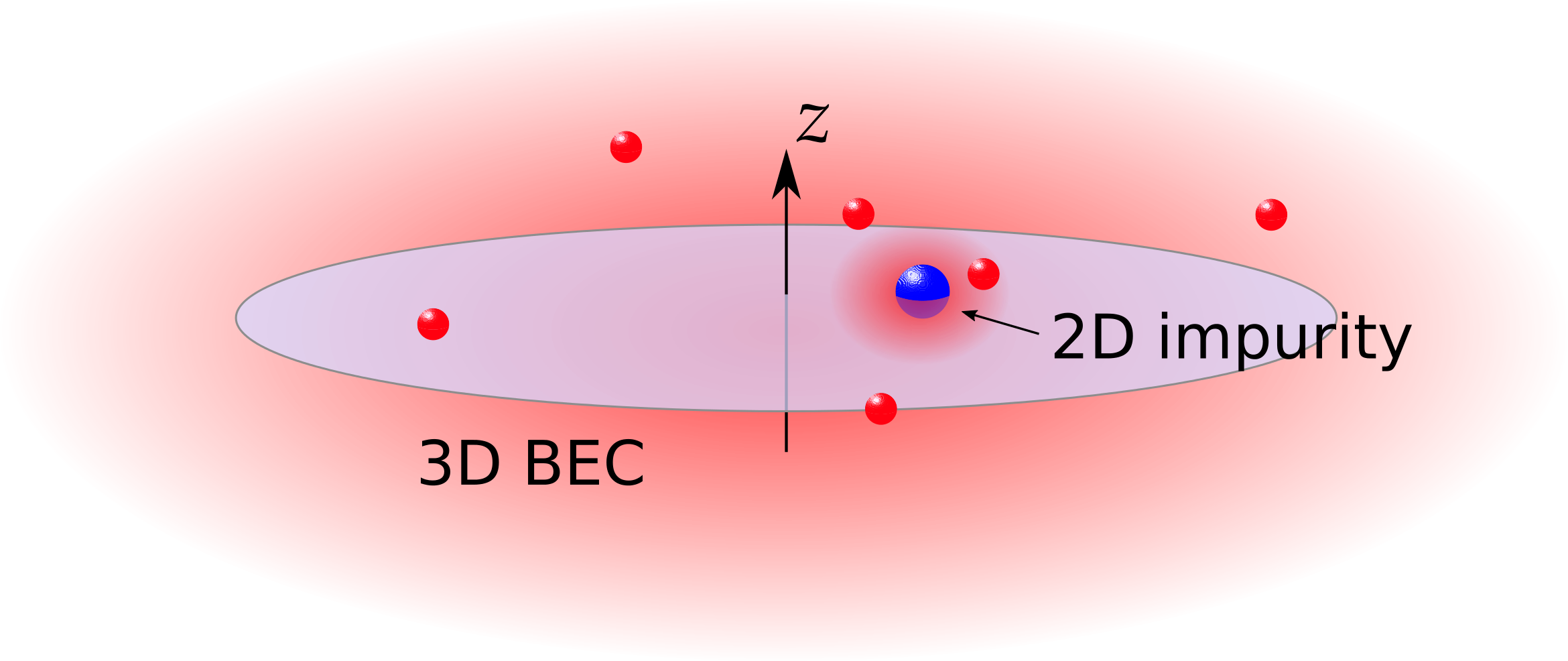
Figure 1: Sketch of the system: 2D impurity particle (blue) immersed in a 3D Bose-Einstein condensate (red).

II Model

We consider a single impurity atom of mass $m$ confined in the 2D $xy$-plane by a strong harmonic trap $m\omega_{z}^{2}z^{2}/2$ along the $z$-direction. Since only one impurity is considered, our results of course do not depend on the statistics of the impurity. For concreteness, we take the impurity to be a fermion. The impurity atom is immersed in a weakly interacting 3D Bose gas of atoms with mass $m_{B}$ (see Fig. 1). The bosons form a BEC with density $n_{0}$, which is accurately described by Bogoliubov theory since we assume $n_{0}^{1/3}a_{B}\ll 1$, where $a_{B}$ is the boson scattering length. The Hamiltonian of the system is

$$H=\sum_{{\bf p}_{\perp}}\frac{{\bf p}_{\perp}^{2}}{2m}a_{{\bf p}_{\perp}}^{\dagger}a_{{\bf p}_{\perp}}+\sum_{{\bf p}}E_{\bf p}\gamma_{\bf p}^{\dagger}\gamma_{\bf p}+H_{\text{int}}\;,$$ (1)

where $a_{{\bf p}_{\perp}}^{\dagger}$ creates an impurity with 2D momentum ${\bf p}_{\perp}=(p_{x},p_{y})$, and $\gamma_{\bf p}^{\dagger}$ creates Bogoliubov mode in the BEC with 3D momentum ${\bf p}$ and energy $E_{\bf p}=\sqrt{\epsilon_{\bf p}(\epsilon_{\bf p}+2n_{B}g_{B})}$. Here $\epsilon_{\bf p}={\bf p}^{2}/2m_{B}$ and $g_{B}=4\pi a_{B}/m_{B}$. Throughout this paper, we set $\hbar=k_{B}=1$. For clarity we will use the $\perp$ sign to denote vectors in the plane in order to distinguish them from the 3D vectors. The interaction between the bosons and the impurity is

$$H_{\text{int}}=\frac{1}{\mathcal{V}}\sum_{{\bf p}{\bf p}^{\prime}_{\perp}{\bf q}}e^{-(q_{z}l_{z}/2)^{2}}V({\bf q})b^{\dagger}_{{\bf p}+{\bf q}}a^{\dagger}_{{\bf p}^{\prime}_{\perp}-{\bf q}_{\perp}}a_{{\bf p}^{\prime}_{\perp}}b_{{\bf p}}\;,$$ (2)

where ${\bf q}=({\bf q}_{\perp},q_{z})$, $l_{z}=1/\sqrt{m\omega_{z}}$ is the harmonic oscillator length for the vertical trap and $V({\bf q})$ is the boson-fermion interaction potential. The latter will later be eliminated in favor of the effective 2D-3D scattering length $a_{\rm eff}$. The operator $b_{\bf p}^{\dagger}$ creates a boson with momentum ${\bf p}$, and it is related to the Bogoliubov mode creation operators by the usual relation $b_{\bf p}=u_{\bf p}\gamma_{\bf p}-v_{\bf p}\gamma^{\dagger}_{-{\bf p}}$ with $u_{\bf p}^{2}=[(\epsilon_{\bf p}+g_{B}n_{B})/E_{\bf p}+1]/2$ and $v_{\bf p}^{2}=[(\epsilon_{\bf p}+g_{B}n_{B})/E_{\bf p}-1]/2$. We have in Eq. (2) assumed that due to the strong confinement, the impurity resides in the lowest harmonic oscillator state $\phi_{0}(z)=\exp\left\{-z^{2}/2l_{z}^{2}\right\}/\pi^{1/4}\sqrt{l_{z}}$ in the $z$-direction. The exponential factor in Eq. (2) comes from the Fourier transform of $\phi_{0}(z)$. Note that only transverse momentum is conserved during boson-impurity collisions due to the confinement of the impurity in the vertical direction.

III Self-energy

We employ the ladder approximation to calculate the self-energy of the Bose polaron Rath and Schmidt (2013). For the Fermi polaron, this approximation has proven to be surprisingly accurate even for strong interactions Chevy (2006); Prokof’ev and Svistunov (2008); Mora and Chevy (2009); Punk et al. (2009); Combescot et al. (2009); Massignan and Bruun (2011); Massignan et al. (2014). The accuracy of the ladder approximation is less clear for the Bose polaron since there is no Pauli principle, which suppresses more than one fermion from being close to the impurity. The ladder approximation neglects such higher order correlations, which for instance can lead to the formation of a 3-body Efimov state consisting of the impurity atom and two bosons. In Ref. Levinsen et al. (2015), it was shown that these Efimov correlations are important when the scattering length $a_{-}$ for which the first Efimov trimer occurs, is comparable to or smaller than the interparticle distance in the BEC, whereas their effects are small for larger $a_{-}$. It has also been shown that the Efimov effect is suppressed in reduced dimensions as compared to the pure 3D case Nishida and Tan (2011). We therefore assume that higher order correlations are suppressed in the mixed dimensional geometry, and we resort to the ladder approximation in the following.

Figure 2: Diagrams used in the ladder approximation for the impurity. A solid line represents an impurity propagator, a dashed line denotes a boson propagator, and a dotted line denotes a boson emitted or absorbed by the BEC. a) The polaron self-energy given by the sum of the diagrams $\Sigma_{0}$ and $\Sigma_{1}$. b) The $\mathcal{T}$-matrix giving the scattering between the impurity and a boson.

Within the ladder approximation, the polaron self-energy for momentum-frequency $({\bf k}_{\perp},i\omega_{n})$ is given by (see Fig. 2a)

$$\Sigma({\bf k}_{\perp},i\omega_{n})=\Sigma_{0}({\bf k}_{\perp},i\omega_{n})+\Sigma_{1}({\bf k}_{\perp},i\omega_{n})$$ (3)

where

$$\Sigma_{0}({\bf k}_{\perp},i\omega_{n})=n_{B}\mathcal{T}({\bf k}_{\perp},i\omega_{n})$$ (4)

describes the scattering of bosons out of the condensate by the impurity. Here $\omega_{n}=(2n+1)\pi T$ is a fermionic Matsubara frequency where $T$ is the temperature and $n$ is an integer, and $\mathcal{T}$ is the mixed dimension scattering matrix (see below). The self-energy coming from the scattering of bosons not in the condensate is

$$\Sigma_{1}({\bf k}_{\perp},i\omega_{n}) =-T\sum_{\nu}\int\!\frac{d^{3}p}{(2\pi)^{3}}G_{11}({\bf p},i\omega_{\nu})$$

$$\qquad\qquad\quad\times\mathcal{T}({\bf k}_{\perp}+{\bf p}_{\perp},i\omega_{n}+i\omega_{\nu}),$$ (5)

where $\omega_{\nu}=2\nu\pi T$ is a bosonic Matsubara frequency with $\nu$ being an integer. The normal Bogoliubov Green’s function for the bosons is

$$G_{11}({\bf q},i\omega_{\nu})=\frac{u_{\bf q}^{2}}{i\omega_{\nu}-E_{\bf q}}-\frac{v_{\bf q}^{2}}{i\omega_{\nu}+E_{\bf q}}\;.$$ (6)

The 2D-3D scattering matrix between the impurity and a boson can be written as (see Fig. 2b) Nishida (2009)

$$\mathcal{T}({\bf P}_{\perp},i\omega_{m})=\frac{1}{g^{-1}-\Pi({\bf P}_{\perp},i\omega_{m})}\;.$$ (7)

Here $g=2\pi a_{\text{eff}}/\sqrt{m_{B}m_{r}}$, $m_{r}=mm_{B}/(m+m_{B})$ is the reduced mass, $a_{\text{eff}}$ is the effective 2D-3D scattering length and $\Pi({\bf P}_{\perp},i\omega_{n})$ is the pair propagator. The effective scattering length is a function of the 3D boson-impurity scattering length and the trap harmonic oscillator length $l_{z}$ along the $z$-direction. This leads to several confinement induced resonances, which can be exploited to tune the 2D-3D interaction strength Nishida and Tan (2008).

The mixed-dimensional pair propagator is given by

$$\Pi({\bf P}_{\perp},i\omega_{m})= -T\sum_{\nu}\int\!\frac{d^{3}p}{(2\pi)^{3}}G_{11}({\bf p},i\omega_{\nu})$$

$$\qquad\quad\times G^{0}({\bf P}_{\perp}-{\bf p}_{\perp},i\omega_{m}-i\omega_{\nu})\;,$$ (8)

where $G^{0}({\bf q},i\omega_{n})=[i\omega_{n}-\xi_{\bf q}]^{-1}$ is the bare impurity propagator with $\xi_{\bf q}={\bf q}^{2}/2m-\mu$ the bare energy relative to the impurity chemical potential, $\mu$, taken to minus infinity since there is only a single impurity. Performing the Matsubara summation we arrive at

$$\Pi({\bf P}_{\perp},i\omega_{m}) =\int\frac{d^{3}p}{(2\pi)^{3}}\left[\frac{u_{\bf p}^{2}(1+f_{\bf p})}{i\omega_{m}-E_{\bf p}-\xi_{{\bf P}_{\perp}-{\bf p}_{\perp}}}\right.$$

$$+ \left.\frac{v_{\bf p}^{2}f_{\bf p}}{i\omega_{m}+E_{\bf p}-\xi_{{\bf P}_{\perp}-{\bf p}_{\perp}}}+\frac{2m_{B}}{p^{2}+p_{\perp}^{2}/\alpha}\right],$$ (9)

where $f_{\bf p}=[\exp(E_{\bf p}/T)-1]^{-1}$ is the Bose distribution function and $\alpha=m/m_{B}$ is the ratio of the impurity and boson masses. The last term in the brackets in Eq. (9) comes from the regularization of the pair propagator by identifying the molecular pole of the $\mathcal{T}$-matrix at zero center-of-mass momentum in vacuum with $\omega_{M}=-1/2m_{r}a_{\text{eff}}^{2}$ for $a_{\text{eff}}>0$ Nishida (2009).

Equations (3)-(9) have the usual structure of the ladder approximation for a 3D Fermi polaron apart from two differences: First, the scattering medium is a BEC which involves processes describing the scattering of bosons into and out of the condensate; second, the mixed dimension 2D-3D scattering geometry has no intrinsic rotational symmetry, which complicates the evaluation of the resulting integrals significantly compared to the usual 3D case, as we shall discuss below.

IV Quasiparticle properties

The quasiparticle properties of the mixed dimension polaron are encapsulated in the single-particle retarded Green’s function

$$G({\bf k}_{\perp},\omega)=\frac{1}{\omega+i0^{+}-\Sigma({\bf k}_{\perp},\omega)},$$ (10)

where $\Sigma({\bf k}_{\perp},\omega)$ is the retarded polaron self-energy obtained from performing the analytical continuation $i\omega_{n}+\mu\rightarrow\omega+i0^{+}$. To characterize the quasiparticle, we calculate its dispersion, residue, and effective mass. The quasiparticle dispersion $\varepsilon_{{\bf k}_{\perp}}$ for a given momentum ${\bf k}_{\perp}$ is found by solving the self-consistent equation

$$\varepsilon_{{\bf k}_{\perp}}=\frac{{\bf k}_{\perp}^{2}}{2m}+\mathfrak{Re}\Sigma({\bf k}_{\perp},\varepsilon_{{\bf k}_{\perp}})\;,$$ (11)

where we assume that the damping (determined by the imaginary part of $\Sigma$) of the polaron is small. The quasiparticle residue is

$$Z_{{\bf k}_{\perp}}=\frac{1}{1-\partial_{\omega}\mathfrak{Re}\Sigma({\bf k}_{\perp},\omega)|_{\omega=\varepsilon_{{\bf k}_{\perp}}}}\;,$$ (12)

and the effective mass is

$$m^{*}_{{\bf k}_{\perp}}=\frac{Z_{{\bf k}_{\perp}}^{-1}}{m^{-1}+k_{\perp}^{-1}\partial_{k_{\perp}}\mathfrak{Re}\Sigma({\bf k}_{\perp},\omega)|_{\omega=\varepsilon_{{\bf k}_{\perp}}}}\;.$$ (13)

It should be noted that $\Sigma$ only depends on the length of ${\bf k}_{\perp}$, denoted $k_{\perp}$ above. We shall also calculate the spectral function of the polaron defined as

$$A({\bf k}_{\perp},\omega)=-2\mathfrak{Im}G({\bf k}_{\perp},\omega)\;.$$ (14)

V Numerical calculation

The mixed dimensional geometry turns out to significantly complicate the numerical calculation of the polaron self-energy. The reason is that the scattering of the impurity on a boson does not conserve momentum along the $z$-direction and therefore has no rotational symmetry, which can be used to reduce the number of convoluted integrals in the self-energy. This means that in order to make progress, we have to use simplifications for the calculation of $\Sigma_{1}({\bf k}_{\perp},\omega)$ given by Eq. (5), which involves six convoluted integrals. For $\Sigma_{1}({\bf k}_{\perp},\omega)$ we shall approximate the mixed dimension pair propagator by that for a non-interacting Bose gas. Since we focus on the case of zero temperature, the pair propagator is then given by the vacuum expression

$$\Pi_{\rm vac}({\bf P}_{\perp},i\omega_{m})=-i\,\frac{\sqrt{m_{B}}m_{r}}{\sqrt{2}\pi}\sqrt{i\omega_{m}+\mu-\frac{{\bf P}_{\perp}^{2}}{2M}}\;,$$ (15)

where $M=m+m_{B}$ and the complex square root is taken in the upper half plane. Physically, this approximation corresponds to assuming that the boson-impurity scattering is unaffected by the BEC medium, which is a good approximation for momenta $p\gtrsim 1/\xi_{B}$, where $\xi_{B}=1/\sqrt{8\pi n_{0}a_{B}}$ is the coherence length of the BEC. With this approximation, the numerical evaluation of $\Sigma_{1}({\bf k}_{\perp},\omega)$ becomes feasible. In the following, we shall suppress the momentum label ${\bf k}_{\perp}$ for the polaron, as we only consider the case of a zero momentum polaron ${\bf k}_{\perp}=\bf{0}$. We refer the reader to the appendix for details of the numerical procedure.

VI Results

In this section, we present numerical results for the quasi-particle properties of the Bose polaron. In Fig. 3, we plot the polaron energy $\varepsilon/\varepsilon_{n}$ for zero momentum as a function of the inverse coupling strength $1/k_{n}a_{\text{eff}}$ at zero temperature. We have defined the momentum and energy scales as $k_{n}=(6\pi^{2}n_{B})^{1/3}$ and $\varepsilon_{n}=k_{n}^{2}/2m_{B}$ respectively. The energy is calculated for various gas parameters $n_{0}^{1/3}a_{B}$ of the BEC, and for the mass ratios $\alpha=m/m_{B}=1$ and $\alpha=1,40/87$ relevant for the experiments in Ref. Jørgensen et al. (2016) and Hu et al. (2016).

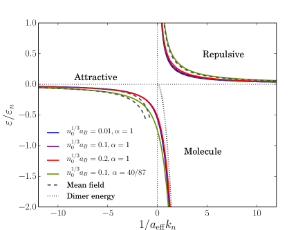
Figure 3: The quasi-particle energy for zero momentum as a function of the inverse Fermi-Bose interaction strength.

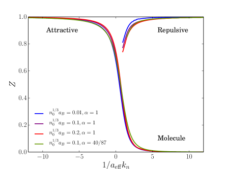
Figure 4: The quasiparticle residue for zero momentum as a function of the inverse Fermi-Bose interaction strength.

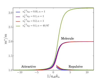
Figure 5: The effective mass for zero momentum as a function of the inverse Fermi-Bose interaction strength.

The corresponding quasiparticle residue and effective mass are plotted in Figs. 4-5. As for the 3D case, we see that there are two polaronic branches: One at negative energy $\varepsilon<0$, which is called attractive polaron, and one at positive energy $\varepsilon>0$, which is called the repulsive polaron.

For weak attractive interactions $1/k_{n}a_{\text{eff}}\lesssim-4$, the energy of the attractive polaron is close to the mean-field result $gn_{B}$, where $n_{B}$ is the total density of the bosons, the residue is $Z\simeq 1$, and the effective mass is $m^{*}\simeq m$. As the attraction is increased, the polaron energy decreases, but it is significantly higher than the mean-field prediction. Contrary to the mean-field prediction, the polaron energy is finite at unitarity $1/k_{n}a_{\text{eff}}=0$, where we find the following quasiparticle properties: $\varepsilon/\varepsilon_{n}\simeq-0.54$, $Z\simeq 0.7$, $m^{*}/m\simeq 1.17$ for $\alpha=1$ and $\varepsilon/\varepsilon_{n}\simeq-0.75$, $Z\simeq 0.7$, $m^{*}/m\simeq 1.26$ for $\alpha=40/87$. These results are universal in the sense that they depend only weakly on the BEC gas parameter in the range $0.01\leq n_{0}^{1/3}a_{B}\leq 0.2$ within the theory, as can be seen from Figs. 3-5. This should be contrasted with the case of a 3D Bose polaron, where a stronger dependence was found using a the same ladder approximation Rath and Schmidt (2013). Although the predicted universality of the polaron energy at unitarity could be an artefact of the ladder approximation, we speculate that the dependence on the gas parameter is suppressed in the mixed dimensional geometry, since the impurity living in 2D affects the bosons living in 3D less. Thus, higher order correlations neglected by the ladder approximation might be less important in the present mixed dimensional geometry so that the polaron has universal properties at unitarity. This is supported by the fact that 3-body Efimov physics is suppressed in mixed dimensional setups as noted above Nishida and Tan (2011). Our theory does not predict any instability as $a_{B}\rightarrow 0$ in contrast to Monte-Carlo calculations for the 3D Bose polaron, where it was associated to the clustering of many bosons around to the impurity Ardila and Giorgini (2015). Similar effects for the 3D Bose polaron were found in Ref. Grusdt et al. (2017). Eventually, the attractive polaron energy approaches the dimer energy $-1/2m_{r}a_{\text{eff}}^{2}$ on the BEC side ($a_{\text{eff}}>0$) of the resonance, the residue approaches zero, and the effective mass approaches $m^{*}=m+m_{B}$. This reflects the fact the impurity has formed a mixed dimensional dimer state with one boson from the BEC, in analogy with what happens for the 3D polaron.

The repulsive polaron is well defined for weak repulsive interactions $1/k_{n}a_{\text{eff}}\gg 1$ with an energy close to the mean-field result $gn_{B}$, a residue $Z\simeq 1$, and an effective mass $m^{*}\simeq m$. As the repulsion increases, the energy and effective mass increase, whereas the residue decreases. We find that the polaron becomes ill defined for strong repulsion $0<1/k_{n}a_{\text{eff}}\lesssim 0.8$, where the numerics cannot find the residue and effective mass due to a large imaginary part of the self-energy.

To investigate this further, we plot in Fig. 6 the spectral function $A(\omega)$ of the polaron as a function of $1/k_{n}a_{\text{eff}}$ for zero temperature and a BEC gas parameter $n_{0}^{1/3}a_{B}=0.1$.

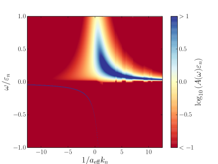
Figure 6: The spectral function of the zero momentum polaron as a function of frequency and inverse Fermi-Bose interaction strength.

As expected, the attractive polaron gives rise to a sharp peak with a width given by the small imaginary part $i\delta/\varepsilon_{n}\leq i10^{-5}$, which is added by hand to the frequency in the numerical calculations. We see that there is also a continuum of spectral weight for $\omega>0$. This continuum corresponds to states consisting of an impurity with transverse momentum ${\bf p}_{\perp}$ and a Bogoliubov mode with momentum ${\bf p}=(-{\bf p}_{\perp},p_{z})$. Since the ladder approximation treats the scattered impurity as a bare particle, the energy of these continuum states are predicted to be $\omega={\bf p}_{\perp}^{2}/2m+E_{\bf p}$ with a threshold at $\omega=0$. This is however not physical since the scattered impurity also forms a polaron, and a more elaborate theory including self-consistent impurity propagators in all diagrams would yield a continuum starting just above the polaron quasiparticle peak on the attractive side $a_{\text{eff}}<0$ of the resonance Rath and Schmidt (2013).

We see from Fig. 6 that the polaron peak on the repulsive side $a_{\text{eff}}>0$ is strongly damped as the interaction is increased towards the unitarity limit. This is because it sits right in the middle of the continuum described above. It is due to this strong damping that the repulsive polaron residue and effective mass cannot be calculated for $1/k_{n}a_{\text{eff}}\lesssim 0.8$ as can be seen from Figs. 4-5. This result for the damping is however not quantitatively reliable since the continuum is not treated in a self-consistent manner as noted above. Also, we have not included 3-body decay of the repulsive polaron into the dimer state Fedichev et al. (1996); Petrov (2003); Massignan and Bruun (2011). Nevertheless, we expect the non-zero damping of the repulsive polaron predicted by the ladder approximation to be qualitatively correct, since it does contain the 2-body decay into a Bogoliubov mode and a scattered impurity in an approximate way, which likely is dominant in analogy with the 3D case Massignan and Bruun (2011).

VII Conclusions

In conclusion, we analysed a mixed dimensional Bose polaron, where the impurity particle moves in a 2D plane immersed in a 3D BEC. Using a diagrammatic ladder approximation that includes the mixed dimensional 2D-3D vacuum scattering between the impurity and the bosons exactly, the mixed dimensional polaron was shown to exhibit the same qualitative features as the pure 3D Bose-polaron. In particular, there is a well defined polaron state for attractive impurity-boson interaction that smoothly develops into a mixed dimensional dimer for strong attraction, and there is a well defined polaron state for weak repulsive interaction, which becomes strongly damped as the repulsion increases. As opposed to the 3D case, our calculations predict that the properties of the polaron are almost independent of the gas parameter of the BEC as long as it is small so that Bogoliubov theory applies. It follows that the polaron has universal properties in the unitarity limit of the impurity-boson interaction. We speculate that higher order correlations, which could change this result, are suppressed in the mixed dimensional geometry. The fact that we predict well-defined quasiparticles in mixed dimensional systems indicates that these systems should be well described by Fermi liquid theory, which will be interesting to investigate in the future.

Appendix A Appendix

In this appendix we derive the expressions we implemented numerically to obtain the results discussed in the paper. We will also comment on the approximations used in order to obtain an efficient numerical code.

First we derive expressions for $\Sigma_{0}({\bf k}_{\perp},\omega)$ and $\Sigma_{1}({\bf k}_{\perp},\omega)$ that sum to be the polaron self-energy $\Sigma({\bf k}_{\perp},\omega)$, the key ingredient in all further computations. From the self-energy we may directly evaluate the spectral function $A({\bf k}_{\perp},\omega)$ from Eq. (14) and obtain the quasiparticle energy $\varepsilon_{{\bf k}_{\perp}}$ as the solution to Eq. (11). The quasiparticle residue $Z_{{\bf k}_{\perp}}$ and the effective mass $m^{*}_{{\bf k}_{\perp}}$ given by Eqs. (12)–(13) require the derivatives of the self-energy.

A.1 $\Sigma_{0}$ and its derivatives

Computation of $\Sigma_{0}({\bf k}_{\perp},\omega)$ as given in Eq. (4) requires the pair propagator given in Eq. (9) with $i\omega_{m}+\mu\rightarrow\omega+i0^{+}$. In this section we consider the following:

$$\Sigma_{0}(\bm{0},\omega)=\frac{n_{B}}{g^{-1}-\Pi(\bm{0},\omega)}$$ (16)

$$\partial_{\omega}\Sigma_{0}(\bm{0},\omega)=\frac{1}{n_{B}}(\Sigma_{0}(\bm{0},\omega))^{2}\partial_{\omega}\Pi(\bm{0},\omega)$$ (17)

$$k_{\perp}^{-1}\partial_{k_{\perp}}\Sigma_{0}({\bf k}_{\perp},\omega)|_{k_{\perp}=0}=\frac{1}{n_{B}}(\Sigma_{0}(\bm{0},\omega))^{2}k_{\perp}^{-1}\partial_{k_{\perp}}\Pi({\bf k}_{\perp},\omega)|_{k_{\perp}=0}.$$ (18)

We start by simplifying the pair propagator by taking the zero-temperature limit, i.e., by setting the Bose distribution function $f_{{\bf p}}=0$. In spherical coordinates the pair propagator becomes:

$$\Pi({\bf k}_{\perp},\omega)=\frac{2m_{B}}{(2\pi)^{3}}\int_{0}^{\infty}dp\,p^{2}\int_{0}^{\pi}d\theta\,\sin\theta\int_{0}^{2\pi}d\phi$$

$$\times\left[\left(\frac{p^{2}+\tilde{g}_{B}}{2\tilde{E}_{p}}+\frac{1}{2}\right)\frac{1}{2m_{B}\omega-\tilde{E}_{p}-\alpha^{-1}(p^{2}\sin^{2}\theta+k_{\perp}^{2}-2pk_{\perp}\sin\theta\cos\phi)+i0^{+}}+\frac{1}{p^{2}(1+\alpha^{-1}\sin^{2}\theta)}\right]$$ (19)

with $\tilde{E}_{p}\equiv\sqrt{p^{2}(p^{2}+2\tilde{g}_{B})}$ and $\tilde{g}_{B}\equiv 2m_{B}g_{B}n_{B}$. The integral over $\phi$ is trivial when $k_{\perp}=0$, but it can be performed also in the case $k_{\perp}\neq 0$. In the latter case, we let $z_{0}=(2m_{B}\omega-\tilde{E}_{p}-\alpha^{-1}(p^{2}\sin^{2}\theta+k^{2}_{\perp})+i0^{+})/(2\alpha^{-1}pk_{\perp}\sin\theta)$ located in the upper half complex plane. The $\phi$ integral takes the form $\int_{0}^{2\pi}d\phi\,(z_{0}+\cos\phi)^{-1}=2\pi/(\sqrt{z_{0}-1}\sqrt{z_{0}+1})$, where the complex square roots should be taken in the upper half plane. The integral over $\theta$ can be simplified by defining $x=-\cos\theta$ and substituting $\int_{0}^{\pi}d\theta\,\sin\theta\rightarrow 2\int_{0}^{1}dx$, yielding for the pair propagator:

$$\Pi({\bf k}_{\perp},\omega) =\frac{2m_{B}}{2\pi^{2}}\int_{0}^{\infty}dp\int_{0}^{1}dx\left[\left(\frac{p^{2}+\tilde{g}_{B}}{2\tilde{E}_{p}}+\frac{1}{2}\right)\frac{p^{2}}{\sqrt{z_{+}}\sqrt{z_{-}}}+\frac{1}{1+\alpha^{-1}(1-x^{2})}\right]$$

$$=\frac{2m_{B}}{2\pi^{2}}\int_{0}^{\infty}dp\left[\left(\frac{p^{2}+\tilde{g}_{B}}{2\tilde{E}_{p}}+\frac{1}{2}\right)\int_{0}^{1}dx\frac{p^{2}}{\sqrt{z_{+}}\sqrt{z_{-}}}+\frac{\text{arcsinh}(\alpha^{-1/2})}{\sqrt{\alpha^{-1}(\alpha^{-1}+1)}}\right]$$ (20)

with $z_{\pm}=2m_{B}\omega-\tilde{E}_{p}-\alpha^{-1}(p\sqrt{1-x^{2}}\pm k_{\perp})^{2}+i0^{+}$. In the case $k_{\perp}=0$ the expression reduces to

$$\Pi(\bm{0},\omega) =\frac{2m_{B}}{2\pi^{2}}\int_{0}^{\infty}dp\left[\left(\frac{p^{2}+\tilde{g}_{B}}{2\tilde{E}_{p}}+\frac{1}{2}\right)\int_{0}^{1}dx\frac{p^{2}}{2m_{B}\omega-\tilde{E}_{p}-\alpha^{-1}p^{2}(1-x^{2})+i0^{+}}+\frac{\text{arcsinh}(\alpha^{-1/2})}{\sqrt{\alpha^{-1}(\alpha^{-1}+1)}}\right]$$

$$=\frac{2m_{B}}{2\pi^{2}}\int_{0}^{\infty}dp\left[\left(\frac{p^{2}+\tilde{g}_{B}}{2\tilde{E}_{p}}+\frac{1}{2}\right)\mathcal{P}\int_{0}^{1}dx\frac{p^{2}}{2m_{B}\omega-\tilde{E}_{p}-\alpha^{-1}p^{2}(1-x^{2})}+\frac{\text{arcsinh}(\alpha^{-1/2})}{\sqrt{\alpha^{-1}(\alpha^{-1}+1)}}\right]$$

$$-i\pi\frac{2m_{B}}{2\pi^{2}}\int_{0}^{\infty}dp\,p^{2}\left(\frac{p^{2}+\tilde{g}_{B}}{2\tilde{E}_{p}}+\frac{1}{2}\right)\int_{0}^{1}dx\,\delta(2m_{B}\omega-\tilde{E}_{p}-\alpha^{-1}p^{2}(1-x^{2}))\;.$$ (21)

The second equality separates the real and imaginary part of the integral. Here $\mathcal{P}$ denotes the Cauchy principal value integral and $\delta(x)$ is the Dirac delta function. In practice we use the first line in Eq. (21) to calculate the real part of the integral by setting $0^{+}$ to a positive number which is sufficiently small. We let $z_{1}=(2m_{B}\omega-\tilde{E}_{p}-\alpha^{-1}p^{2}+i0^{+})\alpha/p^{2}$ and take the $x$ integral as $\int_{0}^{1}dx\,(z_{1}+x^{2})^{-1}=\text{arccot}(\sqrt{z_{1}})/\sqrt{z_{1}}$ with the complex square root taken in the upper half plane. Hence

$$\mathfrak{Re}\Pi(\bm{0},\omega)=\frac{2m_{B}}{2\pi^{2}}\int_{0}^{\infty}dp\left[\left(\frac{p^{2}+\tilde{g}_{B}}{2\tilde{E}_{p}}+\frac{1}{2}\right)\mathfrak{Re}\left(\frac{\alpha\,\text{arccot}(\sqrt{z_{1}})}{\sqrt{z_{1}}}\right)+\frac{\text{arcsinh}(\alpha^{-1/2})}{\sqrt{\alpha^{-1}(\alpha^{-1}+1)}}\right]\;.$$ (22)

For the imaginary part of the pair propagator, we define a new variable $u=1-x^{2}$ and the function $u_{\delta}(p)=(2m_{B}\omega-\tilde{E}_{p})\alpha/p^{2}$ which allows us to express

$$\mathfrak{Im}\Pi(\bm{0},\omega)=-\frac{2m_{B}}{2\pi}\int_{0}^{\infty}dp\,\left(\frac{p^{2}+\tilde{g}_{B}}{2\tilde{E}_{p}}+\frac{1}{2}\right)\int_{0}^{1}du\,\frac{\alpha}{2\sqrt{1-u}}\delta(u_{\delta}(p)-u)\;.$$ (23)

The Dirac delta function is only non-vanishing along the $u$ integration interval for those values of $p$ where $0<u_{\delta}(p)<1$. Notice that this implies that $\mathfrak{Im}\Pi(\bm{0},\omega)=0$ for $\omega\leq 0$. In the case $\omega>0$ we have to determine the values of $p$ in the integration interval that fulfill $0<u_{\delta}(p)<1$. Formally we may define this set as $\mathcal{V}=\{p\in(0;\infty)\,\colon u_{\delta}(p)\in(0;1)\}$. Since the Dirac delta function contributes only when $p\in\mathcal{V}$, we have

$$\mathfrak{Im}\Pi(\bm{0},\omega)=-\frac{2m_{B}}{2\pi}\int_{\mathcal{V}}dp\,\left(\frac{p^{2}+\tilde{g}_{B}}{2\tilde{E}_{p}}+\frac{1}{2}\right)\frac{\alpha}{2\sqrt{1-u_{\delta}(p)}}\;.$$ (24)

We now prove that $\mathcal{V}$ is an interval. First notice that $u_{\delta}(p)\rightarrow\infty$ as $p\rightarrow 0$ and $u_{\delta}(p)\rightarrow-\alpha<0$ as $p\rightarrow\infty$. Since $u_{\delta}$ is continous the inequality $0<u_{\delta}(p)<1$ is indeed fulfilled somewhere along the $p$ integration. Second we notice from explicit computation that the equation $du_{\delta}/dp=0$ has at most one real solution on $(0;\infty)$ which must correspond to a global minimum. Thus $u_{\delta}$ decreases monotonically in the region where $0<u_{\delta}(p)<1$. We conclude that $\mathcal{V}=(p_{\text{min}};p_{\text{max}})$ with the end points uniquely defined by $u_{\delta}(p_{\text{min}})=1$ and $u_{\delta}(p_{\text{max}})=0$. Explicitly we have

$$p_{\text{min}}=\begin{cases}\sqrt{\frac{-\tilde{g}_{B}\alpha^{2}-\omega\alpha-\alpha\sqrt{(\tilde{g}_{B}^{2}+\omega^{2})\alpha^{2}+2\tilde{g}_{B}\omega\alpha}}{\alpha^{2}-1}}&\text{if }\alpha<1\\ \sqrt{\frac{\omega^{2}}{2(\tilde{g}_{B}+\omega)}}&\text{if }\alpha=1\\ \sqrt{\frac{-\tilde{g}_{B}\alpha^{2}-\omega\alpha+\alpha\sqrt{(\tilde{g}_{B}^{2}+\omega^{2})\alpha^{2}+2\tilde{g}_{B}\omega\alpha}}{\alpha^{2}-1}}&\text{if }\alpha>1\end{cases}\qquad\text{and}\qquad p_{\text{max}}=\sqrt{-\tilde{g}_{B}+\sqrt{\tilde{g}_{B}^{2}+\omega^{2}}}.$$ (25)

The imaginary part of the pair propagator takes the final form:

$$\mathfrak{Im}\Pi(\bm{0},\omega)=\begin{cases}0&\text{if }\omega\leq 0\\ -\frac{2m_{B}}{2\pi}\int_{p_{\text{min}}}^{p_{\text{max}}}dp\,\left(\frac{p^{2}+\tilde{g}_{B}}{2\tilde{E}_{p}}+\frac{1}{2}\right)\frac{\alpha}{2\sqrt{1-(2m_{B}\omega-\tilde{E}_{p})\alpha/p^{2}}}&\text{if }\omega>0.\end{cases}$$ (26)

We now turn to the derivatives of the pair propagator appearing in Eqs. (17)–(18). From Eq. (20) we find

$$\partial_{\omega}\Pi({\bf k}_{\perp},\omega)=\frac{(2m_{B})^{2}}{2\pi^{2}}\int_{0}^{\infty}dp\left(\frac{p^{2}+\tilde{g}_{B}}{2\tilde{E}_{p}}+\frac{1}{2}\right)\int_{0}^{1}dx\left[\frac{-p^{2}}{2(z_{+})^{3/2}\sqrt{z_{-}}}+\frac{-p^{2}}{2(z_{-})^{3/2}\sqrt{z_{+}}}\right]\;,$$ (27)

which simplifies in the case $k_{\perp}=0$ using $z_{-}=z_{+}$ and $\int_{0}^{1}dx\,(z_{1}+x^{2})^{-2}=(\sqrt{z_{1}}/(z_{1}+1)+\text{arccot}(\sqrt{z_{1}})/(2z_{1}^{3/2})$, where the complex square root should be taken in the upper half plane. We find

$$\partial_{\omega}\Pi({\bf k}_{\perp},\omega)=-\frac{(2m_{B})^{2}}{2\pi^{2}}\int_{0}^{\infty}dp\left(\frac{p^{2}+\tilde{g}_{B}}{2\tilde{E}_{p}}+\frac{1}{2}\right)\frac{\alpha^{2}}{2z_{1}^{3/2}p^{2}}\left[\frac{\sqrt{z_{1}}}{z_{1}+1}+\text{arccot}(\sqrt{z_{1}})\right]\;.$$ (28)

Similarly we find

$$k_{\perp}^{-1}\partial_{k_{\perp}}\Pi({\bf k}_{\perp},\omega)= \frac{2m_{B}}{2\pi^{2}}\int_{0}^{\infty}dp\left(\frac{p^{2}+\tilde{g}_{B}}{2\tilde{E}_{p}}+\frac{1}{2}\right)$$

$$\int_{0}^{1}dx\frac{-p^{2}2\alpha^{-1}k_{\perp}(\alpha^{-1}(k_{\perp}-p\sqrt{1-x^{2}})(k_{\perp}+p\sqrt{1-x^{2}})-2m_{B}\omega+\tilde{E}_{p}-i0^{+})}{z_{+}^{3/2}z_{-}^{3/2}}\,.$$ (29)

Notice that we may safely put $k_{\perp}=0$ in the above expression and evaluate the $x$ integral:

$$k_{\perp}^{-1}\partial_{k_{\perp}}\Pi({\bf k}_{\perp},\omega)|_{k_{\perp}=0}=\frac{2m_{B}}{\pi^{2}}\int_{0}^{\infty}dp\left(\frac{p^{2}+\tilde{g}_{B}}{2\tilde{E}_{p}}+\frac{1}{2}\right)\frac{p^{2}}{\alpha}\int_{0}^{1}dx\,\frac{2m_{B}\omega-\tilde{E}_{p}+i0^{+}+\alpha^{-1}p^{2}(1-x^{2})}{(2m_{B}\omega-\tilde{E}_{p}+i0^{+}-\alpha^{-1}p^{2}(1-x^{2}))^{3}}$$ (30)

$$=\frac{2m_{B}}{4\pi^{2}\alpha}\int_{0}^{\infty}dp\left(\frac{p^{2}+\tilde{g}_{B}}{2\tilde{E}_{p}}+\frac{1}{2}\right)p^{2}\left[\frac{3}{(2m_{B}\omega-\tilde{E}_{p}+i0^{+}-\alpha^{-1}p^{2})^{2}}+\frac{\sqrt{\alpha}(2m_{B}\omega-\tilde{E}_{p}+i0^{+}+2\alpha^{-1}p^{2})\text{arccot}(z_{1})}{p(2m_{B}\omega-\tilde{E}_{p}+i0^{+}-\alpha^{-1}p^{2})^{5/2}}\right]\;.$$ (31)

This concludes the derivations of the numerical integrals we implemented in order to compute Eqs. (16)–(18).

A.2 $\Sigma_{1}$ and its derivatives

In this section we shall compute $\Sigma_{1}(\bm{0},\omega)$ and the derivatives $\partial_{\omega}\Sigma_{1}(\bm{0},\omega)$ and $k_{\perp}^{-1}\partial_{k_{\perp}}\Sigma_{1}({\bf k}_{\perp},\omega)|_{k_{\perp}=0}$. From Eq. (5), with $i\omega_{n}+\mu\rightarrow\omega+i0^{+}$, we have

$$\Sigma_{1}({\bf k}_{\perp},\omega) =-T\sum_{\nu}\int\frac{d^{3}p}{(2\pi)^{3}}\left.\left(\frac{u_{\bf p}^{2}}{i\omega_{\nu}-E_{\bf p}}-\frac{v_{\bf p}^{2}}{i\omega_{\nu}+E_{\bf p}}\right)\frac{1}{g^{-1}-\Pi({\bf p}_{\perp}+{\bf k}_{\perp},i\omega_{n}+i\omega_{\nu})}\right|_{i\omega_{n}+\mu\rightarrow\omega+i0^{+}}$$ (32)

$$=\int\frac{d^{3}p}{(2\pi)^{3}}\frac{v_{\bf p}^{2}}{g^{-1}-\Pi({\bf p}_{\perp}+{\bf k}_{\perp},\omega-E_{\bf p})}\;,$$ (33)

where the last line is found from performing the sum over Matsubara frequencies and letting the temperature $T\rightarrow 0$. Here we exploit that the chemical potential $\mu$ is minus infinity such that any poles and branch cuts of the $\mathcal{T}$-matrix are pushed to infinity.

We have to simplify the expression above in order to get a numerical feasible implementation. Therefore we approximate the pair propagator by that for a non-interaction Bose gas at zero temperature $\Pi_{\rm vac}$. This amounts to setting $g_{B}=0$ and $f_{\bf p}=0$ in Eq. (9). We now show that it reduces to the expression in Eq. (15). Notice that these approximations are only applied to the pair propagator, as setting the temperature to zero in the entire expression for $\Sigma_{1}$ would make it vanish, and this we are definitely not interested in. The pair propagator takes the form

$$\Pi_{\rm vac}({\bf p}_{\perp},\omega-E_{\bf p})=\int\frac{d^{3}\tilde{p}}{(2\pi)^{3}}\left[\frac{1}{\omega-E_{\bf p}-\tilde{p}^{2}/2m_{B}-({\bf k}_{\perp}+{\bf p}_{\perp}+\tilde{\bf p}_{\perp})^{2}/2m+i0^{+}}+\frac{2m_{B}}{\tilde{p}^{2}+\tilde{p}_{\perp}^{2}/\alpha}\right]\;.$$ (34)

We shift $\tilde{\bf p}$ in the first term in the integrand by adding the constant vector ${\bf p}\,m_{B}/M$. Then we scale $\tilde{\bf p}_{\perp}$ in the entire integrand by the factor $\sqrt{m/M}$ such that the integral, with $z^{\prime}=2m_{B}(\omega-E_{\bf p}-({\bf p}_{\perp}+{\bf k}_{\perp})^{2}/2M+i0^{+})$, becomes

$$\Pi_{\rm vac}({\bf p}_{\perp}+{\bf k}_{\perp},\omega-E_{\bf p}) =\frac{2m_{B}}{1+\alpha^{-1}}\int\frac{d^{3}\tilde{p}}{(2\pi)^{3}}\left[\frac{1}{z^{\prime}-\tilde{p}^{2}}+\frac{1}{\tilde{p}^{2}}\right]$$ (35)

$$=\frac{2m_{B}}{2\pi^{2}(1+\alpha^{-1})}\int_{0}^{\infty}d\tilde{p}\,\frac{z^{\prime}}{z^{\prime}-\tilde{p}^{2}}$$ (36)

$$=-\frac{2m_{B}z^{\prime}}{4\pi^{2}(1+\alpha^{-1})}\int_{-\infty}^{\infty}d\tilde{p}\,\frac{1}{(\tilde{p}+\sqrt{z^{\prime}})(\tilde{p}-\sqrt{z^{\prime}})}\;.$$ (37)

Noting that the pole at $\sqrt{z^{\prime}}$ is located in the upper half complex plane, we perform the contour integral around the pole yielding $\int_{-\infty}^{\infty}d\tilde{p}\,[(\tilde{p}+\sqrt{z^{\prime}})(\tilde{p}-\sqrt{z^{\prime}})]^{-1}=i\pi/\sqrt{z^{\prime}}$. The pair propagator simplifies to

$$\Pi_{\rm vac}({\bf p}_{\perp}+{\bf k}_{\perp},\omega-E_{\bf p})=\begin{cases}-i\frac{\sqrt{m_{B}}m_{r}}{\sqrt{2}\pi}\sqrt{|\omega-E_{\bf p}-({\bf p}_{\perp}+{\bf k}_{\perp})^{2}/2M|}&\qquad\text{if }\;\omega-E_{\bf p}-({\bf p}_{\perp}+{\bf k}_{\perp})^{2}/2M\geq 0\\[10.00002pt] \frac{\sqrt{m_{B}}m_{r}}{\sqrt{2}\pi}\sqrt{|\omega-E_{\bf p}-({\bf p}_{\perp}+{\bf k}_{\perp})^{2}/2M|}&\qquad\text{if }\;\omega-E_{\bf p}-({\bf p}_{\perp}+{\bf k}_{\perp})^{2}/2M<0\end{cases}$$ (38)

which is equivalent to the expression in Eq. (15).

Returning to $\Sigma_{1}$ from Eq. (33) we go to spherical coordinates $(p,\theta,\phi)$ and substitute $x=-\cos\theta$:

$$\Sigma_{1}({\bf k}_{\perp},\omega)=\frac{1}{2\pi^{3}}\int_{0}^{\infty}dp\,\int_{0}^{1}dx\,\int_{0}^{\pi}d\phi\frac{p^{2}\,v_{\bf p}^{2}}{g^{-1}-e^{i\psi_{-}}\frac{\sqrt{m_{B}}m_{r}}{\sqrt{2}\pi}\sqrt{|\omega-E_{\bf p}-(k_{\perp}^{2}+p^{2}(1-x^{2})+2k_{\perp}p\sqrt{1-x^{2}}\cos\phi)/2M|}}\;,$$ (39)

where $e^{i\psi_{\pm}}\in\{1,-i\}$ are integration variable dependent phase factors given according to Eq. (38). In the case $k_{\perp}=0$ the $\phi$ integration is trivial, and we get

$$\Sigma_{1}(\bm{0},\omega)=\frac{1}{2\pi^{2}}\int_{0}^{\infty}dp\,\int_{0}^{1}dx\,\frac{p^{2}\,v_{\bf p}^{2}}{g^{-1}-e^{i\psi_{-}}\frac{\sqrt{m_{B}}m_{r}}{\sqrt{2}\pi}\sqrt{|\omega-E_{\bf p}-p^{2}(1-x^{2})/2M|}}\;.$$ (40)

The derivate of $\Sigma_{1}(\bm{0},\omega)$ with respect to $\omega$ is straight-forward to compute:

$$\partial_{\omega}\Sigma_{1}(\bm{0},\omega)=-\frac{\sqrt{m_{B}}m_{r}}{4\sqrt{2}\pi^{3}}\int_{0}^{\infty}dp\,\int_{0}^{1}dx\,\frac{p^{2}\,v_{\bf p}^{2}\,e^{i\psi_{-}}(\omega-E_{\bf p}-p^{2}(1-x^{2})/2M)}{|\omega-E_{\bf p}-p^{2}(1-x^{2})/2M|^{3/2}\left(g^{-1}-e^{i\psi_{-}}\frac{\sqrt{m_{B}}m_{r}}{\sqrt{2}\pi}\sqrt{|\omega-E_{\bf p}-p^{2}(1-x^{2})/2M|}\right)^{2}}\;.$$ (41)

Finally we compute the limit of $k_{\perp}^{-1}\partial_{k_{\perp}}\Sigma_{1}({\bf k}_{\perp},\omega)$ when $k_{\perp}\rightarrow 0$ from Eq. (39). We notice that the integrand of $k_{\perp}^{-1}\partial_{k_{\perp}}\Sigma_{1}({\bf k}_{\perp},\omega)$ consists of two term when $k_{\perp}$ is small. One of the terms is proportional to $k_{\perp}^{-1}\cos\phi$ and the integral over $\phi$ vanishes. The other term is constant with respect to $\phi$ and $k_{\perp}$, and the $\phi$ integral just yields a factor of $\pi$. All taken together, we find that $k_{\perp}^{-1}\partial_{k_{\perp}}\Sigma_{1}({\bf k}_{\perp},\omega)|_{k_{\perp}=0}=-M^{-1}\partial_{\omega}\Sigma_{1}(\bm{0},\omega)$, and so we do not have to implement this formula separately.

References

- Baym and Pethick (1991) G. Baym and C. Pethick, Landau Fermi-Liquid Theory: Concepts and Applications (Wiley-VCH, 1991).
- Landau and Pekar (1948) L. D. Landau and S. I. Pekar, Zh. Eksp. Teor. Fiz. 18, 419 (1948).
- Mahan (2000) G. Mahan, Many-Particle Physics (Kluwer Academic/Plenum Publishers, 2000).
- Weinberg (1995) S. Weinberg, The Quantum Theory of Fields, The Quantum Theory of Fields 3 Volume Hardback Set No. vb. 1 (Cambridge University Press, 1995).
- Chin et al. (2010) C. Chin, R. Grimm, P. Julienne, and E. Tiesinga, Rev. Mod. Phys. 82, 1225 (2010).
- Schirotzek et al. (2009) A. Schirotzek, C.-H. Wu, A. Sommer, and M. W. Zwierlein, Phys. Rev. Lett. 102, 230402 (2009).
- Kohstall et al. (2012) C. Kohstall, M. Zaccanti, M. Jag, A. Trenkwalder, P. Massignan, G. M. Bruun, F. Schreck, and R. Grimm, Nature 485, 615 (2012).
- Koschorreck et al. (2012) M. Koschorreck, D. Pertot, E. Vogt, B. Fröhlich, M. Feld, and M. Köhl, Nature (London) 485, 619 (2012).
- Chevy (2006) F. Chevy, Phys. Rev. A 74, 063628 (2006).
- Prokof’ev and Svistunov (2008) N. Prokof’ev and B. Svistunov, Phys. Rev. B 77, 020408 (2008).
- Mora and Chevy (2009) C. Mora and F. Chevy, Phys. Rev. A 80, 033607 (2009).
- Punk et al. (2009) M. Punk, P. T. Dumitrescu, and W. Zwerger, Phys. Rev. A 80, 053605 (2009).
- Combescot et al. (2009) R. Combescot, S. Giraud, and X. Leyronas, EPL (Europhysics Letters) 88, 60007 (2009).
- Cui and Zhai (2010) X. Cui and H. Zhai, Phys. Rev. A 81, 041602 (2010).
- Massignan and Bruun (2011) P. Massignan and G. M. Bruun, European Physical Journal D 65, 83 (2011), arXiv:1102.0121 .
- Massignan et al. (2014) P. Massignan, M. Zaccanti, and G. M. Bruun, Reports on Progress in Physics 77, 034401 (2014).
- Yi and Cui (2015) W. Yi and X. Cui, Phys. Rev. A 92, 013620 (2015).
- Catani et al. (2012) J. Catani, G. Lamporesi, D. Naik, M. Gring, M. Inguscio, F. Minardi, A. Kantian, and T. Giamarchi, Phys. Rev. A 85, 023623 (2012).
- Jørgensen et al. (2016) N. B. Jørgensen, L. Wacker, K. T. Skalmstang, M. M. Parish, J. Levinsen, R. S. Christensen, G. M. Bruun, and J. J. Arlt, Phys. Rev. Lett. 117, 055302 (2016).
- Hu et al. (2016) M.-G. Hu, M. J. Van de Graaff, D. Kedar, J. P. Corson, E. A. Cornell, and D. S. Jin, Phys. Rev. Lett. 117, 055301 (2016).
- Cucchietti and Timmermans (2006) F. M. Cucchietti and E. Timmermans, Phys. Rev. Lett. 96, 210401 (2006).
- Huang and Wan (2009) B.-B. Huang and S.-L. Wan, Chinese Physics Letters 26, 080302 (2009).
- Tempere et al. (2009) J. Tempere, W. Casteels, M. K. Oberthaler, S. Knoop, E. Timmermans, and J. T. Devreese, Phys. Rev. B 80, 184504 (2009).
- Grusdt et al. (2015) F. Grusdt, Y. E. Shchadilova, A. N. Rubtsov, and E. Demler, Scientific Reports 5, 12124 EP (2015).
- Christensen et al. (2015) R. S. Christensen, J. Levinsen, and G. M. Bruun, Phys. Rev. Lett. 115, 160401 (2015).
- Rath and Schmidt (2013) S. P. Rath and R. Schmidt, Phys. Rev. A 88, 053632 (2013).
- Levinsen et al. (2015) J. Levinsen, M. M. Parish, and G. M. Bruun, Phys. Rev. Lett. 115, 125302 (2015).
- Shchadilova et al. (2016) Y. E. Shchadilova, R. Schmidt, F. Grusdt, and E. Demler, Phys. Rev. Lett. 117, 113002 (2016).
- Ardila and Giorgini (2015) L. A. P. Ardila and S. Giorgini, Phys. Rev. A 92, 033612 (2015).
- Ardila and Giorgini (2016) L. A. P. Ardila and S. Giorgini, Phys. Rev. A 94, 063640 (2016).
- Sun et al. (2017) M. Sun, H. Zhai, and X. Cui, arXiv:1702.06303 (2017).
- Lamporesi et al. (2010) G. Lamporesi, J. Catani, G. Barontini, Y. Nishida, M. Inguscio, and F. Minardi, Phys. Rev. Lett. 104, 153202 (2010).
- McKay et al. (2013) D. C. McKay, C. Meldgin, D. Chen, and B. DeMarco, Phys. Rev. Lett. 111, 063002 (2013).
- Jotzu et al. (2015) G. Jotzu, M. Messer, F. Görg, D. Greif, R. Desbuquois, and T. Esslinger, Phys. Rev. Lett. 115, 073002 (2015).
- LeBlanc and Thywissen (2007) L. J. LeBlanc and J. H. Thywissen, Phys. Rev. A 75, 053612 (2007).
- Catani et al. (2009) J. Catani, G. Barontini, G. Lamporesi, F. Rabatti, G. Thalhammer, F. Minardi, S. Stringari, and M. Inguscio, Phys. Rev. Lett. 103, 140401 (2009).
- Haller et al. (2010) E. Haller, M. J. Mark, R. Hart, J. G. Danzl, L. Reichsöllner, V. Melezhik, P. Schmelcher, and H.-C. Nägerl, Phys. Rev. Lett. 104, 153203 (2010).
- Nishida and Tan (2008) Y. Nishida and S. Tan, Phys. Rev. Lett. 101, 170401 (2008).
- Suchet et al. (2017) D. Suchet, Z. Wu, F. Chevy, and G. M. Bruun, Phys. Rev. A 95, 043643 (2017).
- Cheng et al. (2017) Y. Cheng, R. Zhang, P. Zhang, and H. Zhai, arXiv:1705.06878 (2017).
- Iskin and Subaş ı (2010) M. Iskin and A. L. Subaş ı, Phys. Rev. A 82, 063628 (2010).
- Okamoto et al. (2017) J. Okamoto, L. Mathey, and W.-M. Huang, ArXiv e-prints (2017), arXiv:1701.03273 [cond-mat.quant-gas] .
- Nishida (2009) Y. Nishida, Annals of Physics 324, 897 (2009).
- Kim et al. (2013) D.-H. Kim, J. S. J. Lehikoinen, and P. Törmä, Phys. Rev. Lett. 110, 055301 (2013).
- Wu and Bruun (2016) Z. Wu and G. M. Bruun, Phys. Rev. Lett. 117, 245302 (2016).
- Melkær Midtgaard et al. (2017) J. Melkær Midtgaard, Z. Wu, and G. M. Bruun, ArXiv e-prints (2017), arXiv:1705.10169 [cond-mat.quant-gas] .
- Nishida and Tan (2011) Y. Nishida and S. Tan, Few-Body Systems 51, 191 (2011).
- Grusdt et al. (2017) F. Grusdt, R. Schmidt, Y. E. Shchadilova, and E. A. Demler, ArXiv e-prints (2017), arXiv:1704.02605 [cond-mat.quant-gas] .
- Fedichev et al. (1996) P. O. Fedichev, M. W. Reynolds, and G. V. Shlyapnikov, Phys. Rev. Lett. 77, 2921 (1996).
- Petrov (2003) D. S. Petrov, Phys. Rev. A 67, 010703 (2003).