Robust and Efficient Transfer Learning with Hidden Parameter Markov Decision Processes

Abstract

We introduce a new formulation of the Hidden Parameter Markov Decision Process (HiP-MDP), a framework for modeling families of related tasks using low-dimensional latent embeddings. Our new framework correctly models the joint uncertainty in the latent parameters and the state space. We also replace the original Gaussian Process-based model with a Bayesian Neural Network, enabling more scalable inference. Thus, we expand the scope of the HiP-MDP to applications with higher dimensions and more complex dynamics.

1 Introduction

The world is filled with families of tasks with similar, but not identical, dynamics. For example, consider the task of training a robot to swing a bat with unknown length $l$ and mass $m$. The task is a member of a family of bat-swinging tasks. If a robot has already learned to swing several bats with various lengths and masses $\{(l_{i},m_{i})\}_{i=1}^{N}$, then the robot should learn to swing a new bat with length $l^{\prime}$ and mass $m^{\prime}$ more efficiently than learning from scratch. That is, it is grossly inefficient to develop a control policy from scratch each time a unique task is encountered.

The Hidden Parameter Markov Decision Process (HiP-MDP) [14] was developed to address this type of transfer learning, where optimal policies are adapted to subtle variations within tasks in an efficient and robust manner. Specifically, the HiP-MDP paradigm introduced a low-dimensional latent task parameterization $w_{b}$ that, combined with a state and action, completely describes the system’s dynamics $T(s^{\prime}|s,a,w_{b})$. However, the original formulation did not account for nonlinear interactions between the latent parameterization and the state space when approximating these dynamics, which required all states to be visited during training. In addition, the original framework scaled poorly because it used Gaussian Processes (GPs) as basis functions for approximating the task’s dynamics.

We present a new HiP-MDP formulation that models interactions between the latent parameters $w_{b}$ and the state $s$ when transitioning to state $s^{\prime}$ after taking action $a$. We do so by including the latent parameters $w_{b}$, the state $s$, and the action $a$ as input to a Bayesian Neural Network (BNN). The BNN both learns the common transition dynamics for a family of tasks and models how the unique variations of a particular instance impact the instance’s overall dynamics. Embedding the latent parameters in this way allows for more accurate uncertainty estimation and more robust transfer when learning a control policy for a new and possibly unique task instance. Our formulation also inherits several desirable properties of BNNs: it can model multimodal and heteroskedastic transition functions, inference scales to data large in both dimension and number of samples, and all output dimensions are jointly modeled, which reduces computation and increases predictive accuracy [11]. Herein, a BNN can capture complex dynamical systems with highly non-linear interactions between state dimensions. Furthermore, model uncertainty is easily quantified through the BNN’s output variance. Thus, we can scale to larger domains than previously possible.

We use the improved HiP-MDP formulation to develop control policies for acting in a simple two-dimensional navigation domain, playing acrobot [42], and designing treatment plans for simulated patients with HIV [15]. The HiP-MDP rapidly determines the dynamics of new instances, enabling us to quickly find near-optimal instance-specific control policies.

2 Background

Model-based reinforcement learning

We consider reinforcement learning (RL) problems in which an agent acts in a continuous state space $S\subseteq\mathbb{R}^{D}$ and a discrete action space $A$. We assume that the environment has some true transition dynamics $T(s^{\prime}|s,a)$, unknown to the agent, and we are given a reward function $R(s,a):S\times A\rightarrow\mathbb{R}$ that provides the utility of taking action $a$ from state $s$. In the model-based reinforcement learning setting, our goal is to learn an approximate transition function $\hat{T}(s^{\prime}|s,a)$ based on observed transitions $(s,a,s^{\prime})$ and then use $\hat{T}(s^{\prime}|s,a)$ to learn a policy $a=\pi(s)$ that maximizes long-term expected rewards $E[\sum_{t}\gamma^{t}r_{t}]$, where $\gamma\in(0,1]$ governs the relative importance of immediate and future rewards.

HiP-MDPs

A HiP-MDP [14] describes a family of Markov Decision Processes (MDPs) and is defined by the tuple $\left\{S,A,W,T,R,\gamma,P_{W}\right\}$, where $S$ is the set of states $s$, $A$ is the set of actions $a$, and $R$ is the reward function. The transition dynamics $T\left(s^{\prime}|s,a,w_{b}\right)$ for each task instance $b$ depend on the value of the hidden parameters $w_{b}\in W$; for each instance, the parameters $w_{b}$ are drawn from prior $P_{W}$. The HiP-MDP framework assumes that a finite-dimensional array of hidden parameters $w_{b}$ can fully specify variations among the true task dynamics. It also assumes the system dynamics are invariant during a task and the agent is signaled when one task ends and another begins.

Bayesian Neural Networks

A Bayesian Neural Network (BNN) is a neural network, $f(\cdot,\cdot;\mathcal{W})$, in which the parameters $\mathcal{W}$ are random variables with some prior $P(\mathcal{W})$ [27]. We place independent Gaussian priors on each parameter $P(\mathcal{W})=\prod_{w\in\mathcal{W}}\mathcal{N}(w;\mu,\sigma^{2})$. Exact Bayesian inference for the posterior over parameters $P(\mathcal{W}|\{(s^{\prime},s,a)\})$ is intractable, but several recent techniques have been developed to scale inference in BNNs [4, 17, 22, 33]. As probabilistic models, BNNs reduce the tendency of neural networks to overfit in the presence of low amounts of data—just as GPs do. In general, training a BNN is more computationally efficient than a GP [22], while still providing coherent uncertainty measurements. Specifically, predictive distributions can be calculated by taking averages over samples of $\mathcal{W}$ from an approximated posterior distribution over the parameters. As such, BNNs are being adopted in the estimation of stochastic dynamical systems [11, 18]..

3 A HiP-MDP with Joint-Uncertainty

The original HiP-MDP transition function models variation across task instances as:

$$s^{\prime}_{d} \approx\sum_{k=1}^{K}w_{bk}\hat{T}^{(\textit{GP})}_{kad}(s)+\epsilon$$

$$w_{bk} \sim\mathcal{N}(\mu_{w_{k}},\sigma^{2}_{w})$$

$$\epsilon \sim\mathcal{N}(0,\sigma^{2}_{ad}),$$ (1)

where $s_{d}$ is the $d^{th}$ dimension of $s$. Each basis transition function $\hat{T}_{kad}$ (indexed by the $k^{th}$ latent parameter, the action $a$, and the dimension $d$) is a GP using only $s$ as input, linearly combined with instance-specific weights $w_{bk}$. Inference involves learning the parameters for the GP basis functions and the weights for each instance. GPs can robustly approximate stochastic state transitions in continuous dynamical systems in model-based reinforcement learning [9, 35, 36]. GPs have also been widely used in transfer learning outside of RL (e.g. [5]).

While this formulation is expressive, it has limitations. The primary limitation is that the uncertainty in the latent parameters $w_{kb}$ is modeled independently of the agent’s state uncertainty. Hence, the model does not account for interactions between the latent parameterization $w_{b}$ and the state $s$. As a result, Doshi-Velez and Konidaris [14] required that each task instance $b$ performed the same set of state-action combinations $(s,a)$ during training. While such training may sometimes be possible—e.g. robots that can be driven to identical positions—it is onerous at best and impossible for other systems such as human patients. The secondary limitation is that each output dimension $s_{d}$ is modeled separately as a collection of GP basis functions $\{\hat{T}_{kad}\}_{k=1}^{K}$. The basis functions for output dimension $s_{d}$ are independent of the basis functions for output dimension $s_{d^{\prime}}$, for $d\neq d^{\prime}$. Hence, the model does not account for correlation between output dimensions. Modeling such correlations typically requires knowledge of how dimensions interact in the approximated dynamical system [2, 19]. We choose not to constrain the HiP-MDP with such a priori knowledge since the aim is to provide basis functions that can ascertain these relationships through observed transitions.

To overcome these limitations, we include the instance-specific weights $w_{b}$ as input to the transition function and model all dimensions of the output jointly:

$$s^{\prime} \approx\hat{T}^{(\textit{BNN})}(s,a,w_{b})+\epsilon$$

$$w_{b} \sim\mathcal{N}\left(\mu_{w},\Sigma_{b}\right)$$

$$\epsilon \sim\mathcal{N}\left(0,\sigma^{2}_{n}\right).$$ (2)

This critical modeling change eliminates all of the above limitations: we can learn directly from data as observed—which is abundant in many industrial and health domains—and no longer require highly constrained training procedure. We can also capture the correlations in the outputs of these domains, which occur in many natural processes.

Finally, the computational demands of using GPs as the transition function limited the application of the original HiP-MDP formulation to relatively small domains. In the following, we use a BNN rather than a GP to model this transition function. The computational requirements needed to learn a GP-based transition function makes a direct comparison to our new BNN-based formulation infeasible within our experiments (Section 5). We demonstrate, in Appendix A, that the BNN-based transition model far exceeds the GP-based transition model in both computational and predictive performance. In addition, BNNs naturally produce multi-dimensional outputs $s^{\prime}$ without requiring prior knowledge of the relationships between dimensions. This allows us to directly model output correlations between the $D$ state dimensions, leading to a more unified and coherent transition model. Inference in a larger input space $s,a,w_{b}$ with a large number of samples is tractable using efficient approaches that let us—given a distribution $P(\mathcal{W})$ and input-output tuples $(s,a,s^{\prime})$—estimate a distribution over the latent embedding $P(w_{b})$. This enables more robust, scalable transfer.

Demonstration

We present a toy domain (Figure 1) where an agent is tasked with navigating to a goal region. The state space is continuous $(s\in(-2,2)^{2})$, and action space is discrete $(a\in\{N,E,S,W\})$. Task instances vary the following the domain aspects: the location of a wall that blocks access to the goal region (either to the left of or below the goal region), the orientation of the cardinal directions (i.e. whether taking action North moves the agent up or down), and the direction of a nonlinear wind effect that increases as the agent moves away from the start region. Ignoring the wall and grid boundaries, the transition dynamics are:

$$\Delta x =(-1)^{\theta_{b}}c\big{(}a_{x}-(1-\theta_{b})\beta\sqrt{(x+1.5)^{2}+(y+1.5)^{2}}\big{)}$$

$$\Delta y =(-1)^{\theta_{b}}c\big{(}a_{y}-\theta_{b}\beta\sqrt{(x+1.5)^{2}+(y+1.5)^{2}}\big{)}$$

$$a_{x} =\begin{cases}1&a\in\{E,W\}\\ 0&\text{otherwise}\end{cases}$$

$$a_{y} =\begin{cases}1&a\in\{N,S\}\\ 0&\text{otherwise,}\end{cases}$$

where $c$ is the step-size (without wind), $\theta_{b}\in\{0,1\}$ indicates which of the two classes the instance belongs to and $\beta\in(0,1)$ controls the influence of the wind and is fixed for all instances. The agent is penalized for trying to cross a wall, and each step incurs a small cost until the agent reaches the goal region, encouraging the agent to discover the goal region with the shortest route possible. An episode terminates once the agent enters the goal region or after 100 time steps.

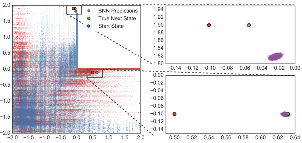
Figure 1: A demonstration of the HiPMDP modeling the joint uncertainty between the latent parameters $w_{b}$ and the state space. On the left, blue and red dots show the exploration during the red ($\theta_{b}=0$) and blue ($\theta_{b}=1$) instances. The latent parameters learned from the red instance are used predict transitions for taking action $E$ from an area of the state space either unexplored (top right) or explored (bottom right) during the red instance. The prediction variance provides an estimate of the joint uncertainty between the latent parameters $w_{b}$ and the state.

A linear function of the state $s$ and latent parameters $w_{b}$ would struggle to model both classes of instances ($\theta_{b}=0$ and $\theta_{b}=1$) in this domain because the state transition resulting from taking an action $a$ is a nonlinear function with interactions between the state and hidden parameter $\theta_{b}$.

By contrast, our new HiP-MDP model allows nonlinear interactions between state and the latent parameters $w_{b}$, as well as jointly models their uncertainty. In Figure 1, this produces measurable differences in transition uncertainty in regions where there are few related observed transitions, even if there are many observations from unrelated instances. Here, the HiP-MDP is trained on two instances from distinct classes (shown in blue ($\theta_{b}=1$) and red ($\theta_{b}=0$) on the left). We display the uncertainty of the transition function, $\hat{T}$, using the latent parameters $w_{\text{red}}$ inferred for a red instance in two regions of the domain: 1) an area explored during red instances and 2) an area not explored under red instances, but explored with blue instances. The transition uncertainty $\hat{T}$ is three times larger in the region where red instances have not been—even if many blue instances have been there—than in regions where red instances have commonly explored, demonstrating that the latent parameters can have different effects on the transition uncertainty in different states.

4 Inference

Algorithm 1 summarizes the inference procedure for learning a policy for a new task instance $b$, facilitated by a pre-trained BNN for that task, and is similar in structure to prior work [9, 18]. The procedure involves several parts. Specifically, at the start of a new instance $b$, we have a global replay buffer $\mathcal{D}$ of all observed transitions $(s,a,r,s^{\prime})$ and a posterior over the weights $\mathcal{W}$ for our BNN transition function $\hat{T}$ learned with data from $\mathcal{D}$. The first objective is to quickly determine the latent embedding, $w_{b}$, of the current instance’s specific dynamical variation as transitions $(s,a,s^{\prime})$ are observed from the current instance. Transitions from instance $b$ are stored in both the global replay buffer $\mathcal{D}$ and an instance-specific replay buffer $\mathcal{D}_{b}$. The second objective is to develop an optimal control policy using the transition model $\hat{T}$ and learned latent parameters $w_{b}$. The transition model $\hat{T}$ and latent embedding $w_{b}$ are separately updated via mini-batch stochastic gradient descent (SGD) using Adam [26]. Using $\hat{T}$ for planning increases our sample efficiency as we reduce interactions with the environment. We describe each of these parts in more detail below.

4.1 Updating embedding $w_{b}$ and BNN parameters $\mathcal{W}$

For each new instance, a new latent weighting $w_{b}$ is sampled from the prior $P_{W}$ (Alg. 1, step 2), in preparation of estimating unobserved dynamics introduced by $\theta_{b}$. Next, we observe transitions $(s,a,r,s^{\prime})$ from the task instance for an initial exploratory episode (Alg. 1, steps 7-10). Given that data, we optimize the latent parameters $w_{b}$ to minimize the $\alpha$-divergence of the posterior predictions of $\hat{T}(s,a,w_{b}|\mathcal{W})$ and the true state transitions $s^{\prime}$ (step 3 in TuneModel) [22]. Here, the minimization occurs by adjusting the latent embedding $w_{b}$ while holding the BNN parameters $\mathcal{W}$ fixed. After an initial update of the $w_{b}$ for a newly encountered instance, the parameters $\mathcal{W}$ of the BNN transition function $\hat{T}$ are optimized (step 4 in TuneModel). As the BNN is trained on multiple instances of a task, we found that the only additional data needed to refine the BNN and latent $w_{b}$ for some new instance can be provided by an initial exploratory episode. Otherwise, additional data from subsequent episodes can be used to further improve the BNN and latent estimates (Alg. 1, steps 11-14).

The mini-batches used for optimizing the latent $w_{b}$ and BNN network parameters $\mathcal{W}$ are sampled from $\mathcal{D}_{b}$ with squared error prioritization [31]. We found that switching between small updates to the latent parameters and small updates to the BNN parameters led to the best transfer performance. If either the BNN network or latent parameters are updated too aggressively (having a large learning rate or excessive number of training epochs), the BNN disregards the latent parameters or state inputs respectively. After completing an instance, the BNN parameters and the latent parameters are updated using samples from global replay buffer $\mathcal{D}$. Specific modeling details such as number of epochs, learning rates, etc. are described in Appendix C.

4.2 Updating policy $\hat{\pi}_{b}$

We construct an $\varepsilon$-greedy policy to select actions based on an approximate action-value function $\hat{Q}(s,a)$. We model the action value function $\hat{Q}(s,a)$ with a Double Deep Q Network (DDQN) [21, 29]. The DDQN involves training two networks (parametrized by $\theta$ and $\theta^{-}$ respectively), a primary Q-network, which informs the policy, and a target Q-network, which is a slowly annealed copy of the primary network (step 9 of SimEp) providing greater stability when updating the policy $\hat{\pi}_{b}$ .

With the updated transition function, $\hat{T}$, we approximate the environment when developing a control policy (SimEp). We simulate batches of entire episodes of length $N_{t}$ using the approximate dynamical model $\hat{T}$, storing each transition in a fictional experience replay buffer $\mathcal{D}^{f}_{b}$ (steps 2-6 in SimEp). The primary network parameters $\theta$ are updated via SGD every $N_{\pi}$ time steps (step 8 in SimEp) to minimize the temporal-difference error between the primary network’s and the target network’s Q-values. The mini-batches used in the update are sampled from the fictional experience replay buffer $\mathcal{D}^{f}_{b}$, using TD-error-based prioritization [38].

Algorithm 1 Learning a control policy w/ the HiP-MDP

1:Input: Global replay buffer $\mathcal{D}$, BNN transition function $\hat{T}$, initial state $s^{0}_{b}$

2:procedure LearnPolicy( $\mathcal{D},\hat{T},s^{0}_{b}$)

3:     Draw new $w_{b}\sim P_{W}$

4:     Randomly init. policy $\hat{\pi}_{b}$ $\theta,\theta^{-}$

5:     Init. instance replay buffer $\mathcal{D}_{b}$

6:     Init. fictional replay buffer $\mathcal{D}^{f}_{b}$

7:     for $i=0$ to $N_{e}$ episodes do

8:         repeat

9:              Take action $a\leftarrow\hat{\pi}_{b}(s)$

10:              Store $\mathcal{D},\mathcal{D}_{b}\leftarrow(s,a,r,s^{\prime},w_{b})$

11:         until episode is complete

12:         if $i=0$ OR $\hat{T}$ is innaccurate then

13:              $\mathcal{D}_{b},\mathcal{W},w_{b}\leftarrow$ TuneModel($\mathcal{D}_{b},\mathcal{W},w_{b}$)

14:              for $j=0$ to $N_{f}-1$ episodes do

15:                  $\mathcal{D}^{f}_{b},\hat{\pi}_{b}\leftarrow$ SimEp($\mathcal{D}^{f}_{b},\hat{T},w_{b},\hat{\pi}_{b},s^{0}_{b}$)                        

16:         $\mathcal{D}^{f}_{b},\hat{\pi}_{b}\leftarrow$ SimEp($\mathcal{D}^{f}_{b},\hat{T},w_{b},\hat{\pi}_{b},s^{0}_{b}$)      

1:function SimEp($\mathcal{D}^{f}_{b},\hat{T},w_{b},\hat{\pi}_{b},s^{0}_{b}$)

2:     for $t=0$ to $N_{t}$ time steps do

3:         Take action $a\leftarrow\hat{\pi}_{b}(s)$

4:         Approx. $\hat{s}^{\prime}\leftarrow\hat{T}(s,a,w_{b})$

5:         Calc. reward $\hat{r}\leftarrow R(s,a,\hat{s}^{\prime})$

6:         Store $\mathcal{D}^{f}_{b}\leftarrow(s,a,\hat{r},\hat{s}^{\prime})$

7:         if $\mod(t,N_{\pi})=0$ then

8:              Update $\hat{\pi}_{b}$ via $\theta$ from $\mathcal{D}^{f}_{b}$

9:              $\theta^{-}\leftarrow\tau\theta+(1-\tau)\theta^{-}$               

10:     return $\mathcal{D}^{f}_{b},\hat{\pi}_{b}$

1:function TuneModel($\mathcal{D}_{b},\mathcal{W},w_{b}$)

2:     for $k=0$ to $N_{u}$ updates do

3:         Update $w_{b}$ from $\mathcal{D}_{b}$

4:         Update $\mathcal{W}$ from $\mathcal{D}_{b}$      

5:     return $\mathcal{D}_{b},\mathcal{W},w_{b}$

5 Experiments and Results

Now, we demonstrate the performance of the HiP-MDP with embedded latent parameters in transferring learning across various instances of the same task. We revisit the 2D demonstration problem from Section 3, as well as describe results on both the acrobot [42] and a more complex healthcare domain: prescribing effective HIV treatments [15] to patients with varying physiologies.

For each of these domains, we compare our formulation of the HiP-MDP with embedded latent parameters (equation 2) with four baselines (one model-free and three model-based) to demonstrate the efficiency of learning a policy for a new instance $b$ using the HiP-MDP. These comparisons are made across the first handful of episodes encountered in a new task instance to highlight the advantage provided by transferring information through the HiP-MDP. The ‘linear’ baseline uses a BNN to learn a set of basis functions that are linearly combined with the parameters $w_{b}$ (used to approximate the approach of Doshi-Velez and Konidaris [14], equation 1), which does not allow interactions between states and weights. The ‘model-based from scratch’ baseline considers each task instance $b$ as unique; requiring the BNN transition function to be trained only on observations made from the current task instance. The ‘average’ model baseline is constructed under the assumption that a single transition function can be used for every instance of the task; $\hat{T}$ is trained from observations of all task instances together. For all model-based approaches, we replicated the HiP-MDP procedure as closely as possible. The BNN was trained on observations from a single episode before being used to generate a large batch of approximate transition data, from which a policy is learned. Finally, the model-free baseline learns a DDQN-policy directly from observations of the current instance.

For more information on the experimental specifications and long-run policy learning see Appendix C and D, respectively.

5.1 Revisiting the 2D demonstration

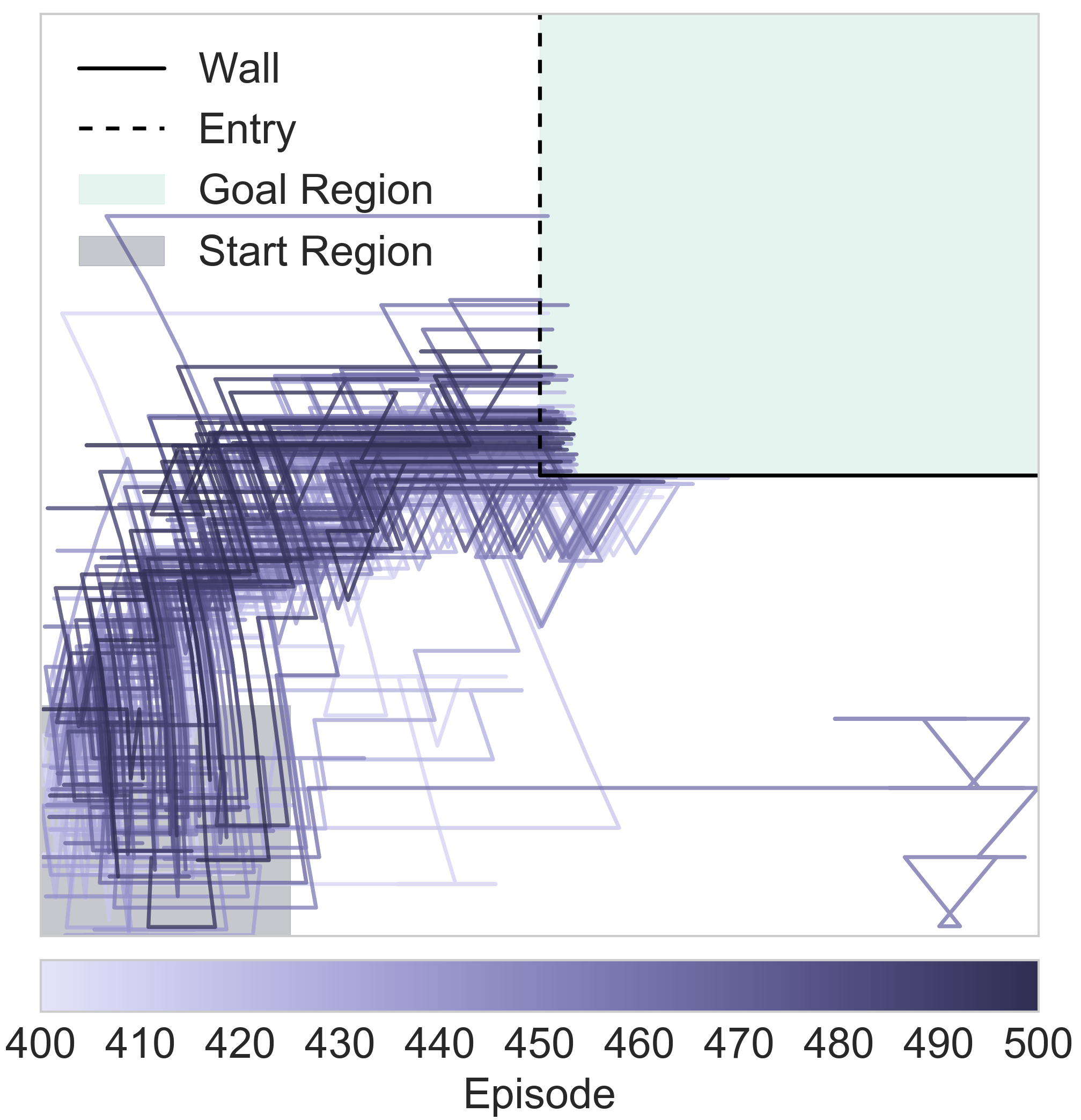
(a)

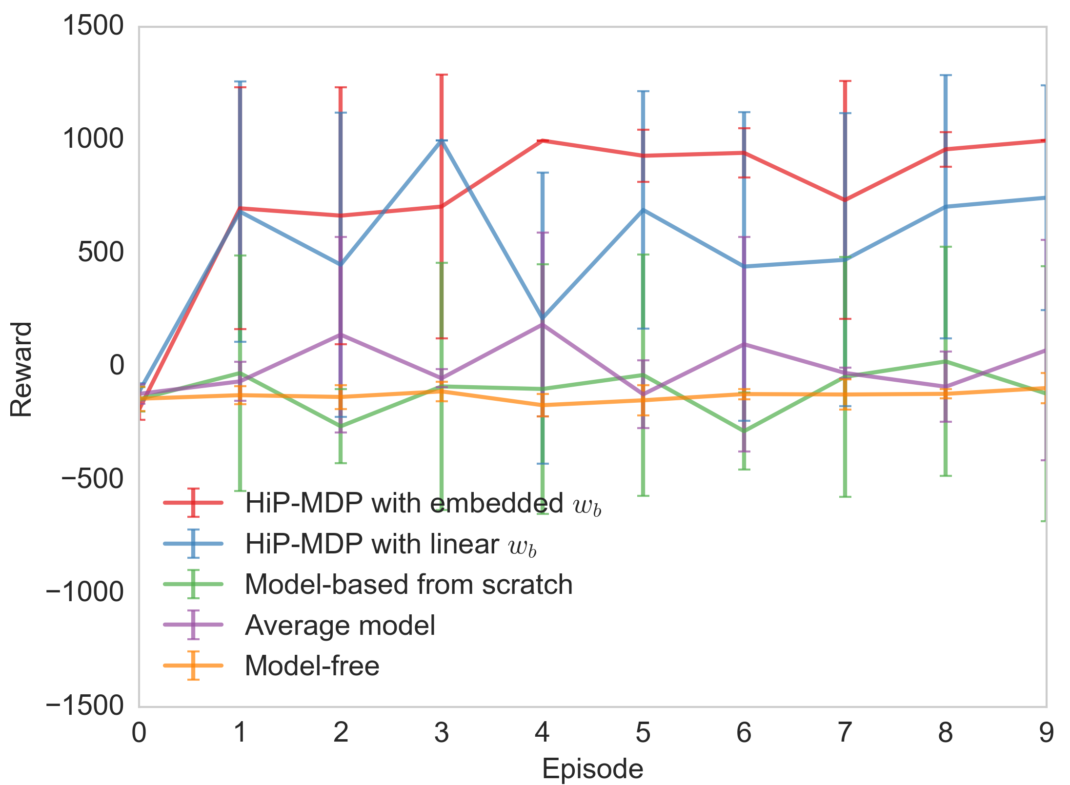
(b)

Figure 2: (a) a demonstration of a model-free control policy, (b) a comparison of learning a policy at the outset of a new task instance $b$ using the HiP-MDP versus four benchmarks. The HiP-MDP with embedded $w_{b}$ outperforms all four benchmarks.

The HiP-MDP and the average model were supplied a transition model $\hat{T}$ trained on two previous instances, one from each class, before being updated according to the procedure outlined in Sec. 4 for a newly encountered instance. After the first exploratory episode, the HiP-MDP has sufficiently determined the latent embedding, evidenced in Figure 2(b) where the developed policy clearly outperforms all four benchmarks. This implies that the transition model $\hat{T}$ adequately provides the accuracy needed to develop an optimal policy, aided by the learned latent parametrization.

The HiP-MDP with linear $w_{b}$ also quickly adapts to the new instance and learns a good policy. However, the HiP-MDP with linear $w_{b}$ is unable to model the nonlinear interaction between the latent parameters and the state. Therefore the model is less accurate and learns a less consistent policy than the HiP-MDP with embedded $w_{b}$. (See Figure 6(a) in Appendix A.2)

With single episode of data, the model trained from scratch on the current instance is not accurate enough to learn a good policy. Training a BNN from scratch requires more observations of the true dynamics than are necessary for the HiP-MDP to learn the latent parameterization and achieve a high level of accuracy. The model-free approach eventually learns an optimal policy, but requires significantly more observations to do so, as represented in Figure 2(a). The model-free approach has no improvement in the first 10 episodes. The poor performance of the average model approach indicates that a single model cannot adequately represent the dynamics of the different task instances. Hence, learning a latent representation of the dynamics specific to each instance is crucial.

5.2 Acrobot

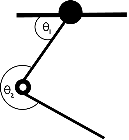
(a)

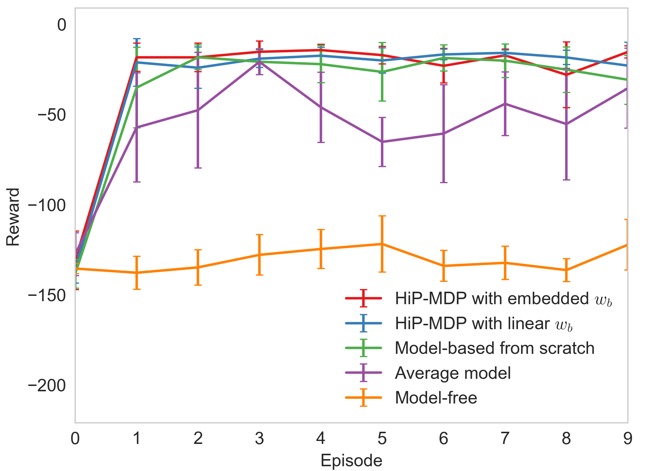
(b)

Figure 3: (a) the acrobot domain, (b) a comparison of learning a policy for a new task instance $b$ using the HiP-MDP versus four benchmarks.

First introduced by Sutton and Barto [42], acrobot is a canonical RL and control problem. The most common objective of this domain is for the agent to swing up a two-link pendulum by applying a positive, neutral, or negative torque on the joint between the two links (see Figure 3(a)). These actions must be performed in sequence such that the tip of the bottom link reaches a predetermined height above the top of the pendulum. The state space consists of the angles $\theta_{1}$, $\theta_{2}$ and angular velocities $\dot{\theta}_{1}$, $\dot{\theta}_{2}$, with hidden parameters corresponding to the masses ($m_{1}$, $m_{2}$) and lengths ($l_{1}$, $l_{2}$), of the two links. See Appendix B.2 for details on how these hidden parameters were varied to create different task instances. A policy learned on one setting of the acrobot will generally perform poorly on other settings of the system, as noted in [3]. Thus, subtle changes in the physical parameters require separate policies to adequately control the varied dynamical behavior introduced. This provides a perfect opportunity to apply the HiP-MDP to transfer between separate acrobot instances when learning a control policy $\hat{\pi}_{b}$ for the current instance.

Figure 3(b) shows that the HiP-MDP learns an optimal policy after a single episode, whereas all other model-based benchmarks required an additional episode of training. As in the toy example, the model-free approach eventually learns an optimal policy, but requires more time.

5.3 HIV treatment

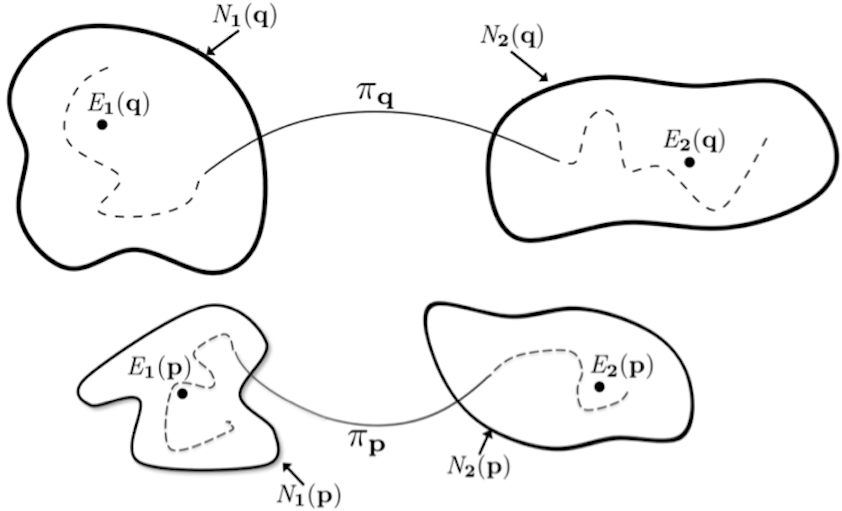
(a)

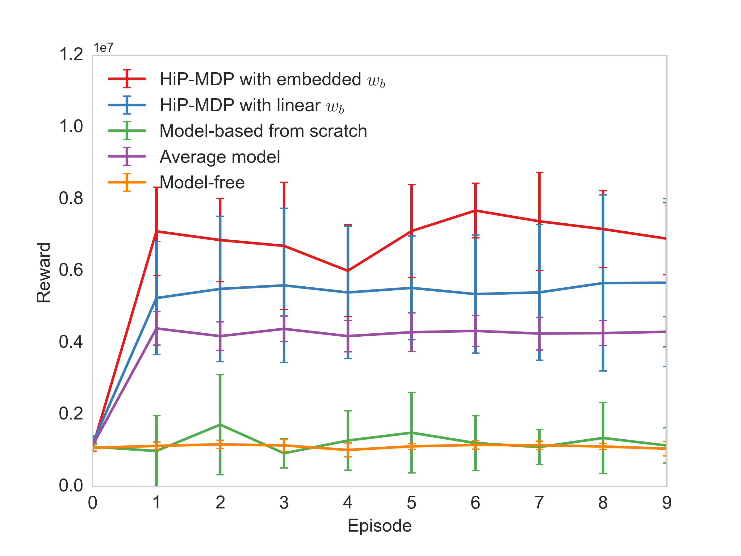
(b)

Figure 4: (a) a visual representation of a patient with HIV transitioning from an unhealthy steady state to a healthy steady state using a proper treatment schedule, (b) a comparison of learning a policy for a new task instance $b$ using the HiP-MDP versus four benchmarks.

Determining effective treatment protocols for patients with HIV was introduced as an RL problem by mathematically representing a patient’s physiological response to separate classes of treatments [1, 15]. In this model, the state of a patient’s health is recorded via 6 separate markers measured with a blood test. Patients are given one of four treatments on a regular schedule. Either they are given treatment from one of two classes of drugs, a mixture of the two treatments, or provided no treatment (effectively a rest period). There are 22 hidden parameters in this system that control a patient’s specific physiology and dictate rates of virulence, cell birth, infection, and death. (See Appendix B.3 for more details.) The objective is to develop a treatment sequence that transitions the patient from an unhealthy steady state to a healthy steady state (Figure 4(a), see adams2004dynamicforamorethoroughexplanation). Small changes made to these parameters can greatly effect the behavior of the system and therefore introduce separate steady state regions that require unique policies to transition between them.

Figure 4(b) shows that the HiP-MDP develops an optimal control policy after a single episode, learning an unmatched optimal policy in the shortest time. The HIV simulator is the most complex of our three domains, and the separation between each benchmark is more pronounced. Modeling a HIV dynamical system from scratch from a single episode of observations proved to be infeasible. The average model, which has been trained off a large batch of observations from related dynamical systems, learns a better policy. The HiP-MDP with linear $w_{b}$ is able to transfer knowledge from previous task instances and quickly learn the latent parameterization for this new instance, leading to an even better policy. However, the dynamical system contains nonlinear interactions between the latent parameters and the state space. Unlike the HiP-MDP with embedded $w_{b}$, the HiP-MDP with linear $w_{b}$ is unable to model those interactions. This demonstrates the superiority of the HiP-MDP with embedded $w_{b}$ for efficiently transferring knowledge between instances in highly complex domains.

6 Related Work

There has been a large body of work on solving single POMDP models efficiently [6, 16, 24, 37, 45]. In contrast, transfer learning approaches leverage training done on one task to perform related tasks. Strategies for transfer learning include: latent variable models, reusing pre-trained model parameters, and learning a mapping between separate tasks (see review in [43]).

Our work falls into the latent variable model category. Using latent representation to relate tasks has been particularly popular in robotics where similar physical movements can be exploited across a variety of tasks and platforms [10, 20]. In Chen et al. [8], these latent representations are encoded as separate MDPs with an accompanying index that an agent learns while adapting to observed variations in the environment. Bai et al. [3] take a closely related approach to our updated formulation of the HiP-MDP by incorporating estimates of unknown or partially observed parameters of a known environmental model and refining those estimates using model-based Bayesian RL. The core difference between this and our work is that we learn the transition model and the observed variations directly from the data while Bai et al. [3] assume it is given and the specific variations of the parameters are learned. Also related are multi-task approaches that train a single model for multiple tasks simultaneously [5, 7]. Finally, there have been many applications of reinforcement learning (e.g. [32, 40, 44]) and transfer learning in the healthcare domain by identifying subgroups with similar response (e.g. [23, 28, 39]).

More broadly, BNNs are powerful probabilistic inference models that allow for the estimation of stochastic dynamical systems [11, 18]. Core to this functionality is their ability to represent both model uncertainty and transition stochasticity [25]. Recent work decomposes these two forms of uncertainty to isolate the separate streams of information to improve learning. Our use of fixed latent variables as input to a BNN helps account for model uncertainty when transferring the pretrained BNN to a new instance of a task. Other approaches use stochastic latent variable inputs to introduce transition stochasticity [12, 30].

We view the HiP-MDP with latent embedding as a methodology that can facilitate personalization and do so robustly as it transfers knowledge of prior observations to the current instance. This approach can be especially useful in extending personalized care to groups of patients with similar diagnoses, but can also be extended to any control system where variations may be present.

7 Discussion and Conclusion

We present a new formulation for transfer learning among related tasks with similar, but not identical dynamics, within the HiP-MDP framework. Our approach leverages a latent embedding—learned and optimized in an online fashion—to approximate the true dynamics of a task. Our adjustment to the HiP-MDP provides robust and efficient learning when faced with varied dynamical systems, unique from those previously learned. It is able, by virtue of transfer learning, to rapidly determine optimal control policies when faced with a unique instance.

The results in this work assume the presence of a large batch of already-collected data. This setting is common in many industrial and health domains, where there may be months, sometimes years, worth of operations data on plant function, product performance, or patient health. Even with large batches, each new instance still requires collapsing the uncertainty around the instance-specific parameters in order to quickly perform well on the task. In Section 5, we used a batch of transition data from multiple instances of a task—without any artificial exploration procedure—to train the BNN and learn the latent parameterizations. Seeded with data from diverse task instances, the BNN and latent parameters accounted for the variation between instances.

While we were primarily interested in settings where batches of observational data exist, one might also be interested in more traditional settings in which the first instance is completely new, the second instance only has information from the first, etc. In our initial explorations, we found that one can indeed learn the BNN in an online manner for simpler domains. However, even with simple domains, the model-selection problem becomes more challenging: an overly expressive BNN can overfit to the first few instances, and have a hard time adapting when it sees data from an instance with very different dynamics. Model-selection approaches to allow the BNN to learn online, starting from scratch, is an interesting future research direction.

Another interesting extension is rapidly identifying the latent $w_{b}$. Exploration to identify $w_{b}$ would supply the dynamical model with the data from the regions of domain with the largest uncertainty. This could lead to a more accurate latent representation of the observed dynamics while also improving the overall accuracy of the transition model. Also, we found training a DQN requires careful exploration strategies. When exploration is constrained too early, the DQN quickly converges to a suboptimal, deterministic policy––often choosing the same action at each step. Training a DQN along the BNN’s trajectories of least certainty could lead to improved coverage of the domain and result in more robust policies. The development of effective policies would be greatly accelerated if exploration were more robust and stable. One could also use the hidden parameters $w_{b}$ to learn a policy directly.

Recognizing structure, through latent embeddings, between task variations enables a form of transfer learning that is both robust and efficient. Our extension of the HiP-MDP demonstrates how embedding a low-dimensional latent representation with the input of an approximate dynamical model facilitates transfer and results in a more accurate model of a complex dynamical system, as interactions between the input state and the latent representation are modeled naturally. We also model correlations in the output dimensions by replacing the GP basis functions of the original HiP-MDP formulation with a BNN. The BNN transition function scales significantly better to larger and more complex problems. Our improvements to the HiP-MDP provide a foundation for robust and efficient transfer learning. Future improvements to this work will contribute to a general transfer learning framework capable of addressing the most nuanced and complex control problems.

Acknowledgements

We thank Mike Hughes, Andrew Miller, Jessica Forde, and Andrew Ross for their helpful conversations. TWK was supported by the MIT Lincoln Laboratory Lincoln Scholars Program. GDK is supported in part by the NIH R01MH109177. The content of this work is solely the responsibility of the authors and does not necessarily represent the official views of the NIH.

Appendix

Appendix A BNN-based transition functions with embedded latent weighting

A.1 Scalability of BNN vs. GP based transition approximation

In this section, we demonstrate the computational motivation to replace the GP basis functions of the original HiP-MDP model [14] with a single, stand-alone BNN as discussed in Sec. 3) using the 2D navigation domain. To fully motivate the replacement, we altered the GP-based model to accept the latent parameters $w_{b}$ and a one-hot encoded action as additional inputs to the transition model. This was done to investigate how the performance of the GP would scale with a higher input dimension; the original formulation of the HiP-MDP [14] uses 2 input dimensions our proposed reformulation of the HiP-MDP uses 11 (2 from the state, 4 from the action and 5 from latent parameterization).

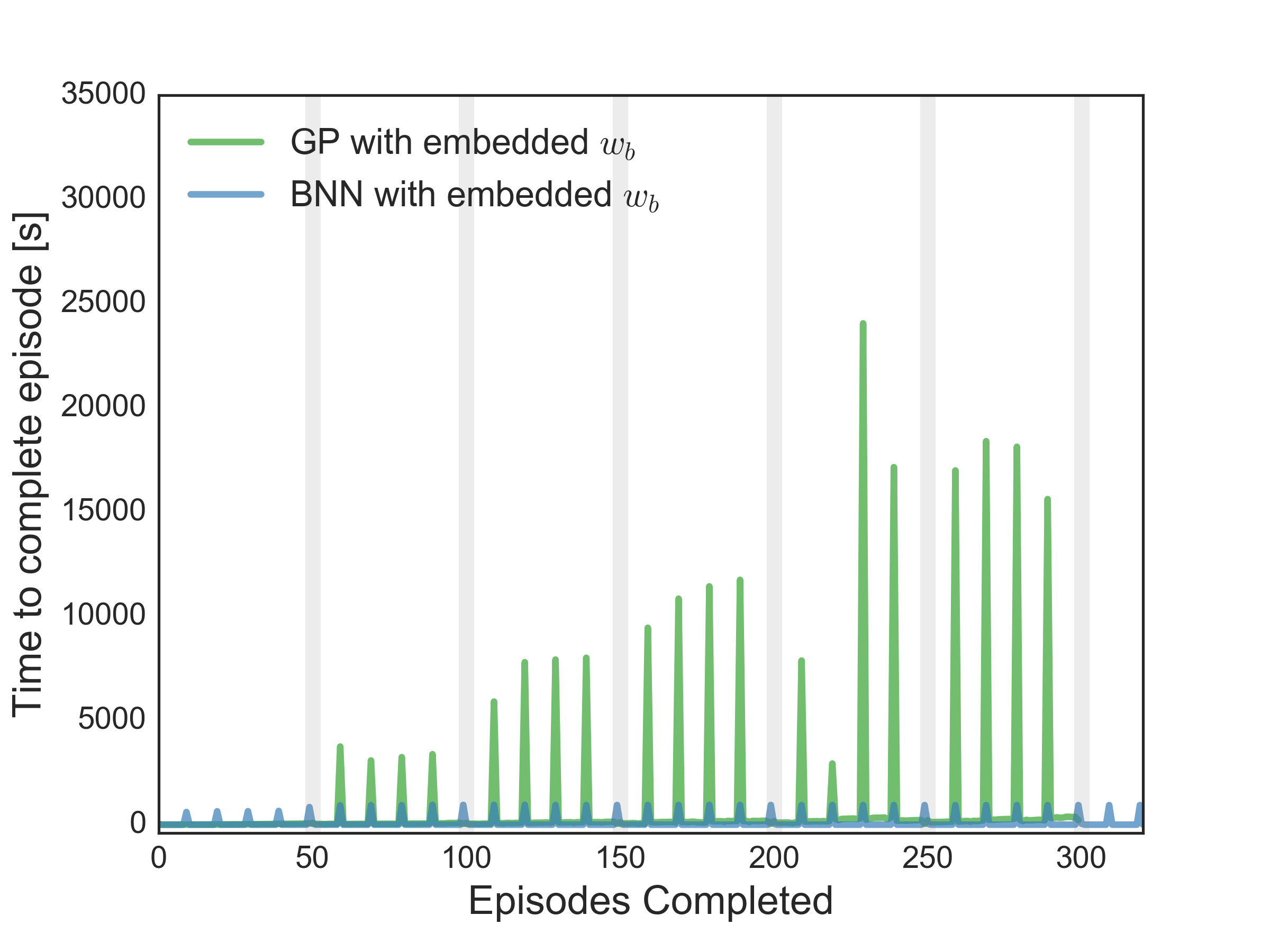
Figure 5: Here we show that the time to run an episode where the approximated transition model $\hat{T}$ and latent parameters $w_{b}$ are updated every 10 episodes. In the 2D navigation domain, the completion time is relatively constant for the BNN, whereas the GP’s completion time drastically increases as more data is collected to construct the transition model.

We directly compare the run-time performance of training both the GP-based and BNN-based HiP-MDP over 6 unique instances of the toy domain, with 50 episodes per instance. Figure 5 shows the running times (in seconds) for each episode of the GP-based HiP-MDP and the BNN-based HiP-MDP, with the transition model $\hat{T}$ and latent parameters $w_{b}$ being updated after every 10 episodes. In stark contrast with the increase in computation for the GP-based HiP-MDP, the BNN-based HiP-MDP has no increase in computation time as more data and further training is encountered. Training the BNN over the course of 300 separate episodes in the 2D toy domain was completed in a little more than 8 hours. In contrast, the GP-based HiP-MDP, trained on the 2D toy domain, took close to 70 hours to complete training on the same number of episodes.

This significant increase in computation time using the GP-based HiP-MDP, on a relatively simple domain, prevented us from performing comparisons to the GP model on our other domains. (We do realize that there is a large literature on making GPs more computationally efficient [13, 34, 41]; we chose to use BNNs because if we were going to make many inference approximations, it seemed reasonable to turn to a model that can easily capture heteroskedastic, multi-modal noise and correlated outputs.)

A.2 Prediction performance: benefit of embedding the latent parameters

In the previous section, we justified replacing the GP basis functions in the HiP-MDP in favor of a BNN. In this section, we investigate the prediction performance of various BNN models to determine whether the latent embedding provides the desired effect of more robust and efficient transfer. The BNN models we will characterize here are those presented in Sec. 5 used as baseline comparisons to the HiP-MDP with embedded latent parameters. These models are:

• HiP-MDP with embedded $w_{b}$

• HiP-MDP with linear $w_{b}$

• BNN learned from scratch, without any latent characterization of the dynamics

• Average model: BNN trained on all data without any latent characterization of the dynamics.

For each of these benchmarks except the BNN trained from scratch, a batch of transition data from previously observed instances was used to pre-train the BNN (and learn the latent parameters for the HiP-MDPs). Each method was then used to learn the dynamics of a new, previously unobserved instance. After the first episode in the newly encountered instance, the BNN is updated. In the two models that use a latent estimation of the environment, the latent parameters are also updated. As can be seen in Fig 6, the models using a latent parameterization improve greatly after those first network and latent parameter updates. The other two (the model from scratch and average model) also improve, but only marginally. The average model is unable to account for the different dynamics of the new instance, and the model trained from scratch does not have enough observed transition data from the new instance to construct an accurate representation of the transition dynamics.

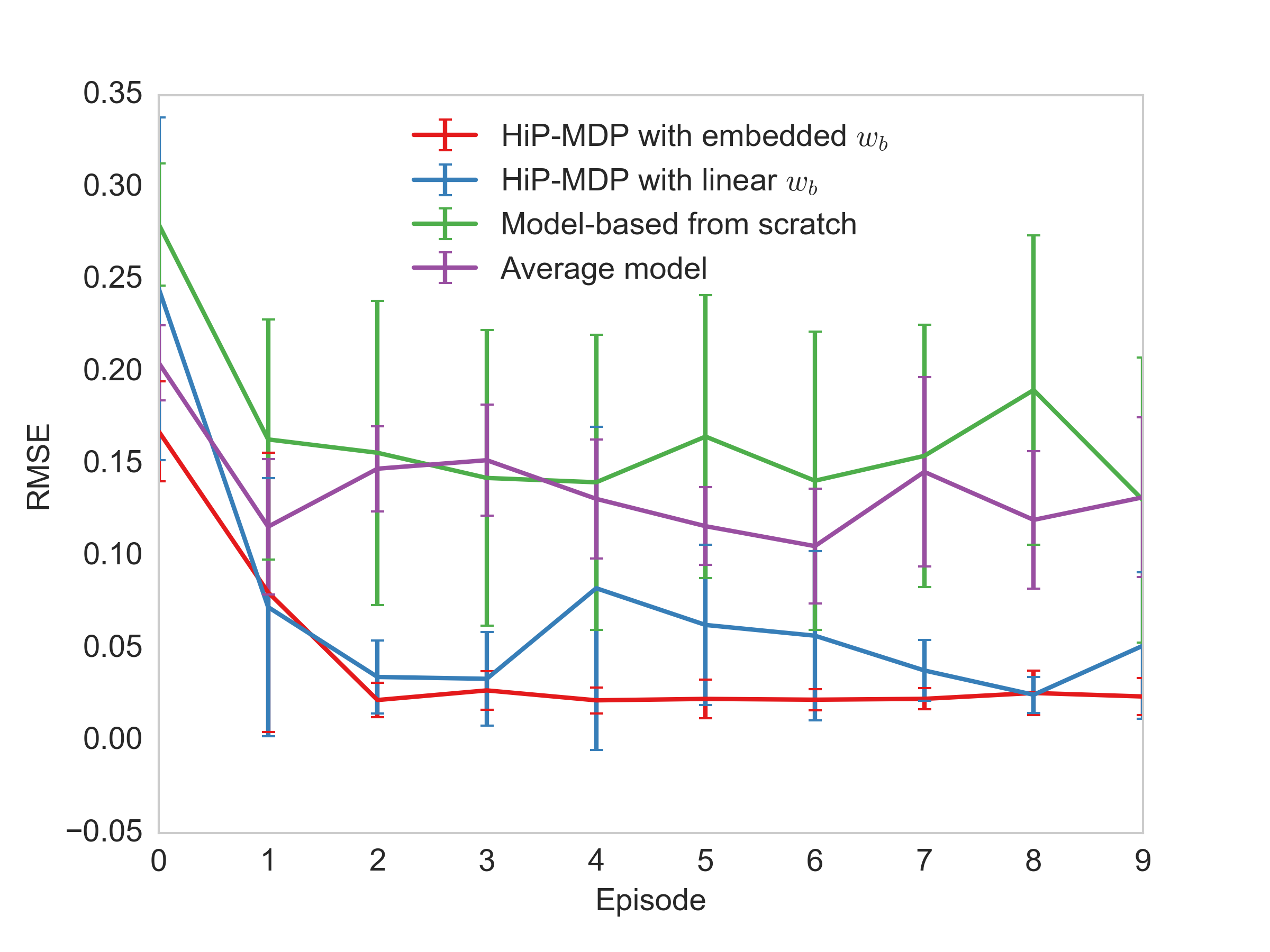
(a) 2D Toy Domain $\left[\mathcal{S}\in\mathbb{R}^{2}\right]$

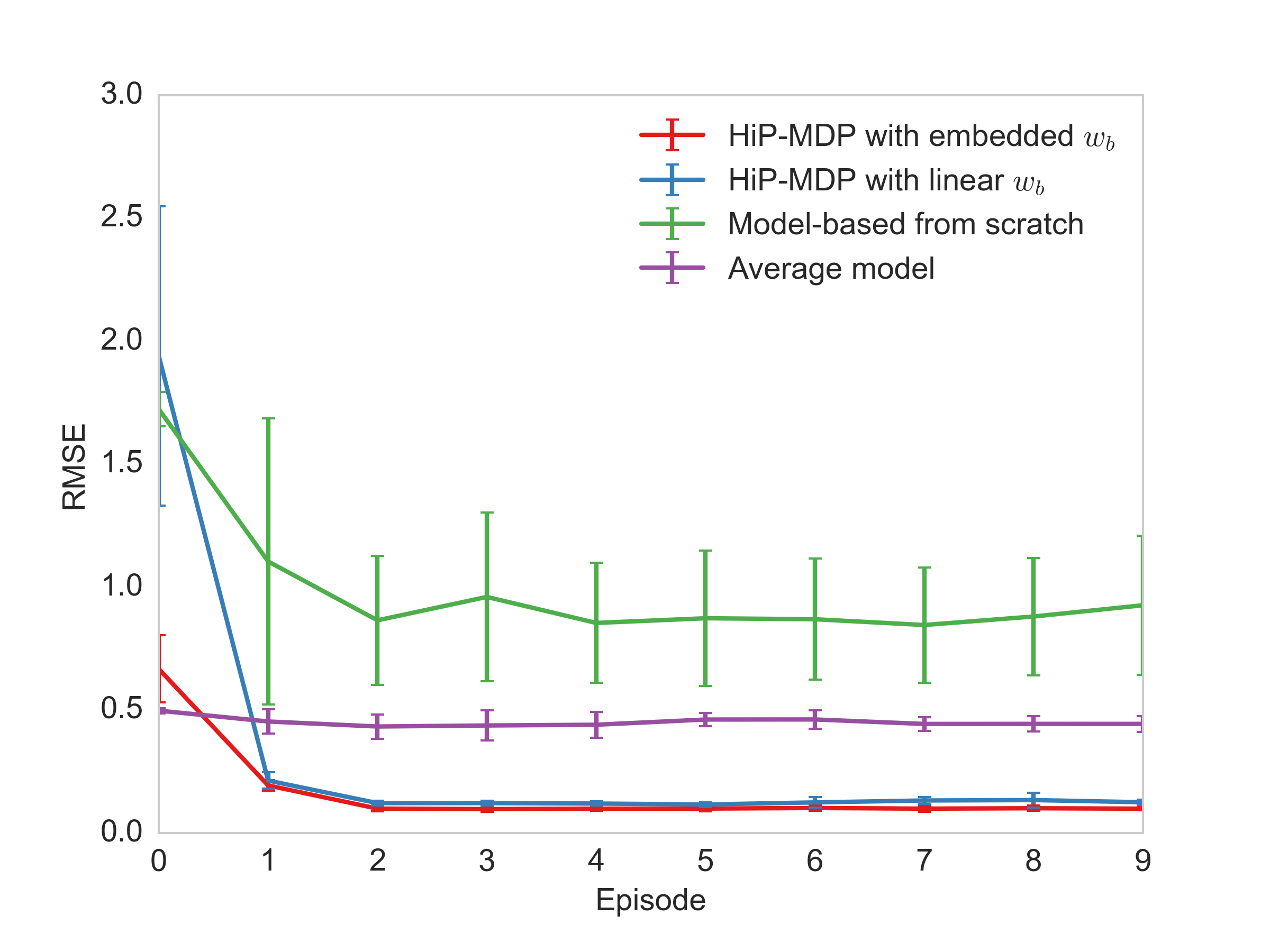
(b) HIV Treatment domain $\left[\mathcal{S}\in\mathbb{R}^{6}\right]$

Figure 6: Comparison of HiP-MDP transition model accuracy with the transition models trained for the baselines presented in Sec. 5

.

The superior predictive performance of the two models that learn and utilize a latent estimate of the underlying dynamics of the environment reinforces the intent of the HiP-MDP as a latent variable model. That is, by estimating and employing a latent estimate of the environment, one may robustly transfer trained transition models to previously unseen instances. Further, as is shown across both domains represented in Fig. 6, the BNN with the latent parametrization embedded with the input is more reliably accurate over the duration the model interacts with a new environment. This is because the HiP-MDP with embedded latent parameters can model nonlinear interactions between the latent parameters and the state and the HiPMDP with linear latent parameters cannot. Moreover, the 2D navigation domain was constructed such that the true transition function is a nonlinear function of the latent parameter and the state. Therefore, the most accurate predictions can only be made with an approximate transition function that can model those nonlinear interactions. Hence, the 2D navigation domain demonstrates the importance of embedding the latent parameters $w_{b}$ with the input of the transition model.

Appendix B Experimental Domains

This section outlines the nonlinear dynamical systems that define the experimental domains investigated in Sec. 5. Here we outline the equations of motion, the hidden parameters dictating the dynamics of that motion, and the procedures used to perturb those parameters to produce subtle variations in the environmental dynamics. Other domain specific settings such as the length of an episode are also presented.

B.1 2D Navigation Domain

As was presented in Sec. 3 the transition dynamics of the 2D navigation domain follow:

$$\Delta x =(-1)^{\theta_{b}}c\big{(}a_{x}-(1-\theta_{b})\beta\sqrt{(x+1.5)^{2}+(y+1.5)^{2}}\big{)}$$

$$\Delta y =(-1)^{\theta_{b}}c\big{(}a_{y}-\theta_{b}\beta\sqrt{(x+1.5)^{2}+(y+1.5)^{2}}\big{)}$$

$$a_{x} =\begin{cases}1&a\in\{E,W\}\\ 0&\text{otherwise}\end{cases}$$

$$a_{y} =\begin{cases}1&a\in\{N,S\}\\ 0&\text{otherwise}\end{cases}$$

Where $c=0.3$ and $\beta=0.23$ are hyperparameters that restrict the agent’s movement either laterally or vertically, depending on the hidden parameter $\theta_{b}$. In this domain, this hidden parameter is simply a binary choice $\left(\theta_{b}\in\{0,1\}\right)$ between the two classes of agent (“blue” or “red”). This force, used to counteract, or accentuate, certain actions of the agent is scaled nonlinearly by the distance the agent moves away from the center of the region of origin.

The agent accumulates a small negative reward (-0.1) for each step taken, a large penalty (-5) if the agent hits a wall or attempts to cross into the goal region over the wrong boundary. The agent receives a substantial reward (1000) once it successfully navigates to the goal region over the correct boundary. This value was purposefully set to be large so as to encourage the agent to more rapidly enter the goal region and move against the force pushing the agent away from the goal region.

At the initialization of a new episode, the class of the agent is chosen with uniform probability and the starting state of the agent is randomly chosen to lie in the region $[-1.75,-1.25]^{2}$.

B.2 Acrobot

The acrobot domain [42] is dictated by the following dynamical system evolving the state parameters $s=\left[\theta_{1},\theta_{2},\dot{\theta}_{1},\dot{\theta}_{2}\right]$:

$$\ddot{\theta}_{1} =-d_{1}^{-1}(d_{2}\ddot{\theta}_{2}+\phi_{1})$$

$$\ddot{\theta}_{2} =\left(m_{2}l_{c2}^{2}+I_{2}-\frac{d_{2}^{2}}{d_{1}}\right)^{-1}\left(\tau+\frac{d_{2}}{d_{1}}\phi_{1}-m_{2}l_{1}l_{c2}\dot{\theta}_{1}^{2}\sin\theta_{2}-\phi_{2}\right)$$

$$d_{1} =m_{1}l_{c1}^{2}+m_{2}(l_{1}^{2}+l_{c2}^{2}+2l_{1}l_{c2}\cos\theta_{2})+I_{1}+I_{2}$$

$$d_{2} =m_{2}(l_{c2}^{2}+l_{1}l_{c2}\cos\theta_{2})+I_{2}$$

$$\phi_{1} =-m_{2}l_{1}l_{c2}\dot{\theta}_{2}^{2}\sin\theta_{2}-2m_{2}l_{1}l_{c2}\dot{\theta}_{2}\dot{\theta}_{1}\sin\theta_{2}+(m_{1}l_{c1}+m_{2}l_{1})g\cos(\theta_{1}-\pi/2)+phi_{2}$$

$$\phi_{2} =m_{2}l_{c2}g\cos(\theta_{1}+\theta_{2}-\pi/2).$$

With reward function $R(s,a)=-0.05\left(\left[-l_{1}\cos(\theta_{1})-l_{2}\cos(\theta_{1}+\theta_{2})\right]-l_{1}\right)^{2}$ if the foot of the pendulum has not exceeded the goal height. If it has, then $R(s,a)=10$ and the episode ends. The hyperparameter settings are $l_{c1}=l_{c2}=0.5$ (lengths to center of mass of links), $I_{1}=I_{2}=1$ (moments of inertia of links) and $g=9.8$ (gravity). The hidden parameters $\theta_{b}$ are the lengths and masses of the two links $(l_{1},l_{2},m_{1},m_{2})$ all set to 1 initially. In order to observe varied dynamics from this system we perturb $\theta_{b}$ by adding Gaussian ($\mathcal{N}(0,0.25)$) noise to each parameter independently at the initialization of a new instance. The possible state values for the angular velocities of the pendulum are constrained to $\dot{\theta}_{1}\in\left[-4\pi,4\pi\right]$ and $\dot{\theta}_{2}\in\left[-9\pi,9\pi\right]$.

At the initialization of a new episode the agent’s state is initialized to $s=(0,0,0,0)$ and perturbed by some small uniformly distributed noise in each dimension. The agent is then free to apply torques to the hinge, until it raises the foot of the pendulum above the goal height or after 400 time steps.

B.3 HIV Treatment

The dynamical system used to simulate a patient’s response to HIV treatments was formulated in [1]. The equations are highly nonlinear in the parameters and are used to track the evolution of six core markers used to infer a patient’s overall health. These markers are, the viral load ($V$), the number of healthy and infected CD4⁺ T-lymphocytes ($T_{1}$ and $T^{*}_{1}$, respectively), the number of healthy and infected macrophages ($T_{2}$ and $T^{*}_{2}$, respectively), and the number of HIV-specific cytotoxic T-cells ($E$). Thus, $s=(V,T_{1},T_{2},T_{1}^{*},T_{2}^{*},E)$. The system of equations is defined as:

$$\dot{T}_{1} =\lambda_{1}-d_{1}T_{1}-(1-\epsilon_{1})k_{1}VT_{1}$$

$$\dot{T}_{2} =\lambda_{2}-d_{2}T_{2}-(1-f\epsilon_{1})k_{2}VT_{2}$$

$$\dot{T}^{*}_{1} =(1-\epsilon_{1})k_{1}VT_{1}-\delta T_{1}^{*}-m_{1}ET_{2}^{*}$$

$$\dot{T}^{*}_{2} =(1-\epsilon_{2})N_{T}\delta(T_{1}^{*}+T_{2}^{*})-cV-[(1-\epsilon_{1})\rho_{1}k_{1}T_{1}+(1-f\epsilon_{1})\rho_{2}k_{2}T_{2}]V$$

$$\dot{E} =\lambda_{E}+\frac{b_{E}(T_{1}^{*}+T_{2}^{*})}{(T_{1}^{*}+T_{2}^{*})+K_{b}}E-\frac{d_{E}(T_{1}^{*}+T_{2}^{*})}{(T_{1}^{*}+T_{2}^{*})+K_{d}}E-\delta_{E}E.$$

With reward function $R(s,a)=-0.1V-2e^{4}\epsilon_{1}^{2}-2e^{3}\epsilon_{2}^{2}+1e^{3}E$, where $\epsilon_{1},\epsilon_{2}$ are treatment specific parameters, selected by the prescribed action.

The hidden parameters $\theta_{b}$ with their baseline settings [1] are shown in Fig. 7.

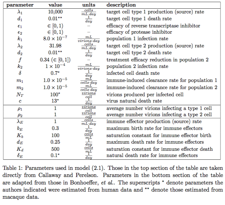
Figure 7: The hidden parameters that dictate the system dynamics of the HIV Treatment domain with their baseline values. Table courtesy of Adams et al. [1].

As was done with the Acrobot at the initialization of a new instance, these hidden parameters are perturbed with by some Gaussian noise ($\mathcal{N}(\theta_{b,i},0.25)$) each parameter independently. These perturbations were applied naively and at times would cause the dynamical system to lose stability or otherwise provide non-physical behavior. We filter out such instantiations of the domain and deploy the HiP-MDP on well-behaved and controllable versions of this dynamical system.

At the initialization of a new episode the agent is started at an unhealthy steady state

$$s=[163573,5,11945,46,63919,24],$$

where the viral load and number of infected cells are much higher than the number of virus fighting T-cells. An episode is characterized by 200 time steps where, dynamically, one time step is equivalent to 5 days. At each 5 day interval, the patient’s state is taken and is prescribed a treatment until the treatment period (or 1000 days) has been completed.

Appendix C Experiment Specifications

C.1 Bayesian neural network

HiP-MDP architecture

For all domains, we model the dynamics using a feed-forward BNN. For the toy example, we used 3 fully connected hidden layers with 25 hidden units each, and for the acrobot and HIV domains, we used 2 fully connected hidden layers with 32 units each. We used rectifier activation functions, $\phi(x)=\max(x,0)$, on each hidden layer, and the identity activation function, $\phi(x)=x$, on the output layer. For the HiP-MDP with embedded $w_{b}$, the input to the BNN is a vector of length $D+|A|+|w_{b}|$ consisting of the state $s$, a one-hot encoding of the action $a$, and the latent embedding $w_{b}$. The BNN architecture for the the HiP-MDP with linear $w_{b}$ uses a different input layer and output layer. The BNN input does not include the latent parameters. Rather the BNN output, $\hat{T}^{(BNN)}(s,a)$ is a matrix of shape $|w_{b}|\times D$. The next state is computed as $s^{\prime}=w_{b}^{T}\hat{T}^{(BNN)}(s,a)$. In all experiments, the BNN output is the state difference $(s^{\prime}-s)$ rather than the next state $s^{\prime}$.

Hyperparameters and Training

For all domains, we put zero mean priors on the random input noise and the network weights with variances of 1.0 and $e^{-10}$, respectively, following the procedure used by Hernández-Lobato et al. [22]. In our experiments, we found the BNN performed best when initialized with a small prior variance on the network weights that increases over training, rather than using a large prior variance. Following Hernández-Lobato et al. [22], we learn the network parameters by minimizing the $\alpha$-divergence using ADAM with $\alpha=0.5$ for acrobot and the toy example and $\alpha=0.45$ for the HIV domain. In each update to the BNN, we performed 100 epochs of ADAM, where in each epoch we sampled 160 transitions from a prioritized experience buffer and divided those transitions into mini batches of size 32. We used a learning rate of $2.5\text{\sc{e}-}{4}$ for HIV and acrobot and learning rate of $5\text{\sc{e}-}{5}$ for the toy example.

The BNN and latent parameters were learned from a batch of transition data gathered from multiple instances across 500 episodes per instance. For the toy example, acrobot, and HIV, we use data from 2, 8, and 5 instances, respectively. For HIV, we found performance improved by standardizing the observed states to have zero mean, unit variance.

C.2 Latent Parameters

For all domains, we used $|w_{b}|=5$ latent parameters. The latent parameters were updated using the same update procedure as for updating the BNN network parameters (except with the BNN network parameters held fixed) with a learning rate of $5\text{\sc{e}-}{4}$.

C.3 Deep Q-Network

To learn a policy for a new task instance, we use a Double Deep Q Network with two full connected hidden layers with 256 and 512 hidden units, respectively. Rectifier activation functions are used for the hidden layers and the identity function is used on for the output layer. For all domains, we update the primary network weights every $N_{\pi}=10$ time steps using ADAM with a learning rate of $5\text{\sc{e}-}{4}$, and slowly update the target network to mirror the primary network with a rate of $\tau=0.005$. Additionally, we clip gradients such that the L2-norm is less than 2.5. We use an $\epsilon$-greedy policy starting with $\epsilon=1.0$ and decaying $\epsilon$ after each episode (each real episode for the model-free approach and each approximated episode for the model-based approaches) with a rate of $0.995$.

In model-based approaches, we found that the DQN learns more robust policies (both on the BNN approximate dynamics and the real environment) from training exclusively off the approximated transitions of the BNN. After training the BNN off the first episode, we train the DQN using an initial batch of $N_{f}=500$ approximated episodes generated using the BNN.

C.4 Prioritized Experience Replay Buffers

We used a TD-error-based prioritized experience replay buffer [38] to store experiences used to train the DQN. For model-based approaches, we used a separate squared-error-based prioritized buffer to store experiences used to train the BNN and learn the latent parameterization. Each prioritized buffer was large enough to store all experiences. We used a prioritization exponent of 0.2 and an importance sampling exponent of 0.1.

Appendix D Long run demonstration of policy learning

We demonstrate that all benchmark methods used learn good control policies for new, unique instances of the acrobot domain (Figure 8(a)) and the HIV treatment domain (Figure 8(b)) with a sufficient number of training episodes. However, in terms of policy learning efficiency and proficiency, comparing the performance of the HiP-MDP with the benchmark over the first 10 episodes is instructive—as presented the Experiments section of the main paper. This format emphasizes the immediate returns of using the embedded latent parameters to transfer previously learned information when encountering a new instance of a task.

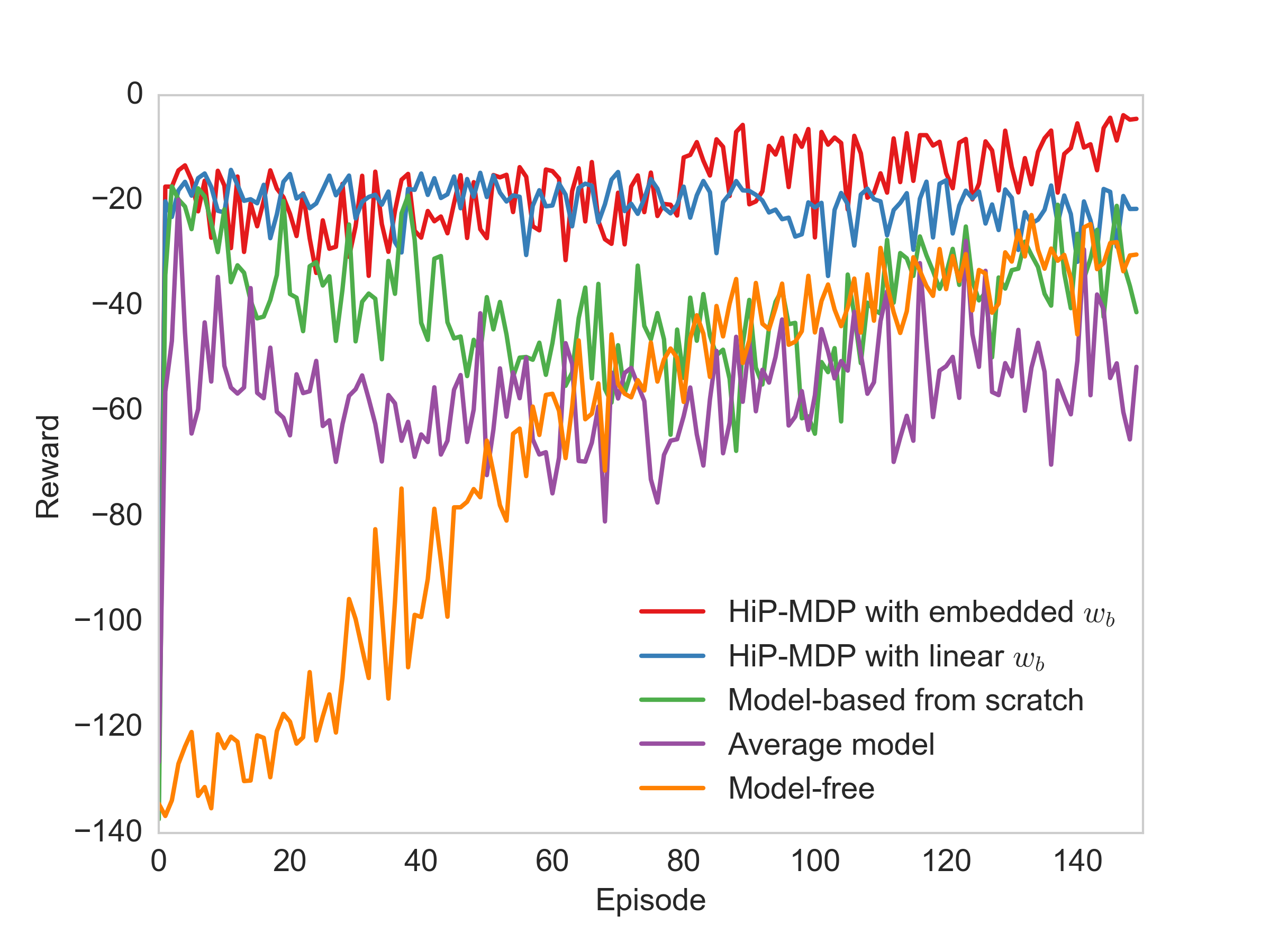
(a) Acrobot

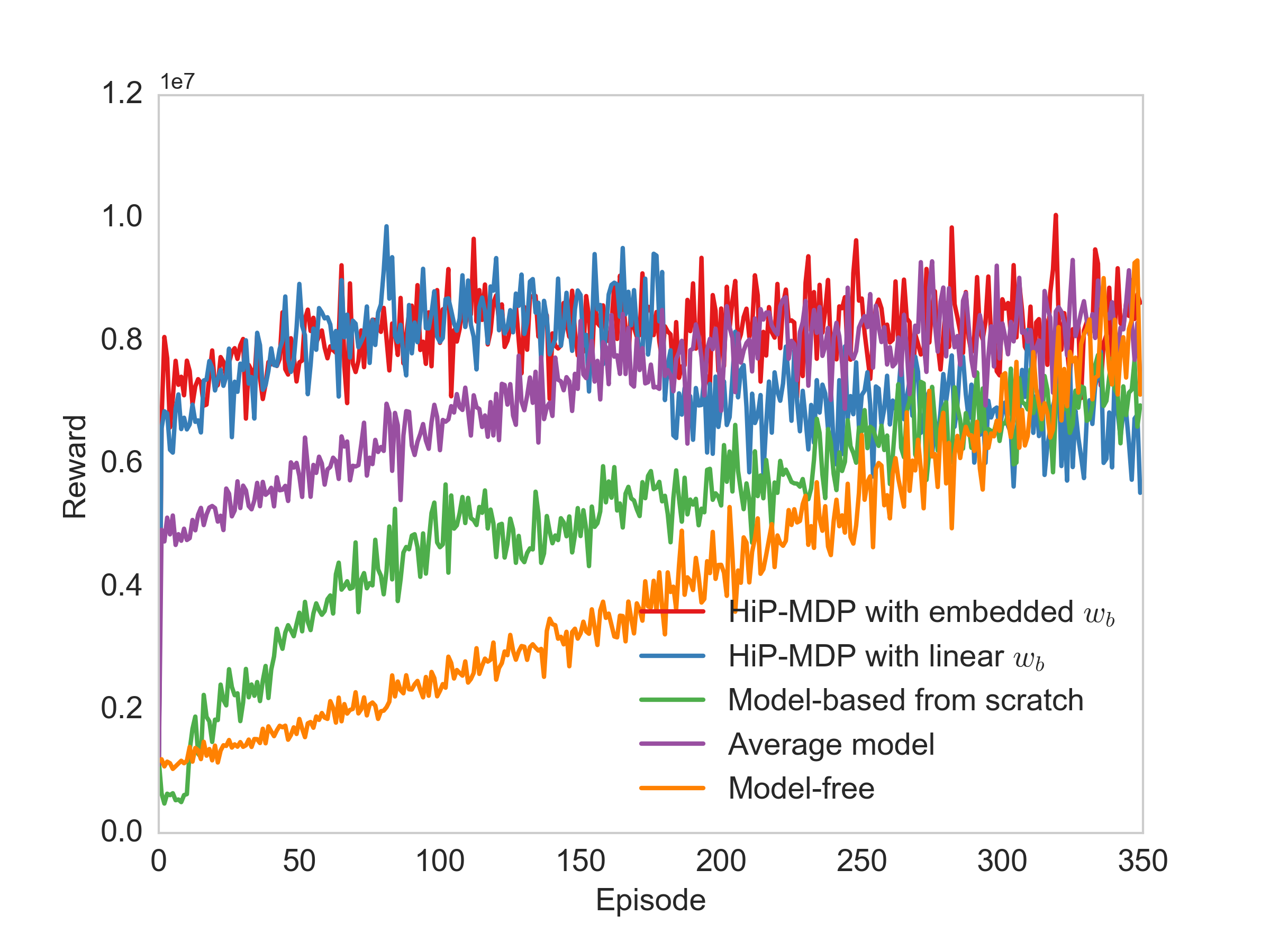
(b) HIV Treatment

Figure 8: A comparison of learning a policy for a new task instance $b$ using the HiP-MDP versus four benchmarks over more episodes. The mean reward for each episode over 5 runs is shown for each benchmark. The error bars are omitted to show the results clearly.

References

- Adams et al. [2004] BM Adams, HT Banks, H Kwon, and HT Tran. Dynamic multidrug therapies for HIV: optimal and STI control approaches. Mathematical Biosciences and Engineering, pages 223–241, 2004.
- Alvarez et al. [2012] MA Alvarez, L Rosasco, ND Lawrence, et al. Kernels for vector-valued functions: A review. Foundations and Trends® in Machine Learning, 4(3):195–266, 2012.
- Bai et al. [2013] H Bai, D Hsu, and W S Lee. Planning how to learn. In Robotics and Automation, International Conference on, pages 2853–2859. IEEE, 2013.
- Blundell et al. [2015] C Blundell, J Cornebise, K Kavukcuoglu, and D Wierstra. Weight uncertainty in neural networks. In Proceedings of The 32nd International Conference on Machine Learning, pages 1613–1622, 2015.
- Bonilla et al. [2008] EV Bonilla, KM Chai, and CK Williams. Multi-task Gaussian process prediction. In Advances in Neural Information Processing Systems, volume 20, pages 153–160, 2008.
- Brunskill and Li [2013] E Brunskill and L Li. Sample complexity of multi-task reinforcement learning. arXiv preprint arXiv:1309.6821, 2013.
- Caruana [1998] R Caruana. Multitask learning. In Learning to learn, pages 95–133. Springer, 1998.
- Chen et al. [2016] M Chen, E Frazzoli, D Hsu, and WS Lee. POMDP-lite for robust robot planning under uncertainty. In Robotics and Automation, International Conference on, pages 5427–5433. IEEE, 2016.
- Deisenroth and Rasmussen [2011] MP Deisenroth and CE Rasmussen. PILCO: a model-based and data-efficient approach to policy search. In In Proceedings of the International Conference on Machine Learning, 2011.
- Delhaisse et al. [2017] B Delhaisse, D Esteban, L Rozo, and D Caldwell. Transfer learning of shared latent spaces between robots with similar kinematic structure. In Neural Networks, International Joint Conference on. IEEE, 2017.
- Depeweg et al. [2017a] S Depeweg, JM Hernández-Lobato, F Doshi-Velez, and S Udluft. Learning and policy search in stochastic dynamical systems with Bayesian neural networks. In International Conference on Learning Representations, 2017a.
- Depeweg et al. [2017b] S Depeweg, JM Hernández-Lobato, F Doshi-Velez, and S Udluft. Uncertainty decomposition in bayesian neural networks with latent variables. arXiv preprint arXiv:1706.08495, 2017b.
- Dietrich and Newsam [1997] CR Dietrich and GN Newsam. Fast and exact simulation of stationary gaussian processes through circulant embedding of the covariance matrix. SIAM Journal on Scientific Computing, 18(4):1088–1107, 1997.
- Doshi-Velez and Konidaris [2016] F Doshi-Velez and G Konidaris. Hidden parameter Markov Decision Processes: a semiparametric regression approach for discovering latent task parametrizations. In Proceedings of the Twenty-Fifth International Joint Conference on Artificial Intelligence, volume 25, pages 1432–1440, 2016.
- Ernst et al. [2006] D Ernst, G Stan, J Goncalves, and L Wehenkel. Clinical data based optimal STI strategies for HIV: a reinforcement learning approach. In Proceedings of the 45th IEEE Conference on Decision and Control, 2006.
- Fern and Tadepalli [2010] A Fern and P Tadepalli. A computational decision theory for interactive assistants. In Advances in Neural Information Processing Systems, pages 577–585, 2010.
- Gal and Ghahramani [2016] Y Gal and Z Ghahramani. Dropout as a Bayesian approximation: representing model uncertainty in deep learning. In Proceedings of the 33rd International Conference on Machine Learning, 2016.
- Gal et al. [2016] Y Gal, R McAllister, and CE Rasmussen. Improving PILCO with Bayesian neural network dynamics models. In Data-Efficient Machine Learning workshop, ICML, 2016.
- Genton et al. [2015] MG Genton, W Kleiber, et al. Cross-covariance functions for multivariate geostatistics. Statistical Science, 30(2):147–163, 2015.
- Gupta et al. [2017] A Gupta, C Devin, Y Liu, P Abbeel, and S Levine. Learning invariant feature spaces to transfer skills with reinforcement learning. In International Conference on Learning Representations, 2017.
- Hasselt et al. [2016] H van Hasselt, A Guez, and D Silver. Deep reinforcement learning with double Q-learning. In Proceedings of the Thirtieth AAAI Conference on Artificial Intelligence, pages 2094–2100. AAAI Press, 2016.
- Hernández-Lobato et al. [2016] JM Hernández-Lobato, Y Li, M Rowland, D Hernández-Lobato, T Bui, and RE Turner. Black-box -divergence minimization. In Proceedings of The 33rd International Conference on Machine Learning, 2016.
- Jaques et al. [2015] N Jaques, S Taylor, A Sano, and R Picard. Multi-task, multi-kernel learning for estimating individual wellbeing. In Proc. NIPS Workshop on Multimodal Machine Learning, 2015.
- Kaelbling et al. [1998] LP Kaelbling, ML Littman, and AR Cassandra. Planning and acting in partially observable stochastic domains. Artificial intelligence, 101(1):99–134, 1998.
- Kendall and Gal [2017] A Kendall and Y Gal. What uncertainties do we need in bayesian deep learning for computer vision? arXiv preprint arXiv:1703.04977, 2017.
- Kingma and Ba [2015] D Kingma and J Ba. Adam: A method for stochastic optimization. In International Conference on Learning Representations, 2015.
- MacKay [1992] D JC MacKay. A practical Bayesian framework for backpropagation networks. Neural computation, 4(3):448–472, 1992.
- Marivate et al. [2014] VN Marivate, J Chemali, E Brunskill, and M Littman. Quantifying uncertainty in batch personalized sequential decision making. In Workshops at the Twenty-Eighth AAAI Conference on Artificial Intelligence, 2014.
- Mnih et al. [2015] V Mnih, K Kavukcuoglu, D Silver, A A Rusu, J Veness, M G Bellemare, A Graves, M Riedmiller, A K Fidjeland, G Ostrovski, et al. Human-level control through deep reinforcement learning. Nature, 518(7540):529–533, 2015.
- Moerland et al. [2017] TM Moerland, J Broekens, and CM Jonker. Learning multimodal transition dynamics for model-based reinforcement learning. arXiv preprint arXiv:1705.00470, 2017.
- Moore and Atkeson [1993] AW Moore and CG Atkeson. Prioritized sweeping: reinforcement learning with less data and less time. Machine learning, 13(1):103–130, 1993.
- Moore et al. [2014] BL Moore, LD Pyeatt, V Kulkarni, P Panousis, K Padrez, and AG Doufas. Reinforcement learning for closed-loop propofol anesthesia: a study in human volunteers. Journal of Machine Learning Research, 15(1):655–696, 2014.
- Neal [1992] RM Neal. Bayesian training of backpropagation networks by the hybrid Monte carlo method. Technical report, Citeseer, 1992.
- Quiñonero-Candela and Rasmussen [2005] J Quiñonero-Candela and CE Rasmussen. A unifying view of sparse approximate gaussian process regression. Journal of Machine Learning Research, 6(Dec):1939–1959, 2005.
- Rasmussen and Kuss [2003] CE Rasmussen and M Kuss. Gaussian processes in reinforcement learning. In Advances in Neural Information Processing Systems, volume 15, 2003.
- Rasmussen and Williams [2006] CE Rasmussen and CKI Williams. Gaussian processes for machine learning. MIT Press, Cambridge, 2006.
- Rosman et al. [2016] B Rosman, M Hawasly, and S Ramamoorthy. Bayesian policy reuse. Machine Learning, 104(1):99–127, 2016.
- Schaul et al. [2016] T Schaul, J Quan, I Antonoglou, and D Silver. Prioritized experience replay. In International Conference on Learning Representations, 2016.
- Schulam and Saria [2016] P Schulam and S Saria. Integrative analysis using coupled latent variable models for individualizing prognoses. Journal of Machine Learning Research, 17:1–35, 2016.
- Shortreed et al. [2011] SM Shortreed, E Laber, DJ Lizotte, TS Stroup, J Pineau, and SA Murphy. Informing sequential clinical decision-making through reinforcement learning: an empirical study. Machine learning, 84(1-2):109–136, 2011.
- Snelson and Ghahramani [2006] E Snelson and Z Ghahramani. Sparse gaussian processes using pseudo-inputs. In Advances in Neural Information Processing Systems, pages 1257–1264, 2006.
- Sutton and Barto [1998] R Sutton and A Barto. Reinforcement learning: an introduction, volume 1. MIT Press, Cambridge, 1998.
- Taylor and Stone [2009] ME Taylor and P Stone. Transfer learning for reinforcement learning domains: a survey. Journal of Machine Learning Research, 10(Jul):1633–1685, 2009.
- [44] M Tenenbaum, A Fern, L Getoor, M Littman, V Manasinghka, S Natarajan, D Page, J Shrager, Y Singer, and P Tadepalli. Personalizing cancer therapy via machine learning.
- Williams and Young [2006] JD Williams and S Young. Scaling POMDPs for dialog management with composite summary point-based value iteration (CSPBVI). In AAAI Workshop on Statistical and Empirical Approaches for Spoken Dialogue Systems, pages 37–42, 2006.