Gravito-turbulence and the excitation of small-scale parametric instability in astrophysical discs

Abstract

Young protoplanetary discs and the outer radii of active galactic nucleii may be subject to gravitational instability and, as a consequence, fall into a ‘gravitoturbulent’ state. While in this state, appreciable angular momentum can be transported. Alternatively, the gas may collapse into bound clumps, the progenitors of planets or stars. In this paper, we numerically characterize the properties of 3D gravitoturbulence, focussing especially on its dependence on numerical parameters (resolution, domain size) and its excitation of small-scale dynamics. Via a survey of vertically stratified shearing box simulations with PLUTO and RODEO, we find (a) evidence that certain gravitoturbulent properties are independent of horizontal box size only when the box is larger than $\simeq 40H$, where $H$ is the height scale, (b) at high resolution, small-scale isotropic turbulence appears off the midplane around $z\simeq 0.5-1H_{0}$, and (c) this small-scale dynamics results from a parametric instability, involving the coupling of inertial waves with a large-scale axisymmetric epicyclic mode. This mode oscillates at a frequency close to $\Omega$ and is naturally excited by gravito-turbulence, via a nonlinear process to be determined. The small-scale turbulence we uncover has potential implications for a wide range of disc physics, e.g. turbulent saturation levels, fragmentation, turbulent mixing, and dust settling.

1 Introduction

Gravitational instability (GI) attacks gaseous accretion disks that are sufficiently cold and massive, as might be the case in the early stages of a protoplanetary (PP) disk’s life (e.g. Durisen et al., 2007), or beyond roughly 0.01 pc in active galactic nucleii (AGN, e.g. Shlosman & Begelman, 1987). Recent observations of wide-orbit planets and spiral structure have fueled ongoing interest in GI within the PP disk context (Fukagawa et al., 2013; Christiaens et al., 2014; Kalas et al., 2008), while indications of transonic turbulence from maser emission, and the long-standing questions of disk truncation, star formation, and the sustenance of high accretion rates motivate its study in AGN (e.g Wallin et al., 1998; Goodman, 2003).

The critical parameter that sets the onset of the gravitational instability is the Toomre $Q$ (Toomre, 1964),

$$Q=\dfrac{c_{s}\kappa}{\pi G\Sigma_{0}},$$ (1)

where $c_{s}$ is the sound speed, $\kappa$ the epicyclic frequency, and $\Sigma_{0}$ the background surface density. In a razor thin disk, linear axisymmetric disturbances are unstable when $Q<1$, but nonlinear non-axisymmetric instability can occur for $Q\gtrsim 1$. If the cooling is relatively inefficient, simulations show that the disk falls into a gravitoturbulent state comprised of a disordered field of spiral density waves that transports significant angular momentum (Gammie, 2001; Rice et al., 2014). On the other hand, if the cooling is overly efficient the disc fragments into dense clumps that may be the precursors of gaseous giant planets or stars (Cameron, 1978; Boss, 1997).

Most numerical work is undertaken in a global setting, and indeed the characteristic lengthscales of the gravitoturbulent spiral waves is generally large-scale. But owing to inadequate resolution, global models struggle to describe dynamics on scales of order the disk thickness $H$ or less, which are important for turbulent mixing, dust settling, and (possibly) fragmentation. Local 3D shearing-box models are better suited for exploring these processes, though this is a research direction that has been neglected, for the most part, in the modelling of GI in disks. Recently, Shi & Chiang (2014) presented 3D local box simulations that showed that the gravitoturbulent state failed to exhibit appreciable structure on scales less than $H$ (see also Hirose & Shi (2017)). However, their resolution (a maximum $8$ points per $H$) was probably too low to properly characterise any small-scale features. In particular, it was unclear if their results had converged with resolution. While the density waves are expected to exhibit little vertical structure (being essentially f-modes, Ogilvie, 1998), they are potentially vulnerable to parasitic instabilities relying on a parametric resonance between small-scale inertial modes (Fromang & Papaloizou, 2007; Bae et al., 2016b). An open question is whether this secondary instability also operates in gravitoturbulence, and what influence it has on the properties of the spiral waves.

To address this issue, we performed 3D local shearing box simulations of gravito-turbulent discs, with vertical stratification and an ideal gas law. Two different codes were used, PLUTO and RODEO, and these were subject to a number of numerical checks, so as to confirm the trustworthiness of our results. Our main finding is that vigorous and isotropic small-scale turbulence develops slightly off the disk midplane and disturbs the spiral waves generated by GI. The small-scale turbulence is obtained only in high resolution runs (at least 20 cells per disc height scale), and thus has not been captured in previous under-resolved simulations: either SPH or grid-based, local or global.

We are persuaded that the small-scale activity is excited via a 3D parametric instability that couples pairs of inertial waves and a large-scale axisymmetric epicyclic oscillation. Unstable inertial waves develop in the midplane but break nonlinearly at a higher altitude, resulting in helical, incompressible and non-axisymmetric motions around $z=0.5-1\,H$. We also consider the merits of the Kelvin-Helmholtz instability, vertical splashing caused by colliding density wakes, and the preferential breaking of wakes in the disk atmosphere, but find each in conflict with our numerical diagnostics. We discuss the emergence of the large-scale epicyclic oscillations (upon which the parametric instability feeds), and speculate on their importance to both the subcritical transition to GI turbulence and its continued sustenance.

The structure of the paper is as follows: First, in Section 2, we introduce the basic equations of the problem and discuss our numerical setup. In Section 3 we study the dependence of the 3D gravito-turbulent state on the numerical parameters, in particular the grid resolution and box size. We show evidence that turbulent quantities are converged with horizontal box sizes $L_{x}=L_{y}$ if $L_{x}\gtrsim 40H_{0}$. In Section 4, we characterise the small-scale dynamics and the large-scale axisymmetric oscillation in Fourier space. In Section 5, we analyse the nature of the small-scale parasitic turbulence and show how it may result from a parametric instability. Finally, in Section 6, we discuss the possible implications of our results for disc physics, in particular for turbulent mixing, dust dynamics, and the evolution of magnetic fields.

2 Numerical model

2.1 Governing equations

We assume that the gas orbiting around the central object is ideal, its pressure $P$ and density $\rho$ related by $\gamma P=\rho c_{s}^{2}$, where $c_{s}$ is the sound speed and $\gamma$ the ratio of specific heats. The pressure is related to internal energy $U$ by $P=(\gamma-1)U$. We neglect molecular viscosity. We treat a local Cartesian model of an accretion disk (the shearing sheet; Goldreich & Lynden-Bell, 1965). In this model, the axisymmetric differential rotation is approximated locally by a linear shear flow and a uniform rotation $\bm{\Omega}=\Omega\,\mathbf{e}_{z}$, with $S=(3/2)\,\Omega$ for a Keplerian equilibrium. We denote by $(x,y,z)$ the shearwise, streamwise and spanwise directions, corresponding to radius, azimuth, and the vertical. The shearing sheet approximation works best when the disk’s angular thickness is small (see for e.g. Balbus & Papaloizou, 1999), and thus PP disks are only marginally covered by the model. In fact, for our largest domains it is difficult to justify the shearing box. AGN disks, being much thinner, are better described. We persist with the shearing sheet, however, as it provides a well-defined platform and the superior resolution needed to probe the smaller scales.

The evolution of density ${\rho}$, total velocity field $\mathbf{v}$, and internal energy $U$ follows:

$$\dfrac{\partial\rho}{\partial t}+\nabla\cdot\left(\rho\mathbf{v}\right)=0,$$ (2)

$$\frac{\partial{\mathbf{v}}}{\partial{t}}+\mathbf{v}\cdot\mathbf{\nabla v}+2\bm{\Omega}\times\mathbf{v}=-\nabla\Phi-\dfrac{\mathbf{\nabla}{P}}{\rho},$$ (3)

$$\dfrac{\partial U}{\partial t}+\nabla\cdot(U\mathbf{v})=-P\nabla\cdot\mathbf{v}-\dfrac{U}{\tau_{c}}.$$ (4)

The total velocity field may be decomposed into

$$\mathbf{v}=-Sx\,\mathbf{e}_{y}+\mathbf{u},$$ (5)

where $\mathbf{u}$ is the perturbed velocity field. The potential $\Phi$ is the sum of the tidal potential induced by the central object in the local frame, $\Phi_{c}=\frac{1}{2}\Omega^{2}z^{2}-\frac{3}{2}\Omega^{2}\,x^{2}$, and the gravitational potential induced by the disc itself, $\Phi_{s}$, which obeys the Poisson equation:

$$\nabla^{2}\Phi_{s}=4\pi G\rho.$$ (6)

In the energy equation (4), the cooling varies linearly with $U$ with a typical timescale $\tau_{c}$ referred to as the ‘cooling time’. This prescription is not very realistic but allows us to control the rate of energy loss via a single parameter. We neglect thermal conductivity. Finally, $\Omega^{-1}$ defines our unit of time and $H_{0}$, the initial disc scale-height (defined below), our reference unit of length.

2.2 Disc background equilibrium

When $\tau_{c}\to\infty$, the governing equations admit an equilibrium state characterised by $\mathbf{u}=0$, and vertical hydrostatic balance. We consider homentropic equilibria, for which the vertical profile is polytropic $P=K\rho^{\gamma}$. Here $K=c_{s_{0}}^{2}/(\gamma\rho_{0}^{\gamma-1})$, with $c_{s_{0}}$ and $\rho_{0}$ denoting the midplane sound speed and density, respectively. The equilibrium equations are

$$K\left[\dfrac{1}{\rho}\dfrac{d\rho^{\gamma}}{dz}\right]+z\Omega^{2}+\dfrac{d\Phi_{s}}{dz}=0,$$ (7)

$$\dfrac{d^{2}\Phi_{s}}{dz^{2}}=4\pi G\rho,$$ (8)

which reduce to an inhomogeneous form of the Emden-Fowler equation. Appendix A gives details on how to solve these equations numerically. These solutions form part of our simulations’ initial condition.

2.3 Numerical methods

2.3.1 Codes

Direct numerical simulations of the three-dimensional flow are performed in the shearing box. The box has a finite domain of size $(L_{x},L_{y},L_{z})$, discretized on a mesh of $(N_{X},N_{Y},N_{Z})$ grid points. For most of the numerical runs, we use the Godunov-based PLUTO code (Mignone et al., 2007), which is well adapted to highly compressible flow and shocks. This scheme uses a conservative finite-volume method that solves the approximate Riemann problem at each inter-cell boundary. It is known to successfully reproduce the behaviour of conserved quantities like mass, momentum, and total energy. The Riemann problem is handled by the HLLC solver which properly describes contact discontinuities and has the advantage of being robust and positivity preserving.

To allow longer time steps and eliminate numerical artifacts at the boundaries, where the background shear flow is often very strong, we use the orbital advection algorithm of PLUTO. It is based on splitting the equation of motion into two parts, the first containing the linear advection operator due to the background Keplerian shear and the second the standard fluxes and source terms. Finally, PLUTO conserves the total energy and so the heat equation is not solved directly as in Eq.(4). Hence the code captures the irreversible heat produced by shocks due to numerical diffusion, consistent with the Rankine-Hugoniot conditions.

In Section 3.5, we compare our results with another code, RODEO, that has previously simulated self-gravitating disc in the 2D shearing box (Paardekooper, 2012). Similar to PLUTO, it is a Godunov-based method but one that relies on the Roe solver (Roe, 1981) to calculate interface fluxes. Second-order accuracy in space and time is achieved through a wave limiting procedure as described, for example, in LeVeque (2002). Most of the results were obtained with the minmod wave limiter (Roe, 1986), although we briefly explore different limiters. One other significant difference with PLUTO is that the RODEO simulations were performed in shearing coordinates, where the usual $y$ coordinate is replaced by $y^{\prime}=y+3/2\Omega tx$. In this way, the use of an orbital advection algorithm is avoided, at the expense of a periodic remap every $\tau_{\mathrm{remap}}$, which, by a clever choice of $\tau_{\mathrm{remap}}$, can be done by shifting an integer number of grid cells in $y$. This procedure therefore does not introduce any numerical diffusion.

2.3.2 Poisson solver

While in RODEO a pure Fourier Poisson solver was used (Koyama & Ostriker, 2009), a different approach was taken in the PLUTO simulations in order to more robustly establish our numerical results. This is explained in this subsection.

To compute the gravitational potential, we take advantage of the shear-periodic boundary conditions. In a similar manner to Riols & Latter (2016), we first shift back the density in $y$ to the time it was last periodic $(t=t_{p})$. Then, for each plane of altitude $z_{k}$, we perform the direct 2D Fourier transform of the density $\rho$ and obtain a vertical profile for each coefficient $\hat{\rho}_{k_{x},k_{y}}(z)$ of its Fourier decomposition, where $k_{x}$ and $k_{y}$ are radial and azimuthal wavenumbers. Using Eq. 6, it is straightforward to show that in Fourier space, the coefficients of the gravitational potential satisfy the Helmholtz equation:

$$\left[\dfrac{d^{2}}{dz^{2}}-k^{2}\right]\hat{\Phi}_{k_{x},k_{y}}(z)=4\pi G\hat{\rho}_{k_{x},k_{y}}(z)$$ (9)

with $k=k_{x}^{2}+k_{y}^{2}$, and $\hat{\Phi}_{k_{x},k_{y}}$ the Fourier transform of the potential. This differential equation is solved in the complex plane by means of a fourth-order finite-difference scheme and a direct inversion method. The discretized system takes the form of a linear problem $\mathsf{AX}=\mathsf{B}$ where $\mathsf{X}$ is a vector representing the discretized potential’s $z-$profile, $\mathsf{A}$ is a penta-diagonal matrix, and $\mathsf{B}$ is a column vector containing the right hand side of Eq. 9 and extra coefficients setting the boundary conditions. We use a fast algorithm involving $O(N_{Z})$ flops to invert the matrix and obtain the discretized coefficents $\hat{\Phi}_{k_{x},k_{y}}(z_{k})$. For each altitude $z_{k}$, we finally compute the inverse Fourier transform of the potential and shift it back to the initial sheared frame. Note that gravitational forces are obtained by computing the derivative of the potential in each direction, using a 4th-order finite-difference method.

In total, the computational cost is of order $O(N\log(N_{X}N_{Y}))$ where $N=N_{X}N_{Y}N_{Z}$, and is hence less expensive than a full 3D Fourier decomposition which would be $O(N\log(N))$. Moreover, methods using vertical Fourier decomposition generally assume periodic or vacuum boundary conditions for the potential. Hence, a correct treatment of self-gravity in these methods requires the addition of two buffer zones of size $L_{z}/2$ on either sides of the box, greatly increasing the numerical workload (Koyama & Ostriker, 2009; Shi & Chiang, 2014). In contrast, our setup can handle any boundary condition without artificially augmenting the vertical domain. The stratified disc equilibria as well as the linear stability of these equilibria have been tested to ensure that our implementation is correct (see Appendices A and B).

2.3.3 Boundary conditions

The shearing box framework implicitly assumes periodic boundary conditions in $y$ and shear-periodic boundary condition in $x$. The most delicate part is to assign suitable vertical boundary conditions. We use the standard outflow conditions for velocity and density fields but compute a hydrostatic balance in the ghost cells for pressure, taking into account the large scale vertical component of the self-gravity (averaged in $x$ and $y$). In this way we significantly reduce the excitation of waves near the boundary (see Fig. 15 in Appendix A).

For the gravitational potential, we impose

$$\dfrac{d}{dz}\hat{\Phi}_{k_{x},k_{y}}(\pm{L_{z}}/{2})=\mp k\hat{\Phi}_{k_{x},k_{y}}(\pm{L_{z}}/{2}).$$ (10)

This condition is an approximation of the Poisson equation in the limit of low density. Finally, we impose a density floor of $10^{-4}\,\Sigma/H_{0}$ which prevents the timestep getting too small because of evacuated regions near the vertical boundaries.

2.4 Simulation setup

2.4.1 Box size and resolution

The axisymmetric linear theory tells us that the fastest growing mode possesses a radial lengthscale of order $H\,Q$ when $Q<1$. Although our simulations focus on the regime $Q\gtrsim 1$, we expect typical lengthscales for spiral waves to be $\gtrsim H$. So in order to obtain good statistical averages of the turbulent properties and ensure that the largest structures remain smaller than the domain size, it is necessary to set $L_{x},\,L_{y}\gg H$. As a compromise between this constraint and numerical feasibility (for sufficient resolution), we employ boxes of intermediate size $L_{x}=L_{y}=20\,H_{0}$, though we explore larger sizes in Section 3.2.

In most of the PLUTO simulations, we simulate a symmetric flow with respect to the midplane. Thus, the vertical domain of the box only extends from the midplane to $3\,H_{0}$. We checked that anti-symmetric modes do not affect at all the properties of the turbulence and the results of the present paper.

According to previous shearing box simulations (Gammie, 2001; Shi & Chiang, 2014), a minimum resolution of 4-5 grid cells per $H_{0}$ in the horizontal directions is required to correctly capture the onset of nonlinear instability. However, to properly capture certain properties of the ensuing turbulence, as well as the fragmentation criterion, more may be required. For example, Paardekooper (2012) showed that in 2D, the critical cooling time $\tau_{c}$ for fragmentation is still dependant on resolution when the latter exceeds 40 points per $H_{0}$. In Section 3.2, we compare different gravito-turbulent states obtained at different resolutions, ranging from $3.2$ points per $H_{0}$ to almost $26$ points per $H_{0}$ in the horizontal directions. In the vertical direction we normally used $64$ points in total over $3H_{0}$.

2.4.2 Initial conditions and simulations parameters

In all our simulations we use a fixed heat capacity ratio $\gamma=5/3$ and an initial midplane sound speed $c_{s_{0}}=H_{0}/\Omega=1$. The initial conditions are similar to those used in Riols & Latter (2016), except that we must stipulate vertical profiles for density and pressure.

First, for an initial Toomre parameter $Q_{0}$ slightly larger than 1, we compute the vertical density and pressure profile associated with a homentropic and self-gravitating disc equilibrium with no cooling (see Eqs. 7, 8 and Appendix A). Second, random non-axisymmetric density and velocity perturbations are imposed upon this equilibrium. They possess a finite amplitude decreasing exponentially with altitude. These initial fluctuations are intensified by the instability and break down into a turbulent flow after a short period of time $t\simeq 10\,-\,30\,\Omega^{-1}$.

In order to prevent the disc from fragmenting in the early stages, cooling is only introduced once the average turbulent quantities have converged to a fixed value. This also provides a relatively ‘soft landing’ onto the gravitoturbulent state, one that makes fewer demands on the numerical scheme.

If mass is lost through the vertical boundary, it is replenished near the midplane. The distribution of mass added to the disc at each time step exhibits a Gaussian profile $\propto\text{exp}[-z^{2}/(2H_{0}^{2})]$. The mass-injection rate varies in time so that $\Sigma_{0}=1$ remains constant during the simulation. We checked that the amount of mass injected at each orbital period is negligible compare to the total mass and does not affect the results.

2.5 Diagnostics

2.5.1 Averaged quantities

To analyse the statistical behaviour of the turbulent flow, we define two different volume averages of a quantity $X$. The first one is the standard average:

$$\left<X\right>=\frac{1}{L_{x}L_{y}L_{z}}\int_{V}X\,\,dV.$$ (11)

The second is the density-weighted average, defined by:

$$\left<X\right>_{w}=\dfrac{\int_{V}\rho X\,\,dV}{\int_{V}\rho\,\,dV}.$$ (12)

An important quantity that characterizes self-gravitating discs is the average 2D Toomre parameter defined by

$$Q_{2D}=\dfrac{\left\langle c_{s}\right\rangle_{w}\Omega}{\pi G\left\langle\Sigma\right\rangle},$$ (13)

where $\left<\Sigma\right>=L_{z}\left<\rho\right>$ is the average surface density of the disc. To simplify notation, we denote $Q=Q_{2D}$.

Another quantity that characterizes the turbulent dynamics is the coefficient $\alpha$ which measures the angular momentum transport. This quantity is related to the average Reynolds stress $H_{xy}$ and gravitational stress $G_{xy}$.

$$\alpha=\dfrac{2}{3\gamma\left\langle P\right\rangle}\left\langle H_{xy}+G_{xy}\right\rangle,$$ (14)

where

$$H_{xy}=\rho u_{x}u_{y}\quad\text{and}\quad G_{xy}=\dfrac{1}{4\pi G}\dfrac{\partial\Phi}{\partial x}\dfrac{\partial\Phi}{\partial y}.$$

The radial flux of angular momentum gives rise to the only source of energy in the system that can balance the cooling. This energy, initially in the form of kinetic energy, is irremediably converted into heat by turbulent motions.

Lastly, in order to study the energy budget of the flow, we introduce the average kinetic and internal energy denoted respectively by

$$E_{c}=\frac{1}{2}\langle\rho\mathbf{u}^{2}\rangle,\quad U=(\gamma-1)\langle P\rangle.$$

2.5.2 Fourier decomposition

In Section 4, we investigate the flow in Fourier space. Any field $\mathbf{F}$ can be decomposed in the following way:

$$\mathbf{F}=\!\sum_{\ell=-N_{X}/2}^{{N_{X}}/{2}}\,\,\,\,\sum_{m=-N_{Y}/2}^{{N_{Y}}/{2}}\!\!\hat{\mathbf{F}}_{\ell,m}(z,t)\exp\left[\text{i}(k_{x}(t)x+k_{y}y)\right]\;,$$ (15)

with

$$k_{x}(t)=\ell k_{x_{0}}+\frac{3}{2}\Omega\,m\,k_{y_{0}}t\quad\text{and}\quad k_{y}=mk_{y_{0}}$$ (16)

The Lagrangian radial wavenumber $\ell k_{x_{0}}$ allows us to define and label a given ‘shearing wave’ $\ell$, if $k_{y}$ is known. This quantity represents the wavenumber that a mode would have in a system of coordinates following the shear. In the fixed coordinate system, however, this wave has an Eulerian wavenumber $k_{x}(t)$ that increases with time. The wave is referred to as ‘leading’ when $k_{y}k_{x}(t)<0$ and ‘trailing’ when $k_{y}k_{x}(t)>0$.

In practice, to compute the FFT transform of a given field, we first have to express this field (in real space) in a system of coordinates comoving with the shear, in a manner similar to our calculation of the self-gravitating potential (see Section 2.3.2). The change of variables is

$$y\longrightarrow y^{\prime}-\frac{3}{2}\Omega x(t-t_{p}),$$ (17)

with $t_{p}$ the time corresponding to the nearest periodic point. This process permits a strictly periodic field. We then compute the standard FFT and obtain, for each altitude $z$ a spectral map in $\ell$ and $m$. If we consider an interval of time $[nt_{p},(n+1)t_{p}]$, a point in this map represents the amplitude of a given wave $\ell$ which has initially $k_{x}(nt_{p})=\ell k_{x_{0}}$. However, this representation is not valid for larger time, because the radial wavenumber of the wave has increased during that time (especially for large $k_{y}$) and one needs to remap the 2D Fourier spectrum onto a grid in Eulerian wavenumbers ($k_{x}(t),k_{y}$).

3 Mean turbulent properties and numerical convergence

In this section, we analyse the properties of 3D gravito-turbulence and its dependence on resolution and box size for a fixed cooling time $\tau_{c}=20\Omega^{-1}$. We then move on to explore the effects of different initial conditions, numerical methods, and cooling times.

3.1 Fiducial run: short and long term evolution

We first explore the gravito-turbulent flow on long time scales. To that end we ran a simulation, labelled PL20-128, with horizontal resolution similar to that of Shi & Chiang (2014) ($\approx 6.5$ cells per $H_{0}$) in a box of size $L_{x}=L_{y}=20$ for almost 3000 $\Omega^{-1}$. This simulation will be considered as our reference test run. Some average turbulent properties are summarized in Table 1 and their evolution in time shown in Figure 1 (blue/dark curves).

A quasi-steady turbulent state as well as a thermodynamic equilibrium is obtained within a few tens of orbits, characterised by $Q\simeq 1.24$, very similar to the value calculated by Shi & Chiang (2014). We verified that the average transport efficiency $\alpha$, defined in Eq. (14) matches the prediction of Gammie (2001),

$$\alpha=\frac{1}{q^{2}\Omega\tau_{c}\gamma(\gamma-1)},$$ (18)

which is based on total energy conservation. The average kinetic energy associated with the fluctuations remains smaller than the average internal energy, as in classical 2D razor thin disc simulations. The gravitational stress is always positive and contributes to most of the angular momentum transport, while the Reynolds stress $H_{xy}$ is subdominant, in agreement with Shi & Chiang (2014). We also checked that these results do not depend on initial conditions. For that purpose, we ran a simulation PL20-128-b, initialized with different noise realization (i.e different Fourier amplitudes). This simulation exhibits similar $Q$ and mean average properties as PL20-128.

While all mean quantities fluctuate on a timescale of several orbits, Figure 1 shows that $H_{xy}$ and kinetic energy $E_{c}$ undergo significant variations on a much longer timescale, of order $\sim 1000\,\Omega^{-1}$. They exhibit bursts of activity, for example between $t=500$ and $t=1700$ $\Omega^{-1}$, followed by quiescent phases in which the kinetic energy can be three times smaller (such as between $t=1700$ and $t=2200$ $\Omega^{-1}$). The last panel of Fig. 1 shows that bursts of activity are generally associated with the formation of transient clumps where the local density can exceed 100 times the background density. These transient clumps do not collapse during the simulation but could be important in the process of stochastic fragmentation (Paardekooper, 2012). We conclude that this long-time behaviour is not driven by the correlation length of the turbulence reaching the box size, and is hence physical and not an artefact of the shearing box model. However, it does make it extremely difficult to obtain meaningful averages for $E_{c}$ and $H_{xy}$ because simulations must be run for extremely long.

Although the long-term evolution of The Reynolds stress $H_{xy}$ is stochastic and bursty, on short time it oscillates quasi-periodically between negative and positive values with a frequency close to the orbital frequency $\Omega$ (on average it has a positive contribution). These fast and regular oscillations are also visible in the simulations of Shi & Chiang (2014). In Sections 4 and 5, we inspect these oscillations in more detail and show that they control several aspects of the dynamics.

Finally, we analysed the time-averaged r.m.s fluctuations as a function of altitude $z$. Fig 2 shows that for our test reference simulation (right panel), the radial turbulent velocity is always larger than the other components, and in fact is roughly twice the azimuthal component, a signature of large-scale density waves. As $z$ increases, the ratio between vertical and radial r.m.s fluctuations increases, and approaches 1 as $z\sim H_{0}$. This trend also appears in Shi & Chiang (2014). The non-negligible value of $v_{z}$ in the atmosphere is possibly due to the ‘vertical breathing’ motion of spiral waves, characteristic of f-modes in polytropic or self-gravitating isothermal gas (Korycansky & Pringle, 1995; Ogilvie, 1998, AppendixB). The vertical velocity may also be enhanced by ‘vertical splashing’ as spiral density waves collide. We note that the average sound speed (or temperature) increases slowly with $z$ and is always greater than each velocity component taken individually, and thus the mean motions are slightly subsonic. We discuss in the next subsection how these different results depend on grid resolution and box size.

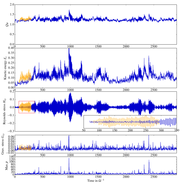
Figure 1: Time-evolution of various quantities, averaged over a box whose size is $L_{x}=20$, $L_{y}=20$ and $L_{z}=3\,H_{0}$. From top to bottom, density-weighted average Toomre parameter $Q$, box average kinetic energy, Reynolds stress, gravitational stress, and density maximum. The resolution is $128\times 128\times 64$ (run PL20-128).

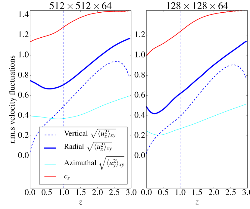
Figure 2: Vertical profiles of turbulent r.m.s velocities, time averaged over $40\,\Omega^{-1}$ for the run PL512 at high resolution (left) and for the run PL128 at low resolution (right)

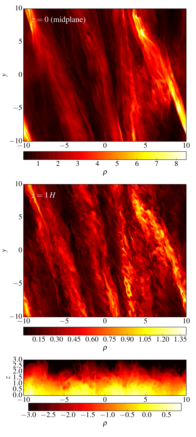
Figure 3: Density snapshots of the 3D gravito-turbulent state obtained in a box of $L_{x}=L_{y}=20H_{0}$ and resolution of $\approx 25$ cells per $H_{0}$ with $\tau_{c}=20\,\Omega^{-1}$. The top panel is a view of the disc midplane $z=0$, the central panel is for $z=H_{0}$, and the bottom panel is a vertical cut, with $\rho$ represented in a logarithmic scale.

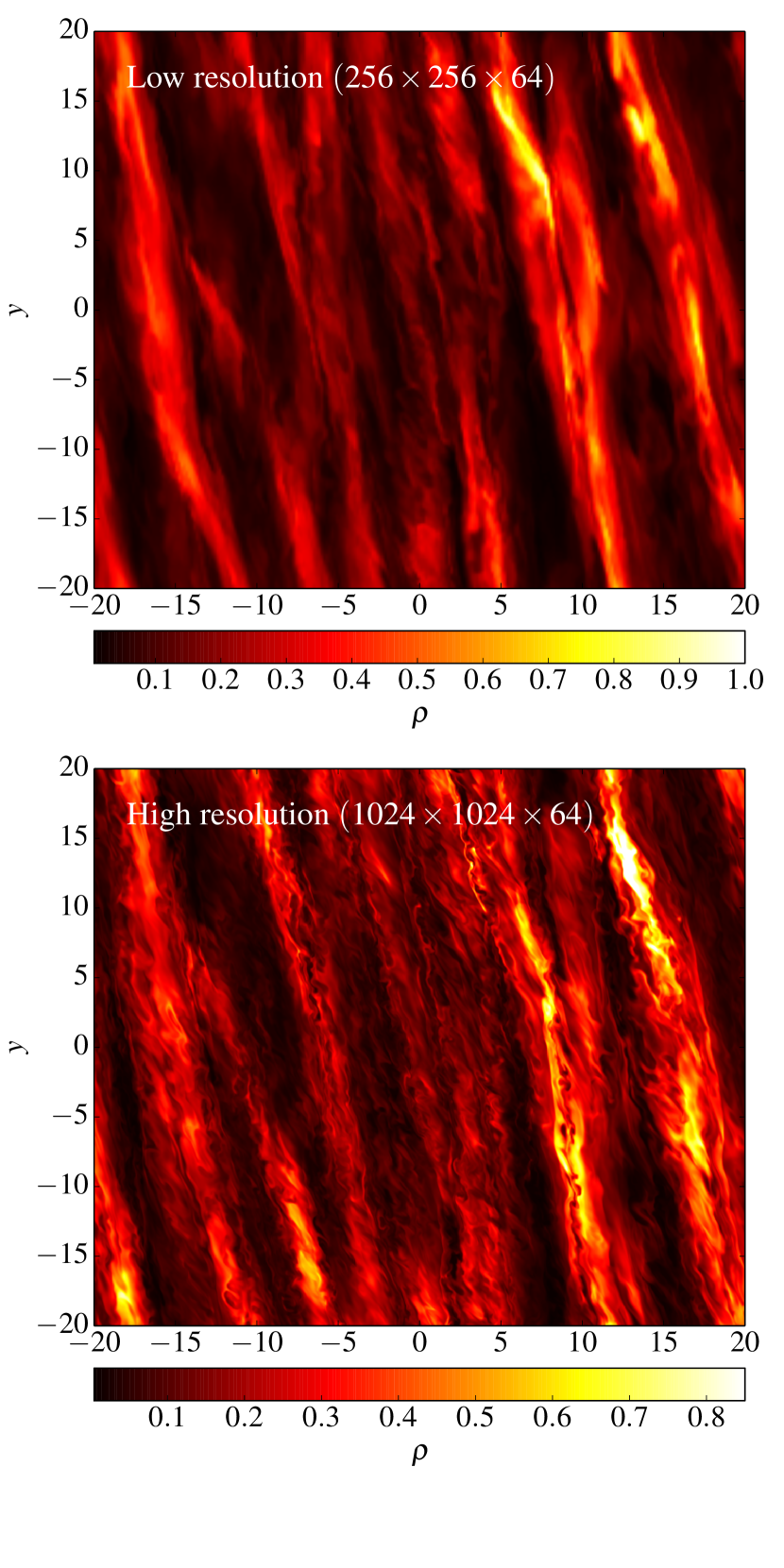
Figure 4: Density snapshots of the 3D gravito-turbulent state obtained in a box of $L_{x}=L_{y}=40\,H_{0}$ at altitude $z=H_{0}$. The top panel comes from a low resolution run of $\approx 6.5$ cells per $H_{0}$ (PL40-256), whereas the bottom panel comes from a high resolution run, $\approx 25$ cells per $H_{0}$ (PL40-1024).

3.2 Dependence on resolution

Next we study how the average turbulent properties depend on grid resolution. For a fixed box size $L_{x}=L_{y}=20\,H_{0}$, we compare four different setups, detailed in Table 1, with 64, 128, 256, 512 points in the horizontal directions (ranging from 3.2 points to $25.6$ points per $H_{0}$.).

Table 1 shows that some quantities like the gravitational stress and Toomre parameter $Q$ do not vary significantly as resolution is increased, provided that $N_{X}\geq 128$. In contrast, the kinetic energy and, in particular, the Reynolds stress differ from one resolution to another, because the higher resolutions simulations have not been run sufficiently long. Recall that in the previous subsection these quantities were shown to vary on periods of thousands $\Omega^{-1}$, but such run times are inaccessible at high resolution (the highest resolved simulations have been run for $\sim 200\,\Omega^{-1}$). The values listed for the kinetic energy and Reynolds stress are probably statistically insignificant.

Run	Resolution	Time (in $\Omega^{-1}$)	$\tau_{c}$	$Q$	$E_{c}$	$U$	$H_{xy}$	$G_{xy}$	$\alpha$
PL20-64	$64\times 64\times 32$	500	20	1.14	0.047	0.332	0.00198	0.00751	0.0176
redPL20-128	$128\times 128\times 64$	3000	20	1.24	0.105	0.396	0.00411	0.00915	0.02005
PL20-256	$256\times 256\times 64$	100	20	1.25	0.115	0.427	0.005	0.0109	0.022
PL20-512	$512\times 512\times 64$	200	20	1.26	0.109	0.412	0.00594	0.00963	0.0226
PL20-128-b	$128\times 128\times 64$	400	20	1.22	0.0762	0.377	0.00376	0.00977	0.0212
PL20-256-RK3	$256\times 256\times 64$	200	20	1.23	0.0741	0.384	0.00509	0.00955	0.0229
PL20-512-$\beta 10$	$512\times 512\times 64$	200	10	1.27	0.126	0.382	0.0091	0.0157	0.039
RO20-128	$128\times 128\times 128$	400	20	1.18	0.0777	0.472	0.00419	0.0112	0.0198
RO20-264	$264\times 264\times 128$	200	20	1.20	0.08	0.489	0.00486	0.0124	0.0212
RO20-264-FL2	$264\times 264\times 128$	200	20	1.19	0.081	0.475	0.00539	0.0118	0.0217
RO20-512	$512\times 512\times 128$	90	20	1.18	0.0754	0.464	0.00488	0.0116	0.0213

Table 1: Parameters and properties of runs in a box of $L_{x}=L_{y}=20H_{0}$. The third columm indicates the time over which quantities have been averaged (not including the transient phase). $Q$ is the average Toomre parameter, $E_{c}$ and $U$ are the box and time-averaged kinetic and internal energy, $H_{xy}$, $G_{xy}$ and $\alpha$ are respectively the averaged Reynolds, gravitational stress and transport efficiency.

Run	Resolution	Time (in $\Omega^{-1}$)	$\tau_{c}$	$Q$	$E_{c}$	$U$	$H_{xy}$	$G_{xy}$	$\alpha$
redPL40-256	$256\times 256\times 64$	100	20	1.38	0.0753	0.4	0.00249	0.0114	0.02115
PL40-512	$512\times 512\times 64$	70	20	1.40	0.132	0.524	0.0034	0.0186	0.025
PL40-1024	$1024\times 1024\times 64$	50	20	1.36	0.076	0.4	0.0028	0.012	0.023
RO40-256	$256\times 256\times 128$	900	20	1.36	0.117	0.625	0.00281	0.0213	0.0233

Table 2: Simulations in larger boxes, $L_{x}=L_{y}=40H_{0}$.

Run	Resolution	Time (in $\Omega^{-1}$)	$\tau_{c}$	$Q$	$E_{c}$	$U$	$H_{xy}$	$G_{xy}$	$\alpha$
redPL80-512	$512\times 512\times 64$	100	20	1.41	0.131	0.523	0.0032	0.0182	0.0244
RO80-512	$512\times 512\times 128$	200	20	1.39	0.149	0.664	1e-6	0.0272	0.0246

Table 3: Simulations in large boxes, $L_{x}=L_{y}=80H_{0}$.

Figure 2 shows the vertical profile of r.m.s velocity fluctuations for PL20-128 and PL20-512 (averaged over $40\Omega^{-1}$). Increasing resolution does not seem to affect the balance between each spatial component, although the radial and azimuthal fluctuations are 1.5 stronger with a resolution of $512$ points in $L_{x}$ and $L_{y}$. We note that vertical motions remain important at $z\geq H_{0}$ whatever the resolution used (even for the lowest one, $N_{X}=64$).

Finally, we visually examined the density snapshots at different altitudes and resolutions. Fig. 3 shows the density structures in the midplane and one scale-height above. At $z=0$, the turbulence is comprised of large scale and distinct spiral waves, of radial lengthscale $\approx 4-5H_{0}$, which break non-linearly. However, at larger $z\simeq H_{0}$ and in higher resolution runs, the coherence of the spiral waves is disturbed by a form of small-scale turbulence. This does not appear in our low resolution runs PL20-128, PL40-256 or PL80-512, nor in previous simulations of 3D gravito-turbulence. Figure 4 shows, in particular, a comparison between different resolutions at $z=H_{0}$ (and for a box of sixe $L_{x}=40\,H_{0}$). Visually these small scale motions take the form of wispy deformations of the spiral wave fronts. These small-scale fluctuations are relatively strong (of order the host density wave), highly non-axisymmetric, and mainly located between $z=0.5\,H_{0}$ and $z=H_{0}$. The density at that location is still relatively high, varying between 0.1 and 1. These small scale features remain visible throughout the simulation and are observed independently of the code, boundary conditions (see section 3.5) and box size (see Fig. 3 and Fig. 4 for comparison).

In conclusion, there is evidence that we achieve convergence for certain mean gravito-turbulent quantities ($Q$ and $G_{xy}$ notably) with resolution, provided that we use more than $5$ grid cells per $H_{0}$ in $x$ and $y$. We cannot decide on the convergence of the kinetic energy $E_{c}$ and Reynolds stress $H_{xy}$, because they exhibit strong fluctuations on times of several hundreds of orbits, of order or longer than our highest resolution simulations. Finally, at resolution larger than $20$ cells per $H_{0}$, we discover a form of small-scale turbulence attacking the large-scale spiral waves. The behaviour of this new dynamical feature with resolution is probably still unconverged. And though its influence on the mean turbulent quantities is probably mild (possibly appearing in the vertical profiles of $u_{x}$ and $u_{y}$), it is readily identified visually in snapshots of the density field, and in later section we show how it can be quantified through various diagnostics.

3.3 Dependence on box size

Another important test, especially for local models, is the box-size dependence of the turbulent properties. Table 1, 2 and 3 show, respectively, a set of simulations computed for $L_{x}=20$, $40$ and $80$ $H_{0}$. To aid comparison, fiducial runs at different box sizes but the same resolution per $H_{0}$ are highlighted in red.

First, doubling the horizontal size from 20 to 40 $H_{0}$ while keeping the resolution per scale height fixed, modifies the average $Q$ only moderately. It is almost 15% larger in PL40-256 compared with PL20-128. This result seems to be robust since it is obtained at different resolutions and with different codes (see Section 3.5). The internal energy also increases. But more strikingly, the ratio between the gravitational and the Reynolds stress is multiplied by a factor 2 or even 3. Unlike the variations of $H_{xy}$ with resolution, this result is statistically robust, since quantities have been recorded for at least 900 $\Omega^{-1}$ (run RO40-256) and the same trend is obtained for all simulations with $L_{x}=40\,H_{0}$. Oscillations of $H_{xy}$ at a frequency of $\Omega$ are still clearly discernible, although their amplitude are weaker and rarely reach negative values.

Finally, for a box even larger, of size $L_{x}=L_{y}=80\,H_{0}$, we show that turbulence properties are comparable to those obtained for $L_{x}=L_{y}=40\,H_{0}$. In particular it appears $Q$ has settled down to a value $\simeq 1.35$-$1.4$. Discrepancies in kinetic energy and Reynolds stress are probably due to insufficient statistics. In conclusion, we have some evidence that there exists some critical $L_{x}=L_{y}$ between 20 and 40 $H_{0}$ above which simulations are converged with respect to the box size. However, further long-term simulations are needed to nail this down.

3.4 Dependence on cooling time

We ran a small number of simulations with different cooling times, not enough to ascertain a critical rate at which fragmentation occurs, but to fix some basic ideas. A high resolution simulation, PL20-512-$\beta$10, using $\tau_{c}=10\,\Omega^{-1}$ and run for $200\,\Omega^{-1}$ shows that $Q$ does not vary significantly compared to when $\tau_{c}=20\,\Omega^{-1}$ (with same resolution). However the average stress is multiplied by a factor 2, as expected from Eq. 18. Note that, despite the shorter cooling time, this simulation failed to exhibit collapsing or even transient fragments. We did check however that when $\tau_{c}=3\,\Omega^{-1}$ the system fragments in less than 20 orbits which supports the results of Shi & Chiang (2014).

3.5 Code comparison and dependence on numerical details

To verify that our results are robust and that the simulated gravito-turbulence does not depend strongly on our numerical implementation, we compare our results with a different code, RODEO. It employs a different Riemann solver, Poisson solver, and boundary conditions (see Sections 2.3.1 and 2.3.2 ).

Tables 1, 2 and 3 show relatively good agreement between the two codes (within the constraints of run-time), in particular for the value of mean $Q$. There are nevertheless some differences: the internal energy is systematically larger in RODEO than in PLUTO. Moreover, in the $L_{x}=80\,H_{0}$ runs, $G_{xy}$ is also larger. These difference remain relatively small and could be due to insufficiently long integrations.

We also checked that simulations run with RODEO depend only mildly on the flux limiter used (see comparison on Table 1 between RO20-264 and RO20-264-FL2). Finally, we show that results are independent of the order of the Runge-Kutta method in the time integrations (see runs PL20-256 and PL20-256-RK3).

4 Small-scale dynamics and axisymmetric oscillations

We showed previously that gravito-turbulent states are characterized by regular oscillations of the Reynolds stress and, in the best resolved simulations, vigorous small-scale dynamics around $z\simeq H_{0}$. In this section, we better understand these structures by extracting their signatures in Fourier space.

4.1 Turbulent power spectra and small-scale structures

We denote by $\widehat{\mathbf{u}}^{w}(k_{x},k_{y},z,t)$ the horizontal 2D Fourier transform of the weighted turbulent velocity field $\rho^{1/3}\mathbf{u}$ (see Section 2.5.2 for definitions). The density-weighted, time-averaged, 2D kinetic energy power spectrum may then be defined through

$$E(k_{x},k_{y},z)=\frac{\Sigma^{1/3}H_{0}^{-1/3}}{2T}\int_{t_{0}}^{t_{0}+T}\left|{\widehat{\mathbf{u}}^{w}(k_{x},k_{y},z,t)}\right|^{2}\,dt,$$ (19)

where the time-average begins at $t=t_{0}$ and is carried out over an interval of duration $T$.

The weighted spectrum, with the one-third scaling in density, is often used in the study of supersonic and compressible turbulence (Lighthill, 1955; Kritsuk et al., 2007). Using simple scaling arguments, one can show that $E(k)\sim k^{-5/3}$ and hence follows the incompressible Kolmogorov power law. Note, however, that this scaling fails for highly compressible forcing and cannot be considered universal (Federrath, 2013).

We define next the time and $k_{x}$-averaged 1D spectrum

$$E_{\text{1D}}(k_{y},z)=\dfrac{1}{k_{x_{0}}}\int E(k_{x},k_{y},z)\,dk_{x},$$ (20)

and the time-averaged isotropic 1D spectrum

$$E_{\text{iso}}(k,z)=\int\int E(k_{x},k_{y},z)\,\delta(|\mathbf{k}^{\prime}|-k)\,dk_{x}dk_{y},$$ (21)

where $|\mathbf{k}^{\prime}|=\sqrt{(k_{x}^{\prime})^{2}+(k_{y}^{\prime})^{2}}$ is the radius in horizontal wavenumber space. The $k_{x}$-averaged spectrum is particularly useful in distinguishing the GI wakes (which possess a low $k_{y}$) from small-scale turbulence (for which $k_{y}$ is bigger). Note that both features may possess comparable $k_{x}$.

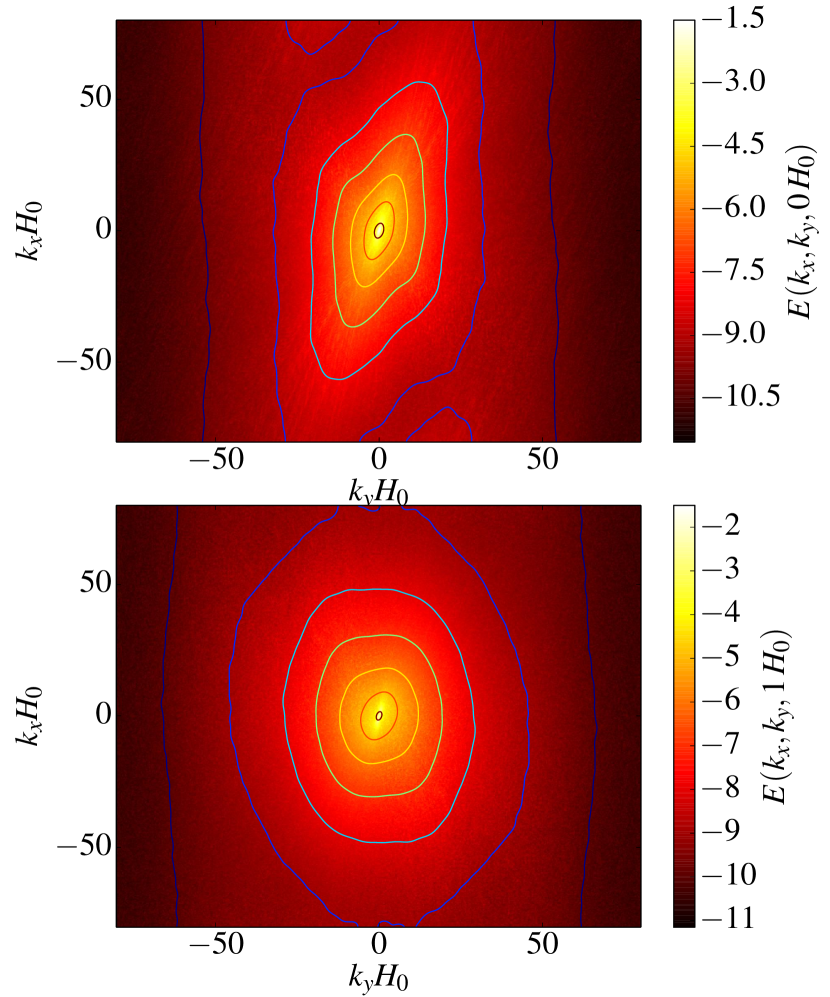
Figure 5: 2D horizontal kinetic energy power spectrum $E(k_{x},k_{y},z)$ as a function of Eulerian wavenumbers in simulation PL20-512. The spectrum is averaged over $40\,\Omega^{-1}$. The top panel is for $z=0$ and the bottom panel is for $z=H_{0}$.

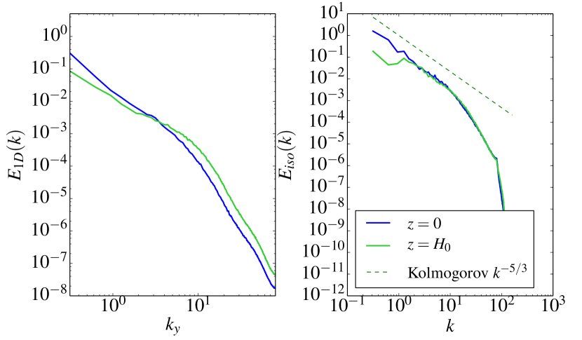
Figure 6: Left: 1D kinetic energy spectrum $E_{\text{1D}}$. Right: 1D isotropic spectrum $E_{\text{iso}}$. Two different altitudes have been considered: blue curves are for $z=0$ and green curve are for $z=H_{0}$. Data are computed from the simulation PL20-512 and averaged in time over $40\Omega^{-1}$.

Figure 5 shows the time-averaged 2D power spectrum of gravito-turbulence $E(k_{x},k_{y},z)$ as a function of the horizontal Eulerian wavenumbers at two different altitudes $z=0$ and $z=H_{0}$. Both spectra are computed from high resolution simulation data (PL20-512) and averaged over $40\,\Omega^{-1}$. For $z=0$, the energy is contained in an inclined elliptical band along the $k_{y}=0$ axis. Turbulent structures are weakly non-axisymmetric and elongated along the azimuthal direction with a small pitch angle. In contrast, at $z=H_{0}$ the signal appears far more isotropic; energy is clearly spread onto small scale non-axisymmetric modes. This broadening of the spectrum is undoubtedly related to the small-scale disturbances afflicting the spiral waves described earlier in Section 3.2.

To better distinguish the small scale motions, we plotted $E_{\text{1D}}(k_{y},z)$, the $k_{x}$-averaged 1D spectrum, in the left panel of Fig. 6 evaluated at $z=0$ and $z=H_{0}$. Note that the ratio of large-scale energy ($k_{y}\leq 2\pi/L_{y}$) to small scale energy ($k_{y}=50$ for instance) strongly varies with altitude $z$. At $z=H_{0}$ this ratio is 15 times smaller than at $z=0$, indicating a significant distribution of energy to smaller scales higher up in the disk. The spectrum in $k_{y}$ appears also less steep for azimuthal scales larger than $0.5H_{0}$, which suggests that the energy of non-axisymmetric modes is injected and cascades differently at those two altitudes. Lower resolution runs do not exhibit nearly the same amount of power on the resolved small-scales at $z=H_{0}$.

Lastly, out of interest we plot the isotropic spectrum $E_{\text{iso}}(k,z)$, even though it is difficult to distinguish the two features in it because both share similar $k_{x}$. Note, however, that the slope of $E(k)$ follows a Kolmogorov law for $k<10H_{0}^{-1}$ but then appears much steeper (well before approaching the grid scale).

In conclusion, the small-scale parasitic turbulence attacking at $z=H_{0}$ is quantifiable and possesses a clear signature in the Fourier decomposition of the flow. This supports the conclusions of the previous section obtained by visual inspection of the density maps. In light of Figs 3, 4 and the present results, we assume that the mechanism producing those small-scale features could be more efficient than a simple inertial turbulent cascade and could be potentially due to a secondary instability of the large scale structure.

4.2 Large scale modes: spiral waves and axisymmetric epicyclic oscillations

The turbulent power spectra shown in Fig. 6 reveals that kinetic energy is not concentrated at wavelengths $\approx 4-5H_{0}$, the typical size of GI density wakes. Apart from the short scales, energy keeps increasing to very large scales $\approx L_{x}$. In this section, we investigate in more detail the nature and origin of these large scale features.

Figure 7 shows the time-evolution of kinetic energy associated with large scale $m=0$ axisymmetric modes (top panel) and $m=1$ non-axisymmetric shearing waves (bottom two panels), in the midplane region $z=0$ and for the run PL20-512. Surprisingly, we found that the largest scale axisymmetric mode ($k_{x}\equiv k_{x_{0}}=2\pi/L_{x},\,\,k_{y}=0$) dominates the energy content. This mode oscillates at a very well-defined angular frequency $\omega_{f}=0.83\,\kappa$, close to the orbital or epicyclic frequency. This is indicative of a large-scale inertial oscillation modified by self-gravity. The mode is clearly responsible for the pseudo-periodic variation of the Reynolds stress observed in Section 3. Smaller scale axisymmetric modes such as $k_{x}=2k_{x_{0}}$ or $k_{x}=3k_{x_{0}}$ are negligible compared to the fundamental mode (their specific energy decreases with their radial scale) and their evolution appears more chaotic.

Figure 7 (bottom panels) shows that, energetically, individual spiral or non-axisymmetric waves grow and decay aperiodically, but their amplitude remains on average weaker than the largest scale axisymmetric mode (in particular $\ell=2$ at $t=42/\Omega$ or the orange and blue ones at $t=57/\Omega$ and $t=60/\Omega$). The energy of the strongly amplified waves evolves quasi-exponentially during their growth phase before soon decaying. Overall the weaker strength of spiral waves is surprising, given that we expect gravito-turbulence to be primarily supported by non-axisymmetric structures (axisymmetric modes being stable for $Q_{\text{turb}}\geq 1$). It is important to note, however, that we only have shown the waves’ kinetic energy. The associated density perturbations associated with spiral waves in fact can be larger than for axisymmetric modes. Indeed, we find that the density of the fundamental axisymmetric mode is rather small and does not oscillate regularly in time.

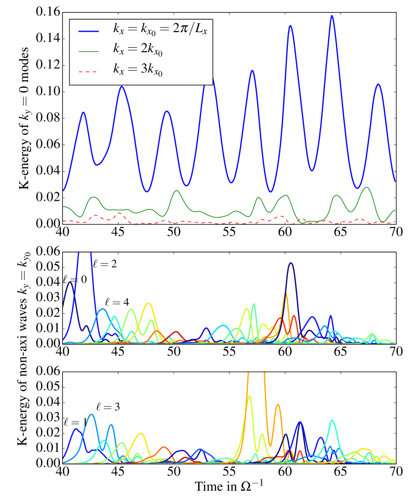
Figure 7: Top: Time-evolution of the kinetic energy $E(k_{x_{0}},0,0)$, $E(2k_{x_{0}},0,0)$ and $E(3k_{x_{0}},0,0)$ associated with the first few axisymmetric modes. Bottom: kinetic energy of several non-axisymmetric shearing waves, with $k_{y}=2\pi/L_{y}$, labelled by their Lagrangian wavenumber $\ell$ (to improve readability, we separate the even $\ell$ in the centre panel from the odd $\ell$ in the bottom panel). All the spectral quantities have been computed in the midplane $z=0$.

Figure 8: Ratio between the kinetic energy of individual axisymmetric modes and the total kinetic energy (averaged over at least $100\,\Omega^{-1}$) as a function of horizontal box size $L_{x}=L_{y}$ (but same resolution per $H_{0}$). Black, purple, blue, green and red account for modes $k_{x}=2\pi/80j$, $j=1,..,5$, in this order. The diamond marker indicates the fundamental mode with wavelength equal to the box size.

Are these axisymmetric modes physical or artificially enhanced by the box size, or even the shearing periodic boundary conditions? To answer this question, we determined the energetics of the axisymmetric structures in larger boxes. Fig. 8 shows that when $L_{x}=40$ and $L_{x}=80\,H_{0}$, the kinetic energy of each individual axisymmetric mode is smaller than when $L_{x}=20\,H_{0}$ but in total represents still $\sim 20\%$ of the energy. Also, for $L_{x}\geq 40\,H_{0}$, the kinetic energy associated with each axisymmetric mode appears to converge to a similar value. Most importantly, for a sufficiently large box, the fundamental mode (on the box size) ceases to be dominant, its place taken by a shorter scale mode. Larger boxes can host multiple axisymmetric inertial oscillations with frequencies close to $\kappa$. These results indicate that the large-scale axisymmetric dynamics is not controlled by the box size, which is consistent with Section 3.2 which showed some turbulent quantities had converged by $L_{x}=L_{y}\gtrsim 40\,H_{0}$.

Finally, we checked that for large boxes, axisymmetric modes still exhibit an oscillatory behaviour with a frequency close to $0.8\kappa$ (this in particular true for the harmonics $k_{x}=2k_{x_{0}}$ or $k_{x}=3k_{x_{0}}$). We checked also that the dynamics and amplitude of these modes are similar in both PLUTO and RODEO simulations. In sum, oscillatory axisymmetric waves are an important component of the GI dynamics, regardless of the box size. Although their amplitude might be enhanced artificially if the box size is too small, their existence is likely to have a physical origin.

4.3 Origin and role of axisymmetric modes

Though non-axisymmetric shearing waves form the backbone of the nonlinear GI dynamics, we have seen that large-scale axisymmetric oscillations are conspicuous participants. Several questions may then be asked:

1. What is their origin? Though linearly stable, how can they reach and sustain large amplitudes?

2. What role do they play in the dynamics? Are they involved in the subcritical transition to, and the maintenance of, turbulence, or are they just passive modes?

In order to answer (a), we determine the force balance associated with the fundamental axisymmetric mode $k_{x}=2\pi/L_{x}$ in PL20-512. It can be decomposed into a high and low amplitude standing wave, $\hat{u}_{1}(t)\cos(k_{x}x)$ and $\hat{u}_{2}(t)\sin(k_{x}x)$ respectively, with $\hat{u}_{1}\gg\hat{u}_{2}$. Figure 9 shows that the first wave possesses an inertial character since it is mainly driven by the Coriolis force and partially restored by pressure. Self-gravity is always opposed to the latter and tends to destabilize the wave (although $Q$ is too large for the wave to become unstable). Nonlinear terms seem negligible in its dynamical evolution, although they have a cumulative positive feedback on its energy budget. We checked that the force balance is similar in the azimuthal direction (not shown here) and for the smaller amplitude second wave. In sum, we identify a coherent quasi-linear epicyclic oscillation. We found that this oscillation is maintained for the entirety of our simulations (which is $3000\,\Omega^{-1}$ for PL20-128b), and the mode cannot be a vestige of our initial condition, since turbulent viscosity would have dissipated it in a shorter timescale (typically $t_{\nu}\simeq 1/(\alpha c_{s}\Omega k^{2})\simeq 500\,\Omega^{-1}$). This suggests that large scale axisymmetric perturbations are nonlinearly excited and regenerated by gravito-turbulence.

We performed several additional simulations, shown in Appendix C, which strongly indicates that the mode $k_{x}=k_{x_{0}}$ is the result of a nonlinear baroclinic interaction between non-axisymmetric density waves. This dynamics is reminiscent of the mode coupling proposed by Laughlin et al. (1997) for gravitoturbulent discs and by Lee (2016) in the context of planet-disc interactions. Laughlin et al. (1997) showed, in particular, that self-interaction of $m=2$ modes can lead to a nonlinear growth of the $m=0$ mode in global discs. However their initial density profile is subject to a Rossby wave instability, which complicates interpretation of their results.

Regarding question (b), there are several reasons to think that these modes are active participants in the disc dynamics. First, they appear to be sufficiently coherent in time to enter in resonance with a pair of inertial waves. Such a resonance, based on a nonlinear triadic interaction, is known to provide a path toward parametric instabilities. We investigate this possibility in the next section.

Second, the large scale axisymmetric modes could be involved in the re-generation and instability of leading shearing waves and thus, in the sustenance of the whole GI dynamics. A potentially related regeneration process has been formulated for the magneto-rotational dynamo problem (Herault et al., 2011). Individual non-axisymmetric wave are sheared out into strongly trailing decaying structure. Long lived dynamics can only be excited if new leading waves are seeded each $\Delta t=\frac{2}{3}L_{y}/L_{x}\Omega^{-1}$. Herault et al. (2011) found that axisymmetric modes play the role of ‘walls’ and thus ‘confine’ the non-axisymmetric waves. The dying trailing structures can then be reflected and give birth to a new leading shearing wave. This mechanism is probably essential to any kind of sustained non-axisymmetric turbulence in the presence of a background shear flow. Analogously, axisymmetric zonal flows are known to support a linear instability of self-gravitating spiral waves (Lithwick, 2007; Vanon & Ogilvie, 2016). We suspect then that such an instability is at work in our simulations of gravito-turbulence and might feature prominently in the self-sustaining process. The dynamics involving the nonlinear regeneration of axisymmetric modes (see previous paragraph and Appendix C) as well as the non-axisymmetric GI linear instability (supported by axisymmetric structures) might form the basis of the fully developed turbulence.

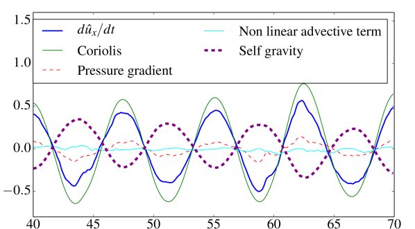
Figure 9: Radial force balance of the large scale axisymmetric mode $k_{x_{0}}=2\pi/L_{x}$ in the midplane region $z=0$.

5 Excitation of a parametric instability

Section 4 revealed that a large-scale axisymmetric epicyclic mode, oscillating at a frequency ${\omega_{F}}\simeq 0.8\,\kappa$, naturally emerges from gravitoturbulence. From the perspective of the smaller scales, this internal coherent oscillation may function equivalently to an external periodic forcing or deformation of the disc. Rotating flows subject to periodic forcing or deformations are known to excite parametric instability (Goodman, 1993); and in fact the standing epicycle we witness in our simulations is similar in many respects to that treated by Fromang & Papaloizou (2007) who showed that an axisymmetric density wave is subject to such an instability. In this section, we explore this idea and consider whether a similar instability occurs in our problem and is responsible for the small scale turbulence appearing at $z\simeq H_{0}$.

5.1 Theoretical expectations

5.1.1 Onset of instability

Parametric instabilities can arise when an oscillator undergoes a forcing at twice its natural frequency. In accretion discs, they occur when a large-scale, time-periodic disturbance enters into resonance with a pair of small-scale inertial waves (Goodman, 1993). This fundamentally 3D instability has been studied exhaustively in the context of eccentric (Ogilvie, 2001; Papaloizou, 2005; Barker & Ogilvie, 2014) and warped discs (Gammie et al., 2000; Ogilvie & Latter, 2013), and in the case of mean-motion resonances between a disc and its companion (Lubow, 1991). More recently, it has been shown to attack spiral density waves excited in the disc (Bae et al., 2016a; Bae et al., 2016b).

Although relatively robust, parametric instabilities require certain conditions to work. If we denote by $\omega_{i_{1}}$ and $\omega_{i_{2}}$ the frequencies of two inertial waves and $\omega_{F}$ the frequency of the large scale oscillation, it is possible to show that growth is obtained when (Fromang & Papaloizou, 2007):

$$\omega_{F}=\omega_{i_{1}}+\omega_{i_{2}}.$$ (22)

To obtain a constraint on the background oscillation $\omega_{F}$, we need the dispersion relation for each inertial wave. This is available in the WKBJ limit of short radial and vertical wavelengths (Goodman 1993). We consider only the coupling of ‘neighbouring’ inertial wave branches, for which $\omega_{i_{1}}\approx\omega_{i_{2}}$, because of the density of the spectrum on short scales. The resonance condition immediately yields

$$\omega_{i_{1}}=\omega_{i_{2}}=\tfrac{1}{2}\omega_{F},$$ (23)

and because $\omega_{i_{1}}^{2}<\kappa^{2}$, we deduce that $\omega_{F}<2\kappa$. From the dispersion relation again, we find that resonance implies $\omega_{i_{1}}^{2}>N^{2}$, and so the condition for the excitation of parametric instability is:

$$2\,N<\omega_{F}<2\,\kappa.$$ (24)

(Goodman, 1993; Fromang & Papaloizou, 2007). As discussed by Bae et al. (2016a), the influence of buoyancy is considerable and must stabilize the flow above a certain disc altitude $z_{\text{crit}}$ for which $N>\kappa$.

We should emphasize that these simple theoretical arguments have their limits. First, condition (24) is derived for axisymmetric disturbances, though for weakly non-axisymmetric waves $(k_{y}\ll k)$ Goodman (1993) showed that condition (24) still holds. Unlike axisymmetric waves, however, their lifetime is finite and they can only be amplified transiently. Second, condition (24) only applies to localised wave packets, and not to vertically global modes. In principle one could solve the full linear eigenvalue problem with vertical structure, similarly to Ogilvie & Latter (2013) and Barker & Ogilvie (2014), but we leave this task for another time. In any case, given the disordered background in which the inertial waves find themselves, they may manifest more as localised packets rather than larger-scale organised structures. Finally, self-gravity has been neglected, though for $Q\simeq 1$ and $k_{x}$ large, the dispersion relation of linear inertial disturbance is almost unchanged when compared to the case without self-gravity (see Fig. 3 in Mamatsashvili & Rice (2010)).

In the isothermal case, Fromang & Papaloizou (2007) estimated the growth rate of parametric instability due to an axisymmetric density wave to be roughly proportional to the product of the fractional amplitude of the density wave and $\omega_{F}$. Applying this formula to the large-scale epicyclic oscillations in our simulations this gives a growth rate $\sim 0.1-0.2\,\Omega$, and so we expect the parametric instability to develop after few orbits in our simulations, unless it is impeded by other participants in the gravitoturbulence.

5.1.2 Propagation and breaking of inertial waves

Suppose that the conditions for exciting inertial waves are met. How do these waves propagate and dissipate in the disc? First note that, as a localised wave packet travels upwards from the midplane, the background state around it changes and, as a consequence, the wave packet properties will also change. In fact, the wave will ‘refract’ and become ‘channeled’ by the disk’s vertical structure, which acts similarly to a wave-guide (Lubow & Pringle, 1993; Bate et al., 2002). The packet’s upward trajectory will bend more and more radially, before ultimately settling into a normal eigenmode of the vertically global problem, travelling solely in the radial direction.

Perhaps before that occurs, the wave will break nonlinearly. In an unstratified medium, inertial waves are known to break down into turbulence via the action of secondary instabilities, driven by shear, which occurs when displacements are comparable to wavelengths. If the inertial wave has a form $\hat{u}\exp{\text{i}(k_{\xi}\xi-\omega t)}$ where $\xi$ is in the direction of propagation, then breaking occurs when the particle velocities exceed the phase velocity

$$\hat{u}\approx\omega/k_{\xi}.$$ (25)

This relation is equivalent to saying the Rayleigh stability criterion is locally violated (the angular momentum gradient becomes locally negative, see Wienker (2016)). This secondary instability is actually then another parametric instability involving a primary inertial wave and two daughter waves. The route to turbulence in such systems may then be viewed as a cascade of parametric instabilities.

In a stratified disc, inertial waves naturally break as they propagate toward the surface of the disc. Indeed, since the density decreases above the midplane, the velocity components increase with $z$ (consider the linear eigenfunctions of a stratified disk, Appendix A). We expect inertial waves to break above a critical height that depends on the mode structure. For instance, a $n=1$ inertial mode, for which $\hat{u}_{x}\propto z$ (see Appendix A), possesses a critical height around $z\simeq H_{0}$. Higher order $n$ modes break at altitudes somewhat lower, but all are consistent with our observation of small-scale activity above the midplane. Most of the kinetic energy transfers to small scale at this critical height or above. Energy is then expected to saturate at a value of order $u^{2}=\omega^{2}/k_{\xi}$, although a more complete calculation, in the context of eccentric discs, shows that it also increases with the amplitude of the parent wave Wienker (2016).

5.2 Evidence of parametric instability from the numerical data

5.2.1 Temporal spectra

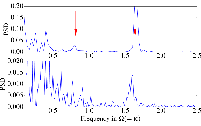
Figure 10: Power spectral density (PSD) of the averaged kinetic energy as a function of temporal frequencies. The upper panel was obtained from simulations PL20-512 and the lower panel from PL20-128. The red arrows on the right indicate the frequency of the axisymmetric oscillation (note that the kinetic energy oscillates at twice the natural frequency of the mode). The left arrows show a secondary peak at 0.8 $\kappa$, which might correspond to the resonant inertial modes.

In Section 4 we identified a large scale axisymmetric mode that oscillates at a frequency $\omega_{F}\approx 0.8\kappa$. According to condition (24), a parametric instability is then possible in the vicinity of the midplane where $N=0$ and should induce the growth of a pair of inertial waves at a frequency $\omega=\omega_{F}/2$. To assess whether or not the instability occurs in our simulations, we compute the temporal Fourier spectrum of the turbulent signal. Fig 10 (top) shows the power spectrum of the box-averaged kinetic energy as a function of (temporal) frequencies for the PL20-512 run. A strong peak is observed at a frequency $2\omega_{F}$, which corresponds to the large-scale axisymmetric mode (quadratic quantities like energy oscillate at twice the frequency of the associated mode). From the right to the left, we see a second peak, smaller in amplitude, at half the frequency of the fundamental peak $\omega=\omega_{F}$. If we look further to the left, several distinct peaks are seen respectively at $\omega=\omega_{F}/2$ and $\omega=\omega_{F}/4$. This cascade of subharmonics peaks at frequency $\omega_{F}/2^{n}$ may be interpreted as a direct signature of parametric instability via inertial mode couplings.

A similar result is obtained from the PSD of PL20-128, calculated over a much longer time $3000\,\Omega^{-1}$, although the signal is more noisy and the peaks less pronounced. Because of the rich assortment of long-time variability (discussed in Section 3.1) it is difficult to extract as clear a signature of the parasitic inertial waves, as in the shorter time high-resolution run PL20-512.

In a larger boxes with $L_{x}=40\,\Omega^{-1}$ and $L_{x}=80\,\Omega^{-1}$, the signal is spread over more frequencies and the spectrum is more difficult to interpret. Now multiple large-scale axisymmetric modes are hosted in the box with similar frequencies (cf. Fig. 8), each potentially unstable to different parametric resonances. The ensuing turbulent dynamics is more complicated and the temporal spectrum a less useful diagnostic in this case.

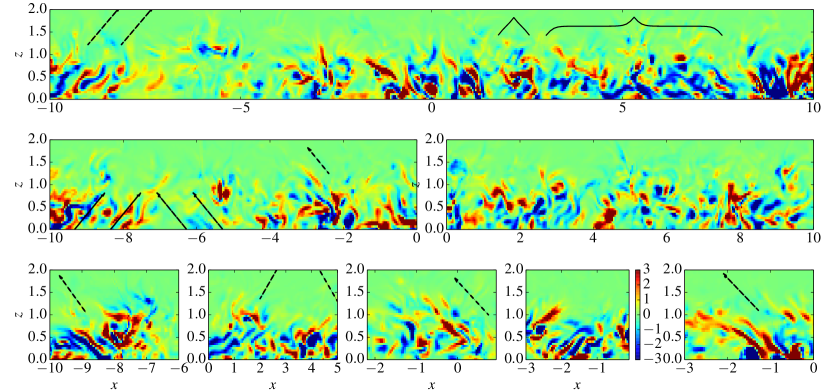
Figure 11: Helicity in the poloidal $(x,z)$ plane weighted by the average density profile in $z$, for different time. All arrows indicate a direction of $45\degree$ with respect to the vertical axis. The curly brackets shows some examples of intricate and tangled patterns probably associated with inertial waves. In any of these figures, it is possible to see an alternation of inclined red and blue bands, with typical wavelength $\approx 0.1-0.2H_{0}$

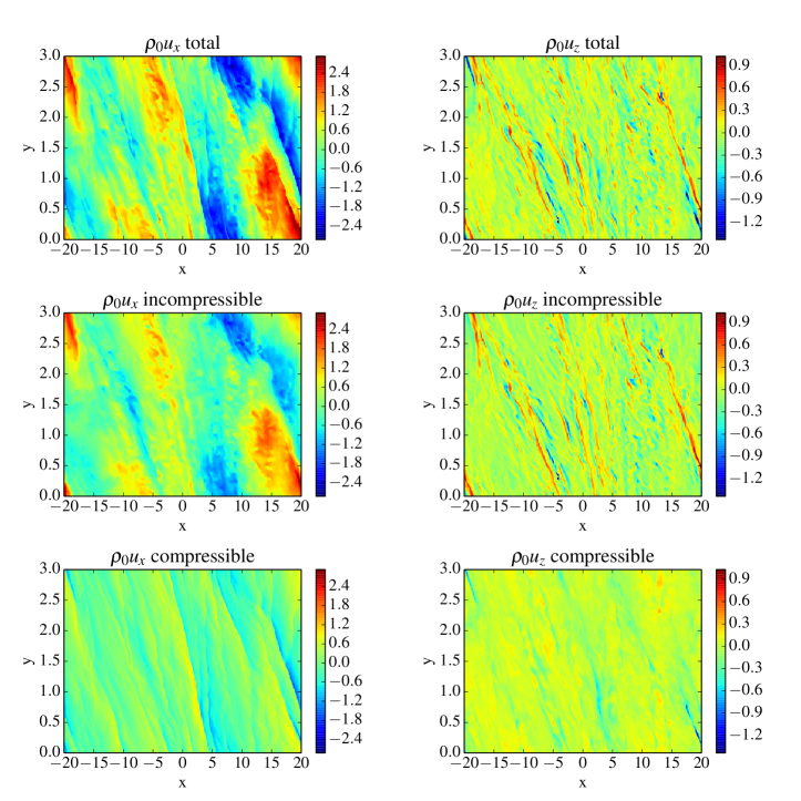
Figure 12: Velocity components $u_{x}$ (left) and $u_{z}$ (right) in the mid plane $z=0$, weighted by the average density at that location. The top panels represent the total field, the center and bottom panels represent respectively its incompressible and compressible parts.

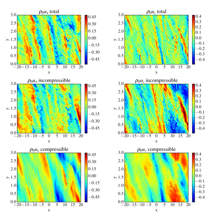
Figure 13: Velocity components $u_{x}$ (left) and $u_{z}$ (right) in the plane $z=H_{0}$, weighted by the average density at that location. The top panels represent the total field, the center and bottom panels represent respectively its incompressible and compressible parts.

5.2.2 Helicity maps

Another way to trace the inertial waves and the associated parametric instability is to compute the helicity of the flow

$$\mathcal{H}=\mathbf{u}\cdot(\mathbf{\nabla}\times\mathbf{u}).$$ (26)

Because inertial waves satisfy $\mathbf{\nabla}\times\mathbf{u}\simeq\pm k\mathbf{u}$, where $k$ is their wavenumber, they are intrinsically helical. The direction of propagation of a given packet corresponds to a surface of constant helicity. These different properties have been studied in particular in the context of the solar and geodynamo (Ranjan & Davidson, 2014; Davidson, 2014; Wei, 2015; Singer & Olson, 1984).

Figure 11 shows the helicity $\mathcal{H}$, weighted by the averaged vertical density profile, projected onto the $(x,z)$ plane at different $y$ and times. Helical structures have a typical size of $\lesssim H$, in both the $z$ and $x$ directions. They form inclined and interleaved layers of positive and negative helicity, corresponding to the troughs and crests of inertial waves. Thus the associated wavevectors cut across the layers, while the group velocities point along the layers (Bordes et al. 2012). In Fig. 11 the inclined black arrows have been superimposed to highlight the inertial layers.

The preferential angle of propagation is in a range between $\pm 30\degree$ and $\pm 50\degree$ measured from the vertical axis. However, using the local, linear and axisymmetric dispersion for inertial waves (Goodman, 1993), and setting $\omega_{i}=\frac{1}{2}\Omega_{F}\approx 0.42\kappa$, we find that unstable inertial waves should possess a group velocity pointing within a range of angles $\lesssim 30\degree$ with respect to the rotation axis. The slight discrepancy with the simulation data we attribute to wave channelling by the disk structure, as discussed earlier. In fact, the bottom right panel of Fig. 11 presents a nice example of wave channeling.

5.2.3 Helmholtz decomposition and connection with the small-scale turbulence

We showed in Sections 3.2 and 4.1 vigorous small-scale turbulent activity taking place $z\sim H_{0}$, while in the previous subsection we compiled numerical evidence for inertial waves propagating upward at altitudes less than $H_{0}$. In this subsection we attempt to connect the two.

First we check that the small-scale motions are not directly excited by large-$k$ gravitational modes. We performed a simulation, starting from a gravito-turbulent state, taken from PL20-512, and filtered the gravitational potential on small-scales by retaining only modes with $k_{x}<6k_{x_{0}}$ and $k_{y}<6k_{y_{0}}$. Despite the filtering, the small-scale turbulence persisted for long times in the reconfigured simulation.

This activity, however, might still consist of a field of small-scale p-modes, different in character to inertial waves. In fact, short wavelength linear p-modes preferentially localise at the disk surface (Korycansky & Pringle, 1995; Ogilvie, 1998), where the turbulence is observed. They may be generated by disordered motions on large-scales, in particular by the nonlinearly breaking of large-scale wakes, which may favour the less-dense upper layers.

One way to disentangle these different small-scale motions is to decompose the velocity field into compressible and incompressible parts. Inertial waves are generally incompressible (or rather anelastic) if they vary on a vertical scale comparable or less than the background support ($\bar{k}_{z}\lesssim 1$). On the other hand, p-modes are associated with compressible motions, though they are not necessarily curl-free and can also possess an incompressible part. To separate the compressible part of a vector field $\mathbf{F}$ from its incompressible part, we use the Helmholtz decomposition:

$$\mathbf{F}=\mathbf{F}_{\text{c}}+\mathbf{F}_{\text{ic}}=\mathbf{\nabla}\varphi+\mathbf{\nabla}\times\mathbf{{\Phi}},$$ (27)

where $\varphi$ is a scalar field, defined up to a constant and $\mathbf{\Phi}$ a vector field defined up to a gradient field. The first term is the compressible and potential part of $\mathbf{F}$. This is a curl free component, i.e $\mathbf{\nabla}\times\mathbf{F}_{\text{c}}=0$. The second term is the incompressible and solenoidal part, and it is divergence free, i.e $\mathbf{\nabla}\cdot\mathbf{F}_{\text{ic}}=0$. Applying the divergence operator on both sides of Eq. (27) and using the solenoidal properties, we obtain

$$\nabla^{2}\varphi=\mathbf{\nabla}\cdot\mathbf{F}.$$ (28)

Therefore, to find the potential $\varphi$, we have to solve a Poisson equation with a source term $\mathbf{\nabla}\cdot\mathbf{F}$. In the shearing box frame, the method is very similar to the one used to obtain the disk’s potential (see Section 2.3.2), so we simply adapted our Poisson solver to deal with a different source term. Several tests on simple flows were completed before applying our method to the full turbulent field. The calculation of $\mathbf{\Phi}$ requires solving three Poisson equations but in practice we obtain it by substracting the compressible part from the initial field $\mathbf{F}$.

We applied the Helmholtz decomposition to the vector $\mathbf{F}=\rho_{0}\,\mathbf{u}$, where $\rho_{0}$ is the vertical profile of the horizontally-averaged density. This decomposition permits us to analyse the incompressibility of the flow, remembering that the incompressible component $(\rho_{0}\,\mathbf{u})_{ic}=\mathbf{\nabla}\times\mathbf{{\Phi}}$ will preferentially exhibit an inertial character.

Figure 12 shows the incompressible (centre panels) and compressible parts (bottom panels) of the flow components $\rho_{0}\,u_{x}$ and $\rho_{0}\,u_{z}$ in the midplane $z=0$. For the radial component $\rho_{0}\,u_{x}$, the two parts have similar amplitudes and both exhibit large-scale spiral waves. In the incompressible part the waves manifest as large-scale features, while in the compressible part they are visible as thin shocks. In addition, we observe small-scales bundles, of typical size 0.2 $H_{0}$, in the incompressible part exclusively. The vertical velocity (right panels) is clearly dominated by the incompressible component, which exhibits thin filament structures organised along the wakes. We attribute both the small vertical velocity filaments and the horizontal bundles with incompressible inertial waves developing at the midplane.

Figure 13 shows the same decomposition at $z=H_{0}$. Here the small-scale dynamics is far more developed, in both the radial and vertical velocities. Most importantly, however, is that these small-scale features are almost completely confined to the incompressible parts of both velocity components. The compressible parts exhibit predominantly large-scale structure associated with the gravity wakes, in the case of $u_{z}$ arising probably from the vertical breathing or splashing of the wakes. There is no evidence of small-scale p-modes as might be generated by wave breaking at this altitude. In summary, the marked incompressibility of small-scale turbulence at $z=H_{0}$ is strong evidence that it is indeed comprised of inertial waves excited by parametric instability, breaking and mixing at these altitudes (as described in Section 5.1.2).

6 Conclusions and astrophysical implications

We performed a set of 3D vertically stratified shearing-box simulations of gravitoturbulence, reproducing the local behaviour of marginally gravitationally unstable discs. For a fixed cooling time $\tau_{c}=20\,\Omega^{-1}$, we provided evidence showing that averaged turbulent properties converge for box size larger than $40\,H_{0}$ and for sufficient resolution. The convergence of some quantities, however, are difficult to ascertain, such as the kinetic energy and Reynolds stress, due to their bursty and very long time variation (hundreds of orbits).

Our highest resolution runs exhibit small-scale disordered motions at around $z\approx H_{0}$. It is unclear whether the properties of this small-scale turbulence have yet converged. We compile theoretical and numerical evidence that the origin of the turbulence is a parametric instability involving a pair of inertial waves and a large-scale axisymmetric epicycle emerging naturally from the gravitoturbulence. It is likely that this large-scale mode is an important participant in the onset and sustenance of nonlinear non-axisymmetric GI.

We discount alternative causes of the turbulence. Kelvin-Helmholtz instability arising from the gravity wakes’ horizontal shearing should lead to activity at all altitudes, not just at $z=H_{0}$. Nonlinear breaking of the gravity wakes should lead to compressible motions, but we show that the small-scale turbulence is primarily incompressible at $z=H_{0}$. Finally, vertical splashing due to wake collisions should give rise to larger-scale motions dominated by the vertical velocities, which is numerically observed only in the compressible part of the flow. The small-scale turbulence we find is incompressible and not dominated by vertical motions.

It should be stated clearly that our simulations employ large horizontal domains ($>20H$) for which it is challenging to justify the locality of the shearing box model. This is certainly the case for the thicker PP disks, where $H/r\sim 0.05$, but there is more lee-way with AGN. We persist with this numerical tool because it affords us a well-defined and relatively clean platform to probe shorter-scale dynamics at high resolution. Previous grid-based global simulations can compete on vertical resolution, but suffer from poor azimuthal resolution especially (e.g. Michael et al., 2012; Steiman-Cameron et al., 2013). The radial boundary conditions in global simulations impose further complications that muddy their interpretation.

There are several astrophysical implications of this work. We focus on those most relevant to PP disks. Small-scale turbulence disturbs the coherence of the large-scale spiral waves, while not exactly destroying them. This ‘scrambling’ may be possible to observe in direct imaging of large-scale spiral arms, giving them a somewhat ‘flocculent’ appearance (see discussion in Bae et al., 2016b).

Perhaps of greatest importance is the impact of small-scale turbulence on marginally coupled particles off the midplane. Two-dimensional planar simulations of GI and dust indicate that this class of particle can collect in filaments, sometimes achieving overdensities two orders of magnitude over the background. Moreover, their relative velocities are diminished to below 1% of the sound speed, facilitating gravitational collapse (Gibbons et al., 2012, 2014, 2015; Shi et al., 2016). If, however, within these filaments there is an additional source of turbulent motions, on a similar scale (as we find), then such overdensities may be difficult to attain, and gravitational collapse more difficult. Moreover, because the eddy-sizes of the parasitic turbulence are $\ll H$ it is more likely that pre-collisional pairs are decorrelated and will thus have large impact speeds. However, for these effects to be significant the vertical thickness of the particle subdisk must be $\lesssim H$, and this may not always be a situation that lasts very long in the coupled evolution of the disk and dust.

More generally, small-scale turbulence will enhance whatever diffusion is present. Figure 2 shows that better resolved turbulence exhibit larger rms velocities by factors $\sim 1$, and one would expect diffusivities to be similarly enhanced. As mentioned earlier, even our highest resolved simulations are still probably unconverged with respect to this physics.

Though not explored in this paper, small-scale motions may make fragmentation more difficult. It should be emphasised that the typical inertial wave motions may be too slow to be effective, and being localised to $z\sim H$ will certainly be inefficient at the midplane where most fragmentation begins. Work specifically targeting fragmentation in high resolution 3D disk models will appear in a separate paper.

Finally, one may ask how these features affect the magnetohydrodynamics in PP and AGN disks, as both may be moderately well-ionised in their outer regions (Menou & Quataert, 2001; Turner et al., 2014). The preponderance of helical motions automatically provide a means of dynamo action, but the magnetorotational instability (in some non-ideal form) must also play a role here. One may then imagine a rich and complex interplay between the GI, the parasitic turbulence feeding off it, and the magnetorotational instability.

Appendix A Background equilibrium

We present in this appendix several tests to verify that our self-gravity module in PLUTO and boundary conditions are correctly implemented in 3D. Note that the 2D linear problem (both axisymmetric and non-axisymmetric) has been already checked in Riols & Latter (2016). In the presence of self-gravity the vertical background equilibrium is governed by Eqs. (7) and (8), where $c_{s_{0}}$ and $\rho_{0}$ denote the sound speed and the density in the midplane. By introducing the ‘isothermal’ Toomre parameter

$$Q_{{2D}_{0}}=\dfrac{c_{s_{0}}\Omega}{\pi G\Sigma},$$

and the dimensionless $\bar{z}=z/H_{0}$, $\bar{\rho}=\rho/\rho_{0}$ as well as the ratio $\Delta=4H_{0}\rho_{0}/\Sigma$, the set of equation (7)-(8) reduce to a single dimensionless equation:

$$\dfrac{1}{\gamma}\dfrac{d}{d\bar{z}}\left[\dfrac{1}{\bar{\rho}}\dfrac{d\bar{\rho}^{\gamma}}{d\bar{z}}\right]+1+\dfrac{\Delta}{Q_{{2D}_{0}}}\bar{\rho}=0.$$ (29)

We numerically solve this equation by use of a finite difference method. We impose $\Sigma=1$ and a certain value for $Q_{{2D}_{0}}$. Imposing these two quantities makes the calculation somewhat tricky because the midplane density $\rho_{0}$, and hence $\Delta$, are not known in advance. It is then necessary to begin with a guess for $\rho_{0}$ and to refine the solution iteratively, using a shooting method, until the surface density matches our prescription.

Note that the isothermal Toomre parameter defined here is not exactly equal to the $Q$ in the simulations, as the density-weighted average $c_{s}$ differs from the midplane one. However the sound speed profile associated with the equilibrium scales as $\rho^{1/3}$ with $\gamma=5/3$, so that the difference between $Q_{{2D}_{0}}$ and $Q$ defined in Section 2.5 is small.

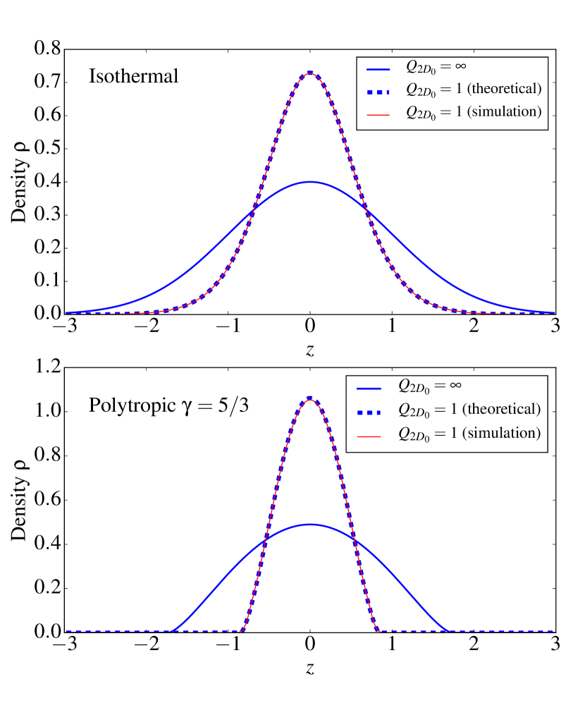
Figure 14: Density profiles of disc equilibria, for an isothermal gas (top) and polytrope with $\gamma=5/3$ (bottom) (fixed $\Sigma=1$). The solid blue line corresponds to the theoretical profile computed from Equation (29) without self-gravity ($Q_{{2D}_{0}}=\infty$) while the dashed thick blue line is computed for $Q_{{2D}_{0}}=1$. In each cases, the thin red line is the density profile obtained with PLUTO after $100\,\Omega^{-1}$ and is almost indiscernible from the theoretical one.

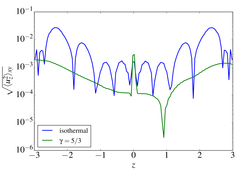
Figure 15: Vertical profile of the r.m.s vertical velocity fluctuations at $t=100\Omega^{-1}$ excited by vertical boundary conditions.

Figure 14 shows different density (and pressure) profiles for an isothermal gas ($\gamma=1$) and a polytropic gas with $\gamma=5/3$, obtained by numerical integration of Eq. 29. When self-gravity is included and $Q$ is of order 1, the disc becomes more compressed and its effective height, defined such that $\rho=e^{-0.5}\rho_{0}$, is $H_{\text{eff}}=0.52H_{0}$ for the isothermal case and $H_{\text{eff}}=0.41H_{0}$ for the polytrope.

For $Q_{{2D}_{0}}=1$, we use these semi-analytical density profiles (and the associated pressure) as an initial condition in PLUTO. We ran the code for $100\,\Omega^{-1}$ and checked that the density has not evolved during that time (see the red solid lines in Fig. 14). We also plot in Fig. 15 the vertical profile of velocity fluctuations at $t=100\,\Omega^{-1}$. For stable configurations, the fluctuation amplitude remains smaller than $10^{-2}c_{s_{0}}$. For a polytrope, these fluctuations can be larger than the local sound speed, but do not influence the equilibrium in the midplane. This shows that the boundary conditions are correctly implemented and do not introduce too much noise, even for the extreme case of a polytrope for which the density is floored to a certain value in the upper atmosphere.

Appendix B Linear axisymmetric modes

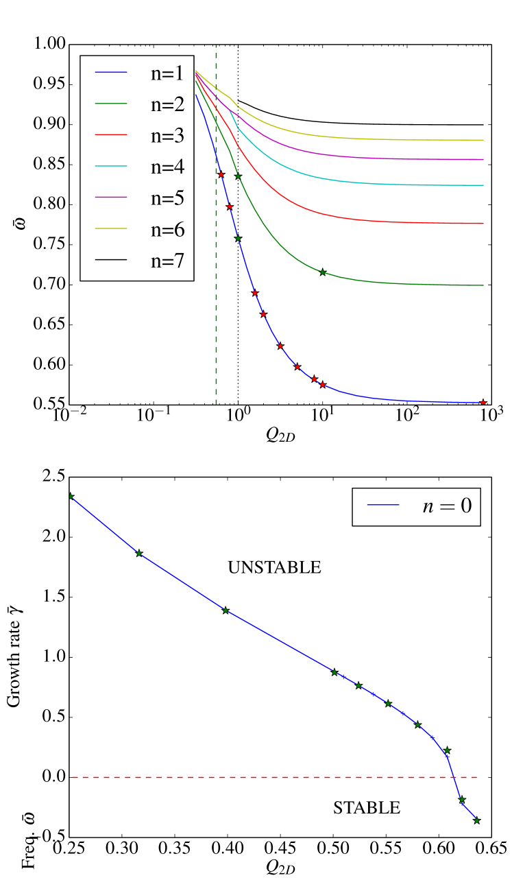
Figure 16: Properties of linear axisymmetric modes in the local isothermal thin disc approximation. Top panel: dependence of the wave frequency $\omega$ on $Q_{{2D}_{0}}$ for the inertial branch modes $n=1,2,...,7$. Bottom panel: growth rates of the first unstable $n=0$ mode. In all cases $\bar{k}_{x}=2\pi/5$. Solid curves are theoretical growth rates or frequencies, calculated with the linear eigensolver. Red and green stars are the values obtained from PLUTO simulations, with resolution of 256 and 512 points per azimuthal wavelength, respectively. The dotted line is $Q_{2D}=1$ while the dashed line represents the critical $Q_{2D}$ for which the $n=0$ mode becomes unstable.

To further test our Poisson solver in PLUTO, we simulate the linear solutions and compare them with semi-analytic calculations. Unlike the 2D case, it is not possible to analytically derive a dispersion relation and we need to solve numerically the full eigenvalue problem. We restrict our analysis to the isothermal case and assume axisymmetric density and velocity perturbations of the form $\left[\hat{\rho}(z),\,\hat{\mathbf{u}}(z)\right]\,\exp(\text{i}k_{x}x-\text{i}\omega t)$. We denote by ${\rho}={\rho}_{e}(z)$ and $\Phi_{e}(z)$ the density and potential equilibrium, respectively. We normalize densities (background and perturbations) by the midplane density $\rho_{0}$, velocities by the uniform sound speed $c_{s_{0}}$, and pressure by $\rho c_{s_{0}}^{2}$. Finally by introducing the dimensionless wave frequency $\bar{\omega}=\omega/\Omega$ and wavelength $\bar{k}_{x}=k_{x}H_{0}$, the linearized and normalized system of equations reads

$$-\text{i}\bar{\omega}\hat{\rho}+\text{i}\bar{k}_{x}\rho_{e}\hat{u}_{x}+\dfrac{d}{d\bar{z}}(\rho_{e}\hat{u}_{z})=0$$ (30)

$$\rho_{e}(-\text{i}\bar{\omega}\hat{u}_{x}-2\hat{u}_{y})=-\text{i}\bar{k}_{x}\hat{P}-\text{i}\bar{k}_{x}\rho_{e}\hat{\Phi}$$ (31)

$$\rho_{e}(-\text{i}\bar{\omega}\hat{u}_{y}+\dfrac{1}{2}\hat{u}_{x})=0$$ (32)

$$\rho_{e}(-\text{i}\bar{\omega}\hat{u}_{z})=-\dfrac{d\hat{P}}{d\bar{z}}-\hat{\rho}\left(\bar{z}+\dfrac{d\Phi_{e}}{d\bar{z}}\right)-\rho_{e}\dfrac{d\hat{\Phi}}{d\bar{z}}$$ (33)

$$\left(\dfrac{d^{2}}{d\bar{z}^{2}}-\bar{k}_{x}^{2}\right)\hat{\Phi}=\dfrac{\hat{\rho}\Delta}{Q_{2D_{0}}}$$ (34)

Solutions to this problem without self-gravity have been produced by Lubow & Pringle (1993) for an isothermal stratified disc and by Korycansky & Pringle (1995) and Ogilvie (1998) in the case of a polytropic disc. More recently the self-gravitating problem was tackled by Mamatsashvili & Rice (2010).

The eigenfunctions in an isothermal non-self-gravitating disk are the Hermite polynomials and the dispersion relation is

$$(-\bar{\omega}^{2}+n)(-\bar{\omega}^{2}+1)-\bar{k}_{x}^{2}\bar{\omega}^{2}=0$$ (35)

where $n$ is the order of the Hermite polynomial and is related to the vertical structure of the mode (the number of nodes in the eigenfunctions). There exists two branches of solutions for each $n>0$, a low frequency branch with $\bar{\omega}<1$ which has an inertial character and a high frequency branch with $\bar{\omega}>1$ which has an acoustic character. Note that the case $n=0$ is often considered separately. At frequencies larger than the epicyclic, it corresponds to a two-dimensional acoustic-inertial wave, which can be associated with an f-mode (free surface oscillation) for the polytropic case.

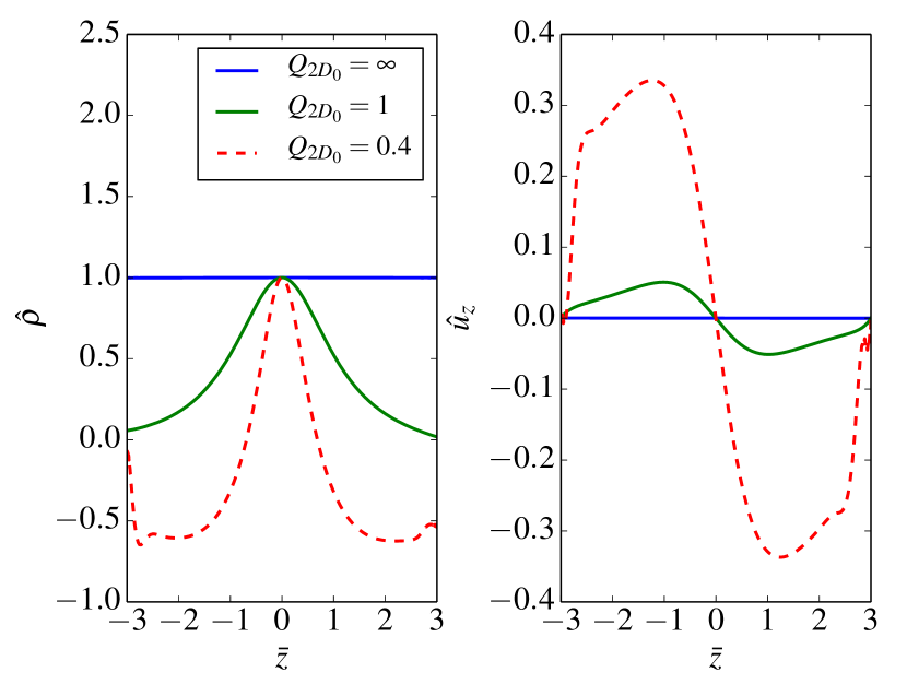
Figure 17: Vertical structure of the $n=0$ eigenmode for 3 different $Q_{{2D}_{0}}=\{\infty,\,\,1,\,\,0.4\}$. Left to right: density and vertical velocity perturbations. Note that the mode is normalized such that $\hat{\rho}(z=0)=1$. The noise at the boundary (in particular for $Q_{{2D}_{0}}=0.4$) results from the fact that we are solving the linear problem for the momentum and not for the velocity components directly.

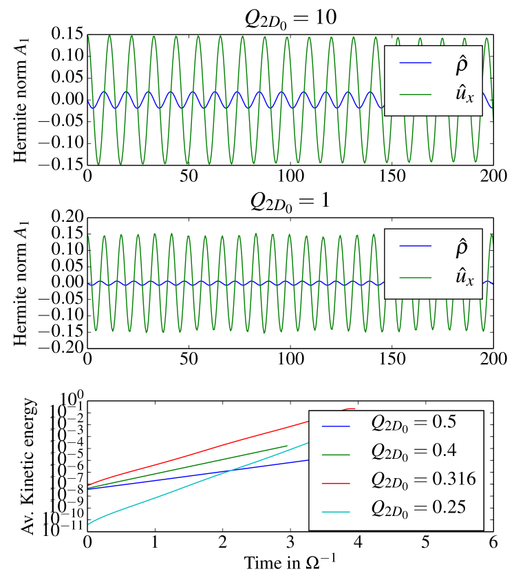
Figure 18: The top two panels describe the time evolution of the density and radial velocity perturbation of the $n=1$ inertial mode for different values of $Q_{{2D}_{0}}$ (amplitudes of perturbations are expressed in terms of the Hermite norm, defined through Eq. (36)) The last panel shows the evolution of the average kinetic energy for the $n=0$ mode for four values of $Q_{{2D}_{0}}$.

We restrict our study to the isothermal case and a fixed $\bar{k}_{x}=2\pi/5$. The surface density is set to $\Sigma=1$. For a given value of the Toomre parameter $Q_{{2D}_{0}}$, we first compute the corresponding background density and gravitational potential, using the methods described in Appendix A (the equilibria fixes the value of $\Delta$, which depends on $Q_{{2D}_{0}}$). We then compute the eigenvalues $\bar{\omega}_{i}$ and corresponding eigenmodes of the linearized system, using a Chebyshev collocation method on a Gauss-Lobatto grid. This method results in a matrix eigenvalue problem that can be solved using a QZ method (Golub & Van Loan, 1996; Boyd, 2001). Numerical convergence is guaranteed by comparing eigenvalues for different grid resolutions and eliminating the spurious ones. The vertical domain has a size $6H_{0}$ and is resolved by a maximum resolution of 600 points. Boundary conditions for perturbed modes are $\rho_{e}\mathbf{\hat{u}}=0$ (momentum tends to 0) and $d\hat{\Phi}/d\hat{z}=\pm\hat{k_{x}}\hat{\Phi}$ (justified if the background density decreases quasi-exponentially).

When self-gravity is negligible, $Q_{{2D}_{0}}=\infty$, we checked that the eigenvalues match the dispersion relation (35) and that for $n>0$ there exist two different types of solutions corresponding to either $\bar{\omega}>1$ (p modes) or $\bar{\omega}<1$ (r modes). We then vary $Q_{{2D}_{0}}$ and focus first on the modes with inertial character. For each branch labelled $n=1,2,...,7$, ($n$ defined as the order of the Hermite polynomial in the limit $Q_{{2D}_{0}}=\infty$), we plot in the top panel of Fig. 16 the evolution of the wave frequency as a function of $Q_{{2D}_{0}}$. We find that $\bar{\omega}$ decreases with increasing $Q_{{2D}_{0}}$ but never becomes complex (unstable), at least for the range of $Q_{{2D}_{0}}$ studied ($0.25<Q_{{2D}_{0}}<\infty$). Instead, the gravitational unstable mode is associated with the inertial-acoustic branch $n=0$ (f modes). The corresponding eigenfunction has no structure in $z$ for $Q_{{2D}_{0}}=\infty$ but appears to develop some structure as $Q_{{2D}_{0}}$ is decreased. Figure 17 shows in particular that the vertical velocity component of the unstable mode develops an odd symmetry as for $n=1$.

Having solved the linear problem directly, we check that our version of PLUTO reproduces its main results in simulations of stable and unstable axisymmetric waves. For that purpose, we used a box of size $5H\times 5H\times 6H$ (full disc in $z$) and introduced at $t=0$ a perturbation with $k_{x}=2\pi/L_{x}$, $k_{y}=0$ whose vertical shape is determined by the eigensolver (in addition to the background density equilibrium). Figure 18 shows the density and radial velocity amplitude of the $n=1$ inertial mode, expressed in terms of the Fourier-Hermite norm

$$A_{n}(X)=\int\int\hat{X}(z)\cos(k_{x}x)H_{e_{n}}(z)\mathrm{e}^{-z^{2}/2}d_{x}d_{z}$$ (36)

for $Q_{{2D}_{0}}=1$ and $10$. At a resolution of $256\times 1\times 256$, the solution remains periodic and conserves its vertical shape for more than $200\,\Omega^{-1}$. The wave frequencies, inferred from these plots, are superimposed on the dispersion diagram of Fig. 16 and compared with the theoretical frequencies, for different $Q_{{2D}_{0}}$ (red stars denoted a resolution of $256\times 1\times 256$ whereas green stars is for a resolution of $512\times 1\times 512$). We find a very good agreement between the frequencies computed with the eigensolver and those measured from the simulations. The relative error remains always smaller than 1% (typically the mean error is 0.3%). We have undertaken a similar test for the $n=2$ branch, although only 2 points have been computed in that case.

Finally we simulated the $n=0$ branch which becomes unstable for $Q_{{2D}_{0}}=0.63$. Fig 18 (bottom) shows the evolution of the averaged kinetic energy in the box for different $Q_{{2D}_{0}}$. Growth rates are easily measured by computing the slope of these curves. In Fig 16 (bottom panel), we superimpose the numerical growth rate obtained (green stars) with the predicted growth rate as a function of $Q_{{2D}_{0}}$. We found again that numerical and theoretical growth rate match remarkably well, even for small values of $Q_{{2D}_{0}}$.

Appendix C Nonlinear ‘instability’ of axisymmetric modes

Figure 19: Top: Time evolution of the specific kinetic energy in the midplane $z=0$ of the fundamental axisymmetric mode $k_{x}=k_{x_{0}}$ in the box $L_{x}=40H_{0}$. Bottom: energy budget of the fundamental axisymmetric perturbation. Each curve represents the cumulative work associated with a term (or a force) in the Navier-Stockes equation.

Simulations of gravito-turbulence in shear flows exhibit strong large scale axisymmetric motions (see Section 4). To better understand how these motions are generated by the turbulent flow, we perform a simple experiment: we considered a gravito-turbulent state in a small box $L_{x}=20H_{0}$ and we used the symmetry of the shearing box to construct a stacked version of this state in a box of twice the original size. We then examined the midplane time-evolution of the fundamental axisymmetric mode $k_{x}=k_{x_{0}}$, which possesses a wavelength the size of the new box. The results are summarized in Fig. 19. At $t=0$, the energy associated with this mode is zero, since we started from a state computed in box of half size. The mode is forced by non-linearities and grows with a typical growth rate $\gamma_{a}=0.3\Omega$. Its short term evolution is very stochastic, but its long-term evolution is more or less exponential.

To understand the nature of this instability, we investigated the kinetic energy budget of this fundamental mode:

$$\dfrac{1}{2}\dfrac{d\mathbf{u_{F}}^{2}}{dt}=\frac{3}{2}u_{x_{F}}u_{y_{F}}+\mathbf{u_{F}}\cdot\nabla\mathbf{\Phi}-\mathbf{u_{F}}\cdot\left(\dfrac{\nabla P}{\rho}\right)_{F}-\mathbf{u_{F}}\cdot(\mathbf{u}\cdot\nabla\mathbf{u})_{F}$$ (37)

The subscript ‘F’ denotes here the fundamental axisymmetric mode $k_{x}=k_{x_{0}}$ or its related projection for nonlinear terms . On the right hand side, the two first linear terms are associated with the background shear and self-gravity. The third and fourth terms are related to the pressure gradient and nonlinear advection. The pressure gradient term can be decomposed into a linear and nonlinear part:

$$\left(\dfrac{\nabla P}{\rho}\right)_{F}=\left(\dfrac{\nabla P}{\rho}\right)^{NL}_{F}+\left(\dfrac{\nabla{P}_{F}}{\rho_{0}}\right)$$ (38)

where $\rho_{0}$ is the midplane background density.

Figure 19 (bottom) shows the cumulative contribution of each term involved in the mode growth. First, we found that the work done by self-gravity is mainly negative and hence does not participate in the instability. This is expected since the axisymmetric mode is gravitationally linearly stable. The shear term $-Su_{x_{0}}u_{y_{0}}$ is also stabilizing. Note that the Coriolis force does no work since it only redistributes energy from the $y$ component to the $x$ component or vice-versa.

The main contribution to the kinetic energy, at least for the first orbits, is clearly the nonlinear term associated with the pressure work. Physically, this term corresponds to a baroclinic effect, due to the misalignement of pressure and density gradients. Indeed, if the pressure term is assumed to be dominant in the energy evolution of the axisymmetric mode, then the vorticity equation reduces to:

$$\dfrac{\partial\bm{\omega}}{\partial t}=\dfrac{\bm{\nabla}P\times\bm{\nabla}\rho}{\rho^{2}}.$$ (39)

The formation of axisymmetric cells associated with vorticity aligned in the $y$ direction is possible if baroclinic non-axisymmetric perturbations (or spiral waves) interact with each other. In other words, if the average in $y$ of $({\bm{\nabla}P\times\bm{\nabla}\rho})_{F}\cdot\bm{\hat{y}}$ has a positive feedback.

A possible origin for the global process is a triadic interaction between the $m=1$ spiral density waves and axisymmetric modes. The scenario can be described as follows: non-axisymmetric waves tap into two reservoirs of energy which are the shear and the self-gravity. The nonlinear interaction between a swinging leading wave and a dying trailing wave produces an axisymmetric modulation (through the baroclinic term), which in turn reinforces the non-axisymmetric waves, via a mechanism similar to that described in Lithwick (2007). This scenario provides a potential explanation for why axisymmetric modes are growing exponentially, despite the absence of a classical ‘linear’ instability.

References

- Bae et al. (2016a) Bae J., Nelson R. P., Hartmann L., Richard S., 2016a, ApJ, 829, 13
- Bae et al. (2016b) Bae J., Nelson R. P., Hartmann L., 2016b, ApJ, 833, 126
- Balbus & Papaloizou (1999) Balbus S. A., Papaloizou J. C. B., 1999, ApJ, 521, 650
- Barker & Ogilvie (2014) Barker A. J., Ogilvie G. I., 2014, MNRAS, 445, 2637
- Bate et al. (2002) Bate M. R., Ogilvie G. I., Lubow S. H., Pringle J. E., 2002, MNRAS, 332, 575
- Boss (1997) Boss A. P., 1997, Science, 276, 1836
- Boyd (2001) Boyd J. P., 2001, Courier Dover
- Cameron (1978) Cameron A. G. W., 1978, Moon and Planets, 18, 5
- Christiaens et al. (2014) Christiaens V., Casassus S., Perez S., van der Plas G., Ménard F., 2014, ApJl, 785, L12
- Davidson (2014) Davidson P. A., 2014, Geophysical Journal International, 198, 1832
- Durisen et al. (2007) Durisen R. H., Boss A. P., Mayer L., Nelson A. F., Quinn T., Rice W. K. M., 2007, Protostars and Planets V, pp 607–622
- Federrath (2013) Federrath C., 2013, MNRAS, 436, 1245
- Fromang & Papaloizou (2007) Fromang S., Papaloizou J., 2007, AA, 468, 1
- Fukagawa et al. (2013) Fukagawa M., et al., 2013, PASJ, 65, L14
- Gammie (2001) Gammie C. F., 2001, ApJ, 553, 174
- Gammie et al. (2000) Gammie C. F., Goodman J., Ogilvie G. I., 2000, MNRAS, 318, 1005
- Gibbons et al. (2012) Gibbons P. G., Rice W. K. M., Mamatsashvili G. R., 2012, MNRAS, 426, 1444
- Gibbons et al. (2014) Gibbons P. G., Mamatsashvili G. R., Rice W. K. M., 2014, MNRAS, 442, 361
- Gibbons et al. (2015) Gibbons P. G., Mamatsashvili G. R., Rice W. K. M., 2015, MNRAS, 453, 4232
- Goldreich & Lynden-Bell (1965) Goldreich P., Lynden-Bell D., 1965, MNRAS, 130, 125
- Golub & Van Loan (1996) Golub G., Van Loan C., 1996, Matrix Computations. Johns Hopkins Studies in the Mathematical Sciences, Johns Hopkins University Press, https://books.google.fr/books?id=mlOa7wPX6OYC
- Goodman (1993) Goodman J., 1993, ApJ, 406, 596
- Goodman (2003) Goodman J., 2003, MNRAS, 339, 937
- Herault et al. (2011) Herault J., Rincon F., Cossu C., Lesur G., Ogilvie G. I., Longaretti P.-Y., 2011, Phys. Rev. E, 84, 036321
- Hirose & Shi (2017) Hirose S., Shi J.-M., 2017, MNRAS, 469, 561
- Kalas et al. (2008) Kalas P., et al., 2008, Science, 322, 1345
- Korycansky & Pringle (1995) Korycansky D. G., Pringle J. E., 1995, MNRAS, 272, 618
- Koyama & Ostriker (2009) Koyama H., Ostriker E. C., 2009, ApJ, 693, 1316
- Kritsuk et al. (2007) Kritsuk A. G., Padoan P., Wagner R., Norman M. L., 2007, in Shaikh D., Zank G. P., eds, American Institute of Physics Conference Series Vol. 932, Turbulence and Nonlinear Processes in Astrophysical Plasmas. pp 393–399 (arXiv:0706.0739), doi:10.1063/1.2778991
- Laughlin et al. (1997) Laughlin G., Korchagin V., Adams F. C., 1997, ApJ, 477, 410
- LeVeque (2002) LeVeque R., 2002, Finite Volume Methods for Hyperbolic Problems. Cambridge Texts in Applied Mathematics, Cambridge University Press, https://books.google.co.uk/books?id=QazcnD7GUoUC
- Lee (2016) Lee W.-K., 2016, ApJ, 832, 166
- Lighthill (1955) Lighthill M., 1955, 2
- Lithwick (2007) Lithwick Y., 2007, ApJ, 670, 789
- Lubow (1991) Lubow S. H., 1991, ApJ, 381, 259
- Lubow & Pringle (1993) Lubow S. H., Pringle J. E., 1993, ApJ, 409, 360
- Mamatsashvili & Rice (2010) Mamatsashvili G. R., Rice W. K. M., 2010, MNRASs, 406, 2050
- Menou & Quataert (2001) Menou K., Quataert E., 2001, ApJ, 552, 204
- Michael et al. (2012) Michael S., Steiman-Cameron T. Y., Durisen R. H., Boley A. C., 2012, ApJ, 746, 98
- Mignone et al. (2007) Mignone A., Bodo G., Massaglia S., Matsakos T., Tesileanu O., Zanni C., Ferrari A., 2007, ApJs, 170, 228
- Ogilvie (1998) Ogilvie G. I., 1998, MNRAS, 297, 291
- Ogilvie (2001) Ogilvie G. I., 2001, MNRAS, 325, 231
- Ogilvie & Latter (2013) Ogilvie G. I., Latter H. N., 2013, MNRAS, 433, 2403
- Paardekooper (2012) Paardekooper S.-J., 2012, MNRAS, 421, 3286
- Papaloizou (2005) Papaloizou J. C. B., 2005, AAp, 432, 743
- Ranjan & Davidson (2014) Ranjan A., Davidson P. A., 2014, Journal of Fluid Mechanics, 756, 488
- Rice et al. (2014) Rice W. K. M., Paardekooper S.-J., Forgan D. H., Armitage P. J., 2014, MNRAS, 438, 1593
- Riols & Latter (2016) Riols A., Latter H., 2016, MNRAS, 460, 2223
- Roe (1981) Roe P. L., 1981, Journal of Computational Physics, 43, 357
- Roe (1986) Roe P. L., 1986, Annual Review of Fluid Mechanics, 18, 337
- Shi & Chiang (2014) Shi J.-M., Chiang E., 2014, ApJ, 789, 34
- Shi et al. (2016) Shi J.-M., Zhu Z., Stone J. M., Chiang E., 2016, MNRAS, 459, 982
- Shlosman & Begelman (1987) Shlosman I., Begelman M. C., 1987, Nature, 329, 810
- Singer & Olson (1984) Singer H. A., Olson P. L., 1984, Geophysical Journal, 78, 371
- Steiman-Cameron et al. (2013) Steiman-Cameron T. Y., Durisen R. H., Boley A. C., Michael S., McConnell C. R., 2013, ApJ, 768, 192
- Toomre (1964) Toomre A., 1964, ApJ, 139, 1217
- Turner et al. (2014) Turner N. J., Lee M. H., Sano T., 2014, ApJ, 783, 14
- Vanon & Ogilvie (2016) Vanon R., Ogilvie G. I., 2016, MNRAS, 463, 3725
- Wallin et al. (1998) Wallin B. K., Watson W. D., Wyld H. W., 1998, ApJ, 495, 774
- Wei (2015) Wei X., 2015, Geophysical and Astrophysical Fluid Dynamics, 109, 159
- Wienker (2016) Wienker A., 2016, Master of Philosophy