A Hybrid Approach with Multi-channel I-Vectors and Convolutional Neural Networks for Acoustic Scene Classification

Abstract

In Acoustic Scene Classification (ASC) two major approaches have been followed . While one utilizes engineered features such as mel-frequency-cepstral-coefficients (MFCCs), the other uses learned features that are the outcome of an optimization algorithm. I-vectors are the result of a modeling technique that usually takes engineered features as input. It has been shown that standard MFCCs extracted from monaural audio signals lead to i-vectors that exhibit poor performance, especially on indoor acoustic scenes. At the same time, Convolutional Neural Networks (CNNs) are well known for their ability to learn features by optimizing their filters. They have been applied on ASC and have shown promising results. In this paper, we first propose a novel multi-channel i-vector extraction scheme for ASC, improving their performance on indoor and outdoor scenes. Second, we propose a CNN architecture that achieves promising ASC results. Further, we show that i-vectors and CNNs capture complementary information from acoustic scenes. Finally, we propose a hybrid system for ASC using multi-channel i-vectors and CNNs by utilizing a score fusion technique. Using our method, we participated in the ASC task of the DCASE-2016 challenge. Our hybrid approach achieved $1^{\text{st}}$ rank among 49 submissions, substantially improving the previous state of the art.

I Introduction

The field of Computational Auditory Scene Analysis (CASA) is a fast moving area, with international challenges such as DCASE  to accelerate the progress on complex audio recognition problems. Previously, methods based on feature engineering from speech and music domain such as MFCCs, Linear Predictive Coefficients and Gammatone Cepstral Coefficients[1] have been used to extract features for ASC.

More sophisticated techniques have been developed to overcome the complexities caused by the noise and other unwanted acoustic phenomena. Such methods manipulate the engineered feature spaces to create a better acoustic representation to distinguish between different acoustic scenes. For example, i-vector features[2] use MFCCs to create a low-dimensional latent space for short audio segments.

In contrast with feature engineering techniques, there exist methods that learn an internal representation from spectograms or similar representations of audio by optimizing their parameters. Examples of such methods are Non-negative Matrix Factorization (NMF) [3] and CNNs [4].

In the scientific society there are many discussions about the use of feature engineering approaches versus feature learning methods. The authors of this paper believe that CASA could benefit from the best of both worlds. Therefore, we introduce a hybrid approach for ASC. The aim of this work is threefold:

1. We introduce a novel multi-channel i-vector extraction scheme for ASC using tuned MFCC features extracted from both channels of audio.

2. Using a CNN architecture inspired by VGG style networks we show that we can achieve comparable performances to the state of the art in ASC. Also, we show that i-vectors and CNNs provide complementary information from the acoustic scenes.

3. Finally, we demonstrate an efficient way of fusing i-vectors with CNNs. We propose a hybrid ASC system using multi-channel i-vectors, CNNs, and a score-fusion technique.

II I-vector Features

The i-vector [2] representation has been used in different areas such as speech [5, 6], music classification [7] and ASC [8]. I-vectors are segment-level representations computed from acoustic features (e.g., MFCCs) of audio segments. They provide a fixed-length and low-dimensional representation for audio excerpts containing rich acoustic information. In short, i-vectors are latent variables representing the shift of an audio segment from a universal distribution, usually referred to as Universal Background Model (UBM).

The UBM is trained on the acoustic features of a sufficient amount of audio segment examples to capture the distribution of the acoustic feature space. To extract the i-vector of an audio segment, the UBM model is first adapted to acoustic features of the segment and the parameters of the adapted model are considered as a new representation for the audio segment.

Second, to capture the shift of the adapted model from the UBM a Factor Analysis (FA) procedure is applied. The parameters of the adapted model are decomposed into a factor with lower dimensioality and better discrimination power. The i-vector itself, is a maximum a postriori (MAP) estimation of this low-dimensional factor.

The UBM is usually a Gaussian Mixture Model (GMM) trained on MFCCs. To apply the FA, the adapted GMM mean supervector $\mathbf{M_{s}}$ – which is adapted to an audio segment from the scene $s$ – can be decomposed as follows:

$$\mathbf{M_{s}}=m+\mathbf{T}.y_{s}$$ (1)

where $m$ is the UBM mean supervector and $\mathbf{T}.y_{s}$ is an offset that captures the shift from the UBM. The low-dimensional vector $y_{s}$ is a latent variable with a normal prior and its respective i-vector is a MAP estimate of $y_{s}$. The factorization matrix $\mathbf{T}$ is learned via expectation maximization.

II-A The I-vector pipeline

To use the i-vector features for ASC, we apply a series of processing blocks known as i-vector pipeline. Our i-vector pipeline consists of 3 phases: 1) development, 2) training and 3) testing. During the development phase, the UBM is trained and the adapted models for each audio segment in the development set are computed. Then using these adapted models, the $\mathbf{T}$ matrix is trained.

In the training phase, i-vectors of the training set are extracted by utilizing the i-vector models (UBM and $\mathbf{T}$) and the length of i-vectors are normalized to one [10]. Using these training set i-vectors, a Linear Discriminant Analysis (LDA) [11] and a Within-Class Covariance Normalization (WCCN) [12] model is trained. The LDA and WCCN projection matrices are used for projecting i-vectors in order to reduce the within-class variability and maximize the class separation in the i-vector space. Afterwards, the class-averaged i-vectors are stored as the model i-vector for each class.

In the testing phase, the i-vectors are extracted, length-normalized and projected by using the previously trained models (UBM, $\mathbf{T}$, LDA, WCCN). Each resulting i-vector from the test set is then compared to all the model i-vectors by applying cosine scoring [13]. Finally, the class represented by its model i-vector with the highest score, determines the predicted class.

Our UBM is trained with 256 Gaussian components on MFCC features extracted from audio excerpts. The UBM, $\mathbf{T}$ matrix, LDA and WCCN projections are trained on the training portion of each Cross Validation (CV) split. The dimensionality of the i-vector space is set to 400. The configuration of MFCC features are discussed in the following section.

III Multi-channel I-Vector Extraction Scheme

To improve the performance of i-vectors for ASC, we propose a novel multi-channel i-vector extraction scheme. Our scheme can be explained in 3 steps: 1) MFCC parameter tuning, 2) multi-channel i-vector extraction and 3) score averaging. We first demonstrate a parametrization of MFCC features, tuned for i-vector extraction for ASC. Further, we explain how we use the multi-channel signals for i-vector extraction. Finally, we describe the score averaging technique.

III-A Boosting MFCCs for i-vector extraction

In [14] it was shown that it is useful to find a good parametrisation of MFCCs for a given task. Therefore, the first step is to improve the performance of MFCCs which we extract with the Voicebox toolbox[15]. The results in this section are always averaged from a four-fold CV.

To investigate different observation window lengths, we place the different observation windows symmetrically around the frame that was always fixed on 20 ms. Thus, independent of the actual observation window, we always end up with exactly the same amount of observations. In Table I we provide the results of different windowing schemes for MFCCs and their deltas and double deltas. As can be seen, the impact of using different overlaps is quite severe on the results of the MFCCs. Experimental results suggest that a 20 ms window without overlap gives best accuracy using i-vectors extracted from MFCCs. The effect is much smaller on the results of deltas and double deltas. Nevertheless, we consider it useful to extract deltas and double deltas separately with a 60 ms observation window, and combine them with the 20 ms MFCCs into one single feature vector.

(%)	window length			coefficients
	win=20 ms	win=60 ms	win=100 ms	w/ $0^{th}$	w/o $0^{th}$
$MFCC$	68.95	61.84	60.61	68.95	71.43
$\Delta$	61.62	64.02	60.68	61.62	56.34
$\Delta\Delta$	61.54	62.05	59.49	61.54	50.77

TABLE I: Results of MFCC tuning. Gray cells indicate the configurations that were combined for further experiments.

After fixing observation window lengths for MFCCs and deltas and double deltas, we evaluate the amount of coefficients that is actually useful in our specific setting. Often, the $0^{th}$ coefficient is ignored in order to achieve loudness invariance, which is also helpful for ASC. The results in Table I support this intuition, where we can see that including the $0^{th}$ coefficient leads to reduced accuracy for i-vectors extracted from MFCCs. Nevertheless, including the delta and double delta of the $0^{th}$ MFCC is in the feature vectors shows performance improvement as shown in Table I.

The configuration used to extract MFCC boosted i-vectors are as follows. We use 23 MFCCs (without $0^{th}$ MFCC) extracted by applying a 20 ms observation window without any overlap. 18 MFCC deltas (including the $0^{th}$ MFCC delta), and 20 MFCC double deltas (including the $0^{th}$ MFCC double delta) are extracted by applying a 60 ms observation window, placed symmetrically around a 20 ms frame. Regardless of the observation window length, we use 30 triangle shaped mel-scaled filters in the range [0-11 kHz].

III-B Multi-channel Feature Extraction

Most often, the binaural audio material is down-mixed into a single monaural representation by simply averaging both channels. This could be problematic in cases where an important cue is only captured well in one of the channels, since averaging would then lower the SNR, and increase the chance that it gets missed by the system. The analysis of both channels separately would alleviate this problem.

Not only do we extract MFCCs from both channels separately, but also from the averaged monaural representation as well as from the difference of both channels. All in all, we extract MFCCs from four different audio sources, resulting in four different feature space representations per audio file. An experiment where we concatenated the MFCCs into a single feature vector did not lead to improved i-vector representations, therefore we opt for a score-averaging approach.

(%)	fold 1	fold 2	fold 3	fold 4	avg
BAS	78.97	64.48	68.46	77.5	72.24
Single-ch.	84.14	68.28	75.17	75.00	75.65
Multi-ch.	85.86	76.55	77.52	83.22	80.79

TABLE II: Comparing the performance of the i-vector system that uses our tuned MFCCs, with the provided MFCCs. BASE: original MFCC provided by the DCASE organisers; Single-channel: tuned MFCCs on averaged single-channel; multi-channel: multi-channel tuned MFCCs.

The aforementioned separately extracted MFCCs yield four different i-vectors and LDA-WCCN models which in turn result in four different cosine scores per audio file. In order to fuse those scores, we simply compute the mean of them and use it as the final score for each audio excerpt.

IV Deep Convolutional Neural Networks

As mentioned in the introduction, one of the contributions of this work is to study the differences between approaches using feature engineering and feature learning in ASC. In this section, we describe the neural network architecture as well as the optimization strategies used for feature learning in our ASC network.

The specific network architecture used is depicted in Table III. The feature learning part of our model follows the VGG style networks for object recognition and the classification part of the network is designed as a global average pooling layer as in the Network in Network architecture[16]. The input size of our network is a one channel spectrogram excerpt with size $149\times 149$. This means we train the model not on whole sequences but only on small ”sliding” windows. The spectrograms for this approach are computed as follows: The audio is sampled at a rate of $22050$ samples per second. We compute the Short Time Fourier Transform (STFT) on $2048$ sample windows at a frame rate of $31.25$ FPS. Finally we post-process the STFT with a logarithmic filterbank with 24 bands, logarithmic magnitudes and an allowed passband of $20$Hz to $16$kHz. The parameters of our models are optimized with mini-batch stochastic gradient decent and momentum. The mini-batch size is set to $100$ samples. We start training with an initial learning rate of $0.02$ and half it every 5 epochs. The momentum is fixed at $0.9$ throughout the entire training. In addition we apply an $L2$-weight decay penalty of $0.0001$ on all trainable parameters of our model.

For classification of unseen samples at test time we proceed as follows. First we run a sliding window over the entire test sequences and collect the individual class probabilities for each of the window. In a second step we average the probabilities of all contributions and assign the class with maximum average probability.

Input $1\times 149\times 149$
$5\times 5$ Conv(pad-2, stride-2)-$32$-BN-ReLu
$3\times 3$ Conv(pad-1, stride-1)-$32$-BN-ReLu
$2\times 2$ Max-Pooling + Drop-Out($0.3$)
$3\times 3$ Conv(pad-1, stride-1)-$64$-BN-ReLu
$3\times 3$ Conv(pad-1, stride-1)-$64$-BN-ReLu
$2\times 2$ Max-Pooling + Drop-Out($0.3$)
$3\times 3$ Conv(pad-1, stride-1)-$128$-BN-ReLu
$3\times 3$ Conv(pad-1, stride-1)-$128$-BN-ReLu
$3\times 3$ Conv(pad-1, stride-1)-$128$-BN-ReLu
$3\times 3$ Conv(pad-1, stride-1)-$128$-BN-ReLu
$2\times 2$ Max-Pooling + Drop-Out($0.3$)
$3\times 3$ Conv(pad-0, stride-1)-$512$-BN-ReLu
Drop-Out($0.5$)
$1\times 1$ Conv(pad-0, stride-1)-$512$-BN-ReLu
Drop-Out($0.5$)
$1\times 1$ Conv(pad-0, stride-1)-$15$-BN-ReLu
Global-Average-Pooling
$15$-way Soft-Max

TABLE III: Model Specifications. BN: Batch Normalization, ReLu: Rectified Linear Activation Function, CCE: Categorical Cross Entropy. For training a constant batch size of 100 samples is used.

V Score Fusion

To fuse the multi-channel i-vector cosine scores with the soft-max activation probabilities of our VGG-net, a score fusion technique is carried out. We use a Linear Logistic Regression (LLR) model to learn the fusion parameters. Our LLR learns the coefficients $\alpha_{k}$ and bias $\beta$ to fuse the likelihoods of $K$ different models by maximizing $C^{\prime}_{llr}$ where:

$$\begin{split}{\vec{l^{\prime}}(x_{n})}=\sum\limits_{k=1}^{K}\alpha_{k}\cdot\vec{l_{k}}(x_{n})+\beta\\ C^{\prime}_{llr}=-\frac{1}{N}\sum\limits_{n=1}^{N}w_{c}\log P^{\prime}_{n}\end{split}$$ (2)

and $C$ is the number of our classes and $N$ is the total number of our likelihood examples. $\vec{l_{k}}(x_{n})$ is the $n^{\text{th}}$ likelihood from the model $k$, $P^{\prime}_{n}$ is the posterior probability for the true class of $n^{\text{th}}$ example, given the fused likelihood $\vec{l^{\prime}}(x_{n})$ and a flat prior. The flat prior is $\frac{1}{C}$ where $c$ is the true class of $n^{\text{th}}$ example. $w_{c}$ is the ratio between number of classes, and the number of examples available from each class defined as $\frac{\frac{1}{C}}{\frac{N_{c}}{N}}$ where $N_{c}$ is the number of available likelihoods from the class $c$. The parameters of LLR are learned using the scores on the validation set and applied on the test set scores of different models for the final fusion. Our score fusion has two purposes: 1) to fuse the i-vector cosine scores with CNN probabilities, and 2) to calibrate the scores and reduce the score distribution mismatch between the training and validation scores, as explained in [17]. For the score fusion, the FoCal Multi-class toolkit is used [17]. To fuse the scores on evaluation set, we follow a bootstrap aggregating[18] approach and combine the output of fusion models already trained on the four CV folds by averaging the fused scores on each fold.

VI Evaluation

To evaluate the performance of different methods, we use TUT database for ASC (TUT16) [19]. On the development set, we follow a four-fold CV provided with the dataset. On the evaluation set, we train on the development set and test on the evaluation set. The performance of all the methods on the evaluation set are taken from the DCASE-2016 challenge results and their respective articles available on the challenge website.

VI-A Baselines

Our first baseline is a GMM, trained on monaural standard MFCCs[19], which is similar to the i-vector paradigm but lacks the factor analysis step. Our second baseline is a supervised NMF[20]. Our third baseline is a CNN optimized with categorical cross-entropy loss function, trained on the logarithmic conversion of the mel power of the input audios [21]. Our fourth baseline (BAS) is an i-vector system based on our pipeline, using monaural standard MFCCs extracted with TUT16 baseline implementation. In order to demonstrate the impact of each step in our multi-channel i-vector extraction scheme, we report the results on single-channel MFCC boosted i-vectors (SMB), on multi-channel MFCC boosted i-vectors (MMB) and on calibrated multi-channel MFCC boosted i-vectors (CMB). The results of our VGG-net and our final hybrid system can be found as (VGG) and (HYB) in the results section, respectively.

(%)	BAS	SMB	MMB	CMB	VGG	HYB
Beach	83.52	76.82	78.95	86.84	92.11	92.11
Bus	68.16	74.67	79.47	87.11	77.37	95.00
Cafe/Rest.	66.68	55.24	62.87	78.72	80.27	93.92
Car	64.93	96.18	96.18	96.18	84.61	96.18
City	84.10	86.78	90.19	90.01	83.79	88.52
Forest	82.94	93.65	94.84	96.03	94.05	98.81
Groc. Store	70.61	89.60	94.86	89.72	93.80	95.11
Home	82.87	55.38	59.15	71.01	72.29	89.17
Library	61.76	72.52	75.56	78.13	75.14	85.93
Metro	95.98	77.37	83.92	84.10	88.52	91.89
Office	78.23	93.06	97.22	90.50	73.18	97.22
Park	35.42	64.03	78.33	81.81	58.61	86.94
Resid. Area	70.55	45.68	63.60	72.06	67.54	76.00
Train	48.85	71.63	73.18	72.95	63.45	76.74
Tram	89.52	85.74	86.99	84.47	90.66	87.88

TABLE IV: Class-wise accuracies of different methods for ASC on the development set of TUT16 dataset. The results are averaged over all the folds. Each class is painted with a color representing the better performing model (CMB:red, VGG:blue). Green shows where HYB performed best.

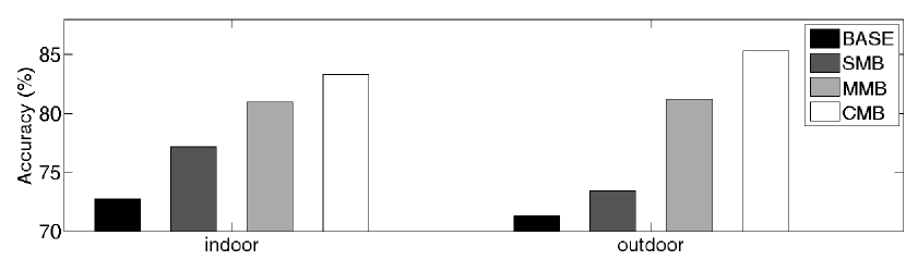
Figure 1: Performance comparison of different methods for indoor and outdoor scenes on development dataset of TUT16.

	GMM	NMF	CNN	BAS	SMB	MMB	CMB	VGG	HYB
eval.	77.2	87.7	86.2	-	-	86.4	88.7	83.3	89.7
dev.	72.5	86.2	79.0	72.24	75.65	80.8	83.9	79.5	89.9
rank	28	3	6	-	-	5	2	14	1

TABLE V: The accuracies on TUT16 dataset are provided for both evaluation set and development set. Also, we provide the ranks of each method for the DCASE-2016 challenge taken from the challenge’s website.

(%)	fold1	fold2	fold3	fold4	avg
BAS	78.97	64.48	68.46	77.5	72.24
SMB	84.14	68.28	75.17	75.00	75.65
MMB	85.86	76.55	77.52	83.22	80.79
CMB	87.93	80.34	81.54	85.62	83.86
VGG	80.69	75.52	77.85	83.90	79.49
HYB	94.48	85.17	87.25	92.81	89.93

TABLE VI: Accuracies of different methods on the development set cross-validation splits, provided with TUT16 dataset.

VII Results and Discussion

In Table V we present the results of our proposed methods and the baselines on the evaluation set and development set of TUT16. In addition, to provide a deeper insight, the performances of all the folds are reported separately in Table VI. To highlight the effectiveness of our multi-channel i-vector extraction scheme, a comparison between indoor and outdoor scene predictions are shown in Figure 1. To investigate the differences between the i-vector system and our CNN, the class-wise performances are provided in Table IV.

VII-A Performance comparison

As can be seen in Table V, on both the development and evaluation set, HYB has a better performance compared to all the baselines and proposed methods. Also CMB achieved the second best performance on the evaluation set and the third best performance on the development set. Comparing BAS with SMB, MMB and CMB shows that MFCC tuning, multi-channel i-vector extraction and score calibration improves the performance of the i-vector baseline step by step. Specially comparing BAS and CMB demonstrates the effectiveness of our multi-channel i-vector extraction scheme, improving BAS by 16 percentage points on the development set. This performance improvement is also visible in all the folds, as reported in Table VI. Comparing the CNN-based methods, CNN baseline performs better than our VGG-net. One reason could be in the use of mel-energy features rather than spectrograms which gives the CNN a benefit by having a more compact representation (60 dimension) compared to our spectrograms (149 dimensions). Between the feature learning methods (NMF, CNN and VGG), NMF achieved better performances on both development and evaluation set. And CMB outperformed all the other feature modeling techniques that used engineered features (GMM, BAS, SMB and MMB).

VII-B Improving I-vector Representation

As discussed in the introduction, one downside of i-vector features is their degradation in indoor scenes. In Figure 1 we demonstrated the overall performances for indoor scenes (Bus, Cafe, Car, Grocery store, Home, Library, Metro, Office, Train and Tram) and outdoor scenes (Beach, City center, Forest, Park and Residential area). Comparing BAS with SMB shows that our parameter tuning step improved both indoor and outdoor scene predictions. By looking at SMB and MMB we can observe that using multi-channel i-vector extraction scheme further improves the prediction performances. Finally, to study the effectiveness of our score calibration, we can compare the MMB and CMB. As can be seen, score calibration improves both indoor and outdoor scene predictions for i-vector systems.

VII-C VGG-net vs I-Vectors

Looking at Table IV, we can compare the performance of our best i-vector system with our VGG-net. Comparing CMB column with VGG column shows that for some of the classes, i-vector system performs better than VGG-net and for some other VGG-net achieves better prediction results. By looking at the HYB column we can observe that for most of the classes, the hybrid method performs better than both the i-vector and VGG-net. Only in the City and Tram classes the performance of the hybrid system is not better than VGG-net CNN and i-vector. Although it is not worse than the average of them in those cases, and its overall performance is better than both.

VII-D Final thoughts on our hybrid approach

Our experimental results support our hypothesis that i-vectors and CNNs provide complementary information from acoustic scenes. Hence, we can conclude that both of our feature learning method (CNN) and feature modeling based on engineered features (i-vector) system are capable of capturing acoustic events, enabling them to achieve promising performances in ASC. Studying the class-wise performances shows that each of these methods model the acoustic events differently from another. We provided a solution for combining the two modeling approaches by first create probability-like scores from each method and further fuse the scores. Our score fusion technique enables us to benefit from both methods, while minimizes the differences between the training and validation score distributions.

VIII Conclusion

In this paper, we investigated the parametrizations of MFCCs and provided a setup for MFCC extraction for ASC using i-vectors. We further proposed a novel multi-channel i-vector extraction scheme for ASC which uses different channels of the audio and significantly improves the performance of i-vector systems for ASC. We designed a VGG-style CNN architecture that achieves promising ASC results using spectrograms of audio segments. We investigated the differences between the features modeled based on engineered features (i-vectors) and a feature learning method (CNN), and showed they capture complementary information from acoustic scenes. Finally, we proposed a hybrid ASC system by fusing our multi-channel i-vectors with our VGG-net. Using our hybrid method, we achieved $1^{\text{st}}$ rank in the DCASE-2016 challenge [22] and using our multi-channel i-vector system we ranked $2^{\text{nd}}$.

References

- [1] X. Valero and F. Alias, “Gammatone cepst. coeffs: Biologically inspired features for non-speech audio classification,” Tran. on Mult., 2012.
- [2] N. Dehak, P. Kenny, R. Dehak, P. Dumouchel, and P. Ouellet, “Front-end factor analysis for speaker verification,” .
- [3] V. Bisot, R. Serizel, S. Essid, and G. Richard, “Acoustic scene classification with matrix factorization for unsupervised feature learning,” in ICASSP, 2016.
- [4] J. Salamon and J. P. Bello, “Deep cnns and data augmentation for environmental sound classification,” arXiv preprint, 2016.
- [5] H. Zeinali, L. Burget, H. Sameti, O. Glembek, and O. Plchot, “Dnns and hidden markov models in i-vector-based text-dependent speaker verification,” in Odyssey Workshop, 2016.
- [6] M. H. Bahari, R Saeidi, and D. Van Leeuwen, “Accent recognition using i-vector, gaussian mean supervector and gaussian posterior probability supervector for spontaneous telephone speech,” in ICASSP, 2013.
- [7] H. Eghbal-zadeh, B. Lehner, M. Schedl, and G. Widmer, “I-vectors for timbre-based music similarity and music artist classification,” in ISMIR, 2015.
- [8] B. Elizalde, H. Lei, G. Friedland, and N. Peters, “An i-vector based approach for audio scene detection,” DCASE workshop, 2013.
- [9] P. Kenny, “Joint factor analysis of speaker and session variability: Theory and algorithms,” Tech. Rep., 2005.
- [10] D. Garcia-Romero and C. Espy-Wilson, “Analysis of i-vector length normalization in speaker recognition systems.,” in INTERSPEECH, 2011.
- [11] S. Mika, G. Ratsch, J. Weston, B. Schölkopf, and K.-R. Muller, “Fisher discriminant analysis with kernels,” 1999.
- [12] A. O. Hatch, S. S. Kajarekar, and A. Stolcke, “Within-class covariance normalization for svm-based speaker recognition.,” in INTERSPEECH, 2006.
- [13] N. Dehak, R. Dehak, J. R. Glass, D. A. Reynolds, and P. Kenny, “Cosine similarity scoring without score normalization techniques.,” in Odyssey workshop, 2010.
- [14] B. Lehner, R. Sonnleitner, and G. Widmer, “Towards Light-weight, Real-time-capable Singing Voice Detection,” in ISMIR, 2013.
- [15] M. Brookes, “Voicebox: Speech Processing Toolbox for Matlab,” Website, 1999.
- [16] Min Lin, Qiang Chen, and Shuicheng Yan, “Network in network,” arXiv preprint, 2013.
- [17] N. Brümmer, “Focal multi-class: Toolkit for evaluation, fusion and calibration of multi-class recognition scores—tutorial and user manual—,” Tech. Rep., 2007.
- [18] L. Breiman, “Bagging predictors,” Machine learning, 1996.
- [19] A. Mesaros, T. Heittola, and T. Virtanen, “Tut database for acoustic scene classification and sound event detection,” in EUSIPCO, 2016.
- [20] V. Bisot, R. Serizel, S. Essid, and G. Richard, “Supervised nonnegative matrix factorization for acoustic scene classification,” Tech. Rep., DCASE2016 Challenge, 2016.
- [21] M. Valenti, A. Diment, G. Parascandolo, S. Squartini, and T. Virtanen, “Acoustic scene classification using convolutional neural networks,” Tech. Rep., DCASE2016 Challenge, 2016.
- [22] H. Eghbal-Zadeh, B. Lehner, M. Dorfer, and G. Widmer, “CP-JKU submissions for DCASE-2016: a hybrid approach using binaural i-vectors and deep cnns,” Tech. Rep., DCASE2016 Challenge, 2016.