Manipulating quantum coherence of charge states in interacting double-dot Aharonov-Bohm interferometers

Abstract

We investigate the dynamics of charge–states coherence in a degenerate double–dot Aharonov–Bohm interferometer with finite interdot Coulomb interactions. The quantum coherence of the charge states is found to be sensitive to the transport setup configurations, involving both the single–electron impurity channels and the Coulomb–assisted ones. We numerically demonstrate the emergence of a complete coherence between the two charge states, with the relative phase being continuously controllable through the magnetic flux. Remarkably, a fully coherent charge qubit arises at the double–dots electron pair tunneling resonance condition, where the chemical potential of one electrode is tuned at the center between a single–electron impurity channel and the related Coulomb–assisted channel. This pure quantum state of charge qubit could be experimentally located at the current–voltage characteristic turnover position, where differential conductance sign changes. We further elaborate the underlying mechanism for both the real–time and the stationary charge–states coherences in the double–dot systems of study.

I Introduction

The investigations of semiconductor quantum dots have long aroused a great deal of attentions. The various controllability of quantum dots, in terms of not only the geometric shape and size but also the internal energy levels and couplings, make it particularly useful in serving as good testbeds for the study of mesoscopic physics, as well as in potential applications for nanotechnology and quantum information processing. Especially, quantum dots are the promising candidates for the realizations of scalable quantum computer, implemented with the electron charge and/or spin qubits. Kan98133 ; Los98120 ; Han071217 ; Hay03226804 ; Fuj06759 Much progress has been made for the investigation of quantum coherence dynamics, in particular, the manipulation of charge–state coherence in the lateral double–dot systems. Hay03226804 ; Fuj06759 ; Tu08235311 ; Pet10246804 ; Dov11161302 ; Cao131401 ; Kim15243

On the other hand, quantum coherence transport through parallel double–dots embedded in Ahronov–Bohm (AB) interferometers has also been extensively studied both experimentally Sch97417 ; Hol01256802 ; Sig06036804 ; Hat11076801 and theoretically. Ent02166801 ; Kon013855 ; Kon02045316 ; Li09521 ; Har13235426 ; Tok07113 ; Szt07386224 ; Bed14235411 ; Bed12155324 ; Bed13045418 ; Rep16165425 ; Pul10256801 ; Tu11115318 ; Tu12115453 ; Liu16045403 The particular interest in a ring–structured AB interferometer is the electron interference which can be tuned by an externally applied magnetic flux. The resulted coherent transport property has been characterized via conductance oscillation in magnetic flux. Hol01256802 ; Sig06036804 It has been widely studied in quantum transport the relation of the coherence of AB oscillations to Coulomb interaction, Kon013855 ; Kon02045316 ; Li09521 ; Har13235426 ; Tok07113 ; Bed14235411 ; Szt07386224 interdot tunneling,Szt07386224 ; Hat11076801 and inelastic electron cotunneling processes, Sig06036804 ; Rep16165425 etc. However, the coherent dynamics of the AB double-dot charge states has not yet been explored in depth when the Coulomb interaction is fully taken into account because of the theoretical difficulty. Preliminary studies demonstrated that the intrinsic dynamics of charge states would display just a phase localization rather than coherence in a symmetric geometry setup, Tu11115318 ; Bed12155324 unless an asymmetrical geometrical setup is arranged Tu12115453 or a large Coulomb interaction is included. Tok07113 ; Bed12155324

In this work, we study the coherence dynamics of charge states in double–dot AB interferometers, in the presence of finite interdot Coulomb interaction. The analysis is carried out based on the well–established nonperturbative hierarchical equations–of–motion (HEOM) approach.Jin08234703 ; Li12266403 ; Ye16608 The quantum coherence of charge states is shown to be sensitive to the transport regimes of the electron tunneling channels, including single–electron impurity channels and Coulomb ones in double dots. We find that AB double–dots, with finite interdot Coulomb interaction, would be very suitable for the preparation of a fully coherent charge qubit. The relative phase of the charge qubit is continuously controllable through the magnetic flux, rather than the phase localization, as studied previously on the weak or noninteracting counterparts.Tu11115318 ; Bed12155324 In particular, a fully coherent charge qubit emerges at the double–dots electron pair tunneling resonance, when the chemical potential of one electrode matches with the center between a single–electron impurity channel and the related Coulomb channel. This pure quantum state of charge quit could be experimentally located at the current–voltage characteristic turnover position, where differential conductance changes sign, from negative (positive) to positive (negative). Finally, using a transformation to reformulate the problem, we elaborate the underlying mechanism for the real–time dynamics of the nonequilibrium charge–states coherence from weak to strong interdot Coulomb interactions.

The rest of paper is organized as follows. In Sec. II, we introduce the standard transport model of the double–dot AB interferometers and briefly outline the HEOM approach for describing the coherence dynamics of the charge states in the double-dot. In Sec. III, we present the converged stationary results on the quantum coherence of the charge qubit in different tunneling regimes, in the presence of finite interdot Coulomb interaction. We then study the real–time dynamics and elaborate the underlying mechanism of the observed nonequilibrium charge-states coherence in Sec. IV. Finally, we give the summary in Sec. V.

II Methodology

Consider the nonequilibirum electron transport through a parallel double-dot embedded in an AB interferometer, its total Hamiltonian, $H_{\mbox{\tiny T}}=H_{\mbox{\tiny S}}+H_{\mbox{\tiny B}}+H_{\mbox{\tiny SB}}$, consists of three parts. The central parallel double-dot system is modeled by

$$H_{\mbox{\tiny S}}=\sum_{u=1,2}\varepsilon_{u}\hat{n}_{u}+U\hat{n}_{1}\hat{n}_{2},\ \ \text{with}\ \ \hat{n}_{u}=a^{\dagger}_{u}a_{u}.$$ (1)

Here, $a_{u}$ ($a^{\dagger}_{u}$) denotes the annihilation (creation) operator of the electron in the dot-$u$ orbital state of energy $\varepsilon_{u}$, and $U$ is the interdot Coulomb interaction. The electrodes are modeled as noninteracting electrons reservoirs bath, i.e.,

$$H_{\mbox{\tiny B}}=\sum_{\alpha k}(\epsilon_{\alpha k}+\mu_{\alpha})c^{\dagger}_{\alpha k}c_{\alpha k}$$ (2)

with $\alpha=L,R$, under the applied bias voltage potential $eV=\mu_{L}-\mu_{R}$. Here, $c^{\dagger}_{\alpha k}$ ($c_{\alpha k}$) denotes the creation (annihilation) operator of the electron with momentum $k$ in the specified $\alpha$-reservoir. The electrons tunneling between the dots and the reservoirs is described by the tunneling Hamiltonian,

$$H_{\mbox{\tiny SB}}=\sum_{\alpha uk}\left(e^{i\phi_{\alpha u}}t_{\alpha uk}a^{\dagger}_{u}c_{\alpha k}+{\rm H.c.}\right),$$ (3)

with the AB flux $\Phi$–induced phase factors satisfying

$$\phi_{L1}-\phi_{L2}+\phi_{R2}-\phi_{R1}=\phi\equiv 2\pi\Phi/\Phi_{0}.$$ (4)

Here, $\Phi_{0}$ denotes the flux quantum. Without loss of generality, we adopt (due to the gauge invariant)Tu11115318 ; Bed13045418

$$\phi_{L1}=-\phi_{L2}=\phi_{R2}=-\phi_{R1}=\phi/4.$$ (5)

The hybridization spectral function assumes Lorentzian,

$$J_{\alpha uv}(\omega) \equiv\pi e^{i(\phi_{\alpha v}-\phi_{\alpha u})}\sum_{k}t^{\ast}_{\alpha uk}t_{\alpha vk}\delta(\omega-\epsilon_{\alpha k})$$

$$=\frac{\Gamma_{\alpha uv}W^{2}}{\omega^{2}+W^{2}},$$ (6)

with the equal coupling strengths,

$$\begin{split}\Gamma_{\alpha 11}&=\Gamma_{\alpha 22}=\Gamma/2,\\ \Gamma^{\ast}_{L12}&=\Gamma_{L21}=\Gamma_{R12}=\Gamma^{\ast}_{R21}=e^{i\phi/2}\Gamma/2.\end{split}$$ (7)

Throughout this work, we set the unit of $e=\hbar=1$, for the electron charge and the Planck constant. In numerical calculations we set $\mu_{L}=-\mu_{R}=V/2$ and fix the bandwidth at $W=10$ meV for electrodes.

In close contact to experiments,Fuj06759 ; Han071217 we set the spinless double–dots to be degenerate, i.e., $\varepsilon_{1}=\varepsilon_{2}=\varepsilon$ in Eq. (1). The optimized coherence would then be anticipated. The involved states in the double dots are $|0\rangle=|00\rangle$, $|1\rangle=|10\rangle$, $|2\rangle=|01\rangle$, and $|d\rangle\equiv|11\rangle$, i.e., the empty, the dot-$1$ occupied, the dot-$2$ occupied, and double–dots–occupancy states, respectively. The quantum coherence properties of the double–dots states are described by the reduced system density matrix, $\rho(t)\equiv{\rm tr}_{\mbox{\tiny B}}\rho_{\rm tot}(t)$, i.e., the partial trace of the total density operator $\rho_{\rm tot}$ over the electrode bath degrees of freedom.

We implement the celebrated HEOM formalism,Jin08234703

$$\dot{\rho}^{(n)}_{\bf j}(t) =-\bigg{(}i{\cal L}_{\mbox{\tiny S}}+\sum_{r=1}^{n}\gamma_{j_{r}}\bigg{)}\rho^{(n)}_{\bf j}(t)-i\sum_{j}{\cal A}_{\bar{j}}\rho^{(n+1)}_{{\bf j}j}(t)$$

$$\quad-i\sum_{r=1}^{n}(-)^{n-r}{\cal C}_{j_{r}}\rho^{(n-1)}_{{\bf j}^{-}_{r}}(t),$$ (8)

to accurately evaluate the real–time dynamics of the reduced system density matrix, $\rho^{(0)}(t)\equiv\rho(t)$, whereas $\rho^{(n)}_{\bf j}(t)\equiv\rho^{(n)}_{j_{1}\cdots j_{n}}(t)$, with $\rho^{(n<0)}(t)\equiv 0$. In Eq. (II), ${\cal L}_{\mbox{\tiny S}}\,\cdot\,\equiv[H_{\mbox{\tiny S}},\,\cdot\,]$ defines the reduced system Liouvillian; $j\equiv(\sigma,\alpha,u,\kappa)$ and $\bar{j}\equiv(\bar{\sigma},\alpha,u,\kappa)$ denote the specified collective indexes. Here, $\sigma=+,-$, and $\bar{\sigma}$ is its opposite sign; $\kappa$ arises from the nonequilibrium interacting reservoirs bath correlation functions,Jin08234703 ; Li12266403 ; Ye16608 ; Hu10101106 ; Hu11244106 in an exponent expansion form of $C^{\sigma}_{\alpha uv}(t)=\sum_{\kappa=1}^{K}\eta^{\sigma}_{\alpha uv\kappa}e^{-\gamma^{\sigma}_{\alpha\kappa}t}$. Together with denoting $a^{+}_{u}\equiv a^{\dagger}_{u}$, and $a^{-}_{u}\equiv a_{u}$, the Grassmannian superoperators, ${\cal A}_{\bar{j}}\equiv{\cal A}^{\bar{\sigma}}_{\alpha u\kappa}={\cal A}^{\bar{\sigma}}_{u}$ and ${\cal C}_{j}\equiv{\cal C}^{\sigma}_{\alpha u\kappa}$ in Eq. (II), are defined viaJin08234703 ; Li12266403 ; Ye16608

$$\begin{split}{\cal A}^{\sigma}_{u}\hat{O}_{\mbox{\tiny$\pm$}}&\equiv a^{\sigma}_{u}\hat{O}_{\mbox{\tiny$\pm$}}\pm\hat{O}_{\mbox{\tiny$\pm$}}a^{\sigma}_{u}\equiv\big{[}a^{\sigma}_{u},\hat{O}_{\mbox{\tiny$\pm$}}\big{]}_{\pm}\,,\\ {\cal C}^{\sigma}_{\alpha u\kappa}\hat{O}_{\mbox{\tiny$\pm$}}&\equiv\sum_{v}\big{(}\eta^{\sigma}_{\alpha uv\kappa}a^{\sigma}_{v}\hat{O}_{\mbox{\tiny$\pm$}}\mp\eta^{\bar{\sigma}\,{\ast}}_{\alpha uv\kappa}\hat{O}_{\mbox{\tiny$\pm$}}a^{\sigma}_{\kappa}\big{)}.\end{split}$$ (9)

Here, $\hat{O}_{\mbox{\tiny$\pm$}}$ denotes an arbitrary operator, with even ($+$) or odd ($-$) fermionic parity, such as $\rho^{(2m)}$ or $\rho^{(2m+1)}$, respectively.

The stationary solutions to HEOM (II) can be obtained by using the conditions, $\{\dot{\rho}^{(n);{\rm st}}_{\bf j}=0;\forall n\}$. These together with the normalization constraint, ${\rm tr}\rho^{(0)}=1$, lead to Eq. (II) a set of coupled linear equations for solving $\{\dot{\rho}^{(n);{\rm st}}_{\bf j}=0\}$. In practical calculations, an iterative quasiminimal residual algorithmFre91315 ; Ste07195115 is employed for solving the large–sized coupled linear equations.Ye16608 Equation (II) can also be called the dissipaton equation of motion (DEOM).Yan14054105 ; Jin15234108 ; Yan16110306 The latter is a quasi–particle theory, which identities the physical meaning of individual $\rho^{(n)}_{\bf j}(t)\equiv\rho^{(n)}_{j_{1}\cdots j_{n}}(t)$. Besides Eq. (II), the DEOM theory includes also the underlying disspaton algebra, especially the generalized Wick’s theorem.Yan14054105 ; Jin15234108 ; Yan16110306 This extends the real–time dynamics further to the interacting bath subspace. Not only the transient transport current,Zhe08184112 ; Zhe08093016 ; Wan13035129 but also the nonequilibrium current–current correlation functions can then be evaluated.Jin15234108

As a nonperturbative theory, HEOM usually converges rapidly and uniformly.Li12266403 ; Ye16608 ; Zhe09164708 ; Hou15104112 The hierarchy can be terminated simply by setting all $\rho^{(n>L)}_{\bf j}=0$, at a sufficiently large $L$. For the AB double–dot system exemplified in this work, the HEOM evaluations effectively converge at the $L=3$ tier level.

III Coherence of charge qubit

III.1 Coherence control with bias voltage

We focus on the quantum coherence of the two charge states, $\{|1\rangle,|2\rangle\}$, which constitute a charge qubit, with the single–electron occupation. The interested charge–qubit density operator $\rho_{e}(t)$ is the $2\times 2$ sub-matrix of the reduced system $\rho(t)$. The latter and also other $\rho^{(n)}_{\bf j}(t)$ spans over all the four Fock states, $\{|0\rangle,|1\rangle,|2\rangle,|d\rangle\}$. The probability of single electron occupation is given by $p_{e}={\rm tr}\rho_{e}=\rho_{11}+\rho_{22}\leq 1$. The nonzero probabilities of the empty and double–occupation states, $\rho_{00}$ and $\rho_{dd}$, are the leakage effects. Tu11115318 ; Jin13064706 Denote $\delta=\rho_{11}-\rho_{22}$ for the probability difference between the two charge states. The charge qubit entropy is given by $S_{e}=-{\rm tr}(\varrho_{e}\ln\varrho_{e})$, with $\varrho_{e}=\rho_{e}/{\rm tr}(\rho_{e})$ and $S^{\text{max}}_{e}=\ln 2$ for two–level systems. Thus $\chi_{e}=1-S_{e}/\ln 2$, satisfying $0\leq\chi_{e}\leq 1$, can be used a purity measure, with $\chi_{e}=1$ indicating a truly pure state of the charge qubit.

Figure 1 reports the nonequilibrium steady–state results, as functions of the applied voltage, on the charge–quit state properties given in (a) and (b), the leakage effects in (c), and the transport current in (d), respectively, where the Coulomb interaction of $U=0.5$ meV and the AB phase of $\phi=\pi/2$ are used, see the description in the figure caption for the details.

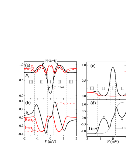
Figure 1: (Color online) The accurate results for the stationary charge state varying with bias voltage $V$ through different tunneling regimes at the fixed flux $\phi=\pi/2$ and Coulomb interaction $U=0.5{\rm meV}$. (a) The probability of single-electron occupation and the purity measurement of the resulted charge qubit (the solid lines for the weak tunneling rate $\Gamma=0.02{\rm meV}$, and the dashed lines for the strong tunneling rate $\Gamma=0.1{\rm meV}$). (b) The probability difference ($\delta$ ) between the two charge states and their coherence term ($\rho_{12}$). (c) The leakage effects of the probabilities of the empty and the double occupation states. (d) The average current (the gray-line for noninteracting system $U=0$). The other parameters are $k_{\mbox{\tiny B}}T=0.02{\rm meV}$, $\varepsilon=0.1{\rm meV}$, and $\Gamma=0.02{\rm meV}$ for (b)-(c).

The observed results can be understood in terms of the interplay between different tunneling channels involved in individual transport regimes. First of all, there are two types of tunneling channels: The single-electron impurity channels with the degenerate energy levels at $\varepsilon_{1}=\varepsilon_{2}=\varepsilon$, and the Coulomb–assisted channels at $\varepsilon+U$. Concerning further their positions in relation to the applied voltage window, we identify three transport regimes, indicated in Fig. 1 in terms of I, II, and III, respectively. Let us start with the double–dots state versus voltage, the $\rho$-$V$ characteristics, reported in Fig. 1(a)–(c).

$\bullet\ \,$Regime I: $\varepsilon+U>\varepsilon>\mu_{R(L)}$. This is the cotunneling regime, with the bias window containing no tunneling channels. The resulted single–electron occupation ($p_{e}=\rho_{11}+\rho_{22}$) and double occupation ($\rho_{dd}$) are both negligible. The full probability of empty state ($\rho_{00}$) emerges.

$\bullet\ \,$Regime II: $\varepsilon+U\!>\!\mu_{L(R)}\!>\!\varepsilon\!>\!\mu_{R(L)}$. This is the Coulomb–blockade (CB) regime, and is of particular interest in the present work. The most striking scenario occurs at the bias voltage of $|V|=2\varepsilon+U$. There emerges a nearly pure charge qubit state, with the single–electron occupation, $p_{e}=\rho_{11}+\rho_{22}$, and the purity parameter, $\chi_{e}$, being both in close proximity to their maximum values of 1. These results are specified with the arrows on the solid curves in Fig. 1 (a), where $\Gamma=0.02$ meV and $k_{B}T=0.02$ meV are adopted for demonstration. At $|V|=2\varepsilon+U$, while $\rho_{00}+\rho_{dd}=1-p_{e}\simeq 0$, we have also $\delta=\rho_{11}-\rho_{22}=0$ and therefore $|\rho_{12}|\simeq 0.5$, as seen in Fig. 1 (b) and (c). The dashes curves in Fig. 1 (a) goes with the increased lead coupling strength, $\Gamma=0.1$ meV. Apparently, increasing temperature also decreases the purity of the charge qubit state. Note that in the present symmetric bias setup, $|V|=2\varepsilon+U$ amounts actually to the pair tunneling resonance condition,Lei09156803 which would also occur in the Coulomb participated regime (II^′), where $\mu_{L}>\varepsilon+U>\mu_{R}>\varepsilon$; see Sec. III.2 for the details.

$\bullet\ \,$Regime III: $\mu_{L(R)}\!>\!\varepsilon,\varepsilon+U\!>\!\mu_{R(L)}$. This is the sequential-dominated regime, as both the single–electron impurity and Coulomb–assisted tunneling channels fall inside the bias window. The results here are similar to those of $U=0$ and weak $U$ obtained in Refs. Bed12155324, and Tu11115318, , respectively. Indeed, as reported there before, the localization of the phase, $\theta=\arctan[{\rm Im}(\rho_{12})/{\rm Re}(\rho_{12})]$, appears at the value of $\theta=-\pi/2$ or $\pi/2$. Either of these two values corresponds to ${\rm Re}\,\rho_{12}=0$ [cf. Fig. 1 (b)]. The fact that ${\rm Re}\,\rho_{12}$ vanishes in the sequential-dominated regime (III) is rather robust against the flux; see the discussion for Fig. 2 later.

Figure 1 (d) depicts the current-voltage ($I$-$V$) characteristics. Particularly, in the CB regime (II) that does not exist for noninteracting ($U=0$; grey–curve) case, the $I$-$V$ curve exhibits a remarkable concave down (or up) feature, for $V>0$ (or $V<0$). The turnover positions, located with the arrows in Fig. 1 (d), are right at $|V|=2\varepsilon+U$. In other words, the nearly pure charge qubit state, with both the purity and occupation number parameters, $\chi_{e}$ and $p_{e}$ [see Fig. 1 (a)], in close proximity to their maximum values of 1, could be experimentally located at the aforementioned $I$-$V$ characteristic turnover position, where the differential conductance sign changes.

III.2 Charge qubit phase at pair transfer resonance versus Aharonov-Bohm magnetic flux

Examine now $\theta=\arctan[{\rm Im}(\rho_{12})/{\rm Re}(\rho_{12})]$, the charge qubit phase, as functions of the magnetic flux. We focus on the case of $V=|2\varepsilon+U|$, at which the charge qubit is in close proximity to a pure state; cf. Fig. 1(a). It is noticed that in the present symmetric bias setup, $V=|2\varepsilon+U|$ satisfies the pair tunneling resonance condition,Lei09156803

$$\mu_{\alpha}-\varepsilon=\varepsilon+U-\mu_{\alpha}.$$ (10)

Beside the CB regime (II) described earlier, the pair tunneling occurs also in another transport setup configuration:
$\bullet\ \,$Regime II^′: $\mu_{L}>\varepsilon+U>\mu_{R}>\varepsilon$, the Coulomb participation (CP) regime. In this regime, the transport would be primarily driven by the electron tunneling from dots to $R$-lead. The relevant pair tunneling resonance is therefore Eq. (10) with $\alpha=R$. On the other hand, in the CB regime (II), where $\varepsilon+U>\mu_{L}>\varepsilon>\mu_{R}$, the resonance follows Eq. (10) with $\alpha=L$, as the transport would now be primarily driven by the electron tunneling from $L$-lead to dots.

Figure 2 reports the nonequilibrium steady–state results, as functions of the applied AB magnetic flux, in terms of $\phi/\pi\equiv 2\Phi/\Phi_{0}$. Both the CB (black–curves) and CP (green–curves) cases are operated at the pair tunneling resonance voltage, $V=|2\varepsilon+U|=0.7$ meV, with the same $U=0.5$ meV, but different values of $\varepsilon=0.1$ meV and $-0.6$ meV, respectively. Included for comparison are also the sequential-dominated regime (III) counterparts (red–dashed–curves), exemplified with $U=0.1$ meV and $\varepsilon=0.1$ meV at $V=0.7$ meV. As that in Fig. 1, where $\phi=\pi/2$, the sequential-dominated regime displays the phase localization at $\theta=-\pi/2$ or $\pi/2$, for $V<0$ and $V>0$, respectively.Tu11115318 This result is independent of the flux at $\phi\neq 2m\pi$, with $m$ being an integer, as shown by the red–dashed horizontal parts in Fig. 2 (a), where Re $\rho_{12}=0$, see Fig. 2 (b). The single–electron occupation, $p_{e}$, and the leakage effects, $\rho_{00}$ and $\rho_{dd}$, as shown by the red–dashed curves in Fig. 2 (d)–(f), also agree with those noninteracting ($U=0$) results reported in Ref. Tu11115318, .

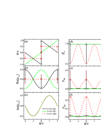
Figure 2: (Color online) The accurate results for the stationary charge state varies with the magnetic flux for different Coulomb interaction at the bias voltage $V=0.7{\rm meV}$. (a) The characteristic coherence is denoted by the relative phase $\theta$, and (b) and (c) the real and imaginary parts of $\rho_{12}$. The probabilities of the states for single-electron occupation, empty, and double occupation are illustrated in (d), (e), and (f), respectively. Here, $U=0.1$ meV is for sequential-dominated regime (III), and $U=0.5$ meV is for CB regime (II) (black–curves, where $\varepsilon=0.1$ meV) and CP regime (II^′) (green–curves, where $\varepsilon=-0.6$ meV) with satisfying $V=|2\varepsilon+U|$. The other parameters are the same as in Fig. 1.

On the other hand, in both the CB (II) and CP (II^′) regimes, while ${\rm Im}\rho_{12}$ is rather independent of the interdot Coulomb coupling, ${\rm Re}\rho_{12}$ significantly deviates from the zero-value behavior in the $U=0$ case. The single–electron occupation is remarkably enhanced, and meanwhile the leakage effects are greatly suppressed. Especially, at $|V|=|2\varepsilon+U|$ that satisfies the pair tunneling resonance condition,Lei09156803 the charge qubit state, as inferred from Fig. 1(a) and (b) for its $\chi_{e}\simeq 1$ and $\delta\equiv\rho_{11}-\rho_{22}=0$, assumes a pure–state proximity of

$$|\psi\rangle=\frac{1}{\sqrt{2}}\big{(}|1\rangle+e^{-i\theta}|2\rangle\big{)}.$$ (11)

The AB magnetic flux–tuned phase, as shown in Fig. 2 (a) for $V>0$, is given by

$${\theta}=\begin{cases}\pi-\phi/2;&\text{CB regime (II)}\\ \phi/2;&\text{CP regime (II${}^{\prime}$)}\end{cases}.$$ (12)

For the bias $V<0$, the above relations hold with exchange of $\phi$ to $-\phi$ (not shown in Fig. 2), due to the phase–lead symmetry relations underlying Eq. (5).

Remarkably, as shown in Fig. 2, while the singularity occurs in the CB regime (II) at $\phi=2m\pi$, the CP counterparts are completely free of the singularity. The nearly pure charge qubit state, with both the purity parameter, $\chi_{e}$, and occupation number, $p_{e}$, in close proximity to their maximum values of 1. It is interesting to notice that in the present CP regime (II^′) setup, the double–occupation level locates below the transport window; i.e., $\epsilon_{d}=2\varepsilon+U=-0.7\,\text{meV}<\mu_{R}=-0.35\,\text{meV}$ in study. However, its occupation number $\rho_{dd}$ remains very small, under the pair tunneling resonance voltage; see Fig. 2 (f). Involved here is also the interference resonance that overcomes the leakage from the desired charge qubit state.

IV Coherence dynamics analysis

IV.1 Charge qubit coherence dynamics

To further explore the underlying machnism of the full coherence realization of the charge qubit states in the AB interferometers, we study the evolution of $\rho_{12}(t)$, the transient charge–qubit coherence, in both the CB regime (II) (left–panels) and the CP regime (II^′) (right–panels), with the initial empty state in the double dots ($\rho_{00}(0)=1$). The results are presented in Fig. 3. It shows that the short-time ($t\lesssim 1/\Gamma$) dynamics in both the regime II and II^′ are quite similar as that in the sequential-dominated regime (III) reported previously in Refs. Bed12155324, and Tu11115318, . The short-time dynamics of $\rho_{12}(t)$ is dominated by the electron tunneling through the single–electron impurity channels ($\varepsilon$), with little contributions from the Coulomb–assisted channel ($\varepsilon+U$). Denote $\rho_{12}(t)=|\rho_{12}(t)|e^{i\theta(t)}$, the relative phase between the two charge states, $|1\rangle$ and $|2\rangle$, is found to be $\theta(t)=\phi/2$ when $t\lesssim 1/\Gamma$. For $t>1/\Gamma$, the charge–qubit coherence becomes sensitive to the specific tunneling regimes. The relative locations of the single–occupation ($\varepsilon$) and the double–occupation ($\varepsilon+U$) transport channels with respect to the bias window take the crucial role when $t>1/\Gamma$. Especially the nonequilibrium charge qubit operated in either the CB regime (II) or the CP regime (II^′) remains a proximity to a full coherence dynamics, as shown by Eq. (11) in the long–time limit. The characteristics of Im $\rho_{12}(t)$ are similar in these two transport regimes, without changing signs as the time evolves, while Re $\rho_{12}(t)$ behaviors differ remarkably. In the CB regime (II) (see Fig. 3 (a)), Re $\rho_{12}(t)$ will switch the sign (unless $\phi=2m\pi$ that is associated with $\theta=\pi/2$ for $V>0$), which leads to the relative phase $\theta=\pi-\phi/2$. On the other hand, in the CP regime (II^′), as shown in Fig. 3 (b), Re $\rho_{12}(t)$ has no such sign change and the relative phase remains as the case of $\theta(t)=\phi/2$. Note that the above results in the CB regime and the CP regime could be changed significantly by weakening the Coulomb interaction or increasing the bias voltage or temperature. For example, the full coherence of charge qubit dynamics would be immediately broken down and the charge qubit state is reduced to the phase localization, similar to the noninteracting ($U=0$) limit in the previous studies.Tu11115318 ; Bed12155324

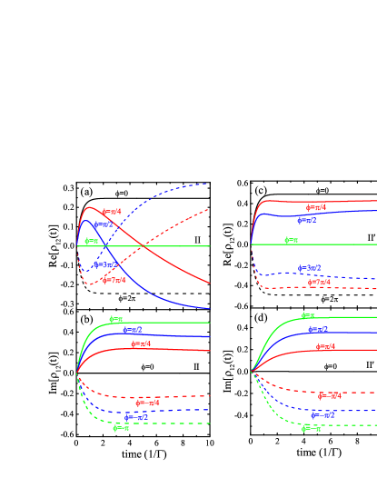
Figure 3: (Color online) The coherence evolution of $\rho_{12}(t)$ for CB regime (II) ($\varepsilon=0.1$ meV) and the CP regime (II^′) ($\varepsilon=-0.6$ meV) setups in the left (a and b) and right (c and d) panels, respectively, with the strong interdot Coulomb interaction $U=0.5$ meV. The other parameters are the same as in Fig. 2.

IV.2 Mechanistic analysis

The above nonequilibirum features on the charge–states coherence dynamics, including the short–time, long–time and stationary state behaviors, can be understood as follows. Taking the following transformation on the electron operators in the dots,

$$\tilde{a}_{1}=({a}_{1}+{a}_{2})/{\sqrt{2}}\ \ \text{and}\ \ \tilde{a}_{2}=({a}_{1}-{a}_{2})/{\sqrt{2}}.$$ (13)

The system and bath Hamiltonians, Eqs. (1) and (2), are invariant under this transformation. The tunneling Hamiltonian, Eq. (3), becomes

$${\widetilde{H}}_{\mbox{\tiny SB}}=\sum_{\alpha uk}\left({\tilde{t}}_{\alpha uk}{\tilde{a}}^{\dagger}_{u}c_{\alpha k}+{\rm H.c.}\right),$$ (14)

with ${\tilde{t}}_{\alpha 1k}=\sqrt{2}\,t_{\alpha 1k}\cos(\phi/4)$ and ${\tilde{t}}^{\ast}_{L2k}={\tilde{t}}_{R2k}=i\sqrt{2}\,t_{\alpha 2k}\sin(\phi/4)$. The above results are schematically depicted in Fig. 4. The transformed hybridization spectral function, with the equal coupling strengthes of Eq. (7), remain the Lorentzian form of Eq. (II), but having

$$\begin{split}\widetilde{\Gamma}_{\alpha 11}&=2\Gamma\cos^{2}(\phi/4),\ \ \ \widetilde{\Gamma}_{\alpha 22}=2\Gamma\sin^{2}(\phi/4),\\ \widetilde{\Gamma}_{L21}&=\widetilde{\Gamma}^{\ast}_{L12}=\widetilde{\Gamma}_{R12}=\widetilde{\Gamma}^{\ast}_{R21}=i\,\Gamma\sin(\phi/2).\end{split}$$ (15)

From $|u\rangle=a^{\dagger}_{u}|0\rangle$ and $|\tilde{u}\rangle=\tilde{a}^{\dagger}_{u}|0\rangle$ with Eq. (13), we have

$$\begin{split}\rho_{11}&=\left(\rho_{\tilde{1}\tilde{1}}+\rho_{\tilde{2}\tilde{2}}+2\,{\rm Re}\,\rho_{\tilde{1}\tilde{2}}\right)/2,\\ \rho_{22}&=\left(\rho_{\tilde{1}\tilde{1}}+\rho_{\tilde{2}\tilde{2}}-2\,{\rm Re}\,\rho_{\tilde{1}\tilde{2}}\right)/2,\\ \rho_{12}&=\left(\rho_{\tilde{1}\tilde{1}}-\rho_{\tilde{2}\tilde{2}}-2i\,{\rm Im}\,\rho_{\tilde{1}\tilde{2}}\right)/2.\end{split}$$ (16)

Equations (15) and (16) are used in the following analysis, with the focus on the flux $\phi$–dependent charge qubit phase, $\theta=\arctan[{\rm Im}(\rho_{12})/{\rm Re}(\rho_{12})]$.

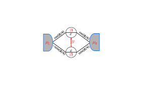
Figure 4: (Color online) The schematic view of a double-dot AB interferometer in the new basis in terms of the transformation Eq. (13) and the corresponding tunneling Hamiltonian of Eq. (14).

Let us start with the two special scenarios, where the interdot Coulomb interaction does not play the role, and the charge qubit phases are always localized.

(i) At $\phi=2m\pi$, we have $\theta=0$ or $\pi$ (cf. the black–lines in Fig. 3). As inferred from Eq. (15), this scenario has either $\widetilde{\Gamma}_{\alpha 11}=0$ or $\widetilde{\Gamma}_{\alpha 22}=0$, with odd or even $m$, respectively, and also $\widetilde{\Gamma}_{\alpha 12}=0$. The electron tunnels through only one of the transformed single–occupation channels, either $|\tilde{2}\rangle$ or $|\tilde{1}\rangle$. Consequently, $\rho_{\tilde{1}\tilde{2}}=0$, since there is no interference between these two states. In this case, $\rho_{12}(t)$ is always real, as inferred from Eq. (16), and the charge qubit phase is localized at $\theta=0$ or $\pi$. Physically the above scenario amounts to the transport setup involving only one single spinless electronic level. The interdot Coulomb interaction does not play any roles in this scenario, and the double–occupation is always $p_{d}(t)=0$. The long–time probabilities of the empty and the single-electron occupied states are equal, i.e., $p_{0}=0.5$ and $p_{e}=0.5$. The latter is via either $\rho_{\tilde{1}\tilde{1}}$ or $\rho_{\tilde{2}\tilde{2}}$, exclusively.

(ii) At $\phi=(2m+1)\pi$, we have $\theta=\pm\pi/2$ (cf. the green–lines in Fig. 3). As inferred from Eq. (15), this scenario goes by $\widetilde{\Gamma}_{\alpha 11}=\widetilde{\Gamma}_{\alpha 22}=|\widetilde{\Gamma}_{\alpha 12}|=\Gamma/2$, resulting in $\rho_{\tilde{1}\tilde{1}}(t)=\rho_{\tilde{2}\tilde{2}}(t)=|\rho_{\tilde{1}\tilde{2}}(t)|$. This is the case of a full interference with equal probability. In this case, $\rho_{12}(t)$ is always pure imaginary, as inferred from Eq. (16), and the charge qubit phase is localized at $\theta=\pm\pi/2$. Physically, a full interference with equal probability is an interference resonance. It leads to the maximum value of $p_{e}=\rho_{11}+\rho_{22}\approx 1$ in the long–time region. Both the vacancy and double occupations are suppressed. This interference resonance behavior is independent of interdot Coulomb interaction.

Turn to the situations of $\phi\neq n\pi$, away from the above two special scenarios, and the interdot Coulomb interaction will play the roles. The general remarks on the nonspecial situations are as follows. (a) In the short–time ($t>1/\Gamma$) region, electrons tunnel mainly through two single-electron impurity channels, with $\varepsilon_{\tilde{1}}=\varepsilon_{\tilde{2}}=\varepsilon$. According to the flux–dependent tunneling rate of Eq. (15), one of them could be called the fast channel and the other be the slow one.Saf03136801 More precisely, $|\tilde{1}\rangle$ is the fast channel when $\phi<\pi/4$, whereas it is the slow one when $\phi>\pi/4$. The fast channel dominates in short time. The above analysis also dictates the sign of ${\rm Re}[\rho_{12}(t)]=[\rho_{\tilde{1}\tilde{1}}(t)-\rho_{\tilde{2}\tilde{2}}(t)]/2$ [cf. Eq. (16)] in the short time region. As time evolves, the slow channel occupation gradually accumulates. The sign of ${\rm Re}[\rho_{12}(t)]$ would change if the population inversion could occur. For example, the individual curve in Fig. 3(a) changes sign, while that in Fig. 3(c) does not. We will elaborate these observations later; (b) When $t>1/\Gamma$, Coulomb–assisted ($\varepsilon+U$)-channels play roles. These are the transfer channels, rather than the double–occupation state of energy $2\varepsilon+U$.

Focus hereafter the long–time behavior for $\phi\neq n\pi$, which depends on both single–electron $\varepsilon$–channel and Coulomb–assisted ($\varepsilon+U$)–channel. Apparently, the nonequilibrium property manifests the interplay between these two transfer channels and their relative locations with respect to the bias window. The cotunneling regime (I) is not the interest of this work, since it generates no significant population in the charge qubit state. On the other hand, the sequential–dominant regime (III), where $\mu_{L}>\varepsilon,\varepsilon+U>\mu_{R}$, the interested transfer channels both fall inside the bias window. This is similar to the well–studied Coulomb–free scenario,Bed12155324 ; Tu11115318 with the results being summarized as follows. In the wide–band–reservoirs limit, the probabilities of electrons tunneling through $|\tilde{1}\rangle$ and $|\tilde{2}\rangle$ would be equal, i.e., $\rho_{\tilde{1}\tilde{1}}=\rho_{\tilde{2}\tilde{2}}$ (unless $\phi=2m\pi$, the special scenario-(i) described earlier, with $\theta=0$ or $\pi$). Again, as inferred from Eq. (16), the resultant $\rho_{12}$ is pure imaginary. Phase localization occurs at $\theta=\pm\pi/2$, the same value of the special scenario-(ii), but without the aforementioned full interference resonance condition. The leakage effect can not be neglected; see the regime-III parts of Fig. 1 (c).

The main contribution of this work is concerned with the CB regime (II), where $\varepsilon+U>\mu_{L}>\varepsilon>\mu_{R}$, and the CP regime (II^′) where $\mu_{L}>\varepsilon+U>\mu_{R}>\varepsilon$. The chemical potential of one reservoir falls in between the two interested tunneling channels. The electron pair tunneling mechanism is anticipated.Lei09156803 Appears at the pair tunneling resonance of Eq. (10) an almost perfect charge qubit, as discussed in detail in Sec. III.2. The different behaviours, as depicted in Fig. 2 and Fig. 3 and also Eq. (12), are rooted at the facts that in the CB regime it is the single–electron $\varepsilon$–channel inside the bias window, whereas in the CP regime it is the Coulomb-assisted $(\varepsilon+U)$–channel. Actually, the aforementioned fast versus slow $\varepsilon$–channels, discussed in relation to the short–time region properties, are physically concerned with the CB regime. Involves there the dynamical Coulomb blockade processes,Saf03136801 leading to electron accumulation in the slow channel, and further the population inversion along evolution. Consequently, Re $\rho_{12}(t)$ experiences the sign change, as depicted in Fig. 3 (a). This also leads to the charge qubit phase transition at around $\phi=0$; see the black–curve in Fig. 2 (a). The CP regime is just the opposite to the CB regime. Now it is the Coulomb-assisted $\varepsilon+U$–channels inside the bias window, whereas the single–electron ones are outside. There are no dynamical Coulomb blockage effects; neither the slow channel accumulation nor the population inversion. The resulted relative phase follows $\theta=\phi/2$ without jump; see the green–line in Fig. 2 (a).

V summary

We have demonstrated that interdot Coulomb interaction would play a crucial role in operating a degenerate double–dots as a charge qubit. Finite Coulomb interaction could result in dynamical Coulomb–assisted transport channels. Together with the single–electron ones they comprise electron tunneling inference pairs, whenever $\varepsilon+U>\mu_{L}>\varepsilon>\mu_{R}$ (Coulomb blockage regime) or $\mu_{L}>\varepsilon+U>\mu_{R}>\varepsilon$ (Coulomb participation without blockage). The pair tunneling interference is responsible for the coherence control of a charge qubit, including its relative phase, via the applied bias voltage and magnetic flux. A fully coherent charge qubit emerges at the double–dots electron pair tunneling resonance, $\varepsilon+U-\mu_{\alpha}=\mu_{\alpha}-\varepsilon$ [cf. Eq. (10)]. This amounts to $|V|=|2\varepsilon+U|$, provided $\mu_{L}=-\mu_{R}=V/2$ that the bias voltage is applied symmetrically to two leads. Interestingly, the pair tunneling resonance can be located at the $I$-$V$ characteristic turnover position, as specified by the arrows in Fig. 1(d). Therefore, the information on a fully coherent charge qubit would be experimentally extracted from where the differential conductance sign changes.

Moreover, the charge qubit phase, operated especially in the Coulomb participation regime, can be smoothly manipulated via the applied magnetic flux [cf. Eq. (12)]. This is different from the Coulomb blockage scenario, where the Coulomb–assisted $(\varepsilon+U)$–channel is above the transport window. The underlying dynamical blockage induces population inversion in the long–time region, and consequently the relative phase change, as inferred from Fig. 3(a) and (b). In contrast, in the Coulomb participation regime, the $(\varepsilon+U)$–channel is within the transport window and does not have the aforementioned blockage effect, as seen from Fig. 3(c) and (d). All these observations are elaborated via the real–time dynamical and stationary properties of the charge qubit coherence, and also on the basis of a canonical transformation; see Sec. IV.

In summary, we present an experimentally viable approach to the preparation and manipulation of charge qubit coherence in double–dots systems. The predictions of this work and the underlying principles are closely related to the field of quantum information/computation in general.

- (1) B. E. Kane, Nature 393, 133 (1998).
- (2) D. Loss and D. P. DiVincenzo, Phys. Rev. A 57, 120 (1998).
- (3) R. Hanson, L. P. Kouwenhoven, J. R. Petta, S. Tarucha, and L. M. K. Vandersypen, Rev. Mod. Phys. 79, 1217 (2007).
- (4) T. Hayashi, H. D. C. T. Fujisawa, and Y. Hirayam, Phys. Rev. Lett. 91, 226804 (2003).
- (5) T. Fujisawa, T. Hayashi, and S. Sasaki, Rep. Prog. Phys 69, 759 (2006).
- (6) M. W. Y. Tu and W.-M. Zhang, Phys. Rev. B 78, 235311 (2008).
- (7) K. D. Petersson, J. R. Petta, H. Lu, and A. C. Gossard, Phys. Rev. Lett. 105, 246804 (2010).
- (8) Y. Dovzhenko et al., Phys. Rev. B 84, 161302 (2011).
- (9) G. Cao et al., Nat. Commun. 4, 1401 (2013).
- (10) D. Kim et al., Nat. Nanotechnol. 10, 243 (2015).
- (11) R. Schuster et al., Nature 385, 417 (1997).
- (12) A. W. Holleitner, C. R. Decker, H. Qin, K. Eberl, and R. H. Blick, Phys. Rev. Lett. 87, 256802 (2001).
- (13) M. Sigrist et al., Phys. Rev. Lett. 96, 036804 (2006).
- (14) T. Hatano et al., Phys. Rev. Lett. 106, 076801 (2011).
- (15) O. Entin-Wohlman, A. Aharony, Y. Imry, Y. Levinson, and A. Schiller, Phys. Rev. Lett. 88, 166801 (2002).
- (16) J. König and Y. Gefen, Phys. Rev. Lett. 86, 3855 (2001).
- (17) J. König and Y. Gefen, Phys. Rev. B 65, 045316 (2002).
- (18) F. Li, H. J. Jiao, H. Wang, J. Y. Luo, and X. Q. Li, Physica E: Low-dimensional Systems and Nanostructures 41, 521 (2009).
- (19) R. Härtle, G. Cohen, D. R. Reichman, and A. J. Millis, Phys. Rev. B 88, 235426 (2013).
- (20) Y. Tokura, H. Nakano, and T. Kubo, New J. Phys. 9, 113 (2007).
- (21) D. Sztenkiel and R. Świrkowicz, J. Physics: Condensed Matter 19, 386224 (2007).
- (22) S. Bedkihal and D. Segal, Phys. Rev. B 90, 235411 (2014).
- (23) S. Bedkihal and D. Segal, Phys. Rev. B 85, 155324 (2012).
- (24) S. Bedkihal, M. Bandyopadhyay, and D. Segal, Phys. Rev. B 87, 045418 (2013).
- (25) E. V. Repin and I. S. Burmistrov, Phys. Rev. B 93, 165425 (2016).
- (26) V. I. Puller and Y. Meir, Phys. Rev. Lett. 104, 256801 (2010).
- (27) M. W.-Y. Tu, W.-M. Zhang, and J. S. Jin, Phys. Rev. B 83, 115318 (2011).
- (28) M. W.-Y. Tu, W.-M. Zhang, J. S. Jin, O. Entin-Wohlman, and A. Aharony, Phys. Rev. B 86, 115453 (2012).
- (29) J.-H. Liu, M. W.-Y. Tu, and W.-M. Zhang, Phys. Rev. B 94, 045403 (2016).
- (30) J. S. Jin, X. Zheng, and Y. J. Yan, J. Chem. Phys. 128, 234703 (2008).
- (31) Z. H. Li et al., Phys. Rev. Lett. 109, 266403 (2012).
- (32) L. Z. Ye et al., WIREs Comp. Mol. Sci. 6, 608–638 (2016).
- (33) J. Hu, R. X. Xu, and Y. J. Yan, J. Chem. Phys. 133, 101106 (2010).
- (34) J. Hu, M. Luo, F. Jiang, R. X. Xu, and Y. J. Yan, J. Chem. Phys. 134, 244106 (2011).
- (35) R. W. Freund and N. M. Nachtigal, SIAM J. Numer. Math. 60, 315 (1991).
- (36) G. Stefanucci, Phys. Rev. B 75, 195115 (2007).
- (37) Y. J. Yan, J. Chem. Phys. 140, 054105 (2014).
- (38) J. S. Jin, S. K. Wang, X. Zheng, and Y. J. Yan, J. Chem. Phys. 142, 234108 (2015).
- (39) Y. J. Yan, J. S. Jin, R. X. Xu, and X. Zheng, Frontiers Phys. 11, 110306 (2016).
- (40) X. Zheng, J. S. Jin, and Y. J. Yan, J. Chem. Phys. 129, 184112 (2008).
- (41) X. Zheng, J. S. Jin, and Y. J. Yan, New J. Phys. 10, 093016 (2008).
- (42) S. K. Wang, X. Zheng, J. S. Jin, and Y. J. Yan, Phys. Rev. B 88, 035129 (2013).
- (43) X. Zheng, J. S. Jin, S. Welack, M. Luo, and Y. J. Yan, J. Chem. Phys. 130, 164708 (2009).
- (44) D. Hou et al., J. Chem. Phys. 142, 104112 (2015).
- (45) J. S. Jin, M. W.-Y. Tu, N.-E. Wang, and W.-M. Zhang, J. Chem. Phys. 139, 064706 (2013).
- (46) S. S. Safonov et al., Phys. Rev. Lett. 91, 136801 (2003).
- (47) M. Leijnse, M. R. Wegewijs, and M. H. Hettler, Phys. Rev. Lett. 103, 156803 (2009).
- (48) P. Barthold, F. Hohls, N. Maire, K. Pierz, and R. J. Haug, Phys. Rev. Lett. 96, 246804 (2006).
- (49) J. S. Jin, X. Q. Li, M. Luo, and Y. J. Yan, J. Appl. Phys. 109, 053704 (2011).
- (50) J. S. Jin, C. Karlewski, and M. Marthaler, New J. Phys. 18, 083038 (2016).
- (51) S. A. Gurvitz, Phys. Rev. B 57, 6602 (1998).
- (52) S. A. Gurvitz, D. Mozyrsky, and G. P. Berman, Phys. Rev. B 72, 205341 (2005).
- (53) X. Q. Li, J. Y. Luo, Y. G. Yang, P. Cui, and Y. J. Yan, Phys. Rev. B 71, 205304 (2005).