Asymptotic properties of a componentwise ARH(1) plug-in predictor

Summary

This paper presents new results on prediction of linear processes in function spaces. The autoregressive Hilbertian process framework of order one (ARH(1) process framework) is adopted. A componentwise estimator of the autocorrelation operator is formulated, from the moment–based estimation of its diagonal coefficients, with respect to the orthogonal eigenvectors of the auto-covariance operator, which are assumed to be known. Mean-square convergence to the theoretical autocorrelation operator, in the space of Hilbert-Schmidt operators, is proved. Consistency then follows in that space. For the associated ARH(1) plug-in predictor, mean absolute convergence to the corresponding conditional expectation, in the considered Hilbert space, is obtained. Hence, consistency in that space also holds. A simulation study is undertaken to illustrate the finite-large sample behavior of the formulated componentwise estimator and predictor. The performance of the presented approach is compared with alternative approaches in the previous and current ARH(1) framework literature, including the case of unknown eigenvectors.

Journal of Multivariate Analysis, 155, pp. 12-34. DOI: doi.org/10.1016/j.jmva.2016.11.009

Key words: ARH(1) processes; consistency; functional prediction; mean absolute and quadratic convergence.

1 Introduction

In the last few decades, an extensive literature on statistical inference from functional random variables has emerged. This work was motivated in part by the statistical analysis of high–dimensional data, as well as data of a continuous (infinite-dimensional) nature; see, e.g., Bosq [2000, 2007], Dedecker and Merlevède [2003], Ferraty and Vieu [2006], Merlevède [1996b, 1997], Ramsay and Silverman [2005], Ruiz-Medina [2012]. New developments in functional data analysis are described, e.g., in Bongiorno et al. [2014], Cuevas [2014], Horváth and Kokoszka [2012], Hsing and Eubank [2015], and in a recent Special Issue of this journal Goia and Vieu [2016].

These references include a nice summary on the statistics theory for functional data, contemplating covariance operator theory and eigenfunction expansion, perturbation theory, smoothing and regularization, probability measures on a Hilbert spaces, functional principal component analysis, functional counterparts of the multivariate canonical correlation analysis, the two sample problem and the change point problem, functional linear models, functional test for independence, functional time series theory, spatially distributed curves, software packages and numerical implementation of the statistical procedures discussed, among other topics.

The special case of functional regression models, in which the predictor is a random function and the response is scalar, has been particularly well studied. Various specifications of the functional regression parameter arise in fields such as biology, climatology, chemometrics, and economics. To avoid the computational (high–dimensional) limitations of the nonparametric approach, several parametric and semi–parametric methods have been proposed; see, e.g., Ferraty et al. [2012] and the references therein. In Ferraty et al. [2012], a combination of a spline approximation and the one–dimensional Nadaraya–Watson approach was proposed to avoid high dimensionality issues. Generalizations to the case of more regressors (all functional, or both functional and real) were also addressed in the nonparametric, semi–parametric, and parametric frameworks; for an overview, see Aneiros-Pérez and Vieu [2006], Febrero-Bande and González-Manteiga [2013], Ferraty and Vieu [2009].

In the nonparametric regression framework, the case where the covariates and the response are functional was considered by Ferraty et al. [2012], where a functional version of the Nadaraya–Watson estimator was proposed for the estimation of the regression operator and shown to be point–wise asymptotically normal. Resampling techniques were used to overcome the difficulties arising in the estimation of the asymptotic bias and variance. Semi–functional partial linear regression, introduced in Aneiros-Pérez and Vieu [2008], allows the prediction of a real-valued random variable from a set of real–valued explanatory variables, and a time–dependent functional explanatory variable. Motivated by genetic and environmental applications, a semi–parametric maximum likelihood method for the estimation of odds ratio association parameters was developed by Chen et al. [2012] in a high–dimensional data context.

In the autoregressive Hilbertian time series framework, several estimation and prediction procedures have been proposed and studied. Mas [1999] established, under suitable conditions, the asymptotic normal distribution of the formulated estimator of the autocorrelation operator, based on projection into the theoretical eigenvectors. In Bosq [2000], Bosq and Blanke [2007], the problem of prediction of linear processes in function spaces was addressed. In particular, sufficient conditions for the consistency of the empirical autocovariance and cross–covariance operators were obtained. The asymptotic normal distribution of the empirical autocovariance operator was also derived. Moreover, the asymptotic properties of the empirical eigenvalues and eigenvectors were analysed.

Guillas [2001] established the efficiency of a componentwise estimator of the autocorrelation operator, based on projection into the empirical eigenvector system of the autocovariance operator. Consistency, in the space of bounded linear operators, of the formulated estimator of the autocorrelation operator, and of its associated ARH(1) plug–in predictor was later proved by Mas [2004]. He derived sufficient conditions for the weak convergence of the ARH(1) plug–in predictor to a Hilbert–valued Gaussian random variable (see Mas [2007]). Simultaneously, Mas and Menneteau [2003a] obtained high deflection results or large and moderate deviations for infinite–dimensional autoregressive processes. Furthermore, the law of the iterated logarithm for the covariance operator estimator was formulated by Menneteau [2005].

The main properties of the class of autoregressive Hilbertian processes with random coefficients were investigated by Mourid [2004]. Kargin and Onatski [2008] gave interesting extensions of the autoregressive Hilbertian framework, based on the spectral decomposition of the autocorrelation operator, and not of the autocovariance operator. The first generalization on autoregressive processes of order greater than one was proposed by Mourid [1993], in order to improve prediction. ARHX(1) models; i.e., autoregressive Hilbertian processes with exogenous variables were studied by Damon and Guillas [2002, 2005]. In Guillas [2000, 2001] a doubly stochastic formulation of the autoregressive Hilbertian process was investigated. The ARHD model was introduced by Marion and Pumo [2004], taking into account the regularity of trajectories through the derivatives. The conditional autoregressive Hilbertian process (CARH process) was considered by Cugliari [2011], developing parallel projection estimation methods to predict such processes. In the Banach–valued context, we refer to the papers by Bensmain and Mourid [2001], Dehling and Sharipov [2005], Pumo [1992, 1998], among others.

In this paper, we assume that the autocorrelation operator belongs to the Hilbert–Schmidt class, and admits a diagonal spectral decomposition in terms of the orthogonal eigenvector system of the autocovariance operator. Such is the case, e.g., of an autocorrelation operator defined as a continuous function of the autocovariance operator. A componentwise estimator of the autocorrelation operator is then constructed in terms of the eigenvectors of the autocovariance operator, which are assumed to be known. This occurs when the random initial condition is defined as the solution, in the mean–square sense, of a stochastic differential equation driven by white noise. Beyond this case, the sparse representation and whitening properties of wavelet bases can be exploited to obtain a diagonal representation of the autocovariance and cross–covariance operators, in terms of a common and known wavelet basis. Unconditional bases, like wavelet bases, also allow the diagonal spectral series representation of the distributional kernels of Calderón-Zygmund operators.

Under the assumptions stated in Appendices 2–4, we establish the convergence in the $\mathcal{L}^{2}$-sense of a componentwise estimator of the autocorrelation operator in the space of Hilbert–Schmidt operators $\mathcal{S}\left(H\right),$ i.e., $\mathcal{L}^{2}_{\mathcal{S}\left(H\right)}\left(\Omega,\mathcal{A},\mathcal{P}\right),$ is derived. Consistency then follows in $\mathcal{S}\left(H\right)$. Under the same conditions, consistency in H of the associated ARH(1) plug–in predictor is obtained, from its convergence in the $\mathcal{L}^{1}$-sense in the Hilbert space $H,$ i.e., in the space $\mathcal{L}^{1}_{H}\left(\Omega,\mathcal{A},\mathcal{P}\right)$. The Gaussian framework is analysed in Appendix 4 and illustrated in Appendix 5, where examples show the behaviour of the proposed componentwise autocorrelation operator estimator, and associated predictor, for large sample sizes. We also present there a comparative study with alternative ARH(1) prediction techniques, including componentwise parameter estimation of the autocorrelation operator, from known and unknown eigenvectors, as well as kernel (nonparametric) functional estimation, and penalized, spline and wavelet, estimation. Final comments on the application of the proposed approach from real data are provided in Appendix 6.

2 Preliminaries

This section contains the preliminary definitions and lemmas that will be used to derive the main results of this paper. In the following, $H$ denotes a real separable Hilbert space. Recall that, from Bosq [2000], a zero–mean ARH(1) process $X=\left\{X_{n},\ n\in\mathbb{Z}\right\}$ satisfies, for all $n\in\mathbb{Z}$, the equation

$$X_{n}=\rho\left(X_{n-1}\right)+\varepsilon_{n},$$ (1)

where $\rho$ denotes the autocorrelation operator of the process $X,$ which belongs to the space $\mathcal{L}(H)$ of bounded linear operators, such that $\|\rho^{k}\|_{\mathcal{L}\left(H\right)}<1,$ for all integers $k\geq k_{0}$ beyond a certain $k_{0}\geq 1$, with $\|\cdot\|_{\mathcal{L}(H)}$ denoting the norm in the space $\mathcal{L}(H).$ The Hilbert–valued innovation process $\varepsilon=\left\{\varepsilon_{n},\ n\in\mathbb{Z}\right\}$ is assumed to be a strong–white noise which is uncorrelated with the random initial condition. That is, $\varepsilon$ is a Hilbert–valued zero–mean stationary process, with independent and identically distributed components in time, with $\sigma^{2}_{\varepsilon}={\rm E}\left\{\|\varepsilon_{n}\|_{H}^{2}\right\}<\infty,$ for all $n\in\mathbb{Z}.$ We restrict our attention here to the case where $\rho$ is such that

$$\|\rho\|_{\mathcal{L}(H)}<1.$$

The following assumptions are made.

Assumption A1. The autocovariance operator

$$C={\rm E}\left\{X_{n}\otimes X_{n}\right\}={\rm E}\left\{X_{0}\otimes X_{0}\right\},\quad n\in\mathbb{Z},$$

is a positive, self–adjoint and trace operator. As a result, it admits the following diagonal spectral representation

$$C=\displaystyle\sum_{j=1}^{\infty}C_{j}\phi_{j}\otimes\phi_{j},$$

in terms of an orthonormal system $\left\{\phi_{j},\ j\geq 1\right\}$ of eigenvectors which are known. Here,

$$C_{1}\geq C_{2}\geq\dots\geq C_{j}\geq\dots>0$$

denote the real positive eigenvalues of $C$ arranged in decreasing order of magnitude and

$$\sum_{j=1}^{\infty}C_{j}<\infty.$$

Assumption A2. The autocorrelation operator $\rho$ is a self–adjoint and Hilbert–Schmidt operator, admitting the diagonal spectral decomposition

$$\rho=\displaystyle\sum_{j=1}^{\infty}\rho_{j}\phi_{j}\otimes\phi_{j},\quad\displaystyle\sum_{j=1}^{\infty}\rho_{j}^{2}<\infty,$$

where $\left\{\rho_{j},\ j\geq 1\right\}$ is the system of eigenvalues of the autocorrelation operator $\rho,$ with respect to the orthonormal system of eigenvectors $\left\{\phi_{j},\ j\geq 1\right\}$ of the autocovariance operator $C$.

Note that, under Assumption A2,

$$\|\rho\|_{\mathcal{L}(H)}=\displaystyle\sup_{j\geq 1}\left|\rho_{j}\right|<1.$$

Remark 1

Assumption A2 holds, in particular, when operator $\rho$ is defined as a continuous function of operator C (see [Dautray and Lions, 1990, pp. 119–140] and Remark 4).

In the following, for any $n\in\mathbb{Z},$ let

$$D={\rm E}\left\{X_{n}\otimes X_{n+1}\right\}={\rm E}\left\{X_{0}\otimes X_{1}\right\}$$

be the cross–covariance operator of the ARH(1) process $X$.

Remark 2

Under Assumptions A1–A2, it follows from equation (1) that

$$C_{\varepsilon}=C_{\rho}C\rho=\displaystyle\sum_{j=1}^{\infty}C_{j}\left(1-\rho_{j}^{2}\right)\phi_{j}\otimes\phi_{j}=\displaystyle\sum_{j=1}^{\infty}\sigma_{j}^{2}\phi_{j}\otimes\phi_{j}.$$

By projecting equation (1) into the orthonormal system $\left\{\phi_{j},\ j\geq 1\right\}$, we also have, for each $j\geq 1$ and all $n\in\mathbb{Z}$, the AR(1) equation

$$X_{n,j}=\rho_{j}X_{n-1,j}+\varepsilon_{n,j},\quad n\in\mathbb{Z},$$ (2)

where $X_{n,j}=\left\langle X_{n},\phi_{j}\right\rangle_{H}$ and $\varepsilon_{n,j}=\left\langle\varepsilon_{n},\phi_{j}\right\rangle_{H},$ for all $n\in\mathbb{Z}$. From equation (2), we have, for each $j\geq 1$ and all $n\in\mathbb{Z}$,

$$\rho_{j} = \rho(\phi_{j})(\phi_{j})=\left\langle\phi_{j},DC^{-1}(\phi_{j})\right\rangle_{H}=\left\langle D(\phi_{j}),\phi_{j}\right\rangle_{H}\left\langle C^{-1}(\phi_{j}),\phi_{j}\right\rangle_{H}$$ (3)

$$= \frac{{\rm E}\left\{X_{n,j}X_{n-1,j}\right\}}{{\rm E}\left\{X_{n-1,j}^{2}\right\}}=\frac{D_{j}}{C_{j}},\quad n\in\mathbb{Z},$$

where

$$D_{j}=\left\langle D(\phi_{j}),\phi_{j}\right\rangle_{H}={\rm E}\left\{X_{n,j}X_{n-1,j}\right\},\quad C_{j}^{-1}=[{\rm E}\left\{X_{n-1,j}^{2}\right\}]^{-1},\quad X_{n,j}=\left\langle X_{n},\phi_{j}\right\rangle_{H},$$

given that, for all $j\geq 1$,

$$D=\sum_{j=1}^{\infty}D_{j}\phi_{j}\otimes\phi_{j},\quad D_{j}=\rho_{j}C_{j},\quad j\geq 1.$$ (4)

Let us now consider the Banach space $L_{\mathcal{H}}^{2}\left(\Omega,\mathcal{A},\mathcal{P}\right)$ of the equivalence classes of $\mathcal{L}_{\mathcal{H}}^{2}\left(\Omega,\mathcal{A},\mathcal{P}\right),$ the space of zero–mean second–order Hilbert–valued random variables ($\mathcal{H}$–valued random variables) with finite seminorm given by

$$\left\|Z\right\|_{\mathcal{L}_{\mathcal{H}}^{2}\left(\Omega,\mathcal{A},\mathcal{P}\right)}=\sqrt{{\rm E}\left\{\left\|Z\right\|_{\mathcal{H}}^{2}\right\}},\quad\forall Z\in\mathcal{L}_{\mathcal{H}}^{2}\left(\Omega,\mathcal{A},\mathcal{P}\right).$$

That is, for $Z,Y\in\mathcal{L}_{\mathcal{H}}^{2}\left(\Omega,\mathcal{A},\mathcal{P}\right),$ $Z$ and $Y$ belong to the same equivalence class if and only if

$${\rm E}\left\{\left\|Z-Y\right\|_{\mathcal{H}}\right\}=0.$$

The convergence in the seminorm of $\mathcal{L}_{\mathcal{S}(H)}^{2}\left(\Omega,\mathcal{A},\mathcal{P}\right)$ will be considered in Proposition 1, where $\mathcal{H}=\mathcal{S}(H)$ denotes the Hilbert space of Hilbert–Schmidt operators on a Hilbert space $H$.

For each $n\in\mathbb{Z},$ let us consider the following biorthogonal representation of the functional value $X_{n}$ of the ARH(1) process $X=\left\{X_{n},\ n\in\mathbb{Z}\right\}$, and of the functional value $\varepsilon_{n}$ of its innovation process:

$$X_{n} = \sum_{j=1}^{\infty}\sqrt{C_{j}}\frac{\left\langle X_{n},\phi_{j}\right\rangle_{H}}{\sqrt{C_{j}}}\phi_{j}=\sum_{j=1}^{\infty}\sqrt{C_{j}}\eta_{j}(n)\phi_{j},$$ (5)

$$\varepsilon_{n} = \sum_{j=1}^{\infty}\sigma_{j}\frac{\left\langle\varepsilon_{n},\phi_{j}\right\rangle_{H}}{\sigma_{j}}\phi_{j}=\sum_{j=1}^{\infty}\sigma_{j}\widetilde{\eta}_{j}(n)\phi_{j},$$ (6)

where

$$\eta_{j}(n)=\frac{\left\langle X_{n},\phi_{j}\right\rangle_{H}}{\sqrt{C_{j}}}=\frac{X_{n,j}}{\sqrt{C_{j}}},\quad\widetilde{\eta}_{j}(n)=\frac{\left\langle\varepsilon_{n},\phi_{j}\right\rangle_{H}}{\sigma_{j}}=\frac{\varepsilon_{n,j}}{\sigma_{j}},\quad n\in\mathbb{Z},\leavevmode\nobreak\ j\geq 1.$$

Here, under Assumptions A1–A2, for $C_{\varepsilon}={\rm E}\left\{\varepsilon_{n}\otimes\varepsilon_{n}\right\}={\rm E}\left\{\varepsilon_{0}\otimes\varepsilon_{0}\right\},\leavevmode\nobreak\ n\in\mathbb{Z},$

$$C_{\varepsilon}\left(\phi_{j}\right)=\sigma_{j}^{2}\phi_{j},\quad j\geq 1,$$

where, as before, $\left\{\phi_{j},\ j\geq 1\right\}$ denotes the system of eigenvectors of the autocovariance operator $C,$ and

$$\sum_{j=1}^{\infty}\sigma_{j}^{2}=\sigma^{2}_{\varepsilon}={\rm E}\left\{\|\varepsilon_{n}\|_{H}^{2}\right\},$$

for all $n\in\mathbb{Z}.$

The following lemma provides the convergence, in the seminorm of $\mathcal{L}_{H}^{2}(\Omega,\mathcal{A},\mathcal{P}),$ of the series expansions (5)–(6).

Lemma 1

Let $X=\left\{X_{n},\ n\in\mathbb{Z}\right\}$ be a zero–mean ARH(1) process. Under Assumptions A1–A2, for any $n\in\mathbb{Z},$ the following limit holds

$$\lim_{M\to\infty}{\rm E}\left\{\left\|X_{n}-\widehat{X}_{n,M}\right\|_{H}^{2}\right\}=0,$$

where $\widehat{X}_{n,M}=\displaystyle\sum_{j=1}^{M}\sqrt{C_{j}}\eta_{j}(n)\phi_{j}$. Furthermore,

$$\lim_{M\to\infty}\left\|{\rm E}\left\{\left(X_{n}-\widehat{X}_{n,M}\right)\otimes\left(X_{n}-\widehat{X}_{n,M}\right)\right\}\right\|_{\mathcal{S}\left(H\right)}^{2}=0.$$

Similar assertions hold for the biorthogonal series representation

$$\varepsilon_{n}=\sum_{j=1}^{\infty}\sigma_{j}\frac{\left\langle\varepsilon_{n},\phi_{j}\right\rangle_{H}}{\sigma_{j}}\phi_{j}=\sum_{j=1}^{\infty}\sigma_{j}\widetilde{\eta}_{j}(n)\phi_{j}.$$

Proof.

Under Assumption A1, from the trace property of $C,$ the sequence

$$\left\{\widehat{X}_{n,M}=\displaystyle\sum_{j=1}^{M}\sqrt{C_{j}}\eta_{j}(n)\phi_{j},\leavevmode\nobreak\ M\geq 1\right\}$$

satisfies, for $M$ sufficiently large, and $L>0,$ arbitrary,

$$\|\widehat{X}_{n,M+L}-\widehat{X}_{n,M}\|^{2}_{\mathcal{L}^{2}_{H}(\Omega,\mathcal{A},P)} = {\rm E}\left\{\|\widehat{X}_{n,M+L}-\widehat{X}_{n,M}\|^{2}_{H}\right\}$$ (7)

$$= \sum_{j=M+1}^{M+L}\sum_{k=M+1}^{M+L}\sqrt{C_{j}}\sqrt{C_{k}}{\rm E}\left\{\eta_{j}(n)\eta_{k}(n)\right\}\left\langle\phi_{j},\phi_{k}\right\rangle_{H}$$

$$= \sum_{j=M+1}^{M+L}C_{j}\rightarrow 0,\quad\text{when }M\rightarrow\infty,$$

since, under Assumption A1, $\displaystyle\sum_{j=1}^{\infty}C_{j}<\infty$. Hence, $\left\{\displaystyle\sum_{j=1}^{M}C_{j},\ M\geq 1\right\}$ is a Cauchy sequence. Thus,

$$\lim_{M\to\infty}\displaystyle\sum_{j=M+1}^{M+L}C_{j}=0,$$

for $L>0$ arbitrary. From equation (7),

$$\left\{\widehat{X}_{n,M}=\displaystyle\sum_{j=1}^{M}\sqrt{C_{j}}\eta_{j}(n)\phi_{j},\ M\geq 1\right\}$$

is also a Cauchy sequence in $\mathcal{L}_{H}^{2}(\Omega,\mathcal{A},P).$ Thus, the sequence $\left\{\widehat{X}_{n,M},\ M\geq 1\right\}$ has finite limit in $\mathcal{L}_{H}^{2}(\Omega,\mathcal{A},\mathcal{P})$, for all $n\in\mathbb{Z}$.

Furthermore,

$$\displaystyle\lim_{M\to\infty}{\rm E}\left\{\left\|X_{n}-\widehat{X}_{n,M}\right\|_{H}^{2}\right\} = {\rm E}\left\{\left\|X_{n}\right\|_{H}^{2}\right\}+\displaystyle\lim_{M\to\infty}\displaystyle\sum_{j=1}^{M}\displaystyle\sum_{h=1}^{M}\sqrt{C_{j}}\sqrt{C_{h}}{\rm E}\left\{\eta_{j}(n)\eta_{h}(n)\right\}\langle\phi_{j},\phi_{h}\rangle_{H}$$

$$- 2\displaystyle\lim_{M\to\infty}\displaystyle\sum_{j=1}^{M}\sqrt{C_{j}}{\rm E}\left\{\langle X_{n},\eta_{j}(n)\phi_{j}\rangle_{H}\right\}=\sigma_{X}^{2}$$

$$- \displaystyle\lim_{M\to\infty}\displaystyle\sum_{j=1}^{M}C_{j}=0.$$

In the derivation of the identities in (7)–(LABEL:A3:19), we have applied that, for every $j,\leavevmode\nobreak\ h\geq 1,$

$$C\left(\phi_{j}\right) = C_{j}\phi_{j},\quad\quad\sigma_{X}^{2}={\rm E}\left\{\|X_{n}\|^{2}_{H}\right\}=\sum_{j=1}^{\infty}C_{j}<+\infty,\quad\left\langle\phi_{j},\phi_{h}\right\rangle_{H}=\delta_{j,h},$$

$${\rm E}\left\{\eta_{j}(n)\eta_{h}(n)\right\} = \delta_{j,h},\quad{\rm E}\left\{\left\langle X_{n},\eta_{j}(n)\phi_{j}\right\rangle_{H}\right\}=\sqrt{C_{j}}.$$

Moreover, from identities in (LABEL:A3:20),

$$\left\|{\rm E}\left\{\left(X_{n}-\lim_{M\rightarrow\infty}\widehat{X}_{n,M}\right)\otimes\left(X_{n}-\lim_{M\rightarrow\infty}\widehat{X}_{n,M}\right)\right\}\right\|^{2}_{\mathcal{S}(H)}$$ (10)

$$= \left\|{\rm E}\left\{X_{n}\otimes X_{n}\right\}+\displaystyle\lim_{M\to\infty}\displaystyle\sum_{j=1}^{M}\displaystyle\sum_{h=1}^{M}\sqrt{C_{j}}\sqrt{C_{h}}\phi_{j}\otimes\phi_{h}{\rm E}\left\{\eta_{j}(n)\eta_{h}(n)\right\}\right.$$

$$\left.-2\lim_{M\rightarrow\infty}\sum_{j=1}^{M}{\rm E}\left\{X_{n}\otimes\sqrt{C_{j}}\eta_{j}(n)\phi_{j}\right\}\right\|^{2}_{\mathcal{S}(H)}$$

$$= \left\|{\rm E}\left\{X_{n}\otimes X_{n}\right\}+\lim_{M\rightarrow\infty}\left[\sum_{j=1}^{M}C_{j}\phi_{j}\otimes\phi_{j}-2\sum_{j=1}^{M}C_{j}\phi_{j}\otimes\phi_{j}\right]\right\|^{2}_{\mathcal{S}(H)}$$

$$= \left\|{\rm E}\left\{X_{n}\otimes X_{n}\right\}-\lim_{M\rightarrow\infty}\sum_{j=1}^{M}C_{j}\phi_{j}\otimes\phi_{j}\right\|^{2}_{\mathcal{S}(H)}=0.$$

In a similar way, we can derive the convergence to $\varepsilon_{n},$ in $\mathcal{L}_{H}^{2}(\Omega,\mathcal{A},\mathcal{P}),$ of the series $\displaystyle\sum_{j=1}^{\infty}\sigma_{j}\widetilde{\eta}_{j}(n)\phi_{j},$ for every $n\in\mathbb{Z},$ since $\varepsilon$ is assumed to be strong–white noise, and hence, its covariance operator $C_{\varepsilon}$ is in the trace class. We can also obtain an analogous to equation (10).

$\blacksquare$

In equations (5)–(6), for every $n\in\mathbb{Z},$

$${\rm E}\left\{\eta_{j}(n)\right\}=0,\quad{\rm E}\left\{\eta_{j}(n)\eta_{h}(n)\right\}=\delta_{j,h},\quad j,h\geq 1,\quad n\in\mathbb{Z},$$ (11)

$${\rm E}\left\{\widetilde{\eta}_{j}(n)\right\}=0,\quad{\rm E}\left\{\widetilde{\eta}_{j}(n)\widetilde{\eta}_{h}(n)\right\}=\delta_{j,h},\quad j,h\geq 1,\quad n\in\mathbb{Z}.$$

Note that, from Assumption A2 for each $j\geq 1,$ $\left\{X_{n,j},\ n\in\mathbb{Z}\right\}$ in equation (2) defines a stationary and invertible AR(1) process. In addition, from equations (5) and (LABEL:A3:20), for every $n\in\mathbb{Z},$ and $j,p\geq 1,$

$$X_{n} = \displaystyle\sum_{j=1}^{\infty}X_{n,j}\phi_{j},$$

$${\rm E}\left\{X_{n,j}X_{n,p}\right\} = \displaystyle\sum_{k=0}^{\infty}\displaystyle\sum_{h=0}^{\infty}\rho_{j}^{k}\rho_{p}^{h}{\rm E}\left\{\varepsilon_{n-k,j}\varepsilon_{n-h,p}\right\}=\delta_{j,p}\displaystyle\sum_{k=0}^{\infty}\rho_{j}^{2k}\sigma_{j}^{2}=\delta_{j,p}\frac{\sigma_{j}^{2}}{1-\rho_{j}^{2}},$$

$${\rm E}\left\{\left\|X_{n}\right\|_{H}^{2}\right\} = \displaystyle\sum_{j=1}^{\infty}{\rm E}\left\{X_{n,j}^{2}\right\}=\displaystyle\sum_{j=1}^{\infty}\langle C\left(\phi_{j}\right),\phi_{j}\rangle_{H}=\displaystyle\sum_{j=1}^{\infty}C_{j}=\sigma_{X}^{2}<\infty,$$

which implies that

$$C_{j}=\frac{\sigma_{j}^{2}}{1-\rho_{j}^{2}},\quad j\geq 1.$$

In particular, we obtain, for each $j\geq 1,$ and for every $n\in\mathbb{Z},$

$${\rm E}\left\{\eta_{j}(n)\eta_{j}(n+1)\right\} = {\rm E}\left\{\frac{X_{n,j}}{\sqrt{C_{j}}}\frac{X_{n+1,j}}{\sqrt{C_{j}}}\right\}=\frac{{\rm E}\left\{X_{n,j}X_{n+1,j}\right\}}{C_{j}}$$ (13)

$$= \frac{\displaystyle\sum_{k=0}^{\infty}\displaystyle\sum_{h=0}^{\infty}\rho_{j}^{k+h}{\rm E}\left\{\varepsilon_{n-k,j}\varepsilon_{n+1-h,j}\right\}}{C_{j}}$$

$$= \frac{\displaystyle\sum_{k=0}^{\infty}\rho_{j}^{2k+1}\sigma_{j}^{2}}{C_{j}}=\frac{\sigma_{j}^{2}}{C_{j}}\frac{\rho_{j}}{1-\rho_{j}^{2}}=\rho_{j}.$$

Remark 3

From equation (2) and Lemma 1, keeping in mind that

$$C_{j}=\frac{\sigma_{j}^{2}}{1-\rho_{j}^{2}},\quad j\geq 1,$$

the following invertible and stationary AR(1) process can be defined:

$$\eta_{j}(n)=\rho_{j}\eta_{j}(n-1)+\sqrt{1-\rho_{j}^{2}}\widetilde{\eta}_{j}(n),\quad 0<\rho_{j}^{2}\leq\rho_{j}<1,$$ (14)

where, for each $j\geq 1,$ $\left\{\eta_{j}(n),\ n\in\mathbb{Z}\right\}$ and $\left\{\widetilde{\eta}_{j}(n),\ n\in\mathbb{Z}\right\}$ are respectively introduced in equations (5)-(6). In the following, for each $j\geq 1,$ we assume that

$${\rm E}\left\{\left(\widetilde{\eta}_{j}(n)\right)^{4}\right\}<\infty,\quad n\in\mathbb{Z},$$

to ensure ergodicity for all second–order moments, in the mean–square sense; see, e.g., [Hamilton, 1994, pp. 192–193].

Furthermore,

$$D={\rm E}\left\{X_{n}\otimes X_{n+1}\right\} = \sum_{j=1}^{\infty}\sum_{p=1}^{\infty}{\rm E}\left\{\left\langle X_{n},\phi_{j}\right\rangle_{H}\left\langle X_{n+1},\phi_{p}\right\rangle_{H}\right\}\phi_{j}\otimes\phi_{p}$$

$$= \sum_{j=1}^{\infty}\sum_{p=1}^{\infty}\sqrt{C_{j}}\sqrt{C_{p}}\frac{{\rm E}\left\{\left\langle X_{n},\phi_{j}\right\rangle_{H}\left\langle X_{n+1},\phi_{p}\right\rangle_{H}\right\}}{\sqrt{C_{j}}\sqrt{C_{p}}}\phi_{j}\otimes\phi_{p}$$

$$= \sum_{j=1}^{\infty}\sum_{p=1}^{\infty}\sqrt{C_{j}}\sqrt{C_{p}}{\rm E}\left\{\eta_{j}(n)\eta_{p}(n+1)\right\}\phi_{j}\otimes\phi_{p}.$$

Remark 4

In particular, Assumption A2 holds if the following orthogonality condition is satisfied, for all $n\in\mathbb{Z}$ and $j,p\geq 1$,

$${\rm E}\left\{\eta_{j}(n)\eta_{p}(n+1)\right\} = \delta_{j,p},$$

where $\delta_{j,p}$ denotes the Kronecker Delta function. In practice, unconditional bases, e.g., wavelet bases, lead to a sparse representation for functional data; see, e.g., Nason [2008], Ogden [1997], Vidakovic [1998] for statistically-oriented treatments. Wavelet bases are also designed for sparse representation of kernels defining integral operators, in $L^{2}$ spaces with respect to a suitable measure (see Mallat [2009]). The Discrete Wavelet Transform (DWT) approximately decorrelates or whitens data (see Vidakovic [1998]). In particular, operators $C$ and $D$ could admit an almost diagonal representation with respect to the self-tensorial tensorial product of a suitable wavelet basis.

3 Estimation and prediction results

A componentwise estimator of the autocorrelation operator and of the associated ARH(1) plug–in predictor are formulated in this section. Their convergence to the corresponding theoretical functional values are derived in the spaces $\mathcal{L}^{2}_{\mathcal{S}(H)}(\Omega,\mathcal{A},\mathcal{P})$ and $\mathcal{L}_{H}(\Omega,\mathcal{A},\mathcal{P}),$ respectively. Their consistency in the spaces $\mathcal{S}(H)$ and $H$ then follows.

From equation (3), for each $j\geq 1,$ and for a given sample size $n$, one can consider the usual respective moment–based estimators $\widehat{D}_{n,j}$ and $\widehat{C}_{n,j}$ of $D_{j}$ and $C_{j},$ in the AR(1) framework, given by

$$\widehat{D}_{n,j} = \frac{1}{n-1}\displaystyle\sum_{i=0}^{n-2}X_{i,j}X_{i+1,j},\quad\widehat{C}_{n,j}=\frac{1}{n}\displaystyle\sum_{i=0}^{n-1}X_{i,j}^{2}.$$

The following truncated componentwise estimator of $\rho$ is then formulated:

$$\widehat{\rho}_{k_{n}}=\displaystyle\sum_{j=1}^{k_{n}}\widehat{\rho}_{n,j}\phi_{j}\otimes\phi_{j},$$ (15)

where, for each $j\geq 1,$

$$\widehat{\rho}_{n,j}=\frac{\widehat{D}_{n,j}}{\widehat{C}_{n,j}}=\frac{\frac{1}{n-1}\displaystyle\sum_{i=0}^{n-2}X_{i,j}X_{i+1,j}}{\frac{1}{n}\displaystyle\sum_{i=0}^{n-1}X_{i,j}^{2}}=\frac{n}{n-1}\frac{\displaystyle\sum_{i=0}^{n-2}X_{i,j}X_{i+1,j}}{\displaystyle\sum_{i=0}^{n-1}X_{i,j}^{2}}.$$ (16)

Here, the truncation parameter indicates that we have considered the first $k_{n}$ eigenvectors associated with the first $k_{n}$ eigenvalues, arranged in decreasing order of their modulus magnitude. Furthermore, $k_{n}$ is such that

$$\lim_{n\rightarrow\infty}k_{n}=\infty,\quad\frac{k_{n}}{n}<1,\quad n\geq 2.$$ (17)

The following additional condition will be assumed on $k_{n}$ for the derivation of the subsequent results:

Assumption A3. The truncation parameter $k_{n}$ in (15) is such that

$$\lim_{n\to\infty}C_{k_{n}}\sqrt{n}=\infty.$$

Remark 5

Assumption A3 has also been considered in [Bosq, 2000, p. 217], to ensure weak consistency of the proposed estimator of $\rho,$ as well as, in [Mas, 1999, Proposition 4], in the derivation of asymptotic normality.

From Remark 3, for each $j\geq 1,$ $\eta_{j}=\left\{\eta_{j}(n),\ n\in\mathbb{Z}\right\}$ in equation (14) defines a stationary and invertible AR(1) process, ergodic in the mean–square sense; see, e.g., Bartlett [1946]. Therefore, in view of equations (11) and (13), for each $j\geq 1$, there exist two positive constants $K_{j,1}$ and $K_{j,2}$ such that the following identities hold:

$$\displaystyle\lim_{n\to\infty}\frac{{\rm E}\left\{\left[1-\frac{1}{n}\displaystyle\sum_{i=0}^{n-1}\eta_{j}^{2}(i)\right]^{2}\right\}}{\frac{1}{n}}=K_{j,1},$$ (18)

$$\displaystyle\lim_{n\to\infty}\frac{{\rm E}\left\{\left[\rho_{j}-\frac{1}{n-1}\displaystyle\sum_{i=0}^{n-2}\eta_{j}(i)\eta_{j}(i+1)\right]^{2}\right\}}{\frac{1}{n}}=K_{j,2}.$$ (19)

Equations (18)-(19) imply, for $n$ sufficiently large,

$${\rm Var}\left\{\frac{1}{n}\displaystyle\sum_{i=0}^{n-1}\eta_{j}^{2}(i)\right\}\leq\frac{\widetilde{K}_{j,1}}{n},$$ (20)

$${\rm Var}\left\{\frac{1}{n-1}\displaystyle\sum_{i=0}^{n-2}\eta_{j}(i)\eta_{j}(i+1)\right\}\leq\frac{\widetilde{K}_{j,2}}{n},$$ (21)

for certain positive constants $\widetilde{K}_{j,1}$ and $\widetilde{K}_{j,2},$ for each $j\geq 1.$ Equivalently, for $n$ sufficiently large,

$${\rm E}\left\{\left(1-\frac{1}{n}\displaystyle\sum_{i=0}^{n-1}\eta_{j}^{2}(i)\right)^{2}\right\} \leq \frac{\widetilde{K}_{j,1}}{n},$$ (22)

$${\rm E}\left\{\left(\rho_{j}-\frac{1}{n-1}\displaystyle\sum_{i=0}^{n-1}\eta_{j}(i)\eta_{j}(i+1)\right)^{2}\right\} \leq \frac{\widetilde{K}_{j,2}}{n},$$ (23)

The following assumption is now considered.

Assumption A4. We assume that

$$S=\displaystyle\sup_{j\geq 1}\left(\widetilde{K}_{j,1}+\widetilde{K}_{j,2}\right)<\infty.$$

Remark 6

From equation (16), applying the Cauchy–Schwarz’s inequality, we obtain, for each $j\geq 1$,

$$\left|\widehat{\rho}_{n,j}\right| = \frac{n}{n-1}\left|\frac{\displaystyle\sum_{i=0}^{n-2}X_{i,j}X_{i+1,j}}{\displaystyle\sum_{i=0}^{n-1}X_{i,j}^{2}}\right|\leq\frac{n}{n-1}\frac{\sqrt{\displaystyle\sum_{i=0}^{n-2}X_{i,j}^{2}\displaystyle\sum_{i=0}^{n-2}X_{i+1,j}^{2}}}{\displaystyle\sum_{i=0}^{n-1}X_{i,j}^{2}}$$ (24)

$$\leq \frac{n}{n-1}\sqrt{\frac{\displaystyle\sum_{i=0}^{n-2}X_{i+1,j}^{2}}{\displaystyle\sum_{i=0}^{n-1}X_{i,j}^{2}}}\leq\frac{n}{n-1}\leavevmode\nobreak\ a.s.$$

Convergence in $\mathcal{L}_{\mathcal{S}(H)}^{2}\left(\Omega,\mathcal{A},\mathcal{P}\right)$

Next, the convergence of $\widehat{\rho}_{k_{n}}$ to $\rho,$ in the space $\mathcal{L}_{\mathcal{S}\left(H\right)}^{2}\left(\Omega,\mathcal{A},\mathcal{P}\right),$ is derived under the setting of conditions formulated in the previous sections.

Proposition 1

Let $X=\left\{X_{n},\ n\in\mathbb{Z}\right\}$ be a zero–mean standard ARH(1) process. Under Assumptions A1–A4, the following limit holds:

$$\lim_{n\to\infty}\left\|\rho-\widehat{\rho}_{k_{n}}\right\|_{\mathcal{L}_{\mathcal{S}\left(H\right)}^{2}\left(\Omega,\mathcal{A},\mathcal{P}\right)}^{2}=0.$$ (25)

Specifically,

$$\left\|\rho-\widehat{\rho}_{k_{n}}\right\|_{\mathcal{L}_{\mathcal{S}\left(H\right)}^{2}\left(\Omega,\mathcal{A},\mathcal{P}\right)}^{2}\leq g(n),\quad\mbox{with}\quad g(n)=\mathcal{O}\left(\frac{1}{C_{k_{n}}^{2}n}\right),\quad n\rightarrow\infty.$$ (26)

Remark 7

[Bosq, 2000, Corollary 4.3] can be applied to obtain weak convergence results, in terms of weak expectation, using the empirical eigenvectors . See definition of weak expectation at the beginning of [Bosq, 2000, Section 1.3, p. 27]).

Proof. For each $j\geq 1,$ the following almost surely inequality is satisfied:

$$\left|\rho_{j}-\widehat{\rho}_{n,j}\right| = \left|\frac{D_{j}}{C_{j}}-\frac{\widehat{D}_{n,j}}{\widehat{C}_{n,j}}\right|=\left|\frac{D_{j}\widehat{C}_{n,j}-\widehat{D}_{n,j}C_{j}}{C_{j}\widehat{C}_{n,j}}\right|$$

$$= \left|\frac{D_{j}\widehat{C}_{n,j}-\widehat{D}_{n,j}C_{j}+\widehat{C}_{n,j}\widehat{D}_{n,j}-\widehat{C}_{n,j}\widehat{D}_{n,j}}{C_{j}\widehat{C}_{n,j}}\right|$$

$$= \left|\frac{D_{j}-\widehat{D}_{n,j}}{C_{j}}+\frac{\widehat{C}_{n,j}-C_{j}}{C_{j}}\frac{\widehat{D}_{n,j}}{\widehat{C}_{n,j}}\right|\leq\frac{1}{C_{j}}\left(\left|\widehat{\rho}_{n,j}\ \right|\left|C_{j}-\widehat{C}_{n,j}\right|+\left|D_{j}-\widehat{D}_{n,j}\right|\right).$$

Thus, under Assumptions A1–A2, from equation (24), for each $j\geq 1,$

$$\left(\rho_{j}-\widehat{\rho}_{n,j}\right)^{2} \leq \frac{1}{C_{j}^{2}}\left(\left|\widehat{\rho}_{n,j}\ \right|\left|C_{j}-\widehat{C}_{n,j}\right|+\left|D_{j}-\widehat{D}_{n,j}\right|\right)^{2}$$

$$\leq \frac{2}{C_{j}^{2}}\left(\left(\widehat{\rho}_{n,j}\right)^{2}\left(C_{j}-\widehat{C}_{n,j}\right)^{2}+\left(D_{j}-\widehat{D}_{n,j}\right)^{2}\right)$$

$$\leq \frac{2}{C_{j}^{2}}\left(\left(\frac{n}{n-1}\right)^{2}\left(C_{j}-\widehat{C}_{n,j}\right)^{2}+\left(D_{j}-\widehat{D}_{n,j}\right)^{2}\right)\leavevmode\nobreak\ a.s.,$$

which implies, for each $j\geq 1$,

$${\rm E}\left\{\left(\rho_{j}-\widehat{\rho}_{n,j}\right)^{2}\right\}\leq\frac{2}{C_{j}^{2}}\left(\left(\frac{n}{n-1}\right)^{2}{\rm E}\left\{\left(C_{j}-\widehat{C}_{n,j}\right)^{2}\right\}+{\rm E}\left\{\left(D_{j}-\widehat{D}_{n,j}\right)^{2}\right\}\right).$$ (27)

Under Assumption A2, from equations (15) and (27),

$$\|\rho-\widehat{\rho}_{k_{n}}\|_{\mathcal{L}_{\mathcal{S}\left(H\right)}^{2}\left(\Omega,\mathcal{A},\mathcal{P}\right)}^{2} = {\rm E}\left\{\left\|\rho-\widehat{\rho}_{k_{n}}\right\|_{\mathcal{S}\left(H\right)}^{2}\right\}=\displaystyle\sum_{j=1}^{k_{n}}{\rm E}\left\{\left(\rho_{j}-\widehat{\rho}_{n,j}\right)^{2}\right\}+\displaystyle\sum_{j=k_{n}+1}^{\infty}{\rm E}\left\{\rho_{j}^{2}\right\}$$ (28)

$$\leq \displaystyle\sum_{j=1}^{k_{n}}\frac{2}{C_{j}^{2}}\left(\left(\frac{n}{n-1}\right)^{2}{\rm E}\left\{\left(C_{j}-\widehat{C}_{n,j}\right)^{2}\right\}\right.$$

$$\left.+{\rm E}\left\{\left(D_{j}-\widehat{D}_{n,j}\right)^{2}\right\}\right)+\displaystyle\sum_{j=k_{n}+1}^{\infty}\rho_{j}^{2}$$

$$\leq \frac{2}{C_{k_{n}}^{2}}\displaystyle\sum_{j=1}^{k_{n}}\left(\frac{n}{n-1}\right)^{2}\left({\rm E}\left\{\left(C_{j}-\widehat{C}_{n,j}\right)^{2}\right\}\right.$$

$$\left.+{\rm E}\left\{\left(D_{j}-\widehat{D}_{n,j}\right)^{2}\right\}\right)+\displaystyle\sum_{j=k_{n}+1}^{\infty}\rho_{j}^{2}$$

$$\leq \frac{2\left(\frac{n}{n-1}\right)^{2}}{C_{k_{n}}^{2}}\displaystyle\sum_{j=1}^{k_{n}}\left({\rm E}\left\{\left(C_{j}-\widehat{C}_{n,j}\right)^{2}\right\}+{\rm E}\left\{\left(D_{j}-\widehat{D}_{n,j}\right)^{2}\right\}\right)$$

$$+ \displaystyle\sum_{j=k_{n}+1}^{\infty}\rho_{j}^{2}.$$

Furthermore, from (5) and (16), for each $j\geq 1$,

$$\widehat{C}_{n,j} = \frac{1}{n}\displaystyle\sum_{i=0}^{n-1}X_{i,j}^{2}=\frac{1}{n}\displaystyle\sum_{i=0}^{n-1}C_{j}\eta_{j}^{2}(i),$$ (29)

$$\widehat{D}_{n,j} = \frac{1}{n-1}\displaystyle\sum_{i=0}^{n-2}X_{i,j}X_{i+1,j}=\frac{1}{n-1}\displaystyle\sum_{i=0}^{n-2}C_{j}\eta_{j}(i)\eta_{j}(i+1),$$ (30)

where, considering equation (4),

$$D_{j} = {\rm E}\left\{X_{n,j}X_{n+1,j}\right\}=C_{j}{\rm E}\left\{\eta_{j}(n)\eta_{j}(n+1)\right\}=C_{j}\rho_{j},$$ (31)

for each $j\geq 1.$ Equations (28)–(31) then lead to

$$\|\rho-\widehat{\rho}_{k_{n}}\|_{\mathcal{L}_{\mathcal{S}\left(H\right)}^{2}\left(\Omega,\mathcal{A},\mathcal{P}\right)}^{2} \leq \frac{2\left(\frac{n}{n-1}\right)^{2}}{C_{k_{n}}^{2}}\displaystyle\sum_{j=1}^{k_{n}}C_{j}^{2}\left({\rm E}\left\{\left(1-\frac{1}{n}\displaystyle\sum_{i=0}^{n-1}\eta_{j}^{2}\left(i\right)\right)^{2}\right\}\right.$$

$$\left.+{\rm E}\left\{\left(\rho_{j}-\frac{1}{n-1}\displaystyle\sum_{i=0}^{n-2}\eta_{j}(i+1)\eta_{j}(i)\right)^{2}\right\}\right)$$

$$+ \displaystyle\sum_{j=k_{n}+1}^{\infty}\rho_{j}^{2}.$$

For each $j\geq 1,$ and for $n$ sufficiently large, considering equations (22)–(23), under Assumption A4,

$${\rm E}\left\{\left\|\rho-\widehat{\rho}_{k_{n}}\right\|_{\mathcal{S}\left(H\right)}^{2}\right\} \leq \frac{2\left(\frac{n}{n-1}\right)^{2}}{C_{k_{n}}^{2}}\displaystyle\sum_{j=1}^{k_{n}}C_{j}^{2}\left(\frac{\widetilde{K}_{j,1}+\widetilde{K}_{j,2}}{n}\right)+\displaystyle\sum_{j=k_{n}+1}^{\infty}\rho_{j}^{2}$$

$$\leq \frac{2S\left(\frac{n}{n-1}\right)^{2}}{C_{k_{n}}^{2}n}\displaystyle\sum_{j=1}^{k_{n}}C_{j}^{2}+\displaystyle\sum_{j=k_{n}+1}^{\infty}\rho_{j}^{2}.$$

From the trace property of operator $C,$

$$\lim_{n\rightarrow\infty}\displaystyle\sum_{j=1}^{k_{n}}C_{j}^{2}=\displaystyle\sum_{j=1}^{\infty}C_{j}^{2}<\infty,$$ (33)

and from the Hilbert–Schmidt property of $\rho,$

$$\lim_{n\rightarrow\infty}\displaystyle\sum_{j=k_{n}+1}^{\infty}\rho_{j}^{2}=0.$$ (34)

Thus, in view of equations (LABEL:A3:49)–(34),

$$\left\|\rho-\widehat{\rho}_{k_{n}}\right\|_{\mathcal{L}_{\mathcal{S}\left(H\right)}^{2}\left(\Omega,\mathcal{A},\mathcal{P}\right)}^{2} = {\rm E}\left\{\left\|\rho-\widehat{\rho}_{k_{n}}\right\|_{\mathcal{S}\left(H\right)}^{2}\right\}\leq g(n)=\mathcal{O}\left(\frac{1}{C_{k_{n}}^{2}n}\right),\ n\rightarrow\infty,$$

where

$$g(n)=\frac{2S\left(\frac{n}{n-1}\right)^{2}}{C_{k_{n}}^{2}n}\displaystyle\sum_{j=1}^{k_{n}}C_{j}^{2}+\displaystyle\sum_{j=k_{n}+1}^{\infty}\rho_{j}^{2}.$$ (36)

Under Assumption A3, equations (LABEL:A3:50)–(36) imply

$$\lim_{n\rightarrow\infty}\|\rho-\widehat{\rho}_{k_{n}}\|_{\mathcal{L}_{\mathcal{S}\left(H\right)}^{2}\left(\Omega,\mathcal{A},\mathcal{P}\right)}^{2}=0,$$

as we wanted to prove.

$\blacksquare$

Note that consistency of $\widehat{\rho}_{k_{n}}$ in the space $\mathcal{S}\left(H\right)$ directly follows from equation (25) in Proposition 1.

Corollary 1

Let $X=\left\{X_{n},\ n\in\mathbb{Z}\right\}$ be a zero–mean standard ARH(1) process. Under Assumptions A1–A4, as long as $n\rightarrow\infty,$

$$\left\|\rho-\widehat{\rho}_{k_{n}}\right\|_{\mathcal{S}\left(H\right)}\to^{p}0,$$

where, as usual, $\to^{p}$ denotes the convergence in probability.

Consistency of the ARH(1) plug–in predictor.

Let us consider $\mathcal{L}\left(H\right)$ the space of bounded linear operators on $H,$ with the norm

$$\left\|\mathcal{A}\right\|_{\mathcal{L}\left(H\right)}=\displaystyle\sup_{x\in H}\frac{\left\|\mathcal{A}\left(x\right)\right\|_{H}}{\left\|x\right\|_{H}},$$

for every $\mathcal{A}\in\mathcal{L}\left(H\right).$ In particular, for each $x\in H,$

$$\left\|\mathcal{A}\left(x\right)\right\|_{H}\leq\left\|\mathcal{A}\right\|_{\mathcal{L}\left(H\right)}\left\|x\right\|_{H}.$$ (37)

In the following, we denote by

$$\widehat{X}_{n}=\widehat{\rho}_{k_{n}}\left(X_{n-1}\right)$$ (38)

as usual, the ARH(1) plug–in predictor of $X_{n},$ as an estimator of the conditional expectation ${\rm E}\left\{X_{n}|X_{n-1}\right\}=\rho\left(X_{n-1}\right)$. The following proposition provides the consistency of $\widehat{X}_{n}=\widehat{\rho}_{k_{n}}\left(X_{n-1}\right)$ in $H$.

Proposition 2

Let $X=\left\{X_{n},\ n\in\mathbb{Z}\right\}$ be a zero–mean standard ARH(1) process. Under Assumptions A1–A4,

$$\lim_{n\rightarrow\infty}{\rm E}\left\{\left\|\left(\rho-\widehat{\rho}_{k_{n}}\right)\left(X_{n-1}\right)\right\|_{H}\right\}=0.$$

Specifically,

$${\rm E}\left\{\left\|\left(\rho-\widehat{\rho}_{k_{n}}\right)\left(X_{n-1}\right)\right\|_{H}\right\}\leq h\left(n\right),\quad h\left(n\right)=\mathcal{O}\left(\frac{1}{C_{k_{n}}\sqrt{n}}\right),\quad n\rightarrow\infty.$$

In particular,

$$\left\|\left(\rho-\widehat{\rho}_{k_{n}}\right)\left(X_{n-1}\right)\right\|_{H}\to^{p}0,$$

where, as usual, $\to^{p}$ denotes the convergence in probability.

Proof.

From (37) and Proposition 1, for $n$ sufficiently large, the following almost surely inequality holds:

$$\left\|\rho\left(X_{n-1}\right)-\widehat{X}_{n}\right\|_{H}\leq\left\|\rho-\widehat{\rho}_{k_{n}}\right\|_{\mathcal{L}\left(H\right)}\left\|X_{n-1}\right\|_{H},$$

where, as given in equation (38), $\widehat{X}_{n}=\widehat{\rho}_{k_{n}}\left(X_{n-1}\right).$ Thus,

$${\rm E}\left\{\left\|\rho\left(X_{n-1}\right)-\widehat{X}_{n}\right\|_{H}\right\}\leq{\rm E}\left\{\left\|\rho-\widehat{\rho}_{k_{n}}\right\|_{\mathcal{L}\left(H\right)}\left\|X_{n-1}\right\|_{H}\right\}.$$ (39)

From the Cauchy-Schwarz’s inequality, keeping in mind that, for a Hilbert–Schmidt operator $\mathcal{K},$ it always holds that $\|\mathcal{K}\|_{\mathcal{L}\left(H\right)}\leq\|\mathcal{K}\|_{\mathcal{S}\left(H\right)},$ we have from equation (39),

$${\rm E}\left\{\left\|X_{n}-\widehat{X}_{n}\right\|_{H}\right\} \leq \sqrt{{\rm E}\left\{\left\|\rho-\widehat{\rho}_{k_{n}}\right\|_{\mathcal{L}\left(H\right)}^{2}\right\}}\sqrt{{\rm E}\left\{\left\|X_{n-1}\right\|_{H}^{2}\right\}}$$ (40)

$$\leq \sqrt{{\rm E}\left\{\left\|\rho-\widehat{\rho}_{k_{n}}\right\|_{\mathcal{S}\left(H\right)}^{2}\right\}}\sqrt{{\rm E}\left\{\left\|X_{n-1}\right\|_{H}^{2}\right\}}$$

$$= \sqrt{{\rm E}\left\{\left\|\rho-\widehat{\rho}_{k_{n}}\right\|_{\mathcal{S}\left(H\right)}^{2}\right\}}\sigma_{X},$$

where, as before, $\sigma_{X}^{2}={\rm E}\left\{\left\|X_{n-1}\right\|_{H}^{2}\right\}=\displaystyle\sum_{j=1}^{\infty}C_{j}<\infty,\quad n\in\mathbb{Z}$ (see equation (LABEL:A3:20)).

Since from Proposition 1 (see equation (26)),

$$\left\|\rho-\widehat{\rho}_{k_{n}}\right\|_{\mathcal{L}_{\mathcal{S}\left(H\right)}^{2}\left(\Omega,\mathcal{A},\mathcal{P}\right)}^{2}\leq g(n),\quad\mbox{with}\quad g(n)=\mathcal{O}\left(\frac{1}{C_{k_{n}}^{2}n}\right),\quad n\rightarrow\infty,$$

from equation (40), we obtain,

$${\rm E}\left\{\left\|\left(\rho-\widehat{\rho}_{k_{n}}\right)\left(X_{n-1}\right)\right\|_{H}\right\}\leq h\left(n\right),$$

where $h\left(n\right)=\sigma_{X}\sqrt{g\left(n\right)}$, with $g\left(n\right)$ being given in (36). In particular, under Assumption A3,

$$\lim_{n\to\infty}{\rm E}\left\{\left\|\left(\rho-\widehat{\rho}_{k_{n}}\right)\left(X_{n-1}\right)\right\|_{H}\right\}=0,$$

which implies that

$$\left\|\left(\rho-\widehat{\rho}_{k_{n}}\right)\left(X_{n-1}\right)\right\|_{H}=\left\|\rho\left(X_{n-1}\right)-\widehat{X}_{n}\right\|_{H}\to^{p}0,\quad n\rightarrow\infty.$$

$\blacksquare$

4 The Gaussian case

In this section, we prove that, in the Gaussian ARH(1) context, Assumptions A1–A2 and A4 also hold. From equation (11), for $n\geq 1$,

$${\rm E}\left\{\frac{\displaystyle\sum_{i=0}^{n-1}\eta_{j}^{2}(i)}{n}\right\}=1.$$

Furthermore, for each $j\geq 1$ and $n\geq 2$, the $n\times 1$ random vector $\boldsymbol{\eta}_{j}^{T}=\left(\eta_{j}(0),\dots,\eta_{j}(n-1)\right)$ follows a Multivariate Normal distribution with null mean vector, and covariance matrix

$$\boldsymbol{\Sigma}=\left(\begin{array}[]{cccccc}1&\rho_{j}&0&\dots&\dots&0\\ \rho_{j}&1&\rho_{j}&0&\dots&0\\ 0&\rho_{j}&1&\rho_{j}&\dots&0\\ \vdots&\vdots&\vdots&\vdots&\vdots&\vdots\\ 0&0&0&0&\rho_{j}&1\\ \end{array}\right)_{n\times n}.$$ (41)

It is well–known (see, for example, Gurland [1956]) that the variance of a quadratic form defined from a multivariate Gaussian vector $\mathbf{y}\sim N(\boldsymbol{\mu},\boldsymbol{\Lambda}),$ and a symmetric matrix $\mathbf{Q}$ is given by:

$${\rm Var}\left\{\mathbf{y}^{T}\boldsymbol{Q}\mathbf{y}\right\} = 2{\rm Tr}\left(\boldsymbol{Q}\boldsymbol{\Lambda Q\Lambda}\right)+4\boldsymbol{\mu}^{T}\boldsymbol{Q\Lambda Q}\boldsymbol{\mu}.$$ (42)

For each $j\geq 1,$ applying equation (42), with $\mathbf{y}=\boldsymbol{\eta}_{j},$ $\boldsymbol{\Lambda=\Sigma}$ in (41), and $\boldsymbol{Q=Id}_{n},$ the $n\times n$ identity matrix, keeping in mind ${\rm E}\left\{\eta_{j}(i)\eta_{j}(i+1)\right\}=\rho_{j}$, for every $i\in\mathbb{Z}$,

$${\rm Var}\left\{\boldsymbol{\eta}_{j}^{T}\boldsymbol{Id}_{n}\boldsymbol{\eta}_{j}\right\} = {\rm Var}\left\{\sum_{i=0}^{n-1}\eta_{j}^{2}(i)\right\}=2{\rm Tr}\left(\boldsymbol{\Sigma\Sigma}\right)=2\left(n+2(n-1)\rho_{j}^{2}\right).$$

Furthermore, from equation (LABEL:A3:mvqf4), for each $j\geq 1,$

$${\rm Var}\left\{\frac{\displaystyle\sum_{i=0}^{n-1}\eta_{j}^{2}(i)}{n}\right\}=\frac{2}{n^{2}}\left(n+2(n-1)\rho_{j}^{2}\right)=\frac{2}{n}+4\left(\frac{1}{n}-\frac{1}{n^{2}}\right)\rho_{j}^{2}.$$ (44)

We then obtain, from equation (44),

$$\lim_{n\rightarrow\infty}{\rm Var}\left\{\frac{\displaystyle\sum_{i=0}^{n-1}\eta_{j}^{2}(i)}{n}\right\} = \lim_{n\rightarrow\infty}{\rm E}\left\{\left(1-\frac{\displaystyle\sum_{i=0}^{n-1}\eta_{j}^{2}(i)}{n}\right)^{2}\right\}$$ (45)

$$= \lim_{n\rightarrow\infty}\frac{2}{n}+4\left(\frac{1}{n}-\frac{1}{n^{2}}\right)\rho_{j}^{2}=0.$$

Equation (45) leads to

$$\lim_{n\rightarrow\infty}\frac{{\rm Var}\left\{\frac{\displaystyle\sum_{i=0}^{n-1}\eta_{j}^{2}(i)}{n}\right\}}{\frac{1}{n}}=2+4\rho_{j}^{2}.$$

Hence, for each $j\geq 1,$ $K_{j,1}$ in equation (18) is given by

$$K_{j,1}=2+4\rho_{j}^{2},$$

and, from equation (44),

$${\rm Var}\left\{\frac{\displaystyle\sum_{i=0}^{n-1}\eta_{j}^{2}(i)}{n}\right\}\leq 2+4\left(\frac{1}{n}-\frac{1}{n^{2}}\right)\rho_{j}^{2}\leq 2+4\rho_{j}^{2}\leq 6.$$

Thus, for every $j\geq 1,$ $\widetilde{K}_{j,1}$ in equation (20) satisfies

$$\widetilde{K}_{j,1}\leq 6.$$

Remark 8

Note that, from Lemma 1, for each $j\geq 1$ and $i\in\mathbb{Z}$,

$${\rm E}\left\{\widetilde{\eta}_{j}^{4}(i)\right\}=3.$$

Thus, the assumption considered in Remark 3 holds, and for each $j\geq 1,$ the AR(1) process $\eta_{j}=\left\{\eta_{j}(n),\ n\in\mathbb{Z}\right\}$ is ergodic for all second–order moments, in the mean–square sense; see [Hamilton, 1994, pp. 192–193].

For $n\geq 2,$ and for each $j\geq 1,$ we are now going to compute $K_{j,2}$ in (19). The $(n-1)\times 1$ random vectors

$$\boldsymbol{\eta}_{j}^{\star}=\left(\eta_{j}(0),\dots,\eta_{j}(n-2)\right)^{T},\quad\boldsymbol{\eta}_{j}^{\star\star}=\left(\eta_{j}(1),\dots,\eta_{j}(n-1)\right)^{T}$$

are multivariate Normal distributed, with null mean vector, and covariance matrix

$$\boldsymbol{\widetilde{\Sigma}}=\left(\begin{array}[]{cccccc}1&\rho_{j}&0&\dots&\dots&0\\ \rho_{j}&1&\rho_{j}&0&\dots&0\\ 0&\rho_{j}&1&\rho_{j}&\dots&0\\ \vdots&\vdots&\vdots&\vdots&\vdots&\vdots\\ 0&\dots&0&0&\rho_{j}&1\\ \end{array}\right)_{(n-1)\times(n-1)}.$$ (46)

From equation (13), for each $j\geq 1,$

$${\rm E}\left\{\sum_{i=0}^{n-2}\eta_{j}(i)\eta_{j}(i+1)\right\}=\sum_{i=0}^{n-2}\rho_{j}=(n-1)\rho_{j}={\rm Tr}\left({\rm E}\left\{\boldsymbol{\eta}_{j}^{\star}[\boldsymbol{\eta}_{j}^{\star\star}]^{T}\right\}\right),$$ (47)

where

$${\rm E}\left\{\boldsymbol{\eta}_{j}^{\star}[\boldsymbol{\eta}_{j}^{\star\star}]^{T}\right\}={\rm E}\left\{\boldsymbol{\eta}_{j}^{\star}\otimes\boldsymbol{\eta}_{j}^{\star\star}\right\}=\rho_{j}\boldsymbol{Id}_{n-1},$$ (48)

with, as before, $\boldsymbol{Id}_{n-1}$ denoting the $(n-1)\times(n-1)$ identity matrix.

However, the variance of

$$\sum_{i=0}^{n-2}\eta_{j}(i)\eta_{j}(i+1)$$

depends greatly on the distribution of $\boldsymbol{\eta}_{j}^{\star}$ and $\boldsymbol{\eta}_{j}^{\star\star}.$ In the Gaussian case, keeping in mind that

$$\boldsymbol{\eta}_{j}^{\star}=\left(\eta_{j}(0),\dots,\eta_{j}(n-2)\right)^{T},\quad\boldsymbol{\eta}_{j}^{\star\star}=\left(\eta_{j}(1),\dots,\eta_{j}(n-1)\right)^{T}$$

are zero–mean multivariate Normal distributed vectors with covariance matrix $\boldsymbol{\widetilde{\Sigma}}$ given in (46), and having cross–covariance matrix in (48), we can compute the variance of $\displaystyle\sum_{i=0}^{n-2}\eta_{j}(i)\eta_{j}(i+1),$ from (47)–(48), as follows. First,

$${\rm Var}\left\{[\boldsymbol{\eta}_{j}^{\star}]^{T}\boldsymbol{Id}_{n-1}\boldsymbol{\eta}_{j}^{\star\star}\right\} = {\rm E}\left\{[\boldsymbol{\eta}_{j}^{\star}]^{T}\boldsymbol{Id}_{n-1}\boldsymbol{\eta}_{j}^{\star\star}[\boldsymbol{\eta}_{j}^{\star}]^{T}\boldsymbol{Id}_{n-1}\boldsymbol{\eta}_{j}^{\star\star}\right\}$$

$$- \left({\rm E}\left\{[\boldsymbol{\eta}_{j}^{\star}]^{T}\boldsymbol{Id}_{n-1}\boldsymbol{\eta}_{j}^{\star\star}\right\}]\right)^{2}.$$

This can be rewritten as

$$\sum_{i=0}^{n-2}\sum_{p=0}^{n-2}{\rm E}\left\{\eta_{j}(i)\eta_{j}(i+1)\eta_{j}(p)\eta_{j}(p+1)\right\}-\left({\rm E}\left\{[\boldsymbol{\eta}_{j}^{\star}]^{T}\boldsymbol{Id}_{n-1}\boldsymbol{\eta}_{j}^{\star\star}\right\}\right)^{2},$$

which is equal to

$$\sum_{i=0}^{n-2}{\rm E}\left\{\eta_{j}(i)\eta_{j}(i+1)\right\}\sum_{p=0}^{n-2}{\rm E}\left\{\eta_{j}(p)\eta_{j}(p+1)\right\} + \sum_{i=0}^{n-2}\sum_{p=0}^{n-2}{\rm E}\left\{\eta_{j}(i)\eta_{j}(p)\right\}{\rm E}\left\{\eta_{j}(i+1)\eta_{j}(p+1)\right\}$$

$$+ \sum_{i=0}^{n-2}\sum_{p=0}^{n-2}{\rm E}\left\{\eta_{j}(i)\eta_{j}(p+1)\right\}{\rm E}\left\{\eta_{j}(i+1)\eta_{j}(p)\right\}$$

$$- \left({\rm E}\left\{[\boldsymbol{\eta}_{j}^{\star}]^{T}\boldsymbol{Id}_{n-1}\boldsymbol{\eta}_{j}^{\star\star}\right\}\right)^{2}.$$

This then reduces to

$$\left[{\rm Tr}\left({\rm E}\left\{\boldsymbol{\eta}_{j}^{\star}\otimes\boldsymbol{\eta}_{j}^{\star\star}\right\}\right)\right]^{2} + {\rm Tr}\left(\boldsymbol{\widetilde{\Sigma}}\boldsymbol{\widetilde{\Sigma}}\right)$$

$$+ {\rm Tr}\left({\rm E}\left\{\boldsymbol{\eta}_{j}^{\star}\otimes\boldsymbol{\eta}_{j}^{\star\star}\right\}\left[{\rm E}\left\{\boldsymbol{\eta}_{j}^{\star}\otimes\boldsymbol{\eta}_{j}^{\star\star}\right\}\right]^{T}\right)-\left[{\rm Tr}\left({\rm E}\left\{\boldsymbol{\eta}_{j}^{\star}\otimes\boldsymbol{\eta}_{j}^{\star\star}\right\}\right)\right]^{2},$$

which is the same as

$${\rm Tr}\left(\boldsymbol{\widetilde{\Sigma}}\boldsymbol{\widetilde{\Sigma}}\right) + {\rm Tr}\left({\rm E}\left\{\boldsymbol{\eta}_{j}^{\star}\otimes\boldsymbol{\eta}_{j}^{\star\star}\right\}\left[{\rm E}\left\{\boldsymbol{\eta}_{j}^{\star}\otimes\boldsymbol{\eta}_{j}^{\star\star}\right\}\right]^{T}\right)$$

$$= (n-1)+2(n-2)\rho_{j}^{2}+(n-1)\rho_{j}^{2},$$

where, from (48),

$${\rm E}\left\{\boldsymbol{\eta}_{j}^{\star}\otimes\boldsymbol{\eta}_{j}^{\star\star}\right\}\left[{\rm E}\left\{\boldsymbol{\eta}_{j}^{\star}\otimes\boldsymbol{\eta}_{j}^{\star\star}\right\}\right]^{T}=\left(\begin{array}[]{ccccc}\rho_{j}^{2}&0&\dots&\dots&0\\ 0&\rho_{j}^{2}&0&\dots&0\\ \vdots&\ddots&\ddots&\vdots&\vdots\\ 0&\dots&\ddots&\ddots&\rho_{j}^{2}\\ \end{array}\right)=\rho_{j}^{2}\boldsymbol{Id}_{n-1}.$$

From (LABEL:A3:extversionvv3),

$${\rm Var}\left\{\frac{\displaystyle\sum_{i=0}^{n-2}\eta_{j}(i)\eta_{j}(i+1)}{n-1}\right\}=\frac{(n-1)+2(n-2)\rho_{j}^{2}+(n-1)\rho_{j}^{2}}{(n-1)^{2}}.$$ (50)

Therefore, for each $j\geq 1,$

$$\lim_{n\rightarrow\infty}n{\rm Var}\left\{\frac{\displaystyle\sum_{i=0}^{n-2}\eta_{j}(i)\eta_{j}(i+1)}{n-1}\right\}=1+3\rho_{j}^{2}.$$

Thus, for each $j\geq 1,$ $K_{j,2}$ in (19) is given by $K_{j,2}=1+3\rho_{j}^{2}.$ From equation (50),

$${\rm Var}\left\{\frac{\displaystyle\sum_{i=0}^{n-2}\eta_{j}(i)\eta_{j}(i+1)}{n-1}\right\}\leq 1+3\rho_{j}^{2}\leq 4.$$

Hence, for every $j\geq 1,$ $\widetilde{K}_{j,2}$ in equation (21) satisfies

$$\widetilde{K}_{j,2}\leq 4.$$

Therefore, the constant $S$ in Assumption A4 is such that $S\leq 6+4=10.$

5 Simulation study

A simulation study is undertaken to illustrate the behaviour of the formulated componentwise estimator of the autocorrelation operator, and of its associated ARH(1) plug–in predictor for large sample sizes. The results are reported in Appendix 5.1. In Appendix 5.2, a comparative study is developed, from the implementation of the ARH(1) plug–in prediction techniques proposed in Antoniadis and Sapatinas [2003], Besse et al. [2000], Bosq [2000], Guillas [2001]. In the subsequent sections, we restrict our attention to the Gaussian case

Behaviour of $\widehat{\rho}$ and $\widehat{X}_{n}$ for large sample sizes

Let $(-\Delta)_{(a,b)}$ be the Dirichlet negative Laplacian operator on $(a,b)$ given by

$$(-\Delta)_{(a,b)}\left(f\right)\left(x\right) = -\displaystyle\frac{d^{2}}{dx^{2}}f\left(x\right),\quad x\in(a,b)\subset\mathbb{R},$$

$$f\left(a\right) = f(b)=0.$$

The eigenvectors $\left\{\phi_{j},\ j\geq 1\right\}$ and eigenvalues $\left\{\lambda_{j}\left((-\Delta)_{(a,b)}\right),\ j\geq 1\right\}$ of $(-\Delta)_{(a,b)}$ satisfy, for each $j\geq 1$ and for each $x\in(a,b)$,

$$(-\Delta)_{(a,b)}\phi_{j}\left(x\right) = \lambda_{j}\left((-\Delta)_{(a,b)}\right)\phi_{j}\left(x\right),\quad\phi_{j}\left(a\right)=\phi_{j}\left(b\right)=0.$$ (51)

For each $j\geq 1$ and $x\in\left[a,b\right]$, the solution to equation (51) is given by (see [Grebenkov and Nguyen, 2013, p. 6]):

$$\phi_{j}\left(x\right) = \sqrt{\frac{2}{b-a}}\displaystyle\sin\left(\frac{\pi jx}{b-a}\right),\quad\forall x\in\left[a,b\right],\quad\lambda_{j}\left((-\Delta)_{(a,b)}\right)=\frac{\pi^{2}j^{2}}{(b-a)^{2}}.$$ (52)

We consider here the operator $C$ defined as

$$C=\left((-\Delta)_{(a,b)}\right)^{-2\left(1-\gamma_{1}\right)},\quad\gamma_{1}\in\left(0,1/2\right).$$

From [Dautray and Lions, 1990, pp. 119–140], the eigenvectors of $C$ coincide with the eigenvectors of $(-\Delta)_{(a,b)},$ and its eigenvalues $\left\{C_{j},\ j\geq 1\right\}$ are given by:

$$C_{j}=\left[\lambda_{j}\left((-\Delta)_{(a,b)}\right)\right]^{-2\left(1-\gamma_{1}\right)}=\left[\frac{\pi^{2}j^{2}}{(b-a)^{2}}\right]^{-2\left(1-\gamma_{1}\right)}.$$ (53)

Additionally, considering

$$\rho=\left[\frac{(-\Delta)_{(a,b)}}{{\lambda_{1}\left((-\Delta)_{(a,b)}\right)-\epsilon}}\right]^{-\left(1-\gamma_{2}\right)},\quad\gamma_{2}\in\left(0,1/2\right),$$

for certain positive constant $\epsilon<\lambda_{1}\left((-\Delta)_{(a,b)}\right)$ close to zero, $\rho$ is a positive self–adjoint Hilbert–Schmidt operator, whose eigenvectors coincide with the eigenvectors of $\left(-\Delta\right)_{(a,b)},$ and whose eigenvalues $\left\{\rho_{j},\leavevmode\nobreak\ j\geq 1\right\}$ are such that $\rho_{j}<1,$ for every $j\geq 1,$ and

$$\rho_{j}^{2}=\left[\frac{\lambda_{j}\left((-\Delta)_{(a,b)}\right)}{\lambda_{1}\left((-\Delta)_{(a,b)}\right)-\epsilon}\right]^{-2\left(1-\gamma_{2}\right)},\quad\rho_{j}^{2}\in\left(0,1\right),\quad\gamma_{2}\in\left(0,1/2\right),$$ (54)

where, as before, $\left\{\lambda_{j}\left((-\Delta)_{(a,b)}\right),\ j\geq 1\right\}$ are given in equation (52).

From (LABEL:A3:25a), the eigenvalues $\left\{\sigma_{j}^{2},\ j\geq 1\right\}$ of $C_{\varepsilon}$ are then defined, for each $j\geq 1,$ as

$$\sigma_{j}^{2}=C_{j}\left(1-\rho_{j}^{2}\right)=[\lambda_{j}\left((-\Delta)_{(a,b)}\right)]^{-2\left(1-\gamma_{1}\right)}-\frac{\left[\lambda_{j}\left((-\Delta)_{(a,b)}\right)\right]^{-2\left(2-\gamma_{1}-\gamma_{2}\right)}}{\left[\lambda_{1}\left((-\Delta)_{(a,b)}\right)-\epsilon\right]^{-2\left(1-\gamma_{2}\right)}}.$$

Note that $C_{\varepsilon}$ is in the trace class, since the trace property of $C,$ and the fact that $\rho_{j}^{2}<1,$ for every $j\geq 1,$ implies

$$\sum_{j=1}^{\infty}\sigma_{j}^{2}=\displaystyle\sum_{j=1}^{\infty}C_{j}\left(1-\rho_{j}^{2}\right)<\displaystyle\sum_{j=1}^{\infty}C_{j}<\infty.$$

For this particular example of operator $C,$ we have considered truncation parameter $k_{n}$ of the form

$$k_{n}=n^{1/\alpha},$$ (55)

for a suitable $\alpha>0,$ which, in particular, allows verification of (17). From equation (53), one has, for $\gamma_{1}\in(0,1/2)$,

$$\sqrt{n}C_{k_{n}}=\sqrt{n}\left[\lambda_{k_{n}}\left(-\Delta_{(a,b)}\right)\right]^{-2\left(1-\delta_{1}\right)}=\sqrt{n}\left(\frac{\pi k_{n}}{b-a}\right)^{-4\left(1-\delta_{1}\right)},\quad\leavevmode\nobreak\ \delta_{1}>1.$$

From equation (55), Assumption A3 is then satisfied if

$$1/2-\frac{4\left(1-\gamma_{1}\right)}{\alpha}>0,\quad\mbox{i.e., \ if}\quad\alpha>8\left(1-\gamma_{1}\right)>4.$$ (56)

since $\gamma_{1}\in(0,1/2)$. Fix $\gamma_{1}=0.4$ and $\gamma_{2}=9/20$. Then, from equation (56), $\alpha>48/10.$ In particular, the values $\alpha_{1}=5$ and $\alpha_{2}=6$ have been tested, in Table 1 below, for $H=L^{2}((a,b)),$ and $(a,b)=(0,4),$ where $L^{2}((a,b))$ denotes the space of square integrable functions on $(a,b).$

The computed empirical truncated functional mean square error ${\rm EMSE}_{\widehat{\rho}_{k_{n}}}$ of the estimator $\widehat{\rho}_{k_{n}}$ of $\rho,$ for a sample size $n$, is given by:

$${\rm EMSE}_{\widehat{\rho}_{k_{n}}} = \frac{1}{N}\displaystyle\sum_{w=1}^{N}\displaystyle\sum_{j=1}^{k_{n}}\left(\rho_{j}-\widehat{\rho}_{n,j}^{w}\right)^{2},$$ (57)

$$\widehat{\rho}_{n,j}^{w} = \frac{\widehat{D}_{n,j}^{w}}{\widehat{C}_{n,j}^{w}}=\frac{\frac{1}{n-1}\displaystyle\sum_{i=0}^{n-2}X_{i,j}^{w}X_{i+1,j}^{w}}{\frac{1}{n}\displaystyle\sum_{i=0}^{n-1}\left(X_{i,j}^{w}\right)^{2}},$$ (58)

where $N$ denotes the number of simulations, and for each $j=1,\dots,k_{n},$ $\widehat{\rho}_{n,j}^{w}$ represents the estimator of $\rho_{j},$ based on the $w$–th generation of the values $X_{0,j}^{w},\dots,X_{n-1,j}^{w},$ with $X_{i,j}^{w}=\left\langle X_{i}^{w},\phi_{j}\right\rangle_{H},$ for $w=1,\dots,700,$ and $i=0,\dots,n-1.$

For the plug–in predictor $\widehat{X}_{n}=\widehat{\rho}_{k_{n}}\left(X_{n-1}\right),$ we compute the empirical version ${\rm UB(EMAE)}_{\widehat{X}_{n}^{k_{n}}}$ of the derived upper bound (40), which, for each $n\in\mathbb{Z},$ is given by

$${\rm UB(EMAE)}_{\widehat{X}_{n}^{k_{n}}} = \sqrt{\frac{1}{N}\displaystyle\sum_{w=1}^{N}\displaystyle\sum_{j=1}^{k_{n}}\left(\rho_{j}-\widehat{\rho}_{n,j}^{w}\right)^{2}\widehat{{\rm E}\left\{\left\|X_{n-1}^{w}\right\|_{H}^{2}\right\}}}.$$ (59)

From $N=700$ realizations, for each one of the elements of the sequence of sample sizes

$$\left\{n_{t},\ t=1,\dots,20\right\}=\left\{15000+20000(t-1),\ t=1,\dots,20\right\},$$

the ${\rm EMSE}_{\widehat{\rho}_{k_{n}}}$ and ${\rm UB(EMAE)}_{\widehat{X}_{n}^{k_{n}}}$ values, for $\alpha=5$ and $\alpha=6,$ are displayed in Table 1, where the abbreviated notations ${\rm MSE}_{\widehat{\rho}_{k_{n,1}}},$ for ${\rm EMSE}_{\widehat{\rho}_{k_{n}}},$ and ${\rm UB}_{\widehat{X}_{n^{k_{n,1}}}},$ for ${\rm UB(EMAE)}_{\widehat{X}_{n}^{k_{n}}},$ are used (see also Figures 1–2).

Table 1: ${\rm EMSE}_{\widehat{\rho}_{k_{n}}}$ (here, ${\rm MSE}_{\widehat{\rho}_{k_{n,i}}}$), and ${\rm UB(EMAE)}_{\widehat{X}_{n}^{k_{n}}}$ (here, ${\rm UB}_{\widehat{X}_{n^{k_{n,i}}}}$) values, in (57)–(59), based on $N=700$ simulations, for $\gamma_{1}=0.4$ and $\gamma_{2}=9/20$, considering the sample sizes $\left\{n_{t}=15000+20000(t-1),\ t=1,\dots,20\right\}$ and the corresponding $k_{n,1}$ and $k_{n,2}$ values, for $\alpha_{1}=5$ and $\alpha_{2}=6$.

$n$	$k_{n,1}$	${\rm MSE}_{\widehat{\rho}_{k_{n,1}}}$	${\rm UB}_{\widehat{X}_{n^{k_{n,1}}}}$	$k_{n,2}$	${\rm MSE}_{\widehat{\rho}_{k_{n,2}}}$	${\rm UB}_{\widehat{X}_{n^{k_{n,2}}}}$
$n_{1}=15000$	$6$	$3.74\left(10\right)^{-4}$	$2.87\left(10\right)^{-2}$	$4$	$2.45\left(10\right)^{-4}$	$2.25\left(10\right)^{-2}$
$n_{2}=35000$	$8$	$2.15\left(10\right)^{-4}$	$2.21\left(10\right)^{-2}$	$5$	$1.35\left(10\right)^{-4}$	$1.71\left(10\right)^{-2}$
$n_{3}=55000$	$8$	$1.34\left(10\right)^{-4}$	$1.75\left(10\right)^{-2}$	$6$	$1.03\left(10\right)^{-4}$	$1.51\left(10\right)^{-2}$
$n_{4}=75000$	$9$	$1.09\left(10\right)^{-4}$	$1.57\left(10\right)^{-2}$	$6$	$7.55\left(10\right)^{-5}$	$1.29\left(10\right)^{-2}$
$n_{5}=95000$	$9$	$9.48\left(10\right)^{-5}$	$1.47\left(10\right)^{-2}$	$6$	$5.86\left(10\right)^{-5}$	$1.14\left(10\right)^{-2}$
$n_{6}=115000$	$10$	$8.31\left(10\right)^{-5}$	$1.39\left(10\right)^{-2}$	$6$	$5.16\left(10\right)^{-5}$	$1.07\left(10\right)^{-2}$
$n_{7}=135000$	$10$	$6.81\left(10\right)^{-5}$	$1.25\left(10\right)^{-2}$	$7$	$4.86\left(10\right)^{-5}$	$1.04\left(10\right)^{-2}$
$n_{8}=155000$	$10$	$6.37\left(10\right)^{-5}$	$1.21\left(10\right)^{-2}$	$7$	$3.88\left(10\right)^{-5}$	$9.66\left(10\right)^{-3}$
$n_{9}=175000$	$11$	$6.14\left(10\right)^{-5}$	$1.19\left(10\right)^{-2}$	$7$	$3.87\left(10\right)^{-5}$	$9.65\left(10\right)^{-3}$
$n_{10}=195000$	$11$	$5.34\left(10\right)^{-5}$	$1.11\left(10\right)^{-2}$	$7$	$3.42\left(10\right)^{-5}$	$8.79\left(10\right)^{-3}$
$n_{11}=215000$	$11$	$4.67\left(10\right)^{-5}$	$1.03\left(10\right)^{-2}$	$7$	$3.40\left(10\right)^{-5}$	$8.74\left(10\right)^{-3}$
$n_{12}=235000$	$11$	$4.66\left(10\right)^{-5}$	$1.03\left(10\right)^{-2}$	$7$	$2.92\left(10\right)^{-5}$	$8.12\left(10\right)^{-3}$
$n_{13}=255000$	$12$	$4.53\left(10\right)^{-5}$	$1.02\left(10\right)^{-2}$	$7$	$2.77\left(10\right)^{-5}$	$7.95\left(10\right)^{-3}$
$n_{14}=275000$	$12$	$4.24\left(10\right)^{-5}$	$9.95\left(10\right)^{-3}$	$8$	$2.77\left(10\right)^{-5}$	$7.94\left(10\right)^{-3}$
$n_{15}=295000$	$12$	$3.72\left(10\right)^{-5}$	$9.32\left(10\right)^{-3}$	$8$	$2.67\left(10\right)^{-5}$	$7.76\left(10\right)^{-3}$
$n_{16}=315000$	$12$	$3.62\left(10\right)^{-5}$	$9.21\left(10\right)^{-3}$	$8$	$2.55\left(10\right)^{-5}$	$7.64\left(10\right)^{-3}$
$n_{17}=335000$	$12$	$3.39\left(10\right)^{-5}$	$8.91\left(10\right)^{-3}$	$8$	$2.28\left(10\right)^{-5}$	$7.04\left(10\right)^{-3}$
$n_{18}=355000$	$12$	$3.34\left(10\right)^{-5}$	$8.86\left(10\right)^{-3}$	$8$	$2.20\left(10\right)^{-5}$	$7.04\left(10\right)^{-3}$
$n_{19}=375000$	$13$	$3.34\left(10\right)^{-5}$	$8.86\left(10\right)^{-3}$	$8$	$2.04\left(10\right)^{-5}$	$6.84\left(10\right)^{-3}$
$n_{20}=395000$	$13$	$3.12\left(10\right)^{-5}$	$8.56\left(10\right)^{-3}$	$8$	$1.92\left(10\right)^{-5}$	$6.65\left(10\right)^{-3}$

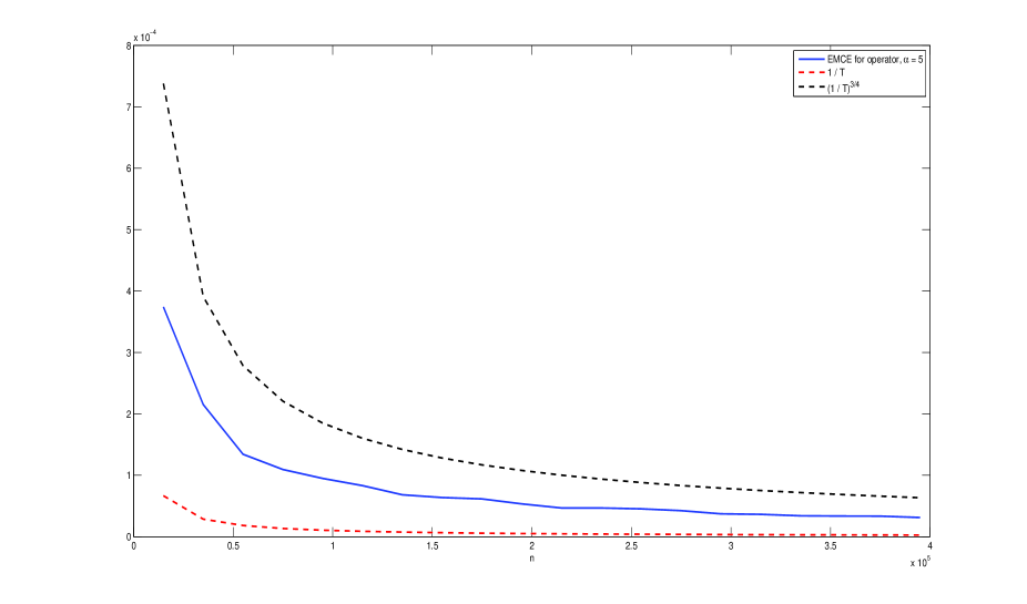
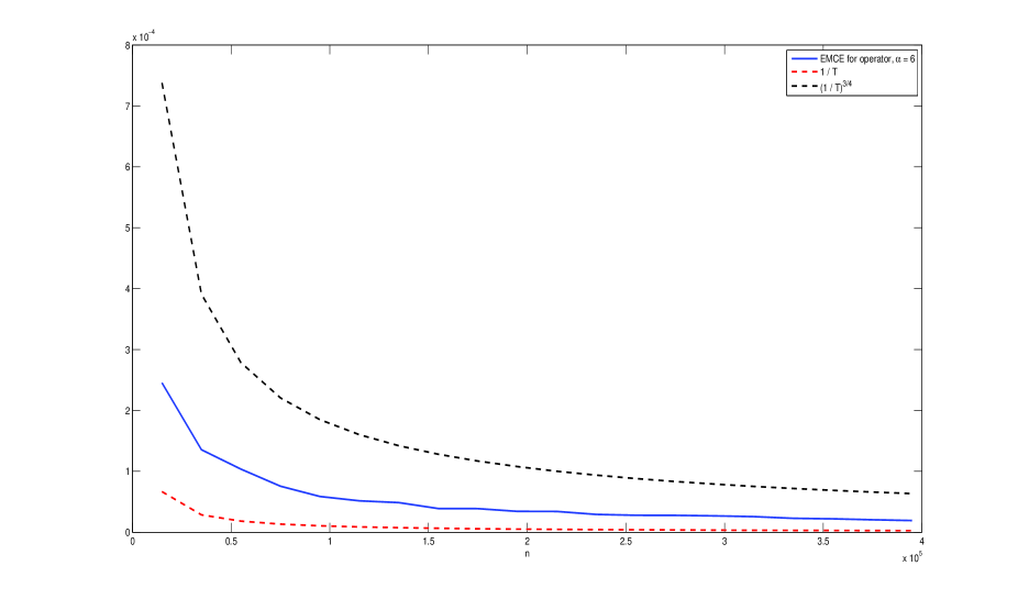
Figure 1: ${\rm EMSE}_{\widehat{\rho}_{k_{n}}}$ values (blue line), in (57)–(58), based on $N=700$ simulations, for $\gamma_{1}=0.4$ and $\gamma_{2}=9/20$, considering the sample sizes $\left\{n_{t}=15000+20000(t-1),\ t=1,\dots,20\right\}$ and the corresponding $k_{n,1}$ and $k_{n,2}$ values, for $\alpha_{1}=5$ (left-hand side) and $\alpha_{2}=6$ (right-hand side), against curves $(1/n_{t})^{3/4}$ (black dot line) and $1/n_{t}$ (red dot line).

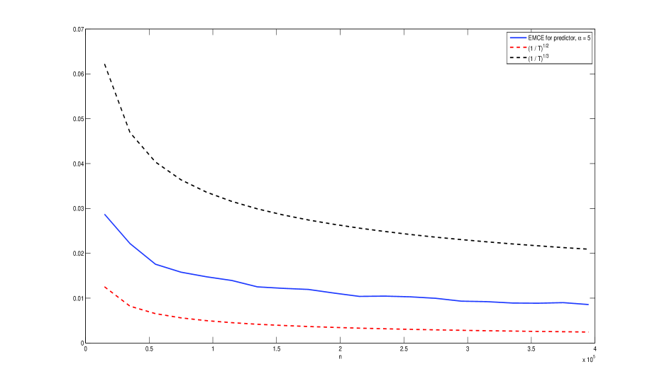
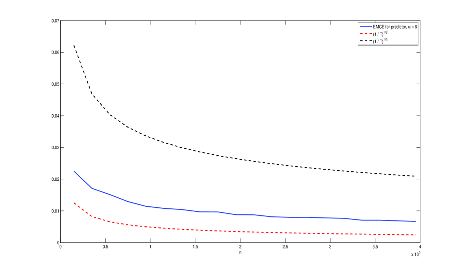
Figure 2: ${\rm UB(EMAE)}_{\widehat{X}_{n}^{k_{n}}}$ values (blue line), in (59), based on $N=700$ simulations, for $\gamma_{1}=0.4$ and $\gamma_{2}=9/20$, considering the sample sizes $\left\{n_{t}=15000+20000(t-1),\ t=1,\dots,20\right\}$ and the corresponding $k_{n,1}$ and $k_{n,2}$ values, for $\alpha_{1}=5$ (left-hand side) and $\alpha_{2}=6$ (right-hand side), against curves $(1/n_{t})^{1/2}$ (red dot line) and $(1/n_{t})^{1/3}$ (black dot line).

In this paper, a one–parameter model of $k_{n}$ is selected depending on parameter $\alpha$. In [Guillas, 2001, Example 2], in the same spirit, for an equivalent spectral class of operators $C$, a three–parameter model is established for $k_{n}$ to ensure convergence in quadratic mean in the space $\mathcal{L}(H)$ of the componentwise estimator of $\rho$ constructed from the known eigenvectors of $C$. The numerical results displayed in Table 1 and Figures 1–2 illustrate the fact that the proposed componentwise estimator $\widehat{\rho}_{k_{n}}$ presents a speed of convergence to $\rho,$ in quadratic mean in $S(H),$ faster than $n^{-1/3},$ which corresponds to the optimal case for the componentwise estimator of $\rho$ proposed in Guillas [2001], in the case of known eigenvectors of $C$; see, in particular, [Guillas, 2001, Theorem 1, Remark 2 and Example 2]. For larger values of the parameters $\gamma_{1}$ than $2.4,$ and $\alpha$ than $6$, a faster velocity of convergence of $\widehat{\rho}_{k_{n}}$ to $\rho,$ in quadratic mean in the space $S(H),$ will be obtained. However, larger sample sizes are required for larger values of $\alpha,$ in order to estimate a given number of coefficients of $\rho.$ A more detailed discussion about comparison of the rates of convergence of the ARH(1) plug–in predictors proposed in Antoniadis and Sapatinas [2003], Besse et al. [2000], Bosq [2000], Guillas [2001] can be found in the next section.

A comparative study

In this section, the performance of our approach is compared with those ones given in Antoniadis and Sapatinas [2003], Besse et al. [2000], Bosq [2000], Guillas [2001], including the case of unknown eigenvectors of $C.$ In the last case, our approach and the approaches presented in Bosq [2000], Guillas [2001] are implemented in terms of the empirical eigenvectors.

5.2.1 Theoretical–eigenvector–based componentwise estimators

Let us first compare the performance of our ARH(1) plug–in predictor, defined in (38), and the ones formulated in Bosq [2000], Guillas [2001], in terms of the theoretical eigenvectors $\left\{\phi_{j},\ j\geq 1\right\}$ of $C.$ Note that, in this first part of our comparative study, we consider the previous generated Gaussian ARH(1) process, with autocovariance and autocorrelation operators defined from equations (53) and (54), for different rates of convergence to zero of parameters $C_{j}$ and $\rho_{j}^{2},$ $j\geq 1,$ with both sequences being summable sequences. Since we restrict our attention to the Gaussian case, conditions A${}_{1},$ B₁ and C${}_{1},$ formulated in [Bosq, 2000, pp. 211–212] are satisfied by the generated ARH(1) process. Similarly, Conditions H₁–H₃ in [Guillas, 2001, p. 283] are satisfied as well.

In [Bosq, 2000, Section 8.2] the following estimator of $\rho$ is proposed

$$\widehat{\rho}_{n}(x) = \left(\Pi^{k_{n}}D_{n}\widehat{C}_{n}^{-1}\Pi^{k_{n}}\right)(x)=\displaystyle\sum_{l=1}^{k_{n}}\widehat{\rho}_{n,l}(x)\phi_{l},\quad x\in H,$$ (60)

$$\widehat{\rho}_{n,l}(x) = \frac{1}{n-1}\displaystyle\sum_{i=0}^{n-2}\displaystyle\sum_{j=1}^{k_{n}}\frac{1}{\widehat{C}_{n,j}}\langle\phi_{j},x\rangle_{H}X_{i,j}X_{i+1,l},$$ (61)

in the finite dimensional subspace

$$H_{k_{n}}={\rm span}\left(\phi_{1},\dots,\phi_{k_{n}}\right)$$

of $H,$ where $\Pi^{k_{n}}$ is the orthogonal projector over $H_{k_{n}},$ and, as before, $X_{i,j}=\left\langle X_{i},\phi_{j}\right\rangle_{H},$ for $j\geq 1.$

A modified estimator of $\rho$ is studied in [Guillas, 2001, Section 2], given by

$$\widehat{\rho}_{n,a}(x) = \left(\Pi^{k_{n}}D_{n}\widehat{C}_{n,a}^{-1}\Pi^{k_{n}}\right)(x)=\displaystyle\sum_{l=1}^{k_{n}}\widehat{\rho}_{n,a,l}(x)\phi_{l},\quad x\in H,$$ (62)

$$\widehat{\rho}_{n,a,l}(x) = \frac{1}{n-1}\displaystyle\sum_{i=1}^{n-1}\displaystyle\sum_{j=1}^{k_{n}}\frac{1}{\displaystyle\max\left(\widehat{C}_{n,j},\leavevmode\nobreak\ a_{n}\right)}\langle\phi_{j},x\rangle_{H}X_{i,j}X_{i+1,l}{\color[rgb]{0,1,0},}$$ (63)

where

$$\widehat{C}_{n,a}^{-1}(x)=\displaystyle\sum_{j=1}^{k_{n}}\frac{1}{\displaystyle\max\left(\widehat{C}_{n,j},\leavevmode\nobreak\ a_{n}\right)}\langle\phi_{j},x\rangle_{H}\phi_{j}\leavevmode\nobreak\ a.s.$$

Here, $\left\{a_{n},\ n\in\mathbb{N}\right\}$ is such that (see [Guillas, 2001, Theorem 1])

$$\alpha\frac{C_{k_{n}}^{\gamma}}{n^{\varepsilon}}\leq a_{n}\leq\beta\lambda_{k_{n}},\quad\alpha>0,\quad 0<\beta<1,\quad\varepsilon<1/2,\quad\gamma\geq 1.$$

Tables 2–3 display the truncated, for two different $k_{n}$ rules, empirical values of ${\rm E}\left\{\|\rho\left(X_{n-1}\right)-\widehat{\rho}_{k_{n}}(X_{n-1})\|_{H}\right\},$ based on $N=700$ generations of each one of the functional samples considered with sizes $n_{t}=15000+20000(t-1),$ $t=1,\dots,20,$ when

$$C_{j}=b_{C}j^{-\delta_{1}},\quad b_{C}>0,\quad\rho_{j}^{2}=b_{\rho}j^{-\delta_{2}},\quad b_{\rho}>0.$$

Specifically, $\widehat{\rho}_{k_{n}}$ is computed from equations (15)–(16) (see third column), $\widehat{\rho}_{k_{n}}=\widehat{\rho}_{n}$, with $\widehat{\rho}_{n}$ being given in equations (60)–(61) (see fourth column), and $\widehat{\rho}_{k_{n}}=\widehat{\rho}_{n,a}$, with $\widehat{\rho}_{n,a}$ being defined in (62)–(63) (see fifth column).

In Table 2, $\delta_{1}=2.4$ $\delta_{2}=1.1,$ and $k_{n}=\lceil n^{1/\alpha}\rceil,$ for $\alpha=6,$ according to our Assumption A3, which is also considered in [Bosq, 2000, p. 217] to ensure weak consistency of the proposed estimator of $\rho$. In Table 3, the same empirical values are displayed for $\delta_{1}=\frac{61}{60},$ $\delta_{2}=1.1,$ and $k_{n}$ is selected according to [Guillas, 2001, Example 2]. Thus, in Table 3,

$$k_{n}=\lceil n^{\frac{1-2\epsilon}{\delta_{1}(4+2\gamma)}}\rceil,\quad\gamma\geq 1,\ \epsilon<1/2.$$ (64)

In particular we have chosen $\gamma=2,$ and $\epsilon=0.04\delta_{1}.$ Note that, from [Guillas, 2001, Theorem 1 and Remark 1], for the choice made of $k_{n}$ in Table 3, convergence to $\rho,$ in quadratic mean in the space $\mathcal{L}(H),$ holds for $\widehat{\rho}_{n,a}$ given in (62)–(63).

Table 2: Truncated empirical values of ${\rm E}\|\rho\left(X_{n-1}\right)-\widehat{\rho}_{k_{n}}(X_{n-1})\|_{H},$ for $\widehat{\rho}_{k_{n}}$ given in equations (15)-(16) (third column), in equations (60)–(61) (fourth column), and in equations (62)–(63) (fifth column), based on $N=700$ simulations, for $\delta_{1}=2.4$ and $\delta_{2}=1.1,$ considering the sample sizes $\left\{n_{t}=15000+20000(t-1),\ t=1,\dots,20\right\}$ and the corresponding $k_{n}=\lceil n^{1/\alpha}\rceil$ values, for $\alpha=6$.

$n$	$k_{n}$	Our Approach	Bosq (2000)	Guillas (2001)
$n_{1}=15000$	$4$	$2.25\left(10\right)^{-2}$	$2.57\left(10\right)^{-2}$	$2.36\left(10\right)^{-2}$
$n_{2}=35000$	$5$	$1.71\left(10\right)^{-2}$	$1.72\left(10\right)^{-2}$	$1.84\left(10\right)^{-2}$
$n_{3}=55000$	$6$	$1.51\left(10\right)^{-2}$	$1.65\left(10\right)^{-2}$	$1.53\left(10\right)^{-2}$
$n_{4}=75000$	$6$	$1.29\left(10\right)^{-2}$	$1.46\left(10\right)^{-2}$	$1.37\left(10\right)^{-2}$
$n_{5}=95000$	$6$	$1.14\left(10\right)^{-2}$	$1.20\left(10\right)^{-2}$	$1.16\left(10\right)^{-2}$
$n_{6}=115000$	$6$	$1.07\left(10\right)^{-2}$	$1.10\left(10\right)^{-2}$	$1.11\left(10\right)^{-2}$
$n_{7}=135000$	$7$	$1.04\left(10\right)^{-2}$	$1.06\left(10\right)^{-2}$	$1.07\left(10\right)^{-2}$
$n_{8}=155000$	$7$	$9.66\left(10\right)^{-3}$	$9.91\left(10\right)^{-3}$	$1.01\left(10\right)^{-2}$
$n_{9}=175000$	$7$	$9.65\left(10\right)^{-3}$	$9.79\left(10\right)^{-3}$	$9.68\left(10\right)^{-3}$
$n_{10}=195000$	$7$	$8.79\left(10\right)^{-3}$	$9.12\left(10\right)^{-3}$	$8.93\left(10\right)^{-3}$
$n_{11}=215000$	$7$	$8.74\left(10\right)^{-3}$	$8.79\left(10\right)^{-3}$	$8.83\left(10\right)^{-3}$
$n_{12}=235000$	$7$	$8.12\left(10\right)^{-3}$	$8.69\left(10\right)^{-3}$	$8.75\left(10\right)^{-3}$
$n_{13}=255000$	$7$	$7.95\left(10\right)^{-3}$	$8.53\left(10\right)^{-3}$	$8.73\left(10\right)^{-3}$
$n_{14}=275000$	$8$	$7.94\left(10\right)^{-3}$	$8.52\left(10\right)^{-3}$	$8.58\left(10\right)^{-3}$
$n_{15}=295000$	$8$	$7.76\left(10\right)^{-3}$	$8.49\left(10\right)^{-3}$	$8.36\left(10\right)^{-3}$
$n_{16}=315000$	$8$	$7.64\left(10\right)^{-3}$	$7.88\left(10\right)^{-3}$	$8.13\left(10\right)^{-3}$
$n_{17}=335000$	$8$	$7.04\left(10\right)^{-3}$	$7.24\left(10\right)^{-3}$	$7.59\left(10\right)^{-3}$
$n_{18}=355000$	$8$	$7.04\left(10\right)^{-3}$	$7.23\left(10\right)^{-3}$	$6.92\left(10\right)^{-3}$
$n_{19}=375000$	$8$	$6.84\left(10\right)^{-3}$	$6.89\left(10\right)^{-3}$	$6.90\left(10\right)^{-3}$
$n_{20}=395000$	$8$	$6.65\left(10\right)^{-3}$	$6.67\left(10\right)^{-3}$	$6.85\left(10\right)^{-3}$

Table 3: Truncated empirical values of ${\rm E}\|\rho\left(X_{n-1}\right)-\widehat{\rho}_{k_{n}}(X_{n-1})\|_{H},$ for $\widehat{\rho}_{k_{n}}$ given in equations (15)–(16) (third column), in equations (60)–(61) (fourth column), and in equations (62)–(63) (fifth column), based on $N=700$ simulations, for $\delta_{1}=\frac{61}{60}$ and $\delta_{2}=1.1,$ considering the sample sizes $\left\{n_{t}=15000+20000(t-1),\ t=1,\dots,20\right\}$ and the corresponding $k_{n}$ given in (64).

$n$	$k_{n}$	Our Approach	Bosq (2000)	Guillas (2001)
$n_{1}=15000$	$2$	$9.91\left(10\right)^{-3}$	$1.39\left(10\right)^{-2}$	$1.26\left(10\right)^{-2}$
$n_{2}=35000$	$3$	$8.78\left(10\right)^{-3}$	$1.34\left(10\right)^{-2}$	$1.24\left(10\right)^{-2}$
$n_{3}=55000$	$3$	$7.89\left(10\right)^{-3}$	$1.15\left(10\right)^{-2}$	$1.14\left(10\right)^{-2}$
$n_{4}=75000$	$3$	$6.49\left(10\right)^{-3}$	$1.01\left(10\right)^{-2}$	$8.58\left(10\right)^{-3}$
$n_{5}=95000$	$3$	$6.36\left(10\right)^{-3}$	$9.09\left(10\right)^{-3}$	$8.29\left(10\right)^{-3}$
$n_{6}=115000$	$3$	$6.14\left(10\right)^{-3}$	$7.65\left(10\right)^{-3}$	$7.26\left(10\right)^{-3}$
$n_{7}=135000$	$3$	$5.91\left(10\right)^{-3}$	$7.03\left(10\right)^{-3}$	$6.69\left(10\right)^{-3}$
$n_{8}=155000$	$3$	$5.73\left(10\right)^{-3}$	$6.77\left(10\right)^{-3}$	$6.54\left(10\right)^{-3}$
$n_{9}=175000$	$3$	$5.44\left(10\right)^{-3}$	$6.74\left(10\right)^{-3}$	$6.16\left(10\right)^{-3}$
$n_{10}=195000$	$3$	$5.10\left(10\right)^{-3}$	$6.69\left(10\right)^{-3}$	$5.97\left(10\right)^{-3}$
$n_{11}=215000$	$4$	$5.01\left(10\right)^{-3}$	$6.48\left(10\right)^{-3}$	$5.94\left(10\right)^{-3}$
$n_{12}=235000$	$4$	$4.85\left(10\right)^{-3}$	$6.45\left(10\right)^{-3}$	$5.83\left(10\right)^{-3}$
$n_{13}=255000$	$4$	$4.17\left(10\right)^{-3}$	$6.17\left(10\right)^{-3}$	$5.68\left(10\right)^{-3}$
$n_{14}=275000$	$4$	$4.64\left(10\right)^{-3}$	$5.99\left(10\right)^{-3}$	$5.60\left(10\right)^{-3}$
$n_{15}=295000$	$4$	$4.55\left(10\right)^{-3}$	$5.94\left(10\right)^{-3}$	$5.58\left(10\right)^{-3}$
$n_{16}=315000$	$4$	$4.48\left(10\right)^{-3}$	$5.69\left(10\right)^{-3}$	$5.50\left(10\right)^{-3}$
$n_{17}=335000$	$4$	$4.38\left(10\right)^{-3}$	$5.58\left(10\right)^{-3}$	$5.44\left(10\right)^{-3}$
$n_{18}=355000$	$4$	$4.16\left(10\right)^{-3}$	$5.45\left(10\right)^{-3}$	$5.42\left(10\right)^{-3}$
$n_{19}=375000$	$4$	$3.91\left(10\right)^{-3}$	$5.34\left(10\right)^{-3}$	$5.32\left(10\right)^{-3}$
$n_{20}=395000$	$4$	$3.86\left(10\right)^{-3}$	$5.29\left(10\right)^{-3}$	$5.26\left(10\right)^{-3}$

One can observe in Table 2 a similar performance of the three methods compared with the truncation order kn satisfying Assumption A3, with slightly worse results being obtained from the estimator defined in (62)–(63), specially, for the sample size $n_{8}=155000.$ Furthermore, in Table 3, a better performance of our approach is observed for the smallest sample sizes (from $n_{1}=15000$ until $n_{4}=75000$). For the remaining largest sample sizes, only slight differences are observed, with, again, a better performance of our approach, very close to the other two approaches presented in Bosq [2000], Guillas [2001].

5.2.2 Empirical–eigenvector–based componentwise estimators

In this section, we address the case where $\left\{\phi_{j},\ j\geq 1\right\}$ are unknown, as is often the case in practice. Specifically, for a given sample size $n$, let $\left\{\phi_{n,j},\ j\geq 1\right\}$ be the empirical counterpart of the theoretical eigenvectors $\left\{\phi_{j},\ j\geq 1\right\}$, satisfying, for every $j\geq 1$,

$$C_{n}\left(\phi_{n,j}\right)=\frac{1}{n}\displaystyle\sum_{i=0}^{n-1}\langle X_{i},\phi_{n,j}\rangle_{H}X_{i}=C_{n,j}\phi_{n,j},$$

where $\left\{C_{n,j},\ j\geq 1\right\}$ denotes the system of eigenvalues associated with the system of empirical eigenvectors $\left\{\phi_{n,j},\ j\geq 1\right\}$. We then consider the following estimators for comparison purposes

$$\widetilde{\rho}_{n,j} = \frac{\frac{1}{n-1}\displaystyle\sum_{i=0}^{n-2}\widetilde{X}_{i,j}\widetilde{X}_{i+1,j}}{\frac{1}{n}\displaystyle\sum_{i=0}^{n-1}\left(\widetilde{X}_{i,j}\right)^{2}},\quad\widetilde{\rho}_{k_{n}}=\sum_{j=1}^{k_{n}}\widetilde{\rho}_{n,j}\phi_{n,j}\otimes\phi_{n,j},$$ (65)

$$\widetilde{\rho}_{n}(x) = \left(\widetilde{\Pi}^{k_{n}}D_{n}C_{n}^{-1}\widetilde{\Pi}^{k_{n}}\right)(x)=\displaystyle\sum_{l=1}^{k_{n}}\widetilde{\rho}_{n,l}(x)\phi_{n,l},\quad x\in H,$$

$$\widetilde{\rho}_{n,l}(x) = \frac{1}{n-1}\displaystyle\sum_{i=0}^{n-2}\displaystyle\sum_{j=1}^{k_{n}}\frac{1}{C_{n,j}}\langle\phi_{n,j},x\rangle_{H}\widetilde{X}_{i,j}\widetilde{X}_{i+1,l},$$ (66)

$$\widetilde{\rho}_{n,a}(x) = \left(\widetilde{\Pi}^{k_{n}}D_{n}C_{n,a}^{-1}\widetilde{\Pi}^{k_{n}}\right)(x)=\displaystyle\sum_{l=1}^{k_{n}}\widetilde{\rho}_{n,a,l}(x)\phi_{n,l},\quad x\in H,$$

$$\widetilde{\rho}_{n,a,l}(x) = \frac{1}{n-1}\displaystyle\sum_{i=0}^{n-2}\displaystyle\sum_{j=1}^{k_{n}}\frac{1}{\displaystyle\max\left(C_{n,j},a_{n}\right)}\langle\phi_{n,j},x\rangle_{H}\widetilde{X}_{i,j}\widetilde{X}_{i+1,l,}$$ (67)

where, for $i\in\mathbb{Z},$ and $j\geq 1,$ $\widetilde{X}_{i,j}=\left\langle X_{i},\phi_{n,j}\right\rangle_{H},$ $\widetilde{\Pi}^{k_{n}}$ denotes the orthogonal projector into the space

$$\widetilde{H}_{k_{n}}={\rm span}\left(\phi_{n,1},\dots,\phi_{n,k_{n}}\right).$$

The Gaussian ARH(1) process is generated under Assumptions A1–A2, as well as $C_{1}^{\prime}$ in [Bosq, 2000, p. 218]. Note that conditions $A_{1}$ and $B_{1}^{\prime}$ in Bosq [2000] already hold. Moreover, as given in [Bosq, 2000, Theorem 8.8 and Example 8.6], for

$$C_{j}=b_{C}j^{-\delta_{1}},\quad b_{C}>0,\quad\delta_{1}>0,$$

with, in particular, $\delta_{1}=2.4,$ and for

$$\rho_{j}=b_{\rho}j^{-\delta_{2}},\quad b_{\rho}>0,$$

with $\delta_{2}=1.1,$, the estimator $\widetilde{\rho}_{n}$ converges almost surely to $\rho$ under the condition

$$\frac{nC_{kn}^{2}}{\ln(n)\left(\displaystyle\sum_{j=1}^{k_{n}}b_{j}\right)^{2}}\longrightarrow\infty,$$

where

$$b_{1}=2\sqrt{2}\left(C_{1}-C_{2}\right)^{-1},\quad b_{j}=2\sqrt{2}\max\left\{(C_{j-1}-C_{j})^{-1},(C_{j}-C_{j+1})^{-1}\right\},\leavevmode\nobreak\ j\geq 2.$$

In Table 4, $k_{n}=\lceil\ln(n)\rceil$ has been tested; see [Bosq, 2000, Example 8.6].

Table 4: Truncated empirical values of ${\rm E}\left\{\left\|\rho\left(X_{n-1}\right)-\widetilde{\rho}_{k_{n}}\left(X_{n-1}\right)\right\|_{H}\right\}$, for $\widetilde{\rho}_{k_{n}}=\widetilde{\rho}_{k_{n}}$ given in equation (65) (third column), $\widetilde{\rho}_{k_{n}}=\widetilde{\rho}_{n}$ defined in equation (66) (fourth column) and $\widetilde{\rho}_{k_{n}}=\widetilde{\rho}_{n,a}$ defined in equation (67) (fifth column), based on $N=700$ simulations, for $\delta_{1}=2.4$ and $\delta_{2}=1.1,$ considering the sample sizes $\left\{n_{t}=15000+20000(t-1),\ t=1,\dots,20\right\}$ and $k_{n}=\lceil\ln(n)\rceil$.

$n$	$k_{n}$	Our approach	Bosq (2000)	Guillas (2001)
$n_{1}=15000$	$9$	$8.42\left(10\right)^{-2}$	$1.061$	$1.035$
$n_{2}=35000$	$10$	$5.51\left(10\right)^{-2}$	$1.019$	$1.005$
$n_{3}=55000$	$10$	$4.75\left(10\right)^{-2}$	$1.017$	$0.999$
$n_{4}=75000$	$11$	$4.43\left(10\right)^{-2}$	$1.015$	$0.995$
$n_{5}=95000$	$11$	$3.68\left(10\right)^{-2}$	$1.013$	$0.988$
$n_{6}=115000$	$11$	$3.51\left(10\right)^{-2}$	$1.011$	$0.963$
$n_{7}=135000$	$11$	$3.23\left(10\right)^{-2}$	$1.008$	$0.925$
$n_{8}=155000$	$11$	$2.95\left(10\right)^{-2}$	$1.007$	$0.912$
$n_{9}=175000$	$12$	$2.94\left(10\right)^{-2}$	$1.006$	$0.911$
$n_{10}=195000$	$12$	$2.80\left(10\right)^{-2}$	$0.995$	$0.891$
$n_{11}=215000$	$12$	$2.71\left(10\right)^{-2}$	$0.902$	$0.862$
$n_{12}=235000$	$12$	$2.59\left(10\right)^{-2}$	$0.890$	$0.820$
$n_{13}=255000$	$12$	$2.58\left(10\right)^{-2}$	$0.878$	$0.800$
$n_{14}=275000$	$12$	$2.35\left(10\right)^{-2}$	$0.872$	$0.783$
$n_{15}=295000$	$12$	$2.28\left(10\right)^{-2}$	$0.860$	$0.778$
$n_{16}=315000$	$12$	$2.27\left(10\right)^{-2}$	$0.842$	$0.747$
$n_{17}=335000$	$12$	$2.16\left(10\right)^{-2}$	$0.822$	$0.714$
$n_{18}=355000$	$12$	$2.14\left(10\right)^{-2}$	$0.800$	$0.707$
$n_{19}=375000$	$12$	$2.09\left(10\right)^{-2}$	$0.778$	$0.687$
$n_{20}=395000$	$12$	$2.06\left(10\right)^{-2}$	$0.769$	$0.662$

A better performance of our estimator (65) in comparison with estimator (66), formulated in Bosq [2000], and estimator (67), formulated in [Guillas, 2001, Example 4 and Remark 4], is observed in Table 4. Note that, in particular, in [Guillas, 2001, Example 4 and Remark 4], smaller values of $k_{n}$ than $\ln(n)$ are required for a given sample size $n,$ to ensure convergence in quadratic mean, and, in particular, weak–consistency. However, considering a smaller discretization step size $\Delta t=0.015$ than in Table 4, where $\Delta t=0.08$, and for $k_{n}=\lceil n^{1/6}\rceil,$ (i.e., $\alpha=6$), we obtain in Table 5, for the same parameter values $\delta_{1}=2.4$ and $\delta_{2}=1.1,$ better results than in Table 4, since a smaller number of coefficients of $\rho$ (parameters) to be estimated is considered in Table 5, from a richer sample information (coming from the smaller discretization step size considered). One can also observe in Table 5 a similar performance of the three approaches studied. In Table 6, the value $k_{n}=\lceil e^{\prime}n^{1/\left(8\delta_{1}+2\right)}\rceil$, with $e^{\prime}=\frac{17}{10}$ proposed in [Guillas, 2001, Example 4 and Remark 4] is considered to compute the truncated empirical values of ${\rm E}\left\{\|\rho(X_{n-1})-\widetilde{\rho}_{k_{n}}(X_{n-1})\|_{H}\right\},$ for $\widetilde{\rho}_{k_{n}}$ defined in equation (65) (third column), for $\widetilde{\rho}_{k_{n}}=\widetilde{\rho}_{n}$ given in equation (66) (fourth column), and for $\widetilde{\rho}_{k_{n}}=\widetilde{\rho}_{n,a}$ in equation (67) (fifth column). A similar performance of the three approaches is observed, with the exception of $n_{20}=395000,$ where the approach presented in Guillas [2001] displays a slightly better performance

Table 5: Truncated empirical values of ${\rm E}\left\{\left\|\rho\left(X_{n-1}\right)-\widetilde{\rho}_{k_{n}}\left(X_{n-1}\right)\right\|_{H}\right\}$, for $\widetilde{\rho}_{k_{n}}$ defined in equation (65) (third column), for $\widetilde{\rho}_{k_{n}}=\widetilde{\rho}_{n}$ given in equation (66) (fourth column), and for $\widetilde{\rho}_{k_{n}}=\widetilde{\rho}_{n,a}$ in equation (67) (fifth column), based on $N=200$ (due to high-dimensionality) simulations, for $\delta_{1}=2.4$ and $\delta_{2}=1.1,$ considering the sample sizes $\left\{n_{t}=15000+20000(t-1),\ t=1,\dots,20\right\}$ and $k_{n}=\lceil n^{1/6}\rceil.$

$n$	$k_{n}$	Our approach	Bosq (2000)	Guillas (2001)
$n_{1}=15000$	$4$	$9.88\left(10\right)^{-2}$	$9.25\left(10\right)^{-2}$	$0.106$
$n_{2}=35000$	$5$	$9.52\left(10\right)^{-2}$	$9.07\left(10\right)^{-2}$	$9.86\left(10\right)^{-2}$
$n_{3}=55000$	$6$	$9.12\left(10\right)^{-2}$	$8.92\left(10\right)^{-2}$	$9.39\left(10\right)^{-2}$
$n_{4}=75000$	$6$	$8.48\left(10\right)^{-2}$	$8.64\left(10\right)^{-2}$	$8.98\left(10\right)^{-2}$
$n_{5}=95000$	$6$	$7.61\left(10\right)^{-2}$	$8.30\left(10\right)^{-2}$	$8.46\left(10\right)^{-2}$
$n_{6}=115000$	$6$	$7.05\left(10\right)^{-2}$	$7.96\left(10\right)^{-2}$	$8.04\left(10\right)^{-2}$
$n_{7}=135000$	$7$	$6.99\left(10\right)^{-2}$	$7.84\left(10\right)^{-2}$	$7.82\left(10\right)^{-2}$
$n_{8}=155000$	$7$	$6.70\left(10\right)^{-2}$	$7.45\left(10\right)^{-2}$	$7.40\left(10\right)^{-2}$
$n_{9}=175000$	$7$	$6.49\left(10\right)^{-2}$	$7.03\left(10\right)^{-2}$	$7.07\left(10\right)^{-2}$
$n_{10}=195000$	$7$	$5.88\left(10\right)^{-2}$	$6.74\left(10\right)^{-2}$	$6.80\left(10\right)^{-2}$
$n_{11}=215000$	$7$	$5.63\left(10\right)^{-2}$	$6.46\left(10\right)^{-2}$	$6.57\left(10\right)^{-2}$
$n_{12}=235000$	$7$	$5.30\left(10\right)^{-2}$	$6.28\left(10\right)^{-2}$	$6.37\left(10\right)^{-2}$
$n_{13}=255000$	$7$	$5.05\left(10\right)^{-2}$	$6.19\left(10\right)^{-2}$	$6.24\left(10\right)^{-2}$
$n_{14}=275000$	$8$	$4.88\left(10\right)^{-2}$	$5.99\left(10\right)^{-2}$	$6.15\left(10\right)^{-2}$
$n_{15}=295000$	$8$	$4.58\left(10\right)^{-2}$	$5.74\left(10\right)^{-2}$	$6.04\left(10\right)^{-2}$
$n_{16}=315000$	$8$	$4.24\left(10\right)^{-2}$	$5.52\left(10\right)^{-2}$	$5.93\left(10\right)^{-2}$
$n_{17}=335000$	$8$	$3.86\left(10\right)^{-2}$	$5.24\left(10\right)^{-2}$	$5.70\left(10\right)^{-2}$
$n_{18}=355000$	$8$	$3.70\left(10\right)^{-2}$	$5.02\left(10\right)^{-2}$	$5.53\left(10\right)^{-2}$
$n_{19}=375000$	$8$	$3.55\left(10\right)^{-2}$	$4.88\left(10\right)^{-2}$	$5.36\left(10\right)^{-2}$
$n_{20}=395000$	$8$	$3.46\left(10\right)^{-2}$	$4.70\left(10\right)^{-2}$	$5.23\left(10\right)^{-2}$

Table 6: Truncated empirical values of ${\rm E}\left\{\left\|\rho\left(X_{n-1}\right)-\widetilde{\rho}_{k_{n}}\left(X_{n-1}\right)\right\|_{H}\right\}$, for $\widetilde{\rho}_{k_{n}}$ defined in equation (65) (third column), for $\widetilde{\rho}_{k_{n}}=\widetilde{\rho}_{n}$ given in equation (66) (fourth column), and for $\widetilde{\rho}_{k_{n}}=\widetilde{\rho}_{n,a}$ in equation (67) (fifth column), based on $N=200$ (due to high-dimensionality) simulations, for $\delta_{1}=2.4$ and $\delta_{2}=1.1,$ considering the sample sizes $\left\{n_{t}=15000+20000(t-1),\ t=1,\dots,20\right\}$ and $k_{n}=\lceil e^{\prime}n^{1/\left(8\delta_{1}+2\right)}\rceil,\leavevmode\nobreak\ e^{\prime}=\frac{17}{10}.$

$n$	$k_{n}$	Our approach	Bosq (2000)	Guillas (2001)
$n_{1}=15000$	$2$	$6.78\left(10\right)^{-2}$	$8.77\left(10\right)^{-2}$	$6.64\left(10\right)^{-2}$
$n_{2}=35000$	$2$	$6.72\left(10\right)^{-2}$	$8.61\left(10\right)^{-2}$	$6.30\left(10\right)^{-2}$
$n_{3}=55000$	$2$	$6.46\left(10\right)^{-2}$	$8.48\left(10\right)^{-2}$	$6.17\left(10\right)^{-2}$
$n_{4}=75000$	$2$	$6.24\left(10\right)^{-2}$	$8.20\left(10\right)^{-2}$	$5.76\left(10\right)^{-2}$
$n_{5}=95000$	$2$	$5.42\left(10\right)^{-2}$	$7.84\left(10\right)^{-2}$	$5.03\left(10\right)^{-2}$
$n_{6}=115000$	$2$	$4.84\left(10\right)^{-2}$	$7.34\left(10\right)^{-2}$	$4.56\left(10\right)^{-2}$
$n_{7}=135000$	$2$	$4.27\left(10\right)^{-2}$	$6.95\left(10\right)^{-2}$	$3.94\left(10\right)^{-2}$
$n_{8}=155000$	$2$	$3.64\left(10\right)^{-2}$	$6.60\left(10\right)^{-2}$	$3.65\left(10\right)^{-2}$
$n_{9}=175000$	$3$	$3.51\left(10\right)^{-2}$	$6.52\left(10\right)^{-2}$	$3.42\left(10\right)^{-2}$
$n_{10}=195000$	$3$	$3.38\left(10\right)^{-2}$	$6.16\left(10\right)^{-2}$	$3.24\left(10\right)^{-2}$
$n_{11}=215000$	$3$	$3.16\left(10\right)^{-2}$	$5.78\left(10\right)^{-2}$	$2.85\left(10\right)^{-2}$
$n_{12}=235000$	$3$	$2.98\left(10\right)^{-2}$	$5.53\left(10\right)^{-2}$	$2.60\left(10\right)^{-2}$
$n_{13}=255000$	$3$	$2.83\left(10\right)^{-2}$	$5.15\left(10\right)^{-2}$	$2.34\left(10\right)^{-2}$
$n_{14}=275000$	$3$	$2.50\left(10\right)^{-2}$	$4.85\left(10\right)^{-2}$	$2.05\left(10\right)^{-2}$
$n_{15}=295000$	$3$	$2.23\left(10\right)^{-2}$	$4.46\left(10\right)^{-2}$	$1.83\left(10\right)^{-2}$
$n_{16}=315000$	$3$	$2.15\left(10\right)^{-2}$	$4.30\left(10\right)^{-2}$	$1.58\left(10\right)^{-2}$
$n_{17}=335000$	$3$	$2.06\left(10\right)^{-2}$	$4.14\left(10\right)^{-2}$	$1.40\left(10\right)^{-2}$
$n_{18}=355000$	$3$	$1.98\left(10\right)^{-2}$	$3.95\left(10\right)^{-2}$	$1.24\left(10\right)^{-2}$
$n_{19}=375000$	$3$	$1.89\left(10\right)^{-2}$	$3.77\left(10\right)^{-2}$	$1.05\left(10\right)^{-2}$
$n_{20}=395000$	$3$	$1.82\left(10\right)^{-2}$	$3.70\left(10\right)^{-2}$	$9.93\left(10\right)^{-3}$

5.2.3 Kernel–based nonparametric and penalized estimation

In practice, curves are observed in discrete times, and should be approximated by smooth functions. In Besse et al. [2000], the following optimization problem is considered:

$$\widehat{X}_{i}=argmin\left\|L\widehat{X}_{i}\right\|_{L^{2}}^{2},\leavevmode\nobreak\ \widehat{X}_{i}(t_{j})=X_{i}(t_{j}),\quad j=1,\dots,p,\leavevmode\nobreak\ i=0,\dots,n-1,$$ (68)

where $L$ is a linear differential operator of order $d.$ Our interpolation is computed by Matlab smoothingspline method. Non-linear kernel regression is then considered, in terms of the smoothed functional data, solution to (68), as follows:

$$\widehat{X}_{n}^{h_{n}} = \widehat{\rho}_{h_{n}}(X_{n-1}),\quad\widehat{\rho}_{h_{n}}(x)=\frac{\displaystyle\sum_{i=0}^{n-2}\widehat{X}_{i+1}K\left(\frac{\left\|\widehat{X}_{i}-x\right\|_{L^{2}}^{2}}{h_{n}}\right)}{\displaystyle\sum_{i=0}^{n-2}K\left(\frac{\left\|\widehat{X}_{i}-x\right\|_{L^{2}}^{2}}{h_{n}}\right)},$$

where $K$ is the usual Gaussian kernel, and

$$\left\|\widehat{X}_{i}-x\right\|_{L^{2}}^{2}=\int(\widehat{X}_{i}(t)-x(t))^{2}dt,\quad i=0,\dots,n-2.$$

Alternatively, in Besse et al. [2000], prediction, in the context of functional autoregressive processes (FAR(1) processes), under the linear assumption on $\rho,$ which is considered to be a compact operator, with $\|\rho\|<1,$ is also studied, from smooth data $\widehat{X}_{1},\dots,\widehat{X}_{n},$ solving the optimization problem

$$\min_{\widehat{X}_{i}\in H_{q}}\frac{1}{n}\displaystyle\sum_{i=0}^{n-1}\left(\frac{1}{p}\displaystyle\sum_{j=1}^{p}\left(X_{i}(t_{j})-\widehat{X}_{i}^{q,l}(t_{j})\right)^{2}+l\left\|D^{2}\widehat{X}_{i}^{q,l}\right\|_{L^{2}}^{2}\right),$$ (69)

where $l$ is the smoothing parameter, $H_{q}$ is the $q$–dimensional functional subspace spanned by the leading eigenvectors of the autocovariance operator $C$ associated with its largest eigenvalues. Thus, smoothness and rank constraint are considered in the computation of the solution to the optimization problem (69). Such a solution is obtained by means of functional PCA.

The following regularized empirical estimators of $C$ and $D$ are then considered, with inversion of $C$ in the subspace $H_{q}$:

$$\widehat{C}_{q,l}=\frac{1}{n}\sum_{i=0}^{n-1}\widehat{X}_{i}\otimes\widehat{X}_{i},\quad\widehat{D}_{q,l}=\frac{1}{n-1}\sum_{i=0}^{n-2}\widehat{X}_{i}\otimes\widehat{X}_{i+1}.$$

Thus, the regularized estimator of $\rho$ is given by

$$\widehat{\rho}_{q,l}=\widehat{D}_{q,l}\widehat{C}_{q,l}^{-1},$$

and the predictor

$$\widehat{X}_{n}^{q,l}=\widehat{\rho}_{q,l}X_{n-1}.$$

Due to computational cost limitations, in Table 7, the following statistics are evaluated to compare the performance of the two above-referred prediction methodologies:

$$EMAE_{\widehat{X}_{n}}^{h_{n}}=\frac{1}{p}\displaystyle\sum_{j=1}^{p}\left(X_{n}(t_{j})-\widehat{X}_{n}^{h_{n}}(t_{j})\right)^{2},$$ (70)

$$EMAE_{\widehat{X}_{n}}^{q,l}=\frac{1}{p}\displaystyle\sum_{j=1}^{p}\left(X_{n}(t_{j})-\widehat{X}_{n}^{q,l}(t_{j})\right)^{2}.$$ (71)

Table 7: $EMAE_{\widehat{X}_{n}}^{h_{n,i}},$ $i=1,2,$ and $EMAE_{\widehat{X}_{n}}^{q,l}$ values (see (70) and (71), respectively), with $q=7$, based on $N=200$ simulations, for $\delta_{1}=2.4$ and $\delta_{2}=1.1,$ considering now the sample sizes $\left\{n_{t}=750+500(t-1),\ t=1,\dots,13\right\}$ $h_{n,1}=0.1$ and $h_{n,2}=0.3$.

$n$	$EMAE_{\widehat{X}_{n}}^{h_{n,1}}$	$EMAE_{\widehat{X}_{n}}^{h_{n,2}}$	$EMAE_{\widehat{X}_{n}}^{q,l}$
$n_{1}=750$	$8.57\left(10\right)^{-2}$	$8.85\left(10\right)^{-2}$	$8.99\left(10\right)^{-2}$
$n_{2}=1250$	$7.67\left(10\right)^{-2}$	$8.43\left(10\right)^{-2}$	$8.69\left(10\right)^{-2}$
$n_{3}=1750$	$7.15\left(10\right)^{-2}$	$7.12\left(10\right)^{-2}$	$8.05\left(10\right)^{-2}$
$n_{4}=2250$	$7.09\left(10\right)^{-2}$	$6.87\left(10\right)^{-2}$	$7.59\left(10\right)^{-2}$
$n_{5}=2750$	$6.87\left(10\right)^{-2}$	$6.67\left(10\right)^{-2}$	$7.31\left(10\right)^{-2}$
$n_{6}=3250$	$6.52\left(10\right)^{-2}$	$5.92\left(10\right)^{-2}$	$7.28\left(10\right)^{-2}$
$n_{7}=3750$	$6.20\left(10\right)^{-2}$	$5.56\left(10\right)^{-2}$	$7.13\left(10\right)^{-2}$
$n_{8}=4250$	$6.06\left(10\right)^{-2}$	$5.32\left(10\right)^{-2}$	$7.06\left(10\right)^{-2}$
$n_{9}=4750$	$5.67\left(10\right)^{-2}$	$5.25\left(10\right)^{-2}$	$6.47\left(10\right)^{-2}$
$n_{10}=5250$	$5.24\left(10\right)^{-2}$	$5.12\left(10\right)^{-2}$	$6.08\left(10\right)^{-2}$
$n_{11}=5750$	$5.01\left(10\right)^{-2}$	$4.82\left(10\right)^{-2}$	$5.75\left(10\right)^{-2}$
$n_{12}=6250$	$4.90\left(10\right)^{-2}$	$4.49\left(10\right)^{-2}$	$5.33\left(10\right)^{-2}$
$n_{13}=6750$	$4.87\left(10\right)^{-2}$	$3.87\left(10\right)^{-2}$	$4.97\left(10\right)^{-2}$

It can be observed a similar performance of the kernel–based and penalized FAR(1) predictors, from smooth functional data, which is also comparable, considering one realization, to the performance obtained in Table 6, from the empirical eigenvectors.

5.2.4 Wavelet–based prediction for ARH(1) processes

The approach presented in Antoniadis and Sapatinas [2003] is now studied. Specifically, wavelet-based regularization is applied to obtain smooth estimates of the sample paths. The projection onto the space $V_{J},$ generated by translations of the scaling function $\phi_{Jk},\ k=0,\dots,2^{J}-1,$ at level $J,$ associated with a multiresolution analysis of $H,$ is first considered. For a given primary resolution level $j_{0}$, with $j_{0}<J,$ the following wavelet decomposition at $J-j_{0}$ resolution levels can be computed for any projected curve $\Phi_{V_{J}}X_{i},$ in the space $V_{J},$ for $i=0,\dots,n-1:$

$$\Phi_{V_{J}}X_{i}=\displaystyle\sum_{k=0}^{2^{j_{0}}-1}c_{j_{0}k}^{i}\phi_{j_{0}k}+\displaystyle\sum_{j=j_{0}}^{J-1}\displaystyle\sum_{k=0}^{2^{j}-1}d_{jk}^{i}\psi_{jk},$$

$$c_{j_{0}k}^{i}=\langle\Phi_{V_{J}}X_{i},\phi_{j_{0}k}\rangle_{H},\leavevmode\nobreak\ d_{jk}^{i}=\langle\Phi_{V_{J}}X_{i},\psi_{jk}\rangle_{H}.$$

For $i=0,\dots,n-1,$ the following variational problem is solved to obtain the smooth estimate of the curve $X_{i}:$

$$\inf_{f^{i}\in H}\left\{\left\|\Phi_{V_{J}}X_{i}-f^{i}\right\|_{L^{2}}^{2}+\lambda\left\|\Phi_{V_{j_{0}}^{\bot}}f\right\|^{2};\leavevmode\nobreak\ f\in H\right\},$$ (72)

where $\Phi_{V_{j_{0}}^{\bot}}$ denotes the orthogonal projection operator of $H$ onto the orhogonal complement of $V_{j_{0}},$ and for $i=0,1\dots n-1,$

$$f^{i}=\sum_{k=0}^{2^{j_{0}}-1}\alpha_{j_{0}k}^{i}\phi_{j_{0}k}+\displaystyle\sum_{j=j_{0}}^{\infty}\displaystyle\sum_{k=0}^{2^{j}-1}\beta_{jk}^{i}\psi_{jk}.$$

Using the equivalent sequence of norms of fractional Sobolev spaces of order $s$ with $s>1/2,$ on a suitable interval (in our case, $s=\delta_{1}$), the minimization of (72) is equivalent to the optimization problem, for $i=0,\dots,n-1,$

$$\sum_{k=0}^{2^{j_{0}}-1}(\alpha_{j_{0}k}^{i}-c_{j_{0}k}^{i})^{2}+\displaystyle\sum_{j=j_{0}}^{J-1}\displaystyle\sum_{k=0}^{2^{j}-1}(d_{jk}^{i}-\beta_{jk}^{i})^{2}+\sum_{j=j_{0}}^{\infty}\displaystyle\sum_{k=0}^{2^{j}-1}\lambda 2^{js}[\beta_{jk}^{i}]^{2}.$$ (73)

The solution to (73) is given by, for $i=0,\dots,n-1,$

$$\widehat{\alpha_{j_{0}k}^{i}} = c_{j_{0}k}^{i},\quad k=0,1,\dots,2^{j_{0}}-1,$$

$$\widehat{\beta_{j_{0}k}^{i}} = \frac{d_{jk}^{i}}{(1+\lambda 2^{2sj})},\quad j=j_{0},\dots,J-1,\leavevmode\nobreak\ k=0,1,\dots,2^{j}-1,$$

$$\widehat{\beta_{j_{0}k}^{i}} = 0,\quad j\geq J,\leavevmode\nobreak\ k=0,1,\dots,2^{j}-1.$$

In particular, in the subsequent computations, we have considered the following value of the smoothing parameter $\lambda$ (see Angelini et al. [2003]):

$$\widehat{\lambda}^{M}=\frac{\left(\displaystyle\sum_{j=1}^{M}\sigma_{j}^{2}\right)\left(\displaystyle\sum_{j=1}^{M}C_{j}\right)}{n}.$$

The following smoothed data are then computed

$$\widetilde{X}_{i,\widehat{\lambda}^{M}}=\displaystyle\sum_{k=0}^{2^{j_{0}}-1}\widehat{\alpha_{j_{0}k}^{i}}\phi_{j_{0}k}+\displaystyle\sum_{j=j_{0}}^{J-1}\displaystyle\sum_{k=0}^{2^{j}-1}\widehat{\beta_{j_{0}k}^{i}}\psi_{jk},$$

removing the trend

$$\widetilde{a}_{n,\widehat{\lambda}^{M}}=\frac{1}{n}\displaystyle\sum_{i=0}^{n-1}\widetilde{X}_{i,\widehat{\lambda}^{M}}$$

to obtain

$$\widetilde{Y}_{i,\widehat{\lambda}^{M}}=\widetilde{X}_{i,\widehat{\lambda}^{M}}-\widetilde{a}_{n,\widehat{\lambda}^{M}},\quad i=0,\dots,n-1,$$

for the computation of

$$\widetilde{\rho}_{n,\widehat{\lambda}^{M}}(x) = \left(\widetilde{\Pi}_{\widehat{\lambda}^{M}}^{k_{n}}\widetilde{D}_{n,\widehat{\lambda}^{M}}\widetilde{C}_{n,\widehat{\lambda}^{M}}^{-1}\widetilde{\Pi}_{\widehat{\lambda}^{M}}^{k_{n}}\right)(x)=\displaystyle\sum_{l=1}^{k_{n}}\widetilde{\rho}_{n,\widehat{\lambda}^{M},l}(x)\widetilde{\phi}_{l}^{M},\leavevmode\nobreak\ x\in H,$$

$$\widetilde{\rho}_{n,\widehat{\lambda}^{M},l}(x) = \displaystyle\sum_{j=1}^{k_{n}}\frac{1}{n-1}\displaystyle\sum_{i=0}^{n-2}\frac{1}{\widetilde{C}_{n,\widehat{\lambda}^{M},j}}\langle\widetilde{\phi}_{j}^{M},x\rangle_{H}\widetilde{Y}_{i,\widehat{\lambda}^{M},j}\widetilde{Y}_{i+1,\widehat{\lambda}^{M},l},$$

for $x\in H$ and

$$\widetilde{C}_{n,\widehat{\lambda}^{M}} = \frac{1}{n}\displaystyle\sum_{i=0}^{n-1}\widetilde{Y}_{i,\widehat{\lambda}^{M}}\otimes\widetilde{Y}_{i,\widehat{\lambda}^{M}},$$

where

$$\widetilde{Y}_{i,\widehat{\lambda}^{M},j}=\left\langle\widetilde{Y}_{i,\widehat{\lambda}^{M}},\widehat{\phi}_{j,\widehat{\lambda}^{M}}\right\rangle,$$

and

$$\widetilde{C}_{n,\widehat{\lambda}^{M},j}=\left\langle\widetilde{C}_{n,\widehat{\lambda}^{M}}\widehat{\phi}_{j,\widehat{\lambda}^{M}}\right\rangle,$$

for every $j\geq 1$. Table 8 displays the empirical truncated approximation of the expectation ${\rm E}\left\{\|\widetilde{\rho}_{k_{n}}(X_{n-1})-\rho(X_{n-1})\|_{H}\right\}$ and ${\rm E}\left\{\|\widetilde{\rho}_{n,\widehat{\lambda}^{M}}(X_{n-1})-\rho(X_{n-1})\|_{H}\right\},$ respectively obtained applying our approach, and the approach in Antoniadis and Sapatinas [2003], in the estimation of the autocorrelation operator $\rho$. Here, we have tested $k_{n_{i}}=\lceil n^{1/\alpha_{i}}\rceil,$ $i=1,2,$ with $\alpha_{1}=6,$ according to Assumption A3, and $\alpha_{2}>4\delta_{1},$ according to

$$H_{4}:\leavevmode\nobreak\ nC_{k_{n}}^{4}\rightarrow\infty$$

in [Antoniadis and Sapatinas, 2003, p. 149]. In particular, we have considered $\delta_{1}=2.4,$ and $\alpha_{2}=10.$ From the results displayed in Table 8, one can observe a similar performance for the two truncation rules implemented, and approaches compared, for the small sample sizes tested. A similar accuracy is also displayed by the approaches presented in Besse et al. [2000], for such small sample sizes (see Table 7).

Table 8: Truncated empirical values of ${\rm E}\left\{\|\rho(X_{n-1})-\widetilde{\rho}_{k_{n}}(X_{n-1})\|_{H}\right\},$ with $\widetilde{\rho}_{k_{n}}$ defined in equation (65), and of ${\rm E}\left\{\|\widetilde{\rho}_{n,\widehat{\lambda}^{M}}(X_{n-1})-\rho(X_{n-1})\|_{H}\right\},$, based on $N=200$ simulations, for $\delta_{1}=2.4$ and $\delta_{2}=1.1,$ considering the sample sizes $\left\{n_{t}=750+500(t-1),\ t=1,\dots,13\right\}$, using $\widehat{\lambda}_{M},\leavevmode\nobreak\ M=50$, and the corresponding $k_{n,i}=\lceil n^{1/\alpha_{i}}\rceil,$ for $\alpha_{1}=6$ and $\alpha_{2}=10$. Here, O.A. means Our Approach.

$n$	$k_{n,1}$	O.A.	Antoniadis and Sapatinas [2003]	$k_{n,2}$	O.A.	Antoniadis and Sapatinas [2003]
$750$	3	$0.070$	$0.091$	1	$0.064$	$0.059$
$1250$	3	$0.055$	$0.087$	2	$0.051$	$0.043$
$1750$	3	$0.047$	$0.080$	2	$0.045$	$0.039$
$2250$	3	$0.041$	$0.079$	2	$0.041$	$0.038$
$2750$	3	$0.037$	$0.073$	2	$0.036$	$0.035$
$3250$	3	$0.034$	$0.072$	2	$0.033$	$0.031$
$3750$	3	$0.033$	$0.068$	2	$0.033$	$0.029$
$4250$	4	$0.033$	$0.067$	2	$0.031$	$0.029$
$4750$	4	$0.032$	$0.066$	2	$0.031$	$0.026$
$5250$	4	$0.031$	$0.064$	2	$0.028$	$0.023$
$5750$	4	$0.030$	$0.060$	2	$0.020$	$0.019$
$6250$	4	$0.028$	$0.058$	2	$0.017$	$0.015$
$6750$	4	$0.028$	$0.056$	2	$0.019$	$0.014$

6 Final comments

As noted before, in this paper, the eigenvectors of $C$ are considered to be known in the derivation of the results on consistency. This assumption is satisfied, e.g., when the random initial condition is given as the solution, in the mean-square sense, of a stochastic differential equation driven by white noise (e.g., the Wiener measure), since the eigenvectors of the differential operator involved in that equation coincide with the eigenvectors of the autocovariance operator of the ARH(1) process. In the case where the eigenvectors of the autocovariance operator are unknown, the numerical results displayed in Tables 4–6 illustrate the fact that our approach displays, in terms of the empirical eigenvectors, very similar prediction results to those obtained with the implementation of the componentwise estimators proposed in Bosq [2000], Guillas [2001], with a better performance of our approach in the more unfavorable case, corresponding to a large discretization step size, and truncation order (see Table 4 computed for $k_{n}=\lceil\ln(n)\rceil$).

Regarding Assumption A2, Remark 1 provides an example where this assumption is satisfied. However, our approach can still be applied in a wider range of situations. Wavelet bases are well suited for sparse representation of functions; recent work has considered combining them with sparsity-inducing penalties, both for semiparametric regression (see, e.g., Wand and Ormerod [2011]), and for regression with functional or kernel predictors (see Wand and Ormerod [2011], Zhao et al. [2012, 2015], among others). The latter papers focused on $\ell_{1}$ penalization, also known as the lasso (see Tibshirani [1996]), in the wavelet domain. Alternatives to the lasso include the SCAD penalty by Fan and Li [2001], and the adaptive lasso by Zou [2006]. The $\ell_{1}$ penalty in the elastic net criterion has the effect of shrinking small coefficients to zero. This can be interpreted as imposing a prior that favors a sparse estimate. The above mentioned smoothing techniques, based on wavelets, can be applied to obtain a smooth sparse approximation $\widehat{X}_{1},\dots\widehat{X}_{n}$ of the functional data $X_{1},\dots,X_{n},$ whose empirical auto-covariance operator

$$\widehat{C}_{n}=\frac{1}{n}\sum_{i=0}^{n-1}\widehat{X}_{i}\otimes\widehat{X}_{i}$$

and cross-covariance operator

$$\widehat{D}_{n}=\frac{1}{n-1}\sum_{i=0}^{n-2}\widehat{X}_{i}\otimes\widehat{X}_{i+1}$$

admits a diagonal representation in terms of wavelets.

In the literature, shrinkage approaches for estimating a high–dimensional covariance matrix are employed to circumvent the limitations of the sample covariance matrix. In particular, a new family of nonparametric Stein–type shrinkage covariance estimators is proposed in Touloumis [2015] (see also references therein), whose members are written as a convex linear combination of the sample covariance matrix and of a predefined invertible diagonal target matrix. These results can be applied to our framework, considering the shrinkage estimators of the autocovariance and cross-covariance operators, with respect to a common suitable wavelet basis, which can lead to an empirical diagonal representation of both operators.

In the Supplementary Material provided (see Appendix 7), a numerical example is provided to illustrate the performance of our approach, in the case of a pseudo–diagonal autocorrelation operator.

7 Supplementary Material: non–diagonal autocorrelation operator

This Section provides as a numerical example where the methodology proposed in such paper still works beyond the considered Assumption A2. In particular, this section illustrates the performance of the proposed estimation methodology, when Assumption A2 is not satisfied, but $\rho$ is close to be diagonal in some sense. The numerical results obtained are compared to those ones derived from the computation of the ARH(1) predictors, based on the componentwise estimators proposed in Bosq [2000], Guillas [2001] where this diagonal assumption is not required. The Gaussian ARH(1) process generated has autocorrelation operator $\rho$ with coefficients $\rho_{j,h}$ with respect to the basis $\left\{\phi_{j}\otimes\phi_{h},\ j,h\geq 1\right\},$ given by

$$\rho_{j,j}^{2} = \left(\frac{\lambda_{j}\left(\left(-\Delta\right)_{\left(a,b\right)}\right)}{\lambda_{1}\left(\left(-\Delta\right)_{\left(a,b\right)}\right)-\epsilon}\right)^{-\delta_{2}},$$ (74)

in the diagonal, and outside of the diagonal

$$\rho_{j,j+a}^{2} = \frac{0.01}{5a^{2}},\leavevmode\nobreak\ a=1,\ldots,5,\quad\rho_{j+a,j}^{2}=\frac{0.02}{5a^{2}},\leavevmode\nobreak\ a=1,\ldots,5,$$ (75)

where $\rho_{j,j+a}^{2}=\rho_{j+a,j}^{2}=0$ when $a\geq 6$. The coefficients of the autocovariance operator $C_{\varepsilon}$ of the innovation process $\varepsilon,$ with respect to the mentioned basis $\left\{\phi_{j}\otimes\phi_{h},\ j,h\geq 1\right\},$ are given by

$$\sigma_{j,j}^{2}=C_{j}\left(1-\rho_{j,j}^{2}\right)$$

in the diagonal, and outside of the diagonal by

$$\sigma_{j,j+a}^{2} = \frac{0.015}{5a^{2}},\leavevmode\nobreak\ a=1,2,3,4,5,\quad\sigma_{j+a,j}^{2}=\frac{0.01}{5a^{2}},\leavevmode\nobreak\ a=1,2,3,4,5,$$ (76)

where $\sigma_{j,j+a}^{2}=\sigma_{j+a,j}^{2}=0$ when $a\geq 6$. Table 9 below displays the empirical truncated values of ${\rm E}\left\{\left\|\rho(X_{n-1})-\widehat{\rho}_{k_{n}}^{ND}(X_{n-1})\right\|_{H}\right\}$ based on $N=200$ simulations of each one of the 20 functional samples considered, with sizes $\left\{n_{t}=15000+20000(t-1),\ t=1,\ldots,20\right\}$, for the corresponding $k_{n}$ values obtained, in this case, by the rule $k_{n}=\lceil n^{1/\alpha}\rceil$, with $\alpha=6$. We have considered parameter $\delta_{1}=2.4$ in the definition of the eigenvalues of $C$; but, in this case, as noted before, operators $\rho$ and $C_{\varepsilon}$ are non-diagonal (see equations 75–76). The estimators of $\rho$ and the associated plug–in predictors are computed, for the three approaches compared, under the assumption that the eigenvectors of C are known.

As expected, in Table 9, an outperformance of the approaches in Bosq [2000], Guillas [2001] is observed in comparison with our methodology. However, for large sample sizes, the ARH(1) prediction methodology proposed here still can be applied with an order of magnitude of $10^{-2}$ for the empirical errors associated with $\widehat{\rho}_{k_{n}}$ given in equation 65. Thus, in the pseudodiagonal autocorrelation operator case, in some sense, our approach could still be considered. As referred in our paper, an example is given in the case where the autocovariance and autocorrelation operators admit a sparse representation in terms of a suitable orthonormal wavelet basis (see, for instance, Angelini et al. [2003], Antoniadis and Sapatinas [2003]).

Table 9: Truncated empirical values of ${\rm E}\left\{\left\|\rho(X_{n-1})-\widehat{\rho}_{k_{n}}^{ND}(X_{n-1})\right\|_{H}\right\}$, for $\widehat{\rho}_{k_{n}}^{ND}$ given in equations (15)–(16) (third column), in equations (60)–(61) (fourth column), and in equations (62)–(63) (fifth column), from the non–diagonal data generated by equations (74)–(76), based on $N=200$ (due to high–dimensionality) simulations, for $\delta_{1}=2.4$ and $\delta_{2}=1.1,$ considering the sample sizes $\left\{n_{t}=15000+20000(t-1),\ t=1,\dots,20\right\}$ and the corresponding $k_{n}=\lceil n^{1/\alpha}\rceil,\leavevmode\nobreak\ \alpha=6$ values. The eigenvectors $\left\{\phi_{j},\ j\geq 1\right\}$ are assumed to be known.

$n$	$k_{n}$	Our approach	Bosq (2000)	Guillas (2001)
$n_{1}=15000$	$4$	$0.581$	$8.94\left(10\right)^{-2}$	$0.1055$
$n_{2}=35000$	$5$	$0.560$	$7.05\left(10\right)^{-2}$	$9.49\left(10\right)^{-2}$
$n_{3}=55000$	$6$	$0.548$	$6.67\left(10\right)^{-2}$	$9.14\left(10\right)^{-2}$
$n_{4}=75000$	$6$	$0.532$	$6.24\left(10\right)^{-2}$	$8.85\left(10\right)^{-2}$
$n_{5}=95000$	$6$	$0.512$	$5.89\left(10\right)^{-2}$	$8.47\left(10\right)^{-2}$
$n_{6}=115000$	$6$	$0.498$	$5.62\left(10\right)^{-2}$	$8.04\left(10\right)^{-2}$
$n_{7}=135000$	$7$	$0.495$	$5.57\left(10\right)^{-2}$	$7.66\left(10\right)^{-2}$
$n_{8}=155000$	$7$	$0.481$	$5.28\left(10\right)^{-2}$	$7.24\left(10\right)^{-2}$
$n_{9}=175000$	$7$	$0.474$	$5.01\left(10\right)^{-2}$	$6.78\left(10\right)^{-2}$
$n_{10}=195000$	$7$	$0.461$	$4.90\left(10\right)^{-2}$	$6.30\left(10\right)^{-2}$
$n_{11}=215000$	$7$	$0.442$	$4.69\left(10\right)^{-2}$	$6.07\left(10\right)^{-2}$
$n_{12}=235000$	$7$	$0.425$	$4.45\left(10\right)^{-2}$	$5.82\left(10\right)^{-2}$
$n_{13}=255000$	$7$	$0.411$	$4.25\left(10\right)^{-2}$	$5.54\left(10\right)^{-2}$
$n_{14}=275000$	$8$	$0.408$	$4.14\left(10\right)^{-2}$	$5.16\left(10\right)^{-2}$
$n_{15}=295000$	$8$	$0.381$	$4.09\left(10\right)^{-2}$	$4.81\left(10\right)^{-2}$
$n_{16}=315000$	$8$	$0.360$	$3.85\left(10\right)^{-2}$	$4.53\left(10\right)^{-2}$
$n_{17}=335000$	$8$	$0.349$	$3.56\left(10\right)^{-2}$	$4.29\left(10\right)^{-2}$
$n_{18}=355000$	$8$	$0.330$	$3.29\left(10\right)^{-2}$	$3.98\left(10\right)^{-2}$
$n_{19}=375000$	$8$	$0.320$	$2.90\left(10\right)^{-2}$	$3.75\left(10\right)^{-2}$
$n_{20}=395000$	$8$	$0.318$	$2.62\left(10\right)^{-2}$	$3.44\left(10\right)^{-2}$

References

- Aneiros-Pérez and Vieu [2006] \NAT@biblabelnumAneiros-Pérez and Vieu 2006 Aneiros-Pérez, G. ; Vieu, P.: Semi-functional partial linear regression. Statist. Probab. Lett. 76 (2006), pp. 1102–1110. – DOI: doi.org/10.1016/j.spl.2005.12.007
- Aneiros-Pérez and Vieu [2008] \NAT@biblabelnumAneiros-Pérez and Vieu 2008 Aneiros-Pérez, G. ; Vieu, P.: Nonparametric time series prediction: a semifunctional partial linear modeling. J. Multivariate Anal. 99 (2008), pp. 834–857. – DOI: doi.org/10.1016/j.jmva.2007.04.010
- Angelini et al. [2003] \NAT@biblabelnumAngelini et al. 2003 Angelini, C. ; Canditiis, D. D. ; Leblanc, F.: Wavelet regression estimation in nonparametric mixed effect models. J. Multivariate Anal. 85 (2003), pp. 267–291. – DOI: doi.org/10.1016/S0047-259X(02)00055-6
- Antoniadis and Sapatinas [2003] \NAT@biblabelnumAntoniadis and Sapatinas 2003 Antoniadis, A. ; Sapatinas, T.: Wavelet methods for continuous-time prediction using Hilbert-valued autoregressive processes. J. Multivariate Anal. 87 (2003), pp. 133–158. – DOI: doi.org/10.1016/S0047-259X(03)00028-9
- Bartlett [1946] \NAT@biblabelnumBartlett 1946 Bartlett, M. S.: On the theoretical specification and sampling properties of autocorrelated time series. Supplement to J. Roy. Stat. Soc. 8 (1946), pp. 27–41. – URL http://www.jstor.org/stable/2983611
- Bensmain and Mourid [2001] \NAT@biblabelnumBensmain and Mourid 2001 Bensmain, N. ; Mourid, T.: Estimateur ”sieve” de l’opérateur d’un processus ARH(1). C. R. Acad. Sci. Paris Sér. I Math. 332 (2001), pp. 1015–1018. – DOI: doi.org/10.1016/S0764-4442(01)01954-1
- Besse et al. [2000] \NAT@biblabelnumBesse et al. 2000 Besse, P. C. ; Cardot, H. ; Stephenson, D. B.: Autoregressive forecasting of some functional climatic variations. Scand. J. Statist. 27 (2000), pp. 673–687. – DOI: doi.org/10.1111/1467-9469.00215
- Bongiorno et al. [2014] \NAT@biblabelnumBongiorno et al. 2014 Bongiorno, G. ; Goia, A. ; Salinelli, E. ; Vieu, P.: Contributions in infinite–dimensional statistics and related topics. In:Soc. Editrice Esculapio, Bologna, 2014. – ISBN 9788874887637
- Bosq [2000] \NAT@biblabelnumBosq 2000 Bosq, D.: Linear Processes in Function Spaces. Springer, New York, 2000. – ISBN 9781461211549
- Bosq [2007] \NAT@biblabelnumBosq 2007 Bosq, D.: General linear processes in Hilbert spaces and prediction. J. Statist. Plann. Inference 137 (2007), pp. 879–894. – DOI: doi.org/10.1016/j.jspi.2006.06.014
- Bosq and Blanke [2007] \NAT@biblabelnumBosq and Blanke 2007 Bosq, D. ; Blanke, D.: Inference and predictions in large dimensions. Wiley, 2007. – ISBN 9780470017616
- Chen et al. [2012] \NAT@biblabelnumChen et al. 2012 Chen, J. ; Lin, D. ; Hochner, H.: Semiparametric maximum likelihood methods for analyzing genetic and environmental effects with case-control motherchild pair data. Biometrics 68 (2012), pp. 869–877. – DOI: doi.org/10.1111/j.1541-0420.2011.01728.x
- Cuevas [2014] \NAT@biblabelnumCuevas 2014 Cuevas, A.: A partial overview of the theory of statistics with functional data. J. Statist. Plann. Inference 147 (2014), pp. 1–23. – DOI: doi.org/10.1016/j.jspi.2013.04.002
- Cugliari [2011] \NAT@biblabelnumCugliari 2011 Cugliari, J.: Prévision non paramétrique de processus à valeurs fonctionnelles. Application à la consommation d’électricité, University of Paris-Sud 11, PhD. Thesis, 2011. – URL https://tel.archives-ouvertes.fr/tel-00647334
- Damon and Guillas [2002] \NAT@biblabelnumDamon and Guillas 2002 Damon, J. ; Guillas, S.: The inclusion of exogenous variables in functional autoregressive ozone forecasting. Environmetrics 13 (2002), pp. 759–774. – DOI: doi.org/10.1002/env.527
- Damon and Guillas [2005] \NAT@biblabelnumDamon and Guillas 2005 Damon, J. ; Guillas, S.: Estimation and simulation of autoregressie Hilbertian processes with exogenous variables. Stat. Inference Stoch. Process. 8 (2005), pp. 185–204. – DOI: doi.org/10.1007/s11203-004-1031-6
- Dautray and Lions [1990] \NAT@biblabelnumDautray and Lions 1990 Dautray, R. ; Lions, J.-L.: Mathematical Analysis and Numerical Methods for Science and Technology Volume 3: Spectral Theory and Applications. Springer, New York, 1990. – ISBN 9783642615290
- Dedecker and Merlevède [2003] \NAT@biblabelnumDedecker and Merlevède 2003 Dedecker, J. ; Merlevède, F.: The conditional central limit theorem in Hilbert spaces. Stochastic Process. Appl. 108 (2003), pp. 229–262. – DOI: doi.org/10.1016/j.spa.2003.07.004
- Dehling and Sharipov [2005] \NAT@biblabelnumDehling and Sharipov 2005 Dehling, H. ; Sharipov, O. S.: Estimation of mean and covariance operator for Banach space valued autoregressive processes with dependent innovations. Stat. Inference Stoch. Process. 8 (2005), pp. 137–149. – DOI: doi.org/10.1007/s11203-003-0382-8
- Fan and Li [2001] \NAT@biblabelnumFan and Li 2001 Fan, J. ; Li, R.: Variable selection via nonconcave penalized likelihood and its oracle properties. J. Amer. Statist. Assoc. 96 (2001), pp. 1348–1360. – URL http://www.jstor.org/stable/3085904
- Febrero-Bande and González-Manteiga [2013] \NAT@biblabelnumFebrero-Bande and González-Manteiga 2013 Febrero-Bande, M. ; González-Manteiga, W.: Generalized additive models for functional data. Test 22 (2013), pp. 278–292. – DOI: doi.org/10.1007/s11749-012-0308-0
- Ferraty et al. [2012] \NAT@biblabelnumFerraty et al. 2012 Ferraty, F. ; Keilegom, I. V. ; Vieu, P.: Regression when both response and predictor are functions. J. Multivariate Anal. 109 (2012), pp. 10–28. – DOI: doi.org/10.1016/j.jmva.2012.02.008
- Ferraty and Vieu [2006] \NAT@biblabelnumFerraty and Vieu 2006 Ferraty, F. ; Vieu, P.: Nonparametric functional data analysis: theory and practice. Springer, 2006. – ISBN 9780387303697
- Ferraty and Vieu [2009] \NAT@biblabelnumFerraty and Vieu 2009 Ferraty, F. ; Vieu, P.: Additive prediction and boosting for functional data. Comput. Statist. Data Anal. 53 (2009), pp. 1400–1413. – DOI: doi.org/10.1016/j.csda.2008.11.023
- Goia and Vieu [2016] \NAT@biblabelnumGoia and Vieu 2016 Goia, A. ; Vieu, P.: An introduction to recent advances in high/infinite dimensional statistics. J. Multivariate Anal. 146 (2016), pp. 1–6. – DOI: doi.org/10.1016/j.jmva.2015.12.001
- Grebenkov and Nguyen [2013] \NAT@biblabelnumGrebenkov and Nguyen 2013 Grebenkov, D. S. ; Nguyen, B. T.: Geometrical structure of Laplacian eigenfunctions. SIAM Rev. 55 (2013), pp. 601–667. – DOI: doi.org/10.1137/120880173
- Guillas [2000] \NAT@biblabelnumGuillas 2000 Guillas, S.: Non-causalité et discrétisation fonctionnelle, théorèmes limites pour un processus ARHX(1). C. R. Acad. Sci. Paris Sér. I 331 (2000), pp. 91–94
- Guillas [2001] \NAT@biblabelnumGuillas 2001 Guillas, S.: Rates of convergence of autocorrelation estimates for autoregressive Hilbertian processes. Statist. Probab. Lett. 55 (2001), pp. 281–291. – DOI: doi.org/10.1016/S0167-7152(01)00151-1
- Gurland [1956] \NAT@biblabelnumGurland 1956 Gurland, J.: Quadratic forms in normally distributed random variables. Sankhya A 17 (1956), pp. 37–50. – URL http://www.jstor.org/stable/25048285
- Hamilton [1994] \NAT@biblabelnumHamilton 1994 Hamilton, J. D.: Time Series Analysis. Princeton University Press, Princenton, 1994. – ISBN 9780691042893
- Horváth and Kokoszka [2012] \NAT@biblabelnumHorváth and Kokoszka 2012 Horváth, L. ; Kokoszka, P.: Inference for functional data with applications. Springer, New York, 2012. – ISBN 9781461436553
- Hsing and Eubank [2015] \NAT@biblabelnumHsing and Eubank 2015 Hsing, T. ; Eubank, R.: Theoretical Foundations of Functional Data Analysis, with an Introduction to Linear Operators. Wiley, 2015. – ISBN 9781118762547
- Kargin and Onatski [2008] \NAT@biblabelnumKargin and Onatski 2008 Kargin, V. ; Onatski, A.: Curve forecasting by functional autoregression. J. Multivariate Anal. 99 (2008), pp. 2508–2526. – DOI: doi.org/10.1016/j.jmva.2008.03.001
- Mallat [2009] \NAT@biblabelnumMallat 2009 Mallat, S. G.: A Wavelet Tour of Signal Processing: The Sparse Way, 3rd ed. Academic Press, Burlington, MA, 2009. – ISBN 9780123743701
- Marion and Pumo [2004] \NAT@biblabelnumMarion and Pumo 2004 Marion, J. M. ; Pumo, B.: Comparison of ARH(1) and ARHD(1) models on physiological data. Ann. I.S.U.P. 48 (2004), pp. 29–38. – URL https://www.researchgate.net/publication/288849889_Comparaison_des_modeles_ARH1_et_ARHD1_sur_des_donnees_physiologiques
- Mas [1999] \NAT@biblabelnumMas 1999 Mas, A.: Normalité asymptotique de l’estimateur empirique de l’opérateur d’autocorrélation d’un processus ARH(1). C. R. Acad. Sci. Paris Sér. I Math. 329 (1999), pp. 899–902. – DOI: doi.org/10.1016/S0764-4442(00)87496-0
- Mas [2004] \NAT@biblabelnumMas 2004 Mas, A.: Consistance du prédicteur dans le modéle ARH(1): le cas compact. Ann. I.S.U.P. 48 (2004), pp. 39–48. – URL http://www.math.univ-montp2.fr/~mas/JIsup2.pdf
- Mas [2007] \NAT@biblabelnumMas 2007 Mas, A.: Weak-convergence in the functional autoregressive model. J. Multivariate Anal. 98 (2007), pp. 1231–1261. – DOI: doi.org/10.1016/j.jmva.2006.05.010
- Mas and Menneteau [2003a] \NAT@biblabelnumMas and Menneteau 2003a Mas, A. ; Menneteau, L.: Large and moderate deviations for infinite dimensional autoregressive processes. J. Multivariate Anal. 87 (2003a), pp. 241–260. – DOI: doi.org/10.1016/S0047-259X(03)00053-8
- Menneteau [2005] \NAT@biblabelnumMenneteau 2005 Menneteau, L.: Some laws of the iterated logarithm in Hilbertian autoregressive models. J. Multivariate Anal. 92 (2005), pp. 405–425. – DOI: doi.org/10.1016/j.jmva.2003.07.001
- Merlevède [1996b] \NAT@biblabelnumMerlevède 1996b Merlevède, F.: Lois des grands nombres et loi du logarithme itéré compacte pour des processus linéaires à valeurs dans un espace de Banach de type 2. C. R. Acad. Sci. Paris Sér. I Math 323 (1996b), pp. 521–524
- Merlevède [1997] \NAT@biblabelnumMerlevède 1997 Merlevède, F.: Résultats de convergence presque sûre pour l’estimation et la prévision des processus linéaires Hilbertiens. C. R. Acad. Sci. Paris Sér. I 324 (1997), pp. 573–576
- Mourid [1993] \NAT@biblabelnumMourid 1993 Mourid, T.: Processus autorégressifs Banachiques d’ordre supérieur. C. R. Acad. Sci. Paris Sér. I Math. 317 (1993), pp. 1167–1172
- Mourid [2004] \NAT@biblabelnumMourid 2004 Mourid, T.: Processus autorégressifs Hilbertiens à coefficients aléatoires. Ann. I. S. U. P. 48 (2004), pp. 79–85. – URL http://www.lsta.lab.upmc.fr/modules/resources/download/labsta/Annales_ISUP/Couv_ISUP_48-3.pdf
- Nason [2008] \NAT@biblabelnumNason 2008 Nason, G. P.: Wavelet Methods in Statistics with R. Springer, Berlin, 2008. – ISBN 9780387759616
- Ogden [1997] \NAT@biblabelnumOgden 1997 Ogden, R. T.: Essential Wavelets for Statistical Applications and Data Analysis. Birkhauser, Boston, MA, 1997. – ISBN 9781461207092
- Pumo [1992] \NAT@biblabelnumPumo 1992 Pumo, B.: Estimation et prévision de processus autorégressifs fonctionnels. Paris, Université de Paris 6, PhD. Thesis, 1992
- Pumo [1998] \NAT@biblabelnumPumo 1998 Pumo, B.: Prediction of continuous time processes by -valued autoregressive process. Stat. Inference Stoch. Process. 1 (1998), pp. 297–309
- Ramsay and Silverman [2005] \NAT@biblabelnumRamsay and Silverman 2005 Ramsay, J. O. ; Silverman, B. W.: Functional data analysis, 2nd ed. Springer, New York, 2005. – ISBN 978038740080
- Ruiz-Medina [2012] \NAT@biblabelnumRuiz-Medina 2012 Ruiz-Medina, M. D.: Spatial functional prediction from spatial autoregressive Hilbertian processes. Environmetrics 23 (2012), pp. 119–128. – DOI: doi.org/10.1002/env.1143
- Tibshirani [1996] \NAT@biblabelnumTibshirani 1996 Tibshirani, R. J.: Regression shrinkage and selection via the LASSO. J. R. Stat. Soc. Ser. B Stat. Methodol. 58 (1996), pp. 267–288. – URL http://www.jstor.org/stable/2346178
- Touloumis [2015] \NAT@biblabelnumTouloumis 2015 Touloumis, A.: Nonparametric Stein–type shrinkage covariance matrix estimators in high–dimensional settings. Comput. Statist. Data Anal. 83 (2015), pp. 251–261. – DOI: doi.org/10.1016/j.csda.2014.10.018
- Vidakovic [1998] \NAT@biblabelnumVidakovic 1998 Vidakovic, B.: Nonlinear wavelet shrinkage with Bayes rules and Bayes factors. J. Amer. Statist. Assoc. 93 (1998), pp. 173–179. – DOI: doi.org/10.2307/2669614
- Wand and Ormerod [2011] \NAT@biblabelnumWand and Ormerod 2011 Wand, M. P. ; Ormerod, J. T.: Penalized wavelets: embedding wavelets into semiparametric regression. Electron. J. Stat. 5 (2011), pp. 1654–1717. – DOI: doi.org/10.1214/11-EJS652
- Zhao et al. [2015] \NAT@biblabelnumZhao et al. 2015 Zhao, Y. ; Chen, H. ; Ogden, R. T.: Wavelet-based weighted LASSO and screening approaches in functional linear regression. J. Comput. Graph. Statist. 24 (2015), pp. 655–675. – DOI: doi.org/10.1080/10618600.2014.925458
- Zhao et al. [2012] \NAT@biblabelnumZhao et al. 2012 Zhao, Y. ; Ogden, R. T. ; Reiss, P. T.: Wavelet-based LASSO in functional linear regression. J. Comput. Graph. Statist. 21 (2012), pp. 600–617. – DOI: doi.org/10.1080/10618600.2012.679241
- Zou [2006] \NAT@biblabelnumZou 2006 Zou, H.: The adaptive LASSO and its oracle properties. J. Amer. Statist. Assoc. 101 (2006), pp. 1418–1429. – DOI: doi.org/10.1198/016214506000000735