Nudged Elastic Band calculation of the binding potential for liquids at interfaces

Abstract

The wetting behavior of a liquid on solid substrates is governed by the nature of the effective interaction between the liquid-gas and the solid-liquid interfaces, which is described by the binding or wetting potential $g(h)$ which is an excess free energy per unit area that depends on the liquid film height $h$. Given a microscopic theory for the liquid, to determine $g(h)$ one must calculate the free energy for liquid films of any given value of $h$; i.e. one needs to create and analyse out-of-equilibrium states, since at equilibrium there is a unique value of $h$, specified by the temperature and chemical potential of the surrounding gas. Here we introduce a Nudged Elastic Band (NEB) approach to calculate $g(h)$ and illustrate the method by applying it in conjunction with a microscopic lattice density functional theory for the liquid. We show too that the NEB results are identical to those obtained with an established method based on using a fictitious additional potential to stabilize the non-equilibrium states. The advantages of the NEB approach are discussed.

I Introduction: Relevance of the Binding Potential

To describe a thin film of liquid on a surface with liquid-gas interface close to a solid-liquid interface, the so-called binding potential Hughes, Thiele, and Archer (2017) (also referred to as the wetting or disjoining potential Pismen (2001); de Gennes (1985) or effective interface potential Schick (1990)) is of great importance. The binding potential $g(h)$ is an excess free energy per substrate area due to the interaction of the two interfaces. It depends on the film height $h$, i.e. on the distance between the two interfaces. $g(h)$ is a key quantity in the study of wetting transitions Dietrich (1988); Schick (1990) and is a crucial input to coarse-grained (mesoscopic) effective interface models which are used to study both the statics and dynamics of liquids at interfaces. The binding potential is defined for a uniform thickness layer of the liquid on a flat solid wall in the presence of a bulk vapor phase. For partially wetting liquids that form droplets on a solid substrate, the binding potential is particularly important for describing the droplets in the vicinity of the three-phase contact line.

On the one hand, expressions for $g(h)$ may be derived from microscopic theories by asymptotic methods Pismen (2001) resulting in relatively simple approximations which consist of combinations of power laws and/or exponentials. de Gennes (1985); Teletzke, Davis, and Scriven (1988) Such expressions are used in many applications although strictly speaking they are only valid in the large $h$ limit. In particular, the divergence of power law terms for vanishing $h$ are problematic. On the other hand, one can avoid such problems by numerically determining $g(h)$ from microscopic models to obtain a relation that is valid for all film heights. Then, the binding potential is a useful tool to bridge the scales from a quantitative microscopic description to a corresponding mesoscopic coarse grained description where it enters the effective interface Hamiltonian or mesoscopic free energy. In particular, binding potentials have been extracted from molecular dynamics (MD) computer simulations MacDowell (2011); Tretyakov et al. (2013), from lattice density functional theory (DFT) Hughes, Thiele, and Archer (2015) and continuum DFT Hughes, Thiele, and Archer (2017).

To illustrate the reasoning leading to the definition of the binding potential as the contribution to an effective interface Hamiltonian for a partially wetting liquid on a substrate, we consider a two-dimensional (2D) system (cf. Fig. 1), with fluid contained in a rectangular domain, $A=[0,L_{x}]\times[0,L_{z}]$. A thermodynamic description of such a three phase system can be done using DFT Evans (1979); Hansen and McDonald (2013) in the canonical ensemble, i.e., based on the minimization of a Helmholtz free energy $\mathcal{F}\left[\rho\right]$ as a functional of the density profile, $\rho(\mathbf{x}),~{}\mathbf{x}\in A$, subject to the constraint that the system contains a fixed number of particles $N=\int_{A}\rho(\mathbf{x})\mathrm{d}\mathbf{x}$ which is enforced by a Lagrange multiplier which is also the chemical potential $\mu$. Thus, the equilibrium state of the system corresponds to the minimum of the thermodynamic grand potential $\Omega=\mathcal{F}-\mu\int_{A}\rho(\mathbf{x})\mathrm{d}\mathbf{x}$. When there is no substrate wall in the system, the equilibrium state has a uniform density. However, below the critical temperature, two-phase coexistence can occur and one observes phase separation into bulk liquid and bulk gas phases with densities $\rho^{l}$ and $\rho^{g}$, respectively. At coexistence the chemical potential $\mu=\mu_{\mathrm{coex}}$ and the difference between the value of $\Omega$ when the system contains just a single phase and when there is gas-liquid coexistence, per unit area (or length in 2D) of the liquid-gas interfaces, gives the liquid-gas surface tension $\gamma_{\mathrm{lg}}$. Similarly, when there is a wall present in the system, the excess free energy per wall-area due to the wall-liquid interface (at $\mu=\mu_{\mathrm{coex}}$) corresponds to the solid-liquid interfacial tension $\gamma_{\mathrm{sl}}$. The binding potential is extracted from the difference of the minimized grand potential for an imposed value of the adsorption $\Gamma=\int_{0}^{L_{z}}[\rho(z)-\rho^{g}]\mathrm{d}z$ (identical at all points along the wall) and the state with $h\to\infty$ (at $\mu=\mu_{\mathrm{coex}}$).

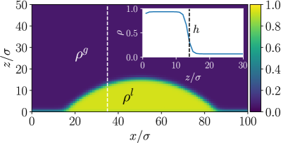
Figure 1: A droplet density profile obtained from lattice DFT in a domain of size $L_{x}\times L_{z}=100\sigma\times 50\sigma$ with lattice spacing $\sigma$ and a wall for $z\leq 0$. The colour-coding for the density scale is given on the right. The inset shows a density profile of a cut through the droplet at the position indicated by the white dashed line. The height $h$ is marked with a black dashed line at the interface between the liquid ($\rho^{l}$) and gas ($\rho^{g}$) phase.

As a result, the minimization of the grand potential $\Omega[\rho(\mathbf{x})]$ with respect to $\rho(\mathbf{x})$ is reduced to a minimization of an effective interface Hamiltonian $F[h(x)]$ with respect to a function $h(x)$ with $x\in[0,L_{x}]$ that describes the position of the liquid-gas interface (cf. Fig. 1). Of course, neither functional is known exactly, but a good approximation for the latter is

$$F\left[h\right]=\int\limits_{0}^{L_{x}}\left[g\big{(}h(x)\big{)}+\gamma_{\mathrm{lg}}\xi+\gamma_{\mathrm{sl}}\right]\mathrm{d}x.$$ (1)

This excess free energy contains contributions from the liquid-gas and solid-liquid interfaces, i.e., the surface tensions $\gamma_{\mathrm{lg}}$ and $\gamma_{\mathrm{sl}}$, and the interaction energy of the two interfaces, i.e., the binding potential $g(h)$. Here $\mathrm{d}s=\xi\mathrm{d}x$ is the local interface element, i.e., $\xi=\sqrt{1+(\partial_{x}h)^{2}}$ represents the interface metric. For small interface slopes one can make the small-gradient or long-wave approximation $\xi\approx 1+(\partial_{x}h)^{2}/2$ often used in gradient dynamics models on the interface Hamiltonian (aka thin film or lubrication models). Oron, Davis, and Bankoff (1997); Thiele (2010); Yin et al. (2017)

The crucial step in the coarse-graining procedure is to determine the binding potential from a set of one-dimensional density profiles $\rho(z)$, where $z$ is the perpendicular distance from the wall, obtained by minimizing $\Omega[\rho(z)]$ under the constraint of fixed adsorptions $\Gamma$ and under the condition that $\mu=\mu_{\mathrm{coex}}$, i.e. that $\rho(z)\to\rho^{g}$ for $z\to\infty$, far from the wall. Since one can define $h=\Gamma/(\rho^{l}-\rho^{g})$, this is equivalent to imposing the film height $h$. As discussed in Ref. Archer and Evans, 2011 for the somewhat related case of droplet nucleation, the adsorption constraint condition can not be implemented through a Lagrange multiplier, since this would shift the chemical potential away from the coexistence value. In Refs. Hughes, Thiele, and Archer, 2015, 2017 the authors employ an iterative Picard algorithm for the minimization of the grand potential, where the adsorption is imposed through a self-consistent calculation of an additional fictitious potential $V_{\mathrm{eff}}(z)$. The a priori unknown $V_{\mathrm{eff}}(z)$ has to be calculated separately for each adsorption and can be interpreted as an additional space-dependent external potential that acts mainly within the liquid, i.e., $V_{\mathrm{eff}}\rightarrow 0$ for $z\rightarrow\infty$. A detailed discussion of the fictitious potential method can be found in Archer and Evans, 2011; Hughes, Thiele, and Archer, 2015.

Here, we present an alternative approach based on the Nudged Elastic Band method Henkelman and Jónsson (2000); Henkelman, Jóhannesson, and Jónsson (2002); Sheppard, Terrell, and Henkelman (2008), also well known as a geometry optimization algorithm used to determine chemical reaction paths. It was successfully employed for a problem similar to that discussed above, namely to determine the free energy barrier for the nucleation of a liquid drop in a gas phase. Lutsko (2008) Originally, the NEB method was introduced to determine saddle points on a potential energy landscape as well as corresponding steepest descent paths (SDP) connecting saddle points and minima.Schlegel (2011) As mentioned above, our aim here is to obtain from DFT the minimum of the grand potential for a specified adsorption and bulk density. The SDP on the free energy landscape (with respect to the Euclidean metric) obtained by the NEB method can be parametrized by the adsorption. The free energy values along the path are interpreted as an approximation for the required constrained free energy minima. We compare our results obtained from the NEB method to the corresponding results obtained via the fictitious potential approach and show that they are in excellent agreement. Furthermore, we verify that the NEB method does in fact give the SDP by additionally comparing to results obtained from a pseudo dynamics (i.e. the trajectory given by a non-conserved dynamical equation based on the DFT). However, we first introduce the DFT.

II Model system

As a simple model system we consider the following discrete lattice DFT grand potential in a reduced one-dimensional (1D) description of a 2D or 3D system (i.e. assuming translation invariance along the wall)

$$\Omega(\{\rho_{i}\})= k_{\mathrm{B}}T\sum\limits_{i=1}^{L_{z}}[\rho_{i}\ln(\rho_{i})+(1-\rho_{i})\ln(1-\rho_{i})]$$ (2)

$$-\frac{1}{2}\sum\limits_{i=1}^{L_{z}}\sum\limits_{j=1}^{L_{z}}\epsilon_{ij}\rho_{i}\rho_{j}+\sum\limits_{i=1}^{L_{z}}\rho_{i}(V_{i}-\mu).$$

Here, $\{\rho_{i}\}$ are the densities in a system of size ${L_{z}}$, $k_{\mathrm{B}}$ is the Boltzmann constant, $T$ is the temperature (in the following $k_{\mathrm{B}}T=\beta^{-1}$), $\mu$ is the chemical potential, $\{V_{i}\}$ is an external potential modeling the wall interaction, whereas the fluid inter-particle interaction is modeled through the interaction matrix $\epsilon_{ij}$. In our case, we consider nearest neighbor (i.e., short-range) interactions as well as particle self-interactions that results from the mapping of the particle pair interactions in the full translation-invariant 2D or 3D system, as described in Ref. Hughes, Thiele, and Archer, 2014. In contrast, the wall potential is long-ranged and acts across the entire system, algebraically decaying as

$$V_{i}=-\epsilon_{\omega}i^{-3}~{}~{}\mathrm{for}~{}i\geq 1,$$ (3)

i.e., implicitly $V_{i}=\infty$ for $i<1$. As a measure of the thickness of the wetting film we define the adsorption on a domain of length ${L_{z}}$ according to:

$$\Gamma=\sum_{i=1}^{L_{z}}\left(\rho_{i}-\rho^{g}\right)$$ (4)

with the resulting effective film height $h=\Gamma/(\rho^{l}-\rho^{g})$.

III Nudged Elastic Band approach

The NEB method belongs to the class of Double-Ended Chain-of-States methods for geometric optimization problems Henkelman and Jónsson (2000); Henkelman, Jóhannesson, and Jónsson (2002); Sheppard, Terrell, and Henkelman (2008); Schlegel (2011), i.e., on a free energy landscape a set of $P$ points is distributed between two fixed end points in such a way that a pre-defined criterion is optimized. Here, these points are represented by a sequence of density profiles $\bm{\rho}^{I}=\{\rho^{I}_{i}\},~{}I=1\dots P$, with corresponding values of the grand potential $\Omega[\bm{\rho}^{I}]$ and adsorption $\Gamma^{I}$. As end points ($\bm{\rho}^{0}$, $\bm{\rho}^{P+1}$) of the chain, we use the density profiles of a homogeneous bulk gas ($\bm{\rho}^{0}=\bm{\rho}^{g}$) at zero adsorption $\Gamma^{0}=0$ and a bulk liquid phase in contact with the wall ($\bm{\rho}^{P+1}=\bm{\rho}^{wl}$) with a corresponding $\Gamma^{P+1}=\Gamma^{wl}$, that minimizes the unconstrained $\Omega[\bm{\rho}]$. As initial guesses for all intermediate profiles we use hyperbolic tangent functions

$$\rho^{I}_{i}=\frac{1}{2}(\rho^{g}-\rho^{l})\mathrm{tanh}\left(i\sigma-a_{I}{L_{z}}\right)+\frac{1}{2},$$ (5)

placing the liquid-gas interface at the desired positions via the parameter $a_{I}$.

An individual optimization process for each single $\Omega[\bm{\rho}^{I}]$ point on the free energy landscape will always reach a minimum of the functional. To prevent this and to well distribute the intermediate profiles $\bm{\rho}^{I}$ between the two end points, an artificial elastic force $\bm{F}^{I}_{\text{elastic}}$ is introduced between profiles. Then the entire chain of elastically joined profiles is optimized in nparallel. The elastic energy is proportional to the squared distance between two neighboring density profiles (based on the $L_{2}$ norm)

$$|\bm{\rho}^{I+1}-\bm{\rho}^{I}|^{2}=\sum_{i=1}^{L_{z}}\left(\rho^{I+1}_{i}-\rho^{I}_{i}\right)^{2}.$$ (6)

Note that if we replace the distance measure between profiles in Eq. (6) by $\sum_{i=1}^{L_{z}}\left|\rho^{I+1}_{i}-\rho^{I}_{i}\right|$ or even the difference between adsorptions $|\Gamma^{I+1}-\Gamma^{I}|$, then the results discussed below do not change. The elastic force only acts along the chain, i.e., it is a parallel force component, whereas the component perpendicular to the chain, results from the energy functional $\bm{F}_{\text{FE}}^{I}=-\partial\Omega(\bm{\rho})/\partial\bm{\rho}|_{\bm{\rho}=\bm{\rho}^{I}}$. Thus, on the discretized space of density profiles, we employ the Euclidean metric in order to approximate the constrained minimum free energies by points on a SDP. The overall force vector $\bm{F}_{\text{NEB}}=\{\bm{F}_{\text{NEB}}^{1},\dots,\bm{F}_{\text{NEB}}^{P}\}$ to be minimized is composed of the forces acting at all intermediate points $I=1\dots P$ (i.e. excluding the end points), where

$$\bm{F}_{\text{NEB}}^{I}=\underline{\bm{P}}^{\parallel}\bm{F}_{\text{elastic}}^{I}+\underline{\bm{P}}{{}^{\perp}}\bm{F}_{\text{FE}}^{I},$$ (7)

with $\underline{\bm{P}}^{\parallel}$ and $\underline{\bm{P}}{{}^{\perp}}$ as projection operators onto the direction parallel and perpendicular to the chain, respectively. The projection operators are obtained via a tangent formalism and the detailed form of $\bm{F}^{I}_{\text{elastic}}$ can be found in Ref. Henkelman and Jónsson, 2000. For the minimization of $|\bm{F}_{\text{NEB}}|$ we employ geometric optimization using direct inversion in the interactive subspace (GDIIS), see Refs. Császár and Pulay, 1984; Farkas and Schlegel, 2002. Ideally, this yields a set of profiles $\bm{\rho}^{I}$ that are homogeneously distributed along the SDP between $\bm{\rho}^{g}$, $\bm{\rho}^{wl}$ and the extrema in between. Since the force vector results from an artificial projection procedure, it is not obvious that this method is guaranteed to give the exact SDP. However, in practice it seems to do very well, as is illustrated next.

IV Comparison of fictitious potential and NEB methods

We use the lattice DFT (2) with the interaction parameters $\beta\epsilon_{ij}=\beta\epsilon=0.95$, the chemical potential fixed at coexistence $\mu=\mu_{\mathrm{coex}}=-5\epsilon/2$ (cf. Ref. Hughes, Thiele, and Archer, 2014) and calculate the binding potentials for two different values of the wall attraction strength parameter $\beta\epsilon_{\omega}$, employing both the fictitious potential method Hughes, Thiele, and Archer (2015) and the NEB method described in the previous section. Fig. 2 (left) shows that the resulting binding potentials agree very well, while Fig. 2 (right) illustrates the agreement of the obtained density profiles.

Figure 2: Left: Comparison of the binding potentials obtained as a function of the adsorption $\Gamma$, as determined by three different methods: fictitious potential method (FP), Nudged Elastic Band method (NEB) and via a pseudo dynamics that follows the steepest descent (SDP) in the energy landscape initiated at $\bm{\rho}^{g}$ and the local maximum (for $\beta\epsilon_{\omega}=0.6$). Two different wall attraction strengths are considered, representing the cases of wetting ($\beta\epsilon_{\omega}=1.2$) and partial wetting ($\beta\epsilon_{\omega}=0.6$). The inset displays the data in a double logarithmic plot to highlight the power law behavior at large film height (the black dashed line shows $0.1\Gamma^{-2}$ for comparison). Right: The corresponding density profiles are shown for adsorptions $\sigma^{2}\Gamma\approx 0.4,2.4$, and $7.8$, which are marked in the left panel by vertical dashed lines and the letters A, B, and C, respectively.

Varying the wall attraction strength parameter $\epsilon_{\omega}$, we see agreement for two different wetting regimes, namely, partial wetting at $\beta\epsilon_{\omega}=0.6$ and complete wetting at $\beta\epsilon_{\omega}=1.2$ – see Ref. Hughes, Thiele, and Archer, 2015 for more on the behavior at the wetting transition. We emphasize that at large adsorption values, both methods yield the power law decay $g(\Gamma)\sim\Gamma^{-2}$ expected in a system with long-range interactions Hughes, Thiele, and Archer (2015, 2017); Dietrich (1988); Dietrich and Napiórkowski (1991); Schick (1990) (here the interaction with the wall), cf. the inset of Fig. 2. Note that in the NEB approach the chain of states is non-equidistant in $\sigma^{2}\Gamma$: the point density is increased in the small adsorption value regime, to obtain a finer resolution where $g(\Gamma)$ is more strongly varying.

In addition to the two methods introduced above, we calculate a SDP employing a pseudo-dynamics that starts at $\Omega\left[\bm{\rho}^{g}\right]$ and at both sides of the local maximum for the partial wetting case (the starting points are obtained by the NEB or the fictitious potential method) and follows the steepest gradient in small steps to $\Gamma\rightarrow\infty$ or to the minimum corresponding to a small finite value of the adsorption at the wall. The resulting path also agrees perfectly with the NEB approach, which is what should be expected if both methods approximate the SDP.

V Conclusion

We have presented a Nudged Elastic Band method for calculating the coarse-grained mesoscopic binding potential $g(h)$ for a liquid film on a solid substrate based on microscopic DFT. The examples we have considered indicate that the method yields results that are indistinguishable from those using the fictitious potential method of Refs. Hughes, Thiele, and Archer, 2017, 2015, which is an approach based on a self-consistent calculation of the fluid density profiles for specified values of the adsorption. Binding potentials obtained with the fictitious potential method were used in Ref. Hughes, Thiele, and Archer, 2017 to calculate drop profiles that agree remarkably well with drop profiles calculated directly using DFT. The agreement of fictitious potential and NEB approach represents an important independent validation of the previous results obtained via the fictitious potential approach which have already recently been employed in mesoscopic gradient dynamics models to compute the spreading dynamics of droplets and the advance of adsorption layers by combining advective and diffusive dynamics.Yin et al. (2017)

Since determining the binding potential involves calculating non-equilibrium states at $\mu=\mu_{\mathrm{coex}}$ through a constrained minimization which cannot be formulated in terms of Lagrange multipliers, it is not a priori obvious that the different approaches should give identical results. The fact that the different approaches are in excellent agreement validates both methods, though we have not rigorously proved that our NEB approach gives the desired constrained minimum free energies.

Besides validating the approach of Refs. Hughes, Thiele, and Archer, 2017, 2015, our present NEB method represents, from a technical point of view, a very efficient way to calculate binding potentials that additionally allows for an intuitive geometric interpretation of the binding potential as ‘tracking’ the Euclidian steepest descent of the grand potential.

The approach can be readily used for calculations based on other microscopic models, e.g., continuum DFT models, to derive coarse-grained mesoscopic binding potentials. Using these in interface Hamiltonians allows for studies of wetting transitions, mesoscopic static droplet shapes and even mesoscopic droplet dynamics. It is a very efficient tool for parameter studies because the entire binding potential is calculated in one single optimization procedure and the point chains (chains of density profiles) obtained for one parameter set can be directly employed as initial guesses for the calculation at neighboring parameter sets. A future challenge consists in extending the presented method to determine binding potentials for complex fluids where it depends not only on film height but also on other, internal, degrees of freedom. This would allow one to provide mesoscopic gradient dynamics models for such fluids Thiele, Todorova, and Lopez (2013); Thiele, Archer, and Pismen (2016) with correct coarse-grained wetting energies.