Selection of the Regularization Parameter in the Ambrosio-Tortorelli Approximation of the Mumford-Shah Functional for Image Segmentation

Abstract

The Ambrosio-Tortorelli functional is a phase-field approximation of the Mumford-Shah functional that has been widely used for image segmentation. The approximation has the advantages of being easy to implement, maintaining the segmentation ability, and $\Gamma$-converging to the Mumford-Shah functional. However, it has been observed in actual computation that the segmentation ability of the Ambrosio-Tortorelli functional varies significantly with different values of the parameter and it even fails to $\Gamma$-converge to the original functional for some cases. In this paper we present an asymptotic analysis on the gradient flow equation of the Ambrosio-Tortorelli functional and show that the functional can have different segmentation behavior for small but finite values of the regularization parameter and eventually loses its segmentation ability as the parameter goes to zero when the input image is treated as a continuous function. This is consistent with the existing observation as well as the numerical examples presented in this work. A selection strategy for the regularization parameter and a scaling procedure for the solution are devised based on the analysis. Numerical results show that they lead to good segmentation of the Ambrosio-Tortorelli functional for real images.

AMS 2010 Mathematics Subject Classification: 65M50, 65M60, 94A08, 35K55

Key words: regularization, image segmentation, phase-field model, moving mesh, mesh adaptation, finite element method

Abbreviated title: Selection of regularization parameter in Ambrosio-Tortorelli functional

1 Introduction

Segmentation for a given image is a process to find the edges of objects and partition the image into separate parts that are relatively smooth. This can be achieved by minimizing some objective functionals and multiple theories have been developed. One of the most commonly used functionals, proposed by Mumford and Shah [27], takes the form

$$E[u,\Gamma]=\frac{\alpha}{2}\int_{\Omega\setminus\Gamma}|\nabla u|^{2}dx+\beta H^{1}(\Gamma)+\frac{\gamma}{2}\int_{\Omega}(u-g)^{2}dx,$$ (1)

where $\Omega$ is a rectangular domain, $\alpha$, $\beta$, and $\gamma$ are positive parameters, $g$ is the grey level of the input image, $u$ is the target image, $\Gamma$ denotes the edges of the objects in the image, and $H^{1}(\Gamma)$ is the one-dimensional Hausdorff measure. Upon minimization, $u$ is close to $g$, $\nabla u$ is small on $\Omega\setminus\Gamma$, and $\Gamma$ is as short as possible. An optimal image is thus close to the original one and almost piecewise constant. Moreover, the terms in (1) represent different and often conflicting objectives, making its minimization and thus image segmentation an interesting but challenging topic to study.

To avoid mathematical difficulties caused by the $H^{1}(\Gamma)$ term, De Giorgi et al. [7] propose an alternative functional as

$$F[u]=\frac{\alpha}{2}\int_{\Omega}|\nabla u|^{2}dx+\beta H^{1}(S_{u})+\frac{\gamma}{2}\int_{\Omega}|u-g|^{2}dx,$$ (2)

where $S_{u}$ is the jump set of $u$. They show that (2) has minimizers in $SBV(\Omega)$ (the space of special functions of bounded variation) and is equivalent to (1) in the sense that if $u\in{\Omega}$ is a minimizer of (2), then $(u,S_{u})$ is a minimizer of (1).

Although it is a perfectly fine functional to study in mathematics, (2) is not easy to implement in actual computation due to the fact that the jump set of the unknown function and its Hausdorff measure are extremely difficult, if not impossible, to compute. To avoid this difficulty, Ambrosio and Tortorelli [1] propose a regularized version as

$$AT_{\epsilon}[u,\phi]=\frac{\alpha}{2}\int_{\Omega}(\phi^{2}+k_{\epsilon})|\nabla u|^{2}dx+\beta\int_{\Omega}\left(\epsilon|\nabla\phi|^{2}+\frac{1}{4\epsilon}(1-\phi)^{2}\right)dx+\frac{\gamma}{2}\int_{\Omega}|u-g|^{2}dx,$$ (3)

where $\epsilon>0$ is the regularization parameter, $k_{\epsilon}=o(\epsilon)$ is a parameter used to prevent the functional from becoming degenerate, and $\phi$ is a new unknown variable which ideally is an approximation of the characteristic function for the jump set of $u$, i.e.,

$$\phi(x)\approx\chi_{u}(x)\equiv\begin{cases}0,\quad&\text{ if }x\in S_{u}\\ 1,\quad&\text{ if }x\notin S_{u}.\end{cases}$$ (4)

They show that $AT_{\epsilon}$ has minimizers $u\in SBV(\Omega)$ and $\phi\in L^{2}(\Omega)$ and $\Gamma$-converges to $F(u)$. $\Gamma$-convergence, first introduced by de Giorgi and Franzoni [8], is a concept that guarantees the minimizer of $AT_{\epsilon}$ converges to that of $F$ as $\epsilon\to 0$.

The first finite element approximation for the functional $AT_{\epsilon}$ is given by Bellettini and Coscia [4]. They seek linear finite element approximations $u_{h}$ and $\phi_{h}$ to minimize

$$AT_{\epsilon,h}[u_{h},\phi_{h}] =\frac{\alpha}{2}\int_{\Omega}(\phi_{h}^{2}+k_{\epsilon})|\nabla u_{h}|^{2}dx+\beta\int_{\Omega}\left(\epsilon|\nabla\phi_{h}|^{2}+\frac{1}{4\epsilon}\pi_{h}((1-\phi_{h})^{2})\right)dx$$

$$+\frac{\gamma}{2}\int_{\Omega}\pi_{h}((u_{h}-g_{\epsilon})^{2})dx,$$ (5)

where $\pi_{h}$ is the linear Lagrange interpolation operator and $g_{\epsilon}$ is a smooth function which converges to $g$ in the $L^{2}$ norm as $\epsilon\to 0$. They show that $AT_{\epsilon,h}$ $\Gamma$-converges to $F(u)$ when the maximum element diameter is chosen as $h=o(\epsilon)$. It should be pointed out that Feng and Prohl [12] have established the existence and uniqueness of the solution to an initial-boundary value problem (IBVP) of the gradient flow equation of (3) and proven that a finite element approximation of the IBVP converges to the continuous solution as the mesh is refined.

It is noted that the Ambrosio-Tortorelli functional (3) is actually a phase-field approximation of the Mumford-Shah functional (1). Phase-field modeling has been used widely in science and engineering to handle sharp interfaces, boundaries, and cracks in numerical simulation of problems such as dendritic crystal growth [22, 35], multiple-fluid hydrodynamics [23, 30, 31, 36], and brittle fracture [5, 13, 26]. It employs a phase-field variable $\phi$, which depends on a regularization parameter $\epsilon$ describing the actual width of the smeared interfaces, to indicate the location of the interfaces. Phase-field modeling has the advantage of being able to handle complex interfaces without relying on their explicit description. Mathematically, phase-field models such as (3) have been studied extensively (e.g., see [1]) for $\Gamma$-convergence. However, few studies have been published for the role of the regularization parameter in actual simulation. It is a common practice that a specific value of $\epsilon$ is used without discussion or explanation in phase-field modeling. Even worse, it has been observed [25, 28, 33] that a phase-field model for brittle fracture simulation does not $\Gamma$-converge as $\epsilon\to 0$ and $\epsilon$ can be interpreted as a material parameter since its choice influences the critical stress. More recently, the choice of $\epsilon$ has been studied in [10] based on physical arguments and with experimental validation.

The objective of this paper is to study the effects and selection of the regularization parameter in the Ambrosio-Tortorelli functional (3) which is a special example of phase-field modeling in image segmentation. We consider the gradient flow equation of $AT_{\epsilon}$ subject to a homogeneous Neumann boundary condition and carry out an asymptotic analysis for the solution of the corresponding IBVP as $\epsilon\to 0$. We show that, when $g$ is continuous, the functional can have different segmentation behavior for small but finite $\epsilon$ and eventually loses its segmentation ability for infinitesimal $\epsilon$. This is consistent with the existing observation in phase-field modeling and with the numerical examples to be presented. The analysis is also used to devise a selection strategy for $\epsilon$ and a scaling for $u$ and $g$. Numerical results with real images confirm that the strategies can lead to good segmentation of $AT_{\epsilon}$ in the sense that $\phi$ is close to the characteristic function of $g$ (cf. (4)).

An outline of the paper is as follows. The asymptotic analysis is given in Section 2, followed by the description of a moving mesh finite element method in Section 3. Illustrative numerical examples are given in Section 4. A selection strategy for $\epsilon$ and a scaling procedure for $u$ and $g$ as well as examples with several real input images are presented in Section 5. Finally, Section 6 contains conclusions.

2 Behavior of the minimizer of $AT_{\epsilon}$ as $\epsilon\to 0$ for continuous $g$

We first explain why we consider $g$ as a continuous function. In image segmentation, the function $g$ represents an image and is given the grey-level values at the pixels. Generally speaking, the values of $g$ at points other than the pixels are needed in finite element computation. These values are computed commonly through (linear) interpolation of the values at the pixels. This means that $g$ is treated as a continuous function in finite element computation and such a treatment is independent of the regularization parameter in the phase-field modeling. Thus we consider $g$ as a continuous function and study the behavior of the minimizer of $AT_{\epsilon}$ as $\epsilon\to 0$ in this section.

To this end, we consider the gradient flow equation of functional (3),

$$\begin{cases}u_{t}=\alpha\nabla\cdot((k_{\epsilon}+\phi^{2})\nabla u)-\gamma(u-g),\\ \phi_{t}=2\beta\epsilon\Delta\phi-\alpha|\nabla u|^{2}\phi+\frac{\beta}{2\epsilon}(1-\phi),\end{cases}\quad x\in\Omega,\;t>0$$ (6)

subject to the homogeneous Neumann boundary condition

$$\frac{\partial u}{\partial n}=\frac{\partial\phi}{\partial n}=0\quad\text{for}\quad x\in\partial\Omega$$ (7)

and the initial condition

$$u(x,0)=u^{0}(x),\quad\phi(x,0)=\phi^{0}(x),\quad x\in\Omega.$$ (8)

This IBVP has been studied and used to find the minimizer of (3) (as a steady-state solution) by a number of researchers. Noticeably, Feng and Prohl [12] have established the existence and uniqueness of the solution of the IBVP and proven that a finite element approximation converges to the continuous solution as the mesh is refined.

By assumption, $g\in C^{0}(\Omega)$. Then we can expect that the solution $u$ and $\phi$ of the IBVP is smooth. To see the behavior of the solution as $\epsilon\to 0$, we consider the asymptotic expansion of $u$ and $\phi$ as

$$u=u^{(0)}+\epsilon u^{(1)}+\epsilon^{2}u^{(2)}+\cdot\cdot\cdot,$$ (9)

$$\phi=\phi^{(0)}+\epsilon\phi^{(1)}+\epsilon^{2}\phi^{(2)}+\cdot\cdot\cdot,$$ (10)

where $u^{(0)},\;u^{(1)},\;...$ and $\phi^{(0)},\;\phi^{(1)},\;...$ are functions independent of $\epsilon$. Inserting these into (6), we get

$$u^{(0)}_{t}+\epsilon u^{(1)}_{t}+O(\epsilon^{2})= \;\alpha\nabla\cdot\left[\left(o(\epsilon)+(\phi^{(0)}+\epsilon\phi^{(1)}+o(\epsilon))^{2}\right)\nabla(u^{(0)}+\epsilon u^{(1)}+O(\epsilon^{2}))\right]$$

$$\qquad-\gamma(u^{(0)}+\epsilon u^{(1)}+O(\epsilon^{2})-g),$$ (11)

$$\phi^{(0)}_{t}+\epsilon\phi^{(1)}_{t}+O(\epsilon^{2})= \;2\beta\epsilon(\Delta\phi^{(0)}+\epsilon\Delta\phi^{(1)}+O(\epsilon^{2}))$$

$$-\alpha\left|\nabla u^{(0)}+\epsilon\nabla u^{(1)}+O(\epsilon^{2})\right|^{2}(\phi^{(0)}+\epsilon\phi^{(1)}+O(\epsilon^{2}))$$

$$+\frac{\beta}{2\epsilon}(1-\phi^{(0)}-\epsilon\phi^{(1)}-O(\epsilon^{2})),$$ (12)

where we have used $k_{\epsilon}=o(\epsilon)$. Collecting the $O(1)$ terms in (11), we have

$$u_{t}^{(0)}=\alpha\Delta u^{(0)}-\gamma(u^{(0)}-g),\quad\text{ in }\Omega.$$ (13)

Similarly, collecting the $O(1/\epsilon)$ terms and $O(1)$ terms in (12) we get

$$\frac{\beta}{2}(1-\phi^{(0)})=0,\qquad\phi^{(0)}_{t}=-\alpha|\nabla u^{(0)}|^{2}\phi^{(0)}-\frac{\beta}{2}\phi^{(1)}.$$

From these we obtain

$$\phi=1-\epsilon\frac{2\alpha}{\beta}|\nabla u^{(0)}|^{2}+O(\epsilon^{2}).$$ (14)

Like $u$, $u^{(0)}$ also satisfies a homogeneous Neumann boundary condition. Since $g\in C^{0}(\Omega)$, it can be shown (e.g., see [11]) that $\nabla u^{(0)}$ is continuous and bounded. Combining this with (14) we conclude that $\phi\to 1$ as $\epsilon\to 0$. Since the boundaries between different objects in $u$ are indicated by $\phi=0$, this implies that $u$ is a single object and there is no segmentation as $\epsilon\to 0$ when $g$ is continuous. Moreover, $u$ and thus $u^{(0)}$ are kept close to $g$ and we can expect $\nabla u^{(0)}$ to be large in the places where $\nabla g$ is large. From (14) we can see that, for small but not infinitesimal $\epsilon$, $\phi$ can become zero at places where $\nabla g$ is large. In this case, the functional will have good segmentation (cf. the numerical examples in Section 4).

The above analysis shows that, when $g$ is continuous, the choice of the regularization parameter in (3) can be crucial for image segmentation: different values of $\epsilon$ can lead to very different segmentation behavior of the functional and its segmentation ability will disappear as $\epsilon\to 0$.

It should be emphasized that the above observation is not in contradiction with the theoretical analysis made in [1] for the $\Gamma$-convergence and segmentation ability of the functional (3). In [1], these properties are analyzed for $u\in SBV(\Omega)$, implicitly implying that $u$ is discontinuous in general. The above analysis has been made under the assumption that $g$ and thus $u$ are continuous although they may have large gradient from place to place.

It is instructive to see some transient behavior of the solution to the gradient flow equation. To simplify, we drop the diffusion term in the second equation in (6) and get

$$\phi_{t}=-\alpha|\nabla u|^{2}\phi+\frac{\beta}{2\epsilon}(1-\phi).$$ (15)

It has been proven in [12] that the solution of (6) satisfies $0\leq\phi\leq 1$. From this we see that the first term on the right-hand side of (15) is nonpositive, which makes $\phi$ decrease, and the second term is nonnegative, making $\phi$ increase. These two terms compete and reach an equilibrium state. Moreover, if $\phi=1$, we have $\phi_{t}=-\alpha|\nabla u|^{2}\leq 0$, meaning that as long as $|\nabla u|\neq 0$, the first term decreases $\phi$ until $\phi_{t}=0$ is reached. Similarly, if $\phi=0$, we have $\phi_{t}=\frac{\beta}{2\epsilon}>0$, which means $\phi$ increases until the system reaches its equilibrium. The equilibrium value of $\phi$ can be obtained by setting the right-hand side of (15) to be zero, i.e.,

$$\phi\approx\frac{\beta}{\beta+2\epsilon\alpha|\nabla u|^{2}}.$$ (16)

Thus, the equilibrium value of $\phi$ is around 1 for smooth regions where $\nabla u$ is small and around 0 on edges where $\nabla u$ is large.

3 The adaptive moving mesh finite element method

In this section we describe an adaptive moving mesh finite element method for solving the gradient flow equation (6). Recall that a crucial requirement for the Ambrosio-Tortorelli approximation (3) of the Mumford-Shah functional is that $\epsilon$ must be small. Since the width of object edges is in the same order of $\epsilon$, the size of the mesh elements around the edges should be in the same order of $\epsilon$ or smaller for any finite element approximation to be meaningful. On the other hand, the mesh elements do not have to be that small within each object where $u$ and $\phi$ are smooth. Thus, mesh adaptation is necessary for the efficiency of the finite element computation. We use here the MMPDE moving mesh method [20, 21] that has been specially designed for time dependent problems.

It should be pointed out that a number of other moving mesh methods have been developed in the past and there is a vast literature in the area. The interested reader is referred to the books or review articles [2, 3, 6, 21, 32] and references therein. Moreover, moving mesh methods have been successfully applied to phase-field models, e.g., see [9, 24, 29, 34, 37, 38, 39].

It is remarked that the spatial domain $\Omega$ is typically a rectangular domain for image segmentation. However, finite element computation is not subject to this restriction. Moreover, we will consider examples in both one and two dimensions for illustrative purpose in the next section. For these reasons, we consider $\Omega$ as a general polygonal domain in $d$-dimensions ($d=1$ and $2$).

3.1 Finite element discretization

We now consider the integration of (6) up to a finite time $t=T$. Denote the time instants by

$$0=t_{0}<t_{1}<...<t_{n_{f}}=T.$$

For the moment, we assume that a simplicial mesh for $\Omega$ is given at these time instants, i.e., $\mathcal{T}_{h}^{n}$, $n=0,...,n_{f}$, which are considered as the deformation from each other and have the same number of the elements ($N$) and the vertices ($N_{v}$) and the same connectivity. Such a mesh is generated using the MMPDE moving mesh strategy to be described in Section 3.2.

For the finite element discretization of (6), the mesh is considered to change linearly between $t_{n}$ and $t_{n+1}$, i.e.,

$$x_{j}(t)=\frac{t-t_{n}}{t_{n+1}-t_{n}}x_{j}^{n+1}+\frac{t_{n+1}-t}{t_{n+1}-t_{n}}x_{j}^{n},\quad j=1,...,N_{v},\quad t\in(t_{n},t_{n+1})$$

where $x_{j}(t)$, $x_{j}^{n}$, and $x_{j}^{n+1}$ ($j=1,...,N_{v}$) denote the coordinates of the vertices of $\mathcal{T}_{h}(t)$, $\mathcal{T}_{h}^{n}$, and $\mathcal{T}_{h}^{n+1}$, respectively. Denote the linear basis function associated with the $j$-th vertex by $\psi_{j}(\cdot,t)$ and let $V_{h}(t)=\text{span}\{\psi_{1},...,\psi_{N_{v}}\}$. Then, the weak formulation for the linear finite element approximation for (6) is to find $u_{h}(\cdot,t)$, $\phi_{h}(\cdot,t)\in V^{h}(t)$, $0<t\leq T$ such that

$$\begin{cases}\int_{\Omega}\frac{\partial u_{h}}{\partial t}vdx=-\alpha\int_{\Omega}(k_{\epsilon}+\phi_{h}^{2})\nabla u_{h}\cdot\nabla vdx-\gamma\int_{\Omega}(u_{h}-g)vdx=0,&\forall v\in V^{h}(t)\\ \int_{\Omega}\frac{\partial\phi_{h}}{\partial t}vdx=-2\beta\epsilon\int_{\Omega}\nabla\phi_{h}\cdot\nabla vdx-\alpha\int_{\Omega}|\nabla u_{h}|^{2}\phi_{h}vdx+\frac{\beta}{2\epsilon}\int_{\Omega}(1-\phi_{h})vdx,&\forall v\in V^{h}(t).\end{cases}$$ (17)

This is almost the same as that for the finite element approximation on a fixed mesh. The main difference lies in time differentiation. To see this, expressing $u_{h}$ into

$$u_{h}(x,t)=\sum_{i=1}^{N_{v}}u_{i}(t)\psi_{i}(x,t)$$ (18)

and differentiating it with respect to time, we get

$$\frac{\partial u_{h}(x,t)}{\partial t}dx=\sum_{i=1}^{Nv}\frac{du_{i}}{dt}\psi_{i}(x,t)+\sum_{i=1}^{Nv}u_{i}(t)\frac{\partial\psi_{i}(x,t)}{\partial t}.$$

It is known (e.g., see [21]) that

$$\frac{\partial\psi_{i}}{\partial t}=-\nabla\psi_{i}\cdot\dot{X},\quad\text{a.e. in }\Omega$$

where

$$\dot{X}=\sum_{i=1}^{N_{v}}\dot{x}_{i}\psi_{i}(x,t)$$

and $\dot{x}_{i}$’s denote the nodal mesh velocities. Combining the above results, we obtain

$$\frac{\partial u_{h}}{\partial t}=\sum_{i=1}^{N_{v}}\frac{du_{i}}{dt}\psi_{i}-\nabla u_{h}\cdot\dot{X}.$$

Similarly,

$$\phi_{h}(x,t)=\sum_{i=1}^{Nv}\phi_{i}(t)\psi_{i}(x,t),\quad\frac{\partial\phi_{h}}{\partial t}=\sum_{i=1}^{N_{v}}\frac{d\phi_{i}}{dt}\psi_{i}-\nabla\phi_{h}\cdot\dot{X}.$$

From these we can see that mesh movement introduces an extra convection term. Inserting these into (17) and taking $v=\psi_{j}$ successively, we can rewrite (17) into an ODE system in the form

$$\begin{cases}M(X)\dot{U}=F(\dot{X},X,\Phi,U,X),\\ M(X)\dot{\Phi}=G(\dot{X},X,\Phi,U,X),\end{cases}$$ (19)

where $M(X)$ is the mass matrix. This system for $U$ and $\Phi$ is integrated from $t_{n}$ to $t_{n+1}$ using the fifth-order Radau IIA method (e.g., see Hairer and Wanner [15]), with a variable time step being selected based on a two-step error estimator [14].

3.2 The MMPDE moving mesh strategy

We now describe the generation of $\mathcal{T}_{h}^{n+1}$ using the MMPDE moving mesh strategy [21]. For this purpose, we denote the physical mesh by $\mathcal{T}_{h}=\{x_{1},...,x_{N_{v}}\}$, the reference computational mesh by $\hat{\mathcal{T}}_{c,h}=\{\hat{\xi}_{1},...,\hat{\xi}_{N_{v}}\}$ (which is chosen as the very initial physical mesh in our computation), and the computational mesh $\mathcal{T}_{c,h}=\{\xi_{1},...,\xi_{N_{v}}\}$. We assume that all of these meshes have the same number of elements and vertices and the same connectivity. Then, for any element $K\in\mathcal{T}_{h}$ there exists a corresponding element $K_{c}\in\mathcal{T}_{c,h}$. We denote the affine mapping between $K_{c}$ and $K$ by $F_{K}$ and its Jacobian matrix by $F_{K}^{\prime}$.

A main idea of the MMPDE moving mesh strategy is to view any adaptive mesh as a uniform one in the metric specified by a certain tensor. A metric tensor (denoted by $\mathbb{M}$) is a symmetric and uniformly positive definite matrix-valued function defined on $\Omega$. In our computation, we choose $\mathbb{M}$ to be a piecewise constant function depending on $u_{h}$ as

$$\mathbb{M}_{K}=\det(|H_{K}|)^{-\frac{1}{d+4}}|H_{K}|,\quad\forall K\in\mathcal{T}_{h}$$ (20)

where $H_{K}$ is a recovered Hessian of $u_{h}$ on element $K$, $|H_{K}|=Q\text{diag}(|\lambda_{1}|,...,|\lambda_{d}|)Q^{T}$, assuming that the eigen-decomposition of $H_{K}$ is $Q\text{diag}(\lambda_{1},...,\lambda_{d})Q^{T}$, and $\det(|H_{K}|)$ is the determinant of $|H_{K}|$. The recovered Hessian in $K$ is obtained by twice differentiating a local quadratic polynomial fitting in the least-squares sense to the nodal values of $u_{h}$ at the neighboring vertices of the element. The form of (20) is known [17] optimal with respect to the $L^{2}$ norm of linear interpolation error. With this choice of $\mathbb{M}$, we hope that the mesh elements are concentrated in the regions of object edges where the curvature of $u$ is large.

The mesh $\mathcal{T}_{h}$ being uniform in metric $\mathbb{M}$ will mean that the volume of $K$ in $\mathbb{M}$ is proportional to the volume of $K_{c}$ with the same proportional constant for all $K\in\mathcal{T}_{h}$ and $K$ measured in $\mathbb{M}$ is similar to $K_{c}$. These requirements can be expressed mathematically as the equidistribution and alignment conditions (e.g., see [21]),

$$|K|\sqrt{\det(\mathbb{M}_{K})}=\frac{\sigma_{h}|K_{c}|}{|\Omega_{c}|},\qquad\forall K\in\mathcal{T}_{h}$$ (21)

$$\frac{1}{d}\text{tr}\left((F_{K}^{\prime})^{-1}\mathbb{M}_{K}^{-1}(F_{K}^{\prime})^{-T}\right)=\det\left((F_{K}^{\prime})^{-1}\mathbb{M}_{K}^{-1}(F_{K}^{\prime})^{-T}\right)^{\frac{1}{d}},\qquad\forall K\in\mathcal{T}_{h}$$ (22)

where $|K|$ and $|K_{c}|$ denote the volume of $K$ and $K_{c}$, respectively, $d$ is the dimension of $\Omega$, $\text{tr}(\cdot)$ denotes the trace of a matrix, and

$$|\Omega_{c}|=\sum_{K_{c}\in\mathcal{T}_{c,h}}|K_{c}|,\qquad\sigma_{h}=\sum\limits_{K\in\mathcal{T}_{h}}|K|\sqrt{\det(\mathbb{M}_{K})}.$$

An energy functional associated with these conditions has been proposed in [16] as

$$I_{h}(\mathcal{T}_{h},\mathcal{T}_{c,h})= \;\theta\sum_{K\in\mathcal{T}_{h}}|K|\sqrt{\det(\mathbb{M}_{K})}\left(\mathbf{\text{tr}}((F_{k}^{\prime})^{-1}\mathbb{M}_{K}^{-1}(F_{K}^{\prime})^{-T})\right)^{\frac{dp}{2}}$$

$$+ \;(1-2\theta)d^{\frac{dp}{2}}\sum_{K\in\mathcal{T}_{h}}|K|\sqrt{\det(\mathbb{M}_{K})}\left(\frac{|K_{c}|}{|K|\sqrt{\det(\mathbb{M}_{K})}}\right)^{p},$$ (23)

where $\theta\in(0,0.5]$ and $p>1$ are two dimensionless parameters. In our computation, we take $\theta=1/3$ and $p=3/2$ which are known experimentally to work well for most problems.

Notice that $I_{h}$ is a function of $\mathcal{T}_{h}$ and $\mathcal{T}_{c,h}$. We can take $\mathcal{T}_{c,h}$ as the reference computational mesh $\hat{\mathcal{T}}_{c,h}$ and minimize $I_{h}$ with respect to $\mathcal{T}_{h}$. With the MMPDE strategy, the minimization is carried out by integrating a modified gradient system of $I_{h}$,

$$\frac{\partial x_{i}}{\partial t}=-\frac{P_{i}}{\tau}\left(\frac{\partial I_{h}}{\partial x_{i}}\right)^{T},\quad i=1,...,N_{v},\quad t\in(t_{n},t_{n+1}]$$ (24)

where $\frac{\partial I_{h}}{\partial x_{i}}$ is a row vector, $P_{i}=\det(\mathbb{M}(x_{i}))^{\frac{p-1}{2}}$ is a positive function chosen to make (24) invariant under the scaling transformation of $\mathbb{M}$, and $\tau>0$ is a positive parameter used to adjust the time scale of mesh movement. Starting from $\mathcal{T}_{h}^{n}$, we can integrate (24) (with proper modifications for the boundary vertices to allow them to slide on the boundary) from $t_{n}$ to $t_{n+1}$ to obtain $\mathcal{T}_{h}^{n+1}$. Special attention may be needed for the computation of the metric tensor that is typically available only at $\mathcal{T}_{h}^{n}$ (the mesh at $t=t_{n}$). During the integration of (24), the location of the physical vertices changes, and the values of $\mathbb{M}$ at these vertices should be updated via interpolation of its values on the vertices of $\mathcal{T}_{h}^{n}$. It is also worth mentioning that the mesh governed by (24) is known [19] to stay nonsingular if it is nonsingular initially.

To avoid the need of constantly updating the metric tensor $\mathbb{M}$ during the integration of the mesh equation, we now consider an indirect approach of minimizing $I_{h}$. In this approach, we choose $\mathcal{T}_{h}=\mathcal{T}_{h}^{n}$ and minimize $I_{h}$ with respect to $\mathcal{T}_{c,h}$. Then the MMPDE for the computational vertices reads as

$$\frac{\partial\xi_{i}}{\partial t}=-\frac{P_{i}}{\tau}\left(\frac{\partial I_{h}}{\partial\xi_{i}}\right)^{T},\quad i=1,...,N_{v},\quad t\in(t_{n},t_{n+1}].$$ (25)

Starting from $\hat{\mathcal{T}}_{c,h}$, this equation can be integrated from $t_{n}$ to $t_{n+1}$ to obtain a new computational mesh $\mathcal{T}_{c,h}^{n+1}$. In our computation, we use Matlab^®  function ode15s, a Numerical Differentiation Formula based integrator, for this purpose. Note that $\mathcal{T}_{h}^{n}$ and $\mathbb{M}=\mathbb{M}^{n}$ are fixed during the integration and $\mathcal{T}_{h}^{n}$ and $\mathcal{T}_{c,h}^{n+1}$ form a correspondence. Denote the correspondence by $\Psi_{h}$, i.e., $\mathcal{T}_{h}^{n}=\Psi_{h}(\mathcal{T}_{c,h}^{n+1})$. Then, the new physical mesh is defined as

$$\mathcal{T}_{h}^{n+1}=\Psi_{h}(\hat{\mathcal{T}}_{c}),$$ (26)

which can be readily computed using linear interpolation.

A benefit of the above $\xi$-formulation is that the derivative $\partial I_{h}/\partial\xi_{i}$ in (25) can be found analytically using the notion of scalar-by-matrix differentiation [18] and has a relatively simple, compact matrix form. Using this, we can rewrite (25) into

$$\frac{\partial\xi_{i}}{\partial t}=\frac{P_{i}}{\tau}\sum_{K\in\omega_{i}}|K|v_{i_{K}}^{K},\quad i=1,...,N_{v}$$ (27)

where $\omega_{i}$ is the patch of the elements containing $x_{i}$ as a vertex, the index $i_{K}$ denotes the local index of $x_{i}$ in $K$, and $v_{i_{K}}^{K}$ is the local velocity contributed by the element $K$ to the partial derivative $\frac{\partial I_{h}}{\partial x_{i}}$. The local velocities on element $K$ are given by

$$\begin{bmatrix}(v_{1}^{K})^{T}\\ \vdots\\ (v_{d}^{K})^{T}\end{bmatrix}=-E_{K}^{-1}\frac{\partial G}{\partial\det(\mathbb{J})}-\frac{\partial G}{\partial\det(\mathbb{J})}\frac{\det(\hat{E}_{K})}{\det(E_{K})}{\hat{E}_{K}}^{-1},\quad v_{0}^{K}=-\sum_{i=1}^{d}v_{d}^{K},$$ (28)

where $E_{K}=[x_{1}^{K}-x_{0}^{K},...,x_{d}^{K}-x_{0}^{K}]$ and $\hat{E}_{K}=[\xi_{1}^{K}-\xi_{0}^{K},...,\xi_{d}^{K}-\xi_{0}^{K}]$ are the edge matrices of $K$ and $K_{c}$, respectively, $\mathbb{J}=(F_{K})^{-1}=\hat{E}_{K}{E_{K}}^{-1}$, $G=G(\mathbb{J},\det(\mathbb{J}),\mathbb{M}_{K})$ is a function associated with the meshing energy functional, and $\partial G/\partial\mathbb{J}$ and $\partial G/\partial\det(\mathbb{J})$ are the partial derivatives of $G$ with respect to the first and second arguments, respectively. For the meshing energy functional (23), we have

$$G=\theta\sqrt{\det(\mathbb{M}_{K})}(\text{tr}(\mathbb{J}\mathbb{M}_{K}^{-1}\mathbb{J}^{T}))^{\frac{dp}{2}}+(1-2\theta)d^{\frac{dp}{2}}\sqrt{\det(\mathbb{M}_{K})}\left(\frac{\det(\mathbb{J})}{\sqrt{\det(\mathbb{M}_{K})}}\right)^{p},$$

$$\frac{\partial G}{\partial\mathbb{J}}=dp\theta\sqrt{\det(\mathbb{M}_{K})}(\text{tr}(\mathbb{J}\mathbb{M}_{K}^{-1}\mathbb{J}^{T}))^{\frac{dp}{2}-1}\mathbb{M}_{K}^{-1}\mathbb{J}^{T},$$

$$\frac{\partial G}{\partial\det(\mathbb{J})}=p(1-2\theta)d^{\frac{dp}{2}}\det(\mathbb{M}_{K})^{\frac{1-p}{2}}\det(\mathbb{J})^{p-1}.$$

4 Numerical results: behavior of $(u,\phi)$ as $\epsilon\to 0$

In this section we present numerical results obtained with the moving mesh finite element method described in the previous section to illustrate the analysis in Section 2. We choose two analytical functions for $g$, with one each in one dimension and two dimensions, to simulate the grey-level values of images. In particular, the sharp jumps in $g$ model the object edges in the image.

 Example 4.1 (1D hyperbolic tangent).

In this example, we take

$$g=0.5(1+\tanh(100(x-0.5))),\quad x\in(0,1)$$ (29)

which has a sharp jump at $x=0.5$. The initial conditions are taken as $u^{0}=g$ and $\phi^{0}=1$. We take $N=200$, $\alpha=0.01$, $\beta=10^{-3}$, $\gamma=10^{-3}$, and $k_{\epsilon}=10^{-9}$. The computed solution at three time instants for $\epsilon=0.1$, $0.01$, and $10^{-5}$ is shown in Fig. 1. It can be seen that the mesh concentrates around and follows the sharp jumps in the solution. This demonstrates the mesh adaptation ability of the MMPDE moving mesh strategy.

Recall that the jump in the solution simulates object edges in a real image and an ideal segmentation should sharpen this jump while smoothing out the regions divided by the jump. The first row of Fig. 1 shows the evolution of $u$ and $\phi$ for $\epsilon=0.1$. One can see that the jump is not sharpened and $u$ is smoothed out on the whole domain as time evolves. This indicates that the Ambrosio-Tortorelli functional with $\epsilon=0.1$ does not provide a good segmentation. The result is shown for a smaller $\epsilon=0.01$ on the second row of the figure. As time evolves, the jump is getting sharper and $u$ becomes piecewise constant essentially, an indication for good image segmentation. However, when $\epsilon$ continues to decrease, as shown on the last row ($\epsilon=10^{-5}$) of Fig. 1, the jump disappears for the time being, $\phi$ approaches to $1$, and $u$ becomes smooth over the whole domain. This implies that the Ambrosio-Tortorelli functional loses its segmentation ability for very small $\epsilon$, consistent with the analysis in Section 2.

It is interesting to see the transient behavior of $\phi$. From the simplified equation (15), we have $\phi_{t}=-\alpha|\nabla u|^{2}\phi$ initially due to the initial condition $\phi=1$. Thus, we expect that $\phi$ decreases initially and this decrease is more significant in the regions where $\nabla u$ is larger. This is confirmed in the numerical results; see Fig. 1(a,d,g). As time evolves, the system reaches an equilibrium state and $\phi$ is approximately given by (16). When $\epsilon$ is not too small and $\nabla u$ is sufficiently large at some places, then $\phi$ can become close to zero at the places and this yields a good segmentation; see the second row of Fig. 1. However, when $\epsilon$ is too small, $\phi$ will essentially become 1 everywhere and the functional loses its segmentation ability (cf. the third row of Fig. 1).

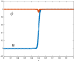
(a) $t=0.005$, $\epsilon=0.1$

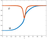
(b) $t=1$, $\epsilon=0.1$

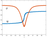
(c) $t=20$, $\epsilon=0.1$

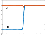
(d) $t=0.005$, $\epsilon=0.01$

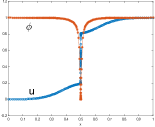
(e) $t=1$, $\epsilon=0.01$

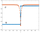
(f) $t=20$, $\epsilon=0.01$

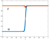
(g) $t=0.005$, $\epsilon=10^{-5}$

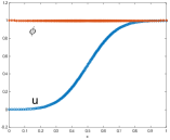
(h) $t=1$, $\epsilon=10^{-5}$

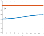
(i) $t=20$, $\epsilon=10^{-5}$

Figure 1: Example 4.1. The computed solution $u_{h}$ and $\phi_{h}$ at three time instants for various values of $\epsilon$. No scaling has been used on $g$ and $u$.

 Example 4.2 (2D hyperbolic tangent).

In this example, we choose

$$g= \,0.49\left[2+\tanh(50(\sqrt{(x-0.5)^{2}+(y-0.5)^{2}}-0.05))\right.$$

$$\qquad\left.-\tanh(50(\sqrt{(x-0.5)^{2}+(y-0.5)^{2}}+0.05))\right],\quad(x,y)\in(0,1)\times(0,1)$$

which models a circle, being close to 0 on the circle and approximately $1$ elsewhere. For the reasons to be explained in Section 5, $u$ and $g$ in the IBVP (6) are scaled in this example according to (31).

We take $u^{0}=g$, $\phi^{0}=1$, $N=2\times 50\times 50$, $\alpha=10^{-3}$, $\gamma=10^{-5}$, $\beta=10^{-2}$, and $k_{\epsilon}=10^{-10}$. The numerical results obtained with $\epsilon=10^{-3}$ and $\epsilon=10^{-7}$ are shown in Figs. 2 and 3, respectively. They show that the mesh concentrates around the jump (the circle) very well, which, once again, demonstrates the mesh adaptation ability of the MMPDE moving mesh method.

Fig. 2 shows that the Ambrosio-Tortorelli functional with $\epsilon=10^{-3}$ makes a good segmentation. The evolution of $\phi$ is given on the first row, and $\phi$ deceases rapidly to $0$ along the circle at $t=7$. The image of the circle is clear as shown on the third row. However, the situation changes when a smaller $\epsilon$ is used. As shown in Fig. 3 with $\epsilon=10^{-7}$, the segmentation ability disappears. As $t$ increases, $\phi$ becomes close to 1 in the whole domain, failing to identify the circle. In the same time, the image of $u$ blurs out. As for Example 4.1, the above observation is consistent with the analysis in Section 2, that is, when $g$ is continuous, the segmentation ability of the Ambrosio-Tortorelli functional varies for small but finite $\epsilon$ and disappears as $\epsilon\to 0$.

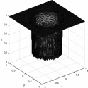
(a) t = 0.00015

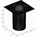
(b) t = 2

(c) t = 7

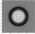
(d) t = 0.00015

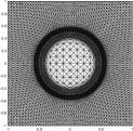
(e) t = 2

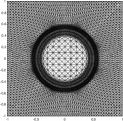
(f) t = 7

(g) t = 0.00015

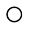
(h) t = 2

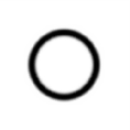
(i) t = 7

Figure 2: Example 4.2. Evolution of the solution for $\epsilon=10^{-3}$. The first, second, and third rows show the evolution of $\phi$, the moving mesh, and the image of $u$, respectively.

(a) t = 0.00015

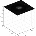
(b) t = 2

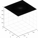
(c) t = 7

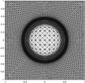
(d) t = 0.00015

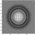
(e) t = 2

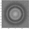
(f) t = 7

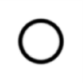
(g) t = 0.00015

(h) t = 2

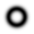
(i) t = 7

Figure 3: Example 4.2. Evolution of the solution for $\epsilon=10^{-7}$. The first, second, and third rows show the evolution of $\phi$, the moving mesh, and the image of $u$, respectively.

5 Selection of the regularization parameter and scaling of $g$ and $u$

5.1 Selection of the regularization parameter

From the analysis in Section 2 and the examples in the previous section, we have seen that it is crucial to choose a proper $\epsilon$ for the Ambrosio-Tortorelli functional to produce a good segmentation when $g$ is continuous. To see how to choose $\epsilon$ properly, we recall that $\phi$ is given in (14) for small $\epsilon$. We want to have $\phi=0$ on object edges. Taking $\phi=0$ in (14) we get

$$\epsilon=\frac{\beta}{2\alpha|\nabla u^{(0)}|^{2}},$$

where $u^{(0)}$ is the solution of (13) subject to a homogeneous Neumann boundary condition. Since $u^{(0)}$ is completely determined by its initial value $g$ and an objective of the Ambrosio-Tortorelli functional is to make $u$ (and thus $u^{(0)}$) close to $g$, it is reasonable to replace $u^{(0)}$ by $g$ in the above formula, i.e.,

$$\epsilon=\frac{\beta}{2\alpha|\nabla g|^{2}}.$$

Since $|\nabla g|$ varies from place to place and $\epsilon$ is a constant, in our computation we replace the former with $(|\nabla g|_{\text{max}}+|\nabla g|_{\text{min}})/2$ and have

$$\epsilon=\frac{\beta}{2\alpha\left((|\nabla g|_{\text{max}}+|\nabla g|_{\text{min}})/2\right)^{2}}.$$ (30)

To demonstrate this choice of $\epsilon$, we apply it to Example 4.1 and obtain $\epsilon=0.008$. The numerical result obtained with the same initial condition and parameters (other than $\epsilon$) is shown in Fig. 4. One can see that this value of $\epsilon$ leads to a good segmentation of the image.

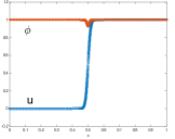
(a) t = 0.005

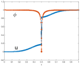
(b) t = 1

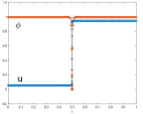
(c) t = 20

Figure 4: Example 4.1. The evolution of $u$ and $\phi$ for $\epsilon=0.008$ (determined by (30)). No scaling has been used on $u$ and $g$.

5.2 Scaling of $g$ and $u$

Our experience shows that (30) works well when the difference in $\nabla g$ between the objects and their edges is sufficiently large. However, when the change of $\nabla g$ is small, the Ambrosio-Tortorelli functional can still fail to produce a segmentation of good quality. To avoid this difficulty, we propose to scale $u$ and $g$ in (6), i.e., $u\to Lu$ and $g\to Lg$ for some parameter $L\geq 1$. This will make the change of $\nabla g$ from place to place more significant. Moreover, the first equation of (6) will stay invariant. The second equation becomes

$$\phi_{t}=2\beta\epsilon\Delta\phi-L^{2}\alpha|\nabla u|^{2}\phi+\frac{\beta}{2\epsilon}(1-\phi),$$

where the second term on the right-hand side is made larger, helping decrease $\phi$. We choose

$$L=\max\left\{1,\frac{|\nabla g|_{\text{cr}}}{|\nabla g|_{\max}}\right\},$$ (31)

where $|\nabla g|_{\text{cr}}$ is a parameter. Generally speaking, the larger $|\nabla g|_{\text{cr}}$ (and $L$) is, the more likely the segmentation works, but this will also make (6) harder to integrate. We take $|\nabla g|_{\text{cr}}=3\times 10^{3}$ (by trial and error) in our computation, unless stated otherwise.

To demonstrate the effects of the scaling, we recompute Example 4.1 with $u^{0}=g=0.5(1+\tanh(20(x-0.5)))$, which has a less steep jump at $x=0.5$ than the function (29). Results with and without scaling are shown in Fig. 5. It can be seen that scaling improves the segmentation ability of the Ambrosio-Tortorelli functional.

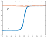
(a) $t=0.005$

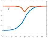
(b) $t=1$

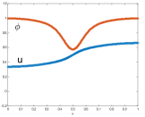
(c) $t=20$

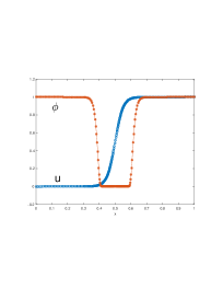
(d) $t=0.005$

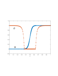
(e) $t=1$

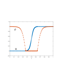
(f) $t=20$

Figure 5: Example 4.1 with $g=0.5(1+\tanh(20(x-0.5)))$ and $u^{0}=g$. $\epsilon$ is chosen as in (30) and other parameters are the same as in Example 4.1. No scaling is used for the top row while the scaling with (31) for $u$ and $g$ is used for the bottom row.

5.3 Segmentation for real images

To further demonstrate the effects of the selection strategy (30) and the scaling (31) we present results obtained for four real images. The results are shown in Figs. 6, 8, 10, and 12 and the corresponding meshes are shown in Figs. 7, 9, 11, and 13, respectively. In these four experiments, $N=2\times 70\times 70$, $\alpha=10^{-3}$, $\gamma=10^{-5}$, $\beta=10^{-2}$, and $k_{\epsilon}=10^{-10}$ are used. A random field in the range $(-0.25,0.25)$ is added to $g$ as well as $u^{0}$. One can observe that the selection strategy (30) for the regularization parameter significantly improves segmentation for all cases.

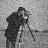
(a) $t=0.005$, $\epsilon=10^{-5}$

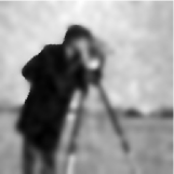
(b) $t=0.16$, $\epsilon=10^{-5}$

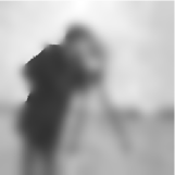
(c) $t=0.6$, $\epsilon=10^{-5}$

(d) $t=0.005$, $\epsilon$ is chosen by (30)

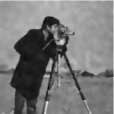
(e) $t=0.16$, $\epsilon$ is chosen by (30)

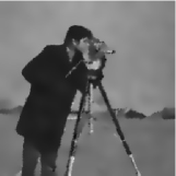
(f) $t=0.6$, $\epsilon$ is chosen by (30)

Figure 6: A comparison of the image segmentation with different $\epsilon$ values.

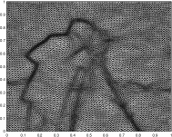
(a) $t=0.005$, $\epsilon=10^{-5}$

(b) $t=0.6$, $\epsilon=10^{-5}$

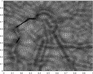
(c) $t=0.6$, $\epsilon=10^{-5}$

(d) $t=0.005$, $\epsilon$ is chosen by (30)

(e) $t=0.16$, $\epsilon$ is chosen by (30)

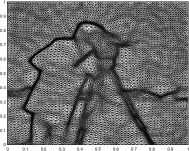
(f) $t=0.6$, $\epsilon$ is chosen by (30)

Figure 7: The meshes corresponding to Fig. 6.

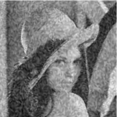
(a) $t=6\times 10^{-6}$, $\epsilon=10^{-6}$

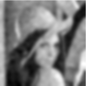
(b) $t=0.15$, $\epsilon=10^{-6}$

(c) $t=0.3$, $\epsilon=10^{-6}$

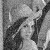
(d) $t=6\times 10^{-6}$, $\epsilon$ is chosen by (30)

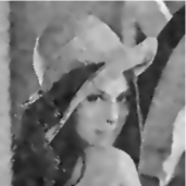
(e) $t=0.15$, $\epsilon$ is chosen by (30)

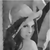
(f) $t=0.3$, $\epsilon$ is chosen by (30)

Figure 8: Evolution of the image.

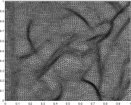
(a) $t=6\times 10^{-6}$, $\epsilon=10^{-6}$

(b) $t=0.15$, $\epsilon=10^{-6}$

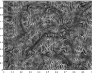
(c) $t=0.3$, $\epsilon=10^{-6}$

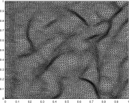
(d) $t=6\times 10^{-6}$, $\epsilon$ is chosen by (30)

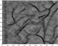
(e) $t=0.15$, $\epsilon$ is chosen by (30)

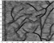
(f) $t=0.3$, $\epsilon$ is chosen by (30)

Figure 9: The meshes corresponding to Fig. 8.

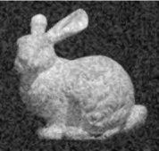
(a) $t=0.002$, $\epsilon=10^{-7}$

(b) $t=0.008$, $\epsilon=10^{-7}$

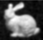
(c) $t=0.2$, $\epsilon=10^{-7}$

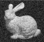
(d) $t=0.002$, $\epsilon$ is chosen by (30)

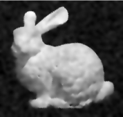
(e) $t=0.008$, $\epsilon$ is chosen by (30)

(f) $t=0.2$, $\epsilon$ is chosen by (30)

Figure 10: Evolution of the image.

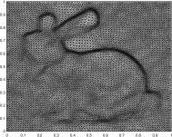
(a) $t=0.002$, $\epsilon=10^{-7}$

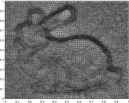
(b) $t=0.008$, $\epsilon=10^{-7}$

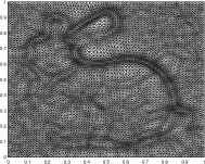
(c) $t=0.2$, $\epsilon=10^{-7}$

(d) $t=0.002$, $\epsilon$ is chosen by (30)

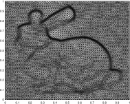
(e) $t=0.008$, $\epsilon$ is chosen by (30)

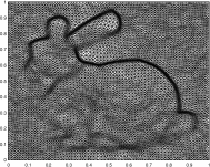
(f) $t=0.2$, $\epsilon$ is chosen by (30)

Figure 11: The meshes corresponding to Fig. 10.

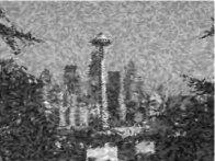
(a) $t=0.00013$, $\epsilon=10^{-7}$

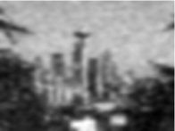
(b) $t=0.08$, $\epsilon=10^{-7}$

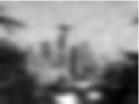
(c) $t=0.3$, $\epsilon=10^{-7}$

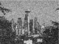
(d) $t=0.00013$, $\epsilon$ is chosen by (30)

(e) $t=0.08$, $\epsilon$ is chosen by (30)

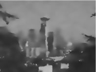
(f) $t=0.3$, $\epsilon$ is chosen by (30)

Figure 12: Evolution of the image.

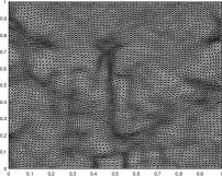
(a) $t=0.00013$, $\epsilon=10^{-7}$

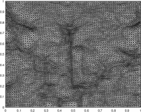
(b) $t=0.08$, $\epsilon=10^{-7}$

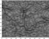
(c) $t=0.3$, $\epsilon=10^{-7}$

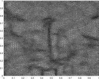
(d) $t=0.00013$, $\epsilon$ is chosen by (30)

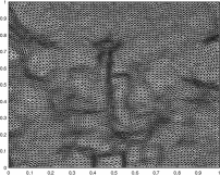
(e) $t=0.08$, $\epsilon$ is chosen by (30)

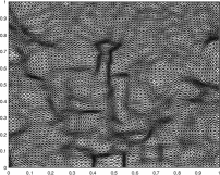
(f) $t=0.3$, $\epsilon$ is chosen by (30)

Figure 13: The meshes corresponding to Fig. 12.

6 Conclusions

The Mumford-Shah functional has been widely used for image segmentation. Its Ambrosio-Tortorelli Approximation has been known for its relative ease in implementation, segmentation ability, and $\Gamma$-convergence to the Mumford-Shah functional as the regularization parameter $\epsilon$ goes to zero. The segmentation ability is based on the assumption that the input image $g$ is discontinuous across the boundaries between different objects, and this discontinuity must be maintained in the limit of $\epsilon\to 0$ during numerical computation to retain the $\Gamma$-convergence and the segmentation ability for infinitesimal $\epsilon$ (e.g., see [4]). However, the maintenance of discontinuity in $g$ is often forgotten and $g$ is treated implicitly as a continuous function in actual computation. As a consequence, it has been observed that the segmentation ability of the Ambrosio-Tortorelli functional varies significantly with different values of $\epsilon$ and the functional can even fail to $\Gamma$-converge to the original functional for some cases. Moreover, there exist very few published numerical studies on the behavior of the functional as $\epsilon\to 0$.

We have presented in Section 2 an asymptotic analysis on the gradient flow equation of the Ambrosio-Tortorelli functional as $\epsilon\to 0$ for continuous $g$. The analysis shows that the functional can have different segmentation behavior for small but finite $\epsilon$ and eventually loses its segmentation ability for infinitesimal $\epsilon$. This is consistent with the existing observations in the literature and the numerical examples in one and two spatial dimensions presented in Section 4. Based on the analysis, we have proposed a selection strategy for $\epsilon$ and a scaling procedure for $u$ and $g$ in Section 5. Numerical results with real images show that they lead to a good segmentation of the Ambrosio-Tortorelli functional.

Finally, we recall that the Ambrosio-Tortorelli functional is a special example of phase-field modeling for image segmentation. We hope that the analysis and the selection strategy for the regularization parameter presented in this work can also apply to other phase-field models. We are specially interested in the phase-field modeling of brittle fracture (e.g., see [5, 13, 26]). Investigations in this direction are currently underway.

References

- [1] L. Ambrosio and V. M. Tortorelli. On the approximation of free discontinuity problems. Boll. Un. Mat. Ital. B, 6:105–123, 1992.
- [2] M. J. Baines. Moving Finite Elements. Oxford University Press, Oxford, 1994.
- [3] M. J. Baines, M. E. Hubbard, and P. K. Jimack. Velocity-based moving mesh methods for nonlinear partial differential equations. Commun. Comput. Phys., 10:509–576, 2011.
- [4] G. Bellettini and A. Coscia. Discrete approximation of a free discontinuity problem. Numer. Funct. Anal. Optim., 15:201–224, 1994.
- [5] B. Bourdin, G. A. Francfort, and J. J. Marigo. Numerical experiments in revisited brittle fracture. J. Mech. Phys. Solids, 48:797–826, 2000.
- [6] C. J. Budd, W. Huang, and R. D. Russell. Adaptivity with moving grids. Acta Numerica, 18:111–241, 2009.
- [7] E. De Giorgi, M. Carriero, and A. Leaci. Existence theorem for a minimum problem with free discontinuity set. Arch. Rational Mech. Anal., 108:195–218, 1989.
- [8] E. De Giorgi and T. Franzoni. Su un tipo di convergenza variazionale. Atti Accad. Naz. Lincei Rend. Cl. Sci. Fis. Mat. Natur., 58:842–850, 1975.
- [9] Q. Du and J. Zhang. Adaptive finite element method for a phase field bending elasticity model of vesicle membrane deformations. SIAM J. Sci. Comput., 30:1634–1657, 2008.
- [10] T. T. Nguyen, J. Yvonnet, M. Bornert, C. Chateau, K. Sab, R. Romani, and R. Le Roy. On the choice of parameters in the phase field method for simulating crack initiation with experimental validation. Int J Fract, 197:213–226, 2016.
- [11] L. C. Evans. Partial Differential Equations. American Mathematical Society, Providence, Rhode Island, 1998. Graduate Studies in Mathematics, Volume 19.
- [12] X. Feng and A. Prohl. Analysis of gradient flow of a regularized Mumford-Shah functional for image segmentation and image inpainting. M2AN Math. Model. Numer. Anal., 38:291–320, 2004.
- [13] G. A. Francfort and J. J. Marigo. Revisiting brittle fracture as an energy minimization problem. J. Mech. Phys. Solids, 46:1319–1342, 1998.
- [14] S. González-Pinto, J. I. Montijano, and S. Pérez-Rodríguez. Two-step error estimators for implicit Runge-Kutta methods applied to stiff systems. ACM Trans. Math. Software, 30:1–18, 2004.
- [15] E. Hairer and G. Wanner. Solving Ordinary Differential Equations. II, volume 14 of Springer Series in Computational Mathematics. Springer-Verlag, Berlin, second edition, 1996. Stiff and differential-algebraic problems.
- [16] W. Huang. Variational mesh adaptation: isotropy and equidistribution. J. Comput. Phys., 174:903–924, 2001.
- [17] W. Huang. Metric tensors for anisotropic mesh generation. J. Comput. Phys., 204:633–665, 2005.
- [18] W. Huang and L. Kamenski. A geometric discretization and a simple implementation for variational mesh generation and adaptation. J. Comput. Phys., 301:322–337, 2015. (arXiv:1410.7872).
- [19] W. Huang and L. Kamenski. On the mesh nonsingularity of the moving mesh PDE method. Math. Comp., to appear. (arXiv:1512.04971).
- [20] W. Huang, Y. Ren, and R. D. Russell. Moving mesh partial differential equations (MMPDEs) based upon the equidistribution principle. SIAM J. Numer. Anal., 31:709–730, 1994.
- [21] W. Huang and R. D. Russell. Adaptive Moving Mesh Methods. Springer, New York, 2011. Applied Mathematical Sciences Series, Vol. 174.
- [22] R. Kobayashi. Modeling and numerical simulations of dendritic crystal growth. Physica D, 63:410–423, 1993.
- [23] C. Liu and J. Shen. A phase field model for the mixture of two incompressible fluids and its approximation by a Fourier-spectral method. Phys. D, 179:211–228, 2003.
- [24] J. A. Mackenzie and M. L. Robertson. A moving mesh method for the solution of the one-dimensional phase-field equations. J. Comput. Phys., 181:526–544, 2002.
- [25] S. May, J. Vigonellet, and R. de Borst. A numerical assessment of phase-field models for brittle and cohesive fracture: -covergence and stress oscillations. European J. Mech. A/Solids., 52:72–84, 2015.
- [26] C. Miehe, F. Welschinger, and M. Hofacker. Thermodynamically consistent phase-field models of fracture: Variational principles and multi-field FE implementations. Int. J. Numer. Meth. Eng., 83:1273–1311, 2010.
- [27] D. Mumford and J. Shah. Optimal approximations by piecewise smooth functions and associated variational problems. Commun. Pure Appl. Math, 42:577–685, 1989.
- [28] K. Pham, H. Amor, J.-J. Marigo, and C. Maurini. Gradient damage models and their use to approximate brittle fracture. Int. J. Damage Mech., 20:618–652, 2011.
- [29] J. Shen and X. Yang. An efficient moving mesh spectral method for the phase-field model of two-phase flows. J. Comput. Phys., 228:2978–2992, 2009.
- [30] J. Shen and X. Yang. Decoupled energy stable schemes for phase-field models of two-phase complex fluids. SIAM J. Sci. Comput., 36:B122–B145, 2014.
- [31] J. Shen, X. Yang, and H. Yu. Efficient energy stable numerical schemes for a phase field moving contact line model. J. Comput. Phys., 284:617–630, 2015.
- [32] T. Tang. Moving mesh methods for computational fluid dynamics flow and transport. In Recent Advances in Adaptive Computation (Hangzhou, 2004), volume 383 of AMS Contemporary Mathematics, pages 141–173. Amer. Math. Soc., Providence, RI, 2005.
- [33] J. Vignollet, S. May, R. de Borst, and C. V. Verhoosel. Phase-field models for brittle and cohesive fracture. Meccanica, 49:2587–2601, 2014.
- [34] H. Wang, R. Li, and T. Tang. Efficient computation of dendritic growth with -adaptive finite element methods. J. Comput. Phys., 227:5984–6000, 2008.
- [35] A. A. Wheeler, B. T. Murray, and R. J. Schaefer. Computation of dendrites using a phase field model. Physica D, 66:243–262, 1993.
- [36] X. Yang, J. J. Feng, C. Liu, and J. Shen. Numerical simulations of jet pinching-off and drop formation using an energetic variational phase-field method. J. Comput. Phys., 218:417–428, 2006.
- [37] X. Yang, J. J. Feng, C. Liu, and J. Shen. Numerical simulations of jet pinching-off and drop formation using an energetic variational phase-field method. J. Comput. Phys., 218:417–428, 2006.
- [38] P. Yu, L. Q. Chen, and Q. Du. Applications of moving mesh methods to the Fourier spectral approximations of phase-field equations. In Recent Advances in Computational Sciences, pages 80–99. World Sci. Publ., Hackensack, NJ, 2008.
- [39] F. Zhang, W. Huang, X. Li, and S. Zhang. Moving mesh finite element simulation for phase-field modeling of brittle fracture and convergence of Newton’s iteration. (submitted, 2017) (arXiv:1706.05449).