Control-Data Separation with Decentralized Edge
Control in Fog-Assisted Uplink Communications

Abstract

Fog-aided network architectures for 5G systems encompass wireless edge nodes, referred to as remote radio systems (RRSs), as well as remote cloud center (RCC) processors, which are connected to the RRSs via a fronthaul access network. RRSs and RCC are operated via Network Functions Virtualization (NFV), enabling a flexible split of network functionalities that adapts to network parameters such as fronthaul latency and capacity. This work focuses on uplink communications and investigates the cloud-edge allocation of two important network functions, namely the control functionality of rate selection and the data-plane function of decoding. Three functional splits are considered: (i) Distributed Radio Access Network (D-RAN), in which both functions are implemented in a decentralized way at the RRSs; (ii) Cloud RAN (C-RAN), in which instead both functions are carried out centrally at the RCC; and (iii) a new functional split, referred to as Fog RAN (F-RAN), with separate decentralized edge control and centralized cloud data processing. The model under study consists of a time-varying uplink channel in which the RCC has global but delayed channel state information (CSI) due to fronthaul latency, while the RRSs have local but more timely CSI. Using the adaptive sum-rate as the performance criterion, it is concluded that the F-RAN architecture can provide significant gains in the presence of user mobility.

I Introduction

The evolution of the wireless network architecture traces a line from the decentralized implementation of control and data functionalities in conventional Distributed Radio Access Network (D-RAN) through the centralization of the protocol stack in Cloud-RAN (C-RAN) [ChinaMobile13, ChinaMobileNFGI] to the more recent fog-aided proposals with flexible functional splits between cloud and edge nodes [5GNORMA]. An important motivation for the latest shift to fog-aided solutions is the realization that a fully centralized C-RAN system entails significant, and possibly prohibitive, requirements on the fronthaul connections between edge nodes and cloud, see, e.g., [Fettweis14SPMAG, Simeone16JCN] and references therein. Furthermore, the development of the Network Functions Virtualization (NFV) technology makes adaptive cloud-edge functional splits realizable via software [Rost17arXiv].

The demarcation line between the functionalities to be implemented at the cloud and at the edge is typically drawn to include a given number of physical-layer functions at the edge nodes, such as synchronization, FFT/IFFT and resource demapping [Fettweis14SPMAG, Chang16ICC]. The body of work concerned with edge-cloud functional splits generally aims at assessing the trade-off between performance and fronthaul capacity overhead of different demarcation lines.

In light of these developments, references [Dotsch13Bell, Rost2014WCL, Khalili16TETT] explore the application of the data-control separation architecture [Tafazolli15CST] as the guiding principle underlying the separation of functionalities between edge and cloud with the aim of addressing fronthaul latency limitations. Specifically, [Dotsch13Bell] puts forth the idea of performing the control decisions of the uplink hybrid automatic repeat request (HARQ) protocol at an edge node, while keeping the computationally expensive operation of data decoding at the cloud processor. As shown in [Rost2014WCL, Khalili16TETT, Gulati16VTC], this approach can yield significant reductions in transmission latency thanks to the capability of the edge nodes to provide quick feedback to the mobile users with limited fronthaul overhead.

An important lesson learned from [Dotsch13Bell, Rost2014WCL, Khalili16TETT, Gulati16VTC] is that the implementation of some control functionalities at the edge can be an enabler for the reduction of transmission latency even in the presence of significant delays on the fronthaul links. A work that provides related insights in the different set-up of a multi-hop network with orthogonal links is [Johnston15ISIT]. Reference [Johnston15ISIT] shows that centralized scheduling based on delayed channel state information (CSI) can be outperformed by local scheduling decisions, as long as each network node has more current CSI of its incoming and outgoing links with respect to the centralized scheduler.

In this work, as illustrated in Fig. 1, we study the optimal functional split of control and data plane functionalities at the edge nodes, referred to as remote radio systems (RRSs) [ChinaMobileNFGI], and at the cloud, referred to as remote cloud center (RCC) [ChinaMobileNFGI], for uplink communication. We specifically focus on the following functionalities: (i) the control plane functionality of the data rate selection, and (ii) the data plane functionality of data decoding. We aim at assessing the impact of fronthaul latency on the relative performance of different splits, whereby rate selection and data decoding may be performed separately at either cloud or edge.

As summarized in Fig. 1, we specifically consider three functional splits: (i) D-RAN, in which both rate selection and data decoding are implemented at each edge; (ii) C-RAN, whereby both rate selection and data decoding are instantiated at cloud; and (iii) Fog-RAN (F-RAN), whereby the control function of rate selection is performed at the edge, while data decoding is implemented at cloud. The latter functional split is studied here for the first time. The approach is motivated by the idea discussed above of leveraging decentralized control to counteract fronthaul delays. We remark that the label “F-RAN” has been used in works such as [Sengupta16arXiv] to indicate systems with decentralized caching at the RRSs and centralized processing at the RCC. Here we suggest to use the term more generally to describe fog-based solutions involving both cloud and edge operations.

As seen in Fig. 2, the model under study consists of a time-varying uplink channel in which the RCC processor has global but delayed CSI due to fronthaul latency, while the RRSs have local CSI with a lower delay. Using the adaptive sum-rate as the performance criterion (see, e.g., [SreekumarTIT15]), the mentioned functional splits based on the control-data separation architecture are compared through analysis and numerical results.

The rest of the paper is organized as follows. We describe the system model and performance metric in Sec. II. We analyze the three radio access network architectures in Fig. 1 for different control-data functional splits between RCC and RRSs: D-RAN in Sec. III, C-RAN in Sec. IV, and F-RAN in Sec. LABEL:Sec:F-RAN. In Sec. LABEL:Sec:Numerical, numerical results are presented. Concluding remarks are summarized in Sec. LABEL:Sec:Conclusion.

         
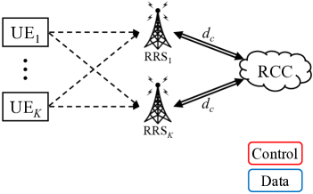
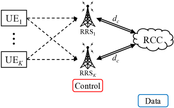
        (a) D-RAN                                               (b) C-RAN                                                             (c) F-RAN                     

Figure 1: Three radio access network architectures for different control-data functional splits between cloud and edge: (a) D-RAN, (b) C-RAN, and (c) F-RAN.

II System Model and Performance Metric

We consider the uplink of a fog-assisted system illustrated in Fig. 2, which consists of $K$ remote radio systems (RRSs), a remote cloud center (RCC), and $K$ active user equipments (UEs). We assume that user-cell association has been carried out, so that each UE $i$ is associated to a given RRS $i$, and we have the same number of active UEs and RRSs. We denote the set of all UEs and RRSs as $\mathcal{K}=\{1,\dots,K\}$. As further detailed below and illustrated in Fig. 1, we consider three different cloud-edge splits, namely: (i) D-RAN: The RCC is not present and both rate selection and data decoding for UE $k$ are carried out at RRS $k$; (ii) C-RAN: The RCC implements both rate selection and data decoding for all UEs; (iii) F-RAN: In this novel functional split, the RRS $k$ performs rate selection for UE $k$ while data decoding for all UEs is performed at the RCC.

An important role in the analysis is played by the timeliness of the CSI available at the RRS and RCC at the time of rate selection. In particular, as illustrated in Fig. 3, for D-RAN and F-RAN, we assume that the latency between uplink training transmission or CSI feedback and the time slot allocated for uplink transmission equals $d_{e}$ time slots of the wireless channel. As an example, the latency contributions for uplink transmission in LTE Release 14 [LTERel14Latency] are Scheduling Request (SR) periodicity, uplink scheduling delay and uplink grant transmission. For a transmission time interval (TTI) of, say, $0.5$$-$$1$ ms, the latency $d_{e}$ can be large as $1$$-$$2$ slots [LTERel14Latency]. For C-RAN, in addition to the delay $d_{e}$, one needs to consider the two-way communication between RRSs and RCC on the fronthaul. This entails a latency equal to $d_{c}$ time slots. The fronthaul transport latency is reported to be around $0.25$ ms in [NGMNOnline] for single-hop fronthaul links and can amount to multiple milliseconds in the presence of multihop fronthauling, while fronthaul-related processing at the RCC can take fractions to a few milliseconds [Nikaein15CONF]. As a result, for TTI of $0.5$$-$$1$ ms, the RCC CSI latency $d_{c}$ can be as large as $3$$-$$5$ slots.

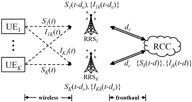
Figure 2: Uplink of the considered fog-assisted system. Communication on the fronthaul links entails a two-way latency of $d_{c}$ time slots (of the wireless interface), while the time elapsed between CSI measurement at the edge and uplink scheduling is $d_{e}$ time slots. The figure indicates the CSI available when selecting the rates for transmitting in slot $t$ at the RRSs for D-RAN and F-RAN and at the RCC for C-RAN. Note that the CSI available for decoding can be assumed to be timely since it can be estimated from pilots included in the data frame, as seen in Fig. 3.

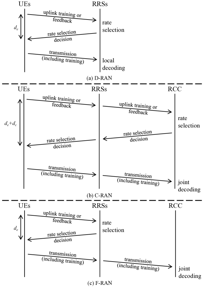
Figure 3: Protocol timeline (time increasing from top to bottom) for: (a) D-RAN; (b) C-RAN; and (c) F-RAN. For D-RAN (a) and F-RAN (c), the latency between uplink training transmission or CSI feedback and the time slot allocated for uplink transmission equals $d_{e}$ time slots of the wireless channel. For C-RAN (b), in addition to the scheduling delay $d_{e}$, one needs to consider the latency associated with two-way fronthaul communication between RRSs and RCC, which equals $d_{c}$ time slots.

II-A Channel Model

At each time slot $t$, the instantaneous power received at RRS $i$ from UE $i$ is denoted as $S_{i}(t)$, while the received power for the cross-channel between an UE $i$ and the RRS $j\neq i$ is denoted as $I_{ji}(t)$. These are assumed to vary across the time index $t=1,2,\dots,T$, which runs over the transmission intervals, according to a Markov model. This model can be obtained, for instance, by approximating the standard Clarke’s model via quantization, see, e.g., [Wang95TVT]. The channel matrix between the UEs and the RRSs at any channel use $k$ of the transmission interval $t=1,2,\dots,T$ can be written as

$${\bf{H}}(t,k)=[{\bf{h}}_{1}^{T}(t,k),\dots,{\bf{h}}_{K}^{T}(t,k)]^{T},$$ (1)

with ${\bf{h}}_{j}(t,k)=[\sqrt{I_{j1}(t)}e^{j\theta_{j1}(t,k)},\dots,\sqrt{S_{j}(t)}e^{j\theta_{jj}(t,k)},\dots,\sqrt{I_{jK}(t)}e^{j\theta_{jK}(t,k)}]$, where the phases $\theta_{ji}(t,k)$ are uniformly distributed in the interval $[0,2\pi)$, mutually independent as per the standard Rayleigh fading model, and vary in an ergodic manner over the channel use index $k$ within each transmission interval $t$.

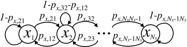
Figure 4: Markov model for the direct channel and cross-channel instantaneous power processes with $N_{x}$ states for $x\in\{S,I\}$ [Wang95TVT].

As illustrated in Fig. 4, the direct instantaneous fading power $S_{i}(t)$ can take $N_{S}$ values, indexed in ascending order as $\{S_{1},\dots,S_{N_{S}}\}$, and is governed by a Markov chain with transition probabilities $p_{S,mn}=\textrm{Pr}[S_{i}(t+1)=S_{m}|S_{i}(t)=S_{n}]$. In a similar manner, the cross-channel power $I_{ji}(t)$ can take $N_{I}$ values, indexed in ascending order as $\{I_{1},\dots,I_{N_{I}}\}$, and varies according to a Markov chain with transition probabilities $p_{I,mn}=\textrm{Pr}[I_{ji}(t+1)=I_{m}|I_{ji}(t)=I_{n}]$. We denote the set of all states for the direct channel as $\mathcal{N}_{S}=\{S_{1},\dots,S_{N_{S}}\}$ and for the cross-channel as $\mathcal{N}_{I}=\{I_{1},\dots,I_{N_{I}}\}$. We recall that Markovian models are widely adopted for the evaluation of the performance of wireless systems (see, e.g., [Wang95TVT, Wei10TVT, Zheng13TWC]). Note that, as in [Wang95TVT], channel variations can only occur between adjacent states, i.e., $p_{x,mn}=0$ if $|m-n|>1$ for $x\in\{S,I\}$. Details on the quantization process from Clarke’s model, which is assumed for the numerical results presented in Sec. LABEL:Sec:Numerical, can be found in Appendix LABEL:Appendix:_Finite_state_Markov_channel.

We conclude this subsection by introducing some useful notation. According to the adopted Markov model, the probability that the direct channel state changes from state $S_{n}$ to the state $S_{m}$, for $S_{m},S_{n}\in\mathcal{N}_{S}$, after $d$ transmission intervals can be written as

$${\textrm{Pr}}\left[S_{i}(t)=S_{m}|S_{i}(t-d)=S_{n}\right]=\beta_{S}^{m|n}(d),$$ (2)

where the probability $\beta_{S}^{m|n}(d)$ is obtained as the $(m,n)$ entry of the matrix ${\bf{T}}_{S}^{d}$, with the transition matrix ${\bf{T}}_{S}$ having $p_{S,mn}$ as the $(m,n)$ entry, i.e., $[{\bf{T}}_{S}]_{m,n}=p_{S,mn}$. Moreover, the stationary probability $\pi_{S,m}$ for the state $S_{m}$ is obtained by solving the linear system as (see, e.g., [MarkovChainBook])

$$\pi_{S,m}=\sum_{S_{n}\in\mathcal{N}_{S}}\pi_{S,n}p_{S,mn},$$ (3)

for $S_{m}\in\mathcal{N}_{S}$. Analogously, we define $\beta_{I}^{m|n}(d)$ as the $d$-step transition probability for the interference process, i.e., ${\textrm{Pr}}\left[I_{ji}(t)=I_{m}|I_{ji}(t-d)=I_{n}\right]=\beta_{I}^{m|n}(d)$ with $m,I_{n}\in\mathcal{N}_{I}$, and $\pi_{I,m}$ as the steady-state probability of the interference process, i.e., $\pi_{I,m}=\sum_{I_{n}\in\mathcal{N}_{I}}\pi_{I,n}p_{I,mn}$ for $I_{m}\in\mathcal{N}_{I}$. We also use the notation $\pi_{\bf{S}}=\prod_{m\in\mathcal{K}}\pi_{S,m}$ for the joint stationary probability of any given direct channel vector ${\bf{S}}\in\mathcal{N}_{S}^{K}$ and we also define $\pi_{\bf{I}}=\prod_{i\in\mathcal{K}}\prod_{j\in\mathcal{K},j\neq i}\pi_{I,I_{ji}}$ for the joint stationary probability of any given cross channel vector ${\bf{I}}\in\mathcal{N}_{S}^{K-1\times K}$.

II-B Cloud-Edge Functional Splits

As discussed, we focus on the control functionality of rate adaptation, or adaptive modulation and coding, that is, the selection of the transmission rates $R_{j}$ (bit/s/Hz) for any UE $j\in\mathcal{K}$, and on the data plane functionality of data decoding. The three control-data functional splits under study (see Fig. 1) are formalized below.
$\bullet$ Distributed Radio Access Network (D-RAN): D-RAN amounts to the most conventional cellular implementation in which control and data plane functionalities are carried out at the RRSs, that is, at the edge. Accordingly, for each time slot $t$, each RRS $j$ selects rate $R_{j}$ for UE $j$ on the basis of local delayed CSI about the direct channel $S_{j}(t-d_{e})$ and about the cross channel ${\bf{I}}_{j}(t-d_{e})$ from all other UEs to the RRS $j$. This information can be obtained, e.g., by means of uplink training in a Time Division Duplex system or via feedback with Frequency Division Duplex (FDD). Moreover, each RRS $j$ individually performs decentralized local data decoding of the signal transmitted by UE $j$ by treating interference as noise. Since data packets are assumed to include training signals, we assume that channel decoding at each RRS can leverage current CSI about the data packet.
$\bullet$ Cloud Radio Access Network (C-RAN): In the C-RAN architecture, the RCC carries out both control and data processing. Specifically, the RCC selects jointly all rates $\{R_{j}\}_{j\in\mathcal{K}}$ on the basis of global delayed CSI $\{S_{j}(t-d)\}$ and $\{{\bf{I}}_{j}(t-d)\}$ for $j\in\mathcal{K}$ about the channels from all UEs to the all RRSs. Note that the delay $d$ includes the additional fronthaul delay $d_{c}$ between RRSs and RCC as well as the scheduling delay $d_{e}$, i.e., $d=d_{c}+d_{e}$. Moreover, upon reception of the signals received by the RRSs on the fronthaul links, the RCC performs centralized joint data decoding. Again, CSI for date decoding can be estimated from the training sequences in the packet and hence timely CSI can be assumed for decoding.
$\bullet$ Fog Radio Access Network (F-RAN): The novel F-RAN solution is a hybrid implementation with control processing at the edge and data processing at the cloud. In the proposed solution, each RRS $j$ selects the rate $R_{j}$ based on local delayed CSI as for D-RAN, while the RCC performs centralized joint data decoding on behalf of the RRSs as in C-RAN.

II-C Performance Metric

To compare the different functional splits in Fig. 1, we will use the performance metric of the adaptive sum-rate (with no power control) used in [SreekumarTIT15] and references therein. This is defined as the average sum-rate that can be achieved while guaranteeing no outage in each transmission slot. Note that an outage event corresponds to the case that the signal of at least one user is not decoded correctly. The average is taken here with respect to the steady-state distribution (7) of the random channel gains $\{S_{i}(t)\}$ and $\{I_{ji}(t)\}$ for $i,j\in\mathcal{K}$ and $j\neq i$. To ensure that no outage occurs, in each transmission interval, transmission rates $\{R_{j}\}_{j\in\mathcal{K}}$ for all users are chosen by the RCC or by the RRSs, depending on the functional splits, so that successful decoding can be guaranteed. The adaptive sum-rate is the corresponding achievable average of the sum rates $\sum_{j=1}^{K}R_{j}$.

More generally, we will consider the $\epsilon$-outage adaptive sum-rate, which is defined as the maximum adaptive sum-rate under the constraints a (small) outage probability $\epsilon$ is allowed in each slot. We emphasize that an outage event is caused by the imperfect knowledge of the CSI at the time of rate selection.

In the following sections, we analyze the performance in terms of the $\epsilon$-outage adaptive sum-rates of the mentioned control-data functional splits between RCC and RRSs in the presence of the scheduling delay $d_{e}$ and the fronthaul transmission delay $d_{c}$.

III Distributed radio access network (D-RAN)

In this section, we study the conventional cellular implementation based on D-RAN. Accordingly, for each slot $t$, each RRS $j$ selects the transmission rate $R_{j}(t)$ for the user $j$ in its cell based on the available delayed direct channel $S_{j}(t-d_{e})$ and cross-channels $I_{ji}(t-d_{e})$ for $i\in\mathcal{K}\setminus\{j\}$. Furthermore, it performs local data decoding by treating interference from the out-of-cell user as noise. As a result, in a D-RAN, an outage event for the $j$-th RRS/UE pair occurs at time $t$ if the selected rate $R_{j}(t)$ is larger than the current available rate $C_{j}(S_{j}(t),\{I_{ji}(t)\})\triangleq\log_{2}(1+S_{j}(t)/(1+\sum_{i=1,i\neq j}^{K}I_{ji}(t))$.

The adaptive outage sum-rate can then be expressed as a function of a conditional CDF of the achievable rates $C_{j}(S_{j}(t),\{I_{ji}(t)\})$ for each UE $j\in\mathcal{K}$, where the conditioning is over the delayed CSI $S_{j}(t-d_{e})$ and $I_{ji}(t-d_{e})$. This CDF is defined as

$$F_{d_{e}}(R_{j}|S_{j},{\bf{I}}_{j})\triangleq\text{Pr}\left[\left.C_{j}(S_{j}(t),\{I_{ji}(t)\})<R_{j}\,\,\right|\,\,S_{j}(t-d_{e})=S_{j},I_{ji}(t-d_{e})=I_{ji}\right],$$ (4)

where ${\bf{I}}_{j}=\{I_{ji}\}_{i\in\mathcal{K}}$ is the collection of the states for the cross-channels from all UEs to RRS. The conditional CDF (4) can be computed in terms of the conditional probabilities $\beta_{S}^{m|S_{j}}(d_{e})$ and $\beta_{I}^{m|I_{ji}}(d_{e})$ as

$$F_{d_{e}}(R_{j}|S_{j},{\bf{I}}_{j})=\sum_{{\bf{I}}_{j}(t),S_{j}(t):\,C_{j}(t)<R_{j}}\beta_{S}^{S_{j}(t)|S_{j}}(d_{e})\prod_{i\in\mathcal{K}\setminus\{j\}}\beta^{I_{ji}(t)|I_{ji}}_{I}(d_{e}),$$ (5)

where we have used the short-hand notation $C_{j}(t)=C_{j}(S_{j}(t),\{I_{ji}(t)\})$.

Proposition 1

With D-RAN, an achievable $\epsilon$-outage adaptive sum-rate is given by

$$R^{\text{D-RAN}}(d_{e},\epsilon)=\sum_{j\in\mathcal{K}}\mathbb{E}_{{\bf{S}},{\bf{I}}}\left[F^{-1}_{d_{e}}(\bar{\epsilon}|S_{j},{\bf{I}}_{j})\right],$$ (6)

where $F^{-1}_{d_{e}}(\bar{\epsilon}|S_{j},{\bf{I}}_{j})$ is the inverse of the conditional CDF (5), the average is taken with respect to the product distribution $\pi_{\bf{S}}\pi_{\bf{I}}$ and $\bar{\epsilon}=1-(1-\epsilon)^{1/K}$.

Proof:

If each RRS $j$ chooses rate $R_{j}=F^{-1}_{d_{e}}(\bar{\epsilon}|S_{j},{\bf{I}}_{j})$, it is by construction guaranteed that, when $S_{j}(t-d_{e})=S_{j}$ and $I_{ji}(t-d_{e})=I_{ji}$, the individual probability of outage is no larger than $\bar{\epsilon}$. Since outage events of different users are independent, overall outage probability is no larger than $\epsilon=1-(1-\bar{\epsilon})^{K}$. ∎

IV Cloud radio access network (C-RAN)

In a C-RAN, at any transmission interval $t$, the RCC performs rate adaptation in a centralized manner based on the available global and delayed CSI, namely $\{S_{j}(t-d)\}$ and $\{I_{ji}(t-d)\}$ for all $i,j\in\mathcal{K}$ with $i\neq j$, where the delay $d=d_{e}+d_{c}$ includes the edge and fronthaul delays. Furthermore, the RCC performs centralized joint data decoding on behalf of the connected RRSs. Given the complexity of the problem of analyzing the $\epsilon$-outage adaptive sum-rate for C-RAN, we first consider a simplified scenario with two RRS-UE pairs, in which the direct links have fixed fading power and the cross-channel have two states, i.e., $K=2$, $N_{S}=1$, and $N_{I}=2$. We then tackle the general case with multiple RRS-UE pairs and multiple channel states.

IV-A Analysis with two RRSs and UEs

Here, we focus on a simplified scenario with two RRSs and UEs, namely $K=2$; fixed direct channels $S_{i}(t)=S$ for $i\in\mathcal{K}$, which may be realized in practice via power control; and cross-channels $I_{12}(t)\triangleq I_{1}(t)$ and $I_{21}(t)\triangleq I_{2}(t)$ taking values in a binary set $\mathcal{N}_{I}=\{I_{L},I_{H}\}$ with $I_{H}\geq I_{L}$. Note that the latter assumption implies that the cross-channels can take either a “low” value $I_{L}$ or a “high” value $I_{H}$. To simplify the notation, we set the transition probabilities for the Markov chain describing the variation of the cross-channels as $p_{I,HL}\triangleq p$ and $p_{I,LH}\triangleq q$. Accordingly, the stationary probabilities for the “low” and “high” states of the cross-channels are obtained as

$$\pi_{L}=\frac{q}{p+q}\,\,\,\,\,\text{and}\,\,\,\,\,\pi_{H}=\frac{p}{p+q},$$ (7)

respectively.

To proceed, we define $C(I_{1},I_{2})$ as

$$C(I_{1},I_{2})\triangleq\mathbb{E}[\log_{2}\det({\bf{I}}+{\bf{H}}(I_{1},I_{2}){\bf{H}}^{\dagger}(I_{1},I_{2}))],$$ (8)

where ${\bf{H}}(I_{1},I_{2})=[\sqrt{S}e^{j\theta_{11}}\,\,\sqrt{I_{1}}e^{j\theta_{12}};\sqrt{I_{2}}e^{j\theta_{21}}\,\,\sqrt{S}e^{j\theta_{22}}]$. The expectation in (8) is taken over the random phases ${\boldsymbol{\theta}}=[\theta_{11},\theta_{12},\theta_{21},\theta_{22}]$, which are mutually independent and uniformly distributed in the interval $[0,2\pi]$. The quantity in (8) is the maximum achievable sum-rate in a time-slot with $I_{1}(t)=I_{1}$ and $I_{2}(t)=I_{2}$ if joint data decoding is performed at the RCC (see, e.g., [GamalBook, Ch. 4]). We will also use the notation $C_{xy}$ for $C(I_{x},I_{y})$ when $I_{1}=I_{x}$ and $I_{2}=I_{y}$ for $x,y\in\{L,H\}$. We finally observe that $C_{LH}=C_{HL}$.

As discussed above, with C-RAN, the transmission rates $R_{1}=R_{1}(I_{1},I_{2})$, $R_{2}=R_{2}(I_{1},I_{2})$ are selected by the RCC based on the available delayed CSI $\{I_{1}(t-d)=I_{1},I_{2}(t-d)=I_{2}\}$ and joint data decoding is performed at the RCC. The set of achievable rate pairs $(R_{1},R_{2})$ with joint decoding at the RCC is given by the capacity region $\mathcal{C}({I_{1}(t),I_{2}(t)})$ of the ergodic multiple access channel between the two users at the two RRSs. Using standard results in network information theory (see, e.g., [GamalBook, Ch. 4]), we have

$$\mathcal{C}({I_{1}(t),I_{2}(t)})=\left\{\begin{array}[]{c|c}&R_{1}\leq\log_{2}(1+S+I_{2}(t))\\ (R_{1},R_{2})&R_{2}\leq\log_{2}(1+S+I_{1}(t))\\ &R_{1}+R_{2}\leq C({I_{1}(t),I_{2}(t)})\\ \end{array}\right\}.$$ (9)

The capacity regions $\mathcal{C}_{LL}$, $\mathcal{C}_{LH}$, $\mathcal{C}_{HL}$, $\mathcal{C}_{HH}$ are illustrated in Fig. 5 under different conditions on the channels $(S,I_{L},I_{H})$. Observing the capacity regions in Fig. 5, we note that, in the case $C_{LH}\leq C_{LL}/2+\log_{2}(1+S+I_{L})$, there are achievable rate pairs that maximize the sum-rate in both capacity regions $\mathcal{C}_{LH}$ and $\mathcal{C}_{HL}$, namely the points marked as b and c in Fig. 5, while this is not true for case $C_{LH}>C_{LL}/2+\log_{2}(1+S+I_{L})$ as can be seen in Fig. 5 and Fig. 5. This will play a role in the derivation of an achievable $\epsilon$-outage adaptive sum-rate below.

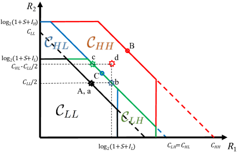
[$C_{LH}\leq C_{LL}/2+\log_{2}(1+S+I_{L})$] [$C_{LL}/2+\log_{2}(1+S+I_{L})<C_{LH}\leq 2\log_{2}(1+S+I_{L})$]
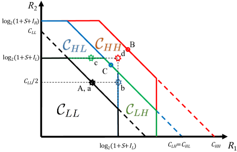
[$2\log_{2}(1+S+I_{L})<C_{LH}$]

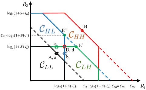
Figure 5: Capacity regions $\mathcal{C}_{xy}$ in (9) when the interference realizations are $I_{1}=I_{x}$ and $I_{2}=I_{y}$ if (a) $C_{LH}\leq C_{LL}/2+\log_{2}(1+S+I_{L})$; (b) $C_{LL}/2+\log_{2}(1+S+I_{L})<C_{LH}\leq 2\log_{2}(1+S+I_{L})$; and (c) $2\log_{2}(1+S+I_{L})<C_{LH}$. The points A, B, C, D, E, and E’ denote the rates selected by the RCC in the C-RAN scheme discussed in Sec. IV-A and the points a, b, c, and d indicate the four rate pairs $(R_{x},R_{y})$ selected by the F-RAN scheme in Sec. LABEL:Sec:F-RAN;Special.

An outage occurs at time $t$ if the selected rate pair $(R_{1},R_{2})$ is outside the capacity region $\mathcal{C}_{I_{1}(t)I_{2}(t)}$. Accordingly, the outage probability in a time slot $t$ for which the CSI available at the RCC is $I_{1}(t-d)=I_{1}$ and $I_{2}(t-d)=I_{2}$ can be computed as

$$\textrm{Pr}[(R_{1},R_{2})\notin\mathcal{C}({I_{1}(t),I_{2}(t)})|I_{1}(t-d)=I_{1},I_{2}(t-d)=I_{2}].$$ (10)

An achievable $\epsilon$-outage adaptive sum-rate is summarized in the next lemma, where we defined the probabilities $P_{xy}^{HH}=\beta^{H|x}(d)\beta^{H|y}(d)$, $P_{xy}^{LH}=\beta^{L|x}(d)\beta^{H|y}(d)$, $P_{xy}^{HL}=\beta^{H|x}(d)\beta^{L|y}(d)$, and $P_{xy}^{LL}=\beta^{L|x}(d)\beta^{L|y}(d)$. The notation $P_{xy}^{\bar{x}\bar{y}}$ indicates the probability of transitioning from delayed states $\{I_{1}(t-d)=I_{x},I_{2}(t-d)=I_{y}\}$ to current states $\{I_{1}(t)=I_{\bar{x}},I_{2}(t)=I_{\bar{y}}\}$.