Contribution to Viscosity from the Structural Relaxation via the Atomic Scale Green-Kubo Stress Correlation Function
Abstract
We studied the connection between the structural relaxation and viscosity for a binary model of repulsive particles in the supercooled liquid regime. The used approach is based on the decomposition of the macroscopic Green-Kubo stress correlation function into the correlation functions between the atomic level stresses. Previously we used the approach to study an iron-like single component system of particles. The role of vibrational motion has been addressed through the demonstration of the relationship between viscosity and the shear waves propagating over large distances. In our previous considerations, however, we did not discuss the role of the structural relaxation. Here we suggest that the contribution to viscosity from the structural relaxation can be taken into account through the consideration of the contribution from the atomic stress auto-correlation term only. This conclusion, however, does not mean that only the auto-correlation term represents the contribution to viscosity from the structural relaxation. Previously the role of the structural relaxation for viscosity has been addressed through the considerations of the transitions between inherent structures and within the mode-coupling theory by other authors. In the present work, we study the structural relaxation through the considerations of the parent liquid and the atomic level stress correlations in it. The comparison with the results obtained on the inherent structures also is made. Our current results suggest, as our previous observations, that in the supercooled liquid regime the vibrational contribution to viscosity extends over the times which are much larger than the Einstein’s vibrational period and much larger than the times which it takes for the shear waves to propagate over the model systems. Besides addressing the atomic level shear stress correlations, we also studied correlations between the atomic level pressure elements.
March 3, 2024
I Introduction
In simple considerations of supercooled liquids it is quite common to draw a parallel with the Maxwell viscoelastic model MaxwellJC18671 ; BlandDR19601 ; HansenJP20061 . In this model a spring and a viscous dump element are connected in series. If a strain is applied suddenly to the system then it instantly stretches or compresses the spring, storing the potential energy in it. The energy stored in the spring results in its tension or compression. Later, the energy stored in the spring is dissipated in the viscous dump element exponentially in time. In drawing the parallel with supercooled liquids it is assumed that a suddenly strained supercooled liquid stores in itself the potential energy due to elastic deformation and that later this elastically stored potential energy slowly dissipates through some microscopic processes that occur in the supercooled liquid. In the framework of this parallel, it is natural to assume that the elastic energy stored in the supercooled liquid should be associated with its stressed state.
In several recent publications it has been discussed that the inherent structures of the model liquids have non-zero macroscopic stress states HarrowellP20121 ; IlgP20151 ; HarrowellP20161 . It has been demonstrated that these non-zero stress states are related to the boundary conditions which put constraints on the allowable configurational states of the systems IlgP20151 . Given of the Maxwell model discussed above, it is natural to assume that the non-zero macroscopic stresses of the inherent states manifest about the potential energy elastically stored in the inherent states. Thus different inherent states should correspond to the different states of the elastic energy in nearly a tautological agreement with the definition of the inherent states. From this perspective transitions between the inherent states should be associated with dissipation or accumulation of the stored elastic energy.
Over the several decades the mechanism of the stress relaxation in supercooled liquids has been extensively discussed HansenJP20061 ; HarrowellP20121 ; IlgP20151 ; HarrowellP20161 ; McQuarrie19761 ; Green19541 ; Kubo19571 ; Helfand19601 ; Hoheisel19881 ; Woodcock19911 ; Woodcock20061 ; Steele19951 ; Picard20041 ; Leonforte20041 ; Tanguy20061 ; Tsamados20081 ; Leporini20121 ; Lemaitre20151 . Many of these considerations address stress relaxation through considerations of the stress correlations relevant to the Green-Kubo expression for viscosity HansenJP20061 ; HarrowellP20121 ; IlgP20151 ; HarrowellP20161 ; McQuarrie19761 ; Green19541 ; Kubo19571 ; Helfand19601 ; Hoheisel19881 ; Woodcock19911 ; Woodcock20061 ; Steele19951 ; Leporini20121 . In particular, it has been shown that in deeply supercooled liquids (parent liquids) relaxation of the Green-Kubo stress correlation function at large times corresponds to the relaxation of the Green-Kubo stress correlation function calculated on the inherent structures (i.e., on the structures obtained through “an instant quench” from the parent liquid structures) HarrowellP20121 ; IlgP20151 ; HarrowellP20161 ; Leporini20121 . Another direction in the considerations of the stress relaxation concerns the angular dependence of changes in the stress fields generated by local structural transformations Picard20041 ; Tanguy20061 ; Tsamados20081 ; Lemaitre20151 ; Chattorai20131 ; Puosi20161 .
In our previous considerations of the atomic stress correlations relevant to the Green-Kubo expression for viscosity we investigated the connection between viscosity and propagating shear stress waves Levashov20111 ; Levashov2013 ; Levashov20141 ; Levashov2014B . In particular, we found that the contribution to viscosity associated with the shear stress waves is very non-local in the model liquid even at temperatures well above the melting temperature. In those previous considerations the role of the structural relaxation in liquids has not been discussed Levashov20111 ; Levashov2013 ; Levashov20141 ; Levashov2014B . One (and, probably, the major) purpose of the current paper is to elucidate how the structural relaxation is expressed in the atomic stress correlation function. Previously the connection between the structural relaxation and viscosity has been addressed from the perspective of the inherent structures Leporini20121 ; HarrowellP20121 ; HarrowellP20161 . Here we suggest that the structural relaxation in the Green-Kubo stress correlation function of a parent liquid at times larger than few Einstein’s vibrational periods can essentially be taken into account through the consideration of the atomic stress autocorrelation term only. Another purpose of the paper is to assess the generality of the previously obtained results through consideration of a different system. The binary model system that we consider in this paper can be supercooled to significantly lower temperatures than the single component system that has been studied in Ref.Levashov20111 ; Levashov2013 ; Levashov20141 ; Levashov2014B . Finally, we studied the atomic scale pressure-pressure correlation function. Behavior of this correlation has not been studied previously from the perspective of the atomic scale correlations. We found that the pressure-pressure correlations (longitudinal waves) are very well pronounced in the atomic scale pressure-pressure correlation function.
Our current interpretations of the results are strongly influenced by Ref.Petravic20051 . In Ref.Petravic20051 the vibrational contribution to the crystals’ viscosity has been considered. It has also been stated there that situation in supercooled liquids is different in a sense that there is an additional contribution to the liquids viscosity from the structural relaxation. While these results at present appear to be quite natural, we mention them because in Ref.Petravic20051 the vibrational contribution to viscosity has been explicitly and carefully discussed. Those discussions appear to be well aligned with our previous and the current results. For our purposes, we interpret the results of Ref.Petravic20051 in the following way. We assume that if (while) a supercooled liquid remains trapped in an inherent state for some (long) time then during this time there is essentially only the vibrational contribution to viscosity. Transitions between the inherent states represent the contribution to viscosity associated with the structural relaxation. In this paper we address how the structural relaxation is reflected in the atomic stress correlation functions. The role of the structural relaxation with respect to viscosity has also been addressed in recent Ref.Leporini20121 ; HarrowellP20121 ; HarrowellP20161 . It is of interest that our present results suggest a picture that is noticeably simpler than some of the conclusions presented in Ref.HarrowellP20161 . In Ref.HarrowellP20161 it has been concluded that there is structural contribution to viscosity associated with the large distances. See Fig.6,7,8,9 of Ref.HarrowellP20161 . Our results suggest that one can account for the contribution to viscosity from the structural relaxation essentially through the consideration of the atomic level stress autocorrelation function, i.e., through the zero-distance contribution. This interpretation does not imply that there is only zero distance contribution to viscosity from the stress relaxation. This result occurs because large distances cause alternating positive and negative contributions to viscosity which cancel each other.
The paper is organized as follows. In section II we describe the approach used to study the stress correlations. In section III we describe the model system that has been used in our simulations. In section IV we describe and discuss the obtained results. In the discussion section V we briefly address the connection between our results and the results obtained previously within the mode-coupling theory approaches. We conclude in section VI.
II Vibrational and Structural Contributions to Viscosity
II.1 Expansion of the macroscopic Grenn-Kubo stress correlation function in terms of the atomic level stresses
The starting point for the used approach is the well-known Green-Kubo expression for (zero-wavevector and zero-frequency) viscosity HansenJP20061 ; Green19541 ; Kubo19571 ; Helfand19601 ; Hoheisel19881 :
| (1) |
where is the volume of the system, is the Boltzmann constant, is the temperature, is the component of the macroscopic stress tensor of the sample. The averaging if done over the equilibrium canonical ensemble (in practice, over the initial times, , under the assumption that ergodicity holds).
It has been discussed in Ref.Erpenbeck19951 that the derivations of (1) have been done for the systems of infinite size without any assumptions with respect to the applied periodic boundary conditions. However, Eq.1 is routinely used in MD simulations with the Periodic Boundary Conditions (PBC) applied. It follows from Ref.Erpenbeck19951 and also from our previous investigations that the effects of the PBC are far from being trivial Levashov20111 ; Levashov2013 ; Levashov20141 ; Levashov2014B . This issue will arise again in this paper.
Further we assume that interactions between the particles can be described by pair potentials. We also assume that contributions to the stress tensor from the terms associated with the particles’ velocities can be neglected, as they are usually small in dense supercooled liquids in comparison to the contributions from the terms associated with interactions between the particles Hoheisel19881 . In this case, the expression for the macroscopic stress tensor, , can be written as: HarrowellP20121 ; IlgP20151 ; HarrowellP20161 ; McQuarrie19761 ; HansenJP20061 ; Green19541 ; Kubo19571 ; Helfand19601 ; Hoheisel19881 ; Woodcock19911 ; Woodcock20061 ; Levashov20111 ; Levashov2013 :
| (2) |
where is the number density of the particles, and . In the following, we refer to the quantities as to the local atomic stress elements. We note that the local atomic stress elements differ from the local atomic stresses because there is no local atomic volume present in their definitions Egami19801 ; Egami19802 ; Egami19821 ; Chen19881 .
Using the first expression from (2), expression (1) can be rewritten as:
| (3) |
where
| (4) | |||
| (5) |
and
| (6) | |||
| (7) |
In (7) and -is the delta function. In treating the data from computer simulations, summation in (7) is assumed to be over those particles that are within some narrow interval of distances from the position of at time .
As far as we know, the expansion of (1) into expressions (4,5,6,7) at first has been done in Ref. Woodcock19911 ; Woodcock20061 . In our view, this expansion provides a natural view on the atomic scale stress correlations that determine viscosity. Correlations between the atomic scale stresses have been considered by several authors in the contexts of the stress relaxation and angular dependent stress fields. HarrowellP20161 ; Voigtmann2016 ; Leporini20121 ; Lemaitre20151 ; Chattorai20131 ; Puosi20161 ; Levashov20111 ; Levashov2013 ; Levashov20141 ; Levashov2014B ; Levashov20162 .
In the calculations the results of which we present in the following we used a further development in the interpretations of Eq.(6,7). In particular, in order to calculate the stress correlation functions in Eq.(6,7) we used expressions (51,52,53,54) from Ref. Levashov20162 . This approach automatically performs the averaging over the equivalent stress correlation functions, such as , , and . In any case, for the purposes of this paper, one can simply assume that calculations have been done according to the Eq.(6,7).
II.2 Correlations between the atomic level pressure elements
Besides considering correlations between the atomic level shear stress elements, we also present results for the correlations between the atomic level pressure elements. The atomic pressure element on every particle is defined as:
| (8) |
The average value of the atomic pressure, in general, is not equal to zero and can be calculated as:
| (9) |
where the “X” subscript is “A” or “B” depending on the type of the particle . We calculated the average values of the pressure for the particles of type “A” and the particles of type “B” separately. It is known that the average values of the pressure elements on the particles of different types are different Levashov20162 ; Aur19871 . If the average value of the atomic scale pressure is averaged over all particles in the system, irrespective of their types, then this value corresponds to the macroscopic value of the pressure. In performing the calculations, we calculated the average value of the pressure for every time frame, i.e., we did not use the value of the pressure averaged over the different time frame. Thus there is an additional difference with the calculations done for the atomic scale shear stress correlation functions – in those calculations we assume that the average value of every atomic scale shear stress component is zero. For deeply supercooled liquids this issue is a delicate one because deeply supercooled liquids can be trapped for a long time in the states with non-zero macroscopic shear stress HarrowellP20121 ; IlgP20151 ; HarrowellP20161 ; Petravic20051 .
In order to define the pressure-pressure correlation function we introduce the following notation:
| (10) |
where the average value is calculated on the same sample at time , i.e., on the same sample on which is calculated.
We calculated the correlation function between the atomic level pressure elements according to:
| (11) |
In (11) the averaging is done over the pairs of particles of the proper types and over the initial, (), time frames.
II.3 Correlations between the stress changes of different particles
Before proceeding further, it is worth noting that the stress correlation functions introduced above are closely related to the correlation functions between the particles’ stress changes. This observation has also been pointed out in Ref.Lemaitre20151 . Indeed, let us consider the following correlation function:
| (12) |
where
| (13) |
Thus correlation function (12) addresses correlations in the changes of stresses of particles separated at time by distance . The expression (12) can be rewritten as:
| (14) |
where
| (15) | |||
| (16) | |||
| (17) |
Note in (16) that the values of the stresses are evaluated at time , while the -function is calculated at time . Let us assume that we consider a deeply supercooled liquid and such times during which the positions of the particles do not change significantly (no particles’ jumps occur). In this situation it is reasonable to expect that: . Under this assumption, it follows from Eq.7 that if then it is reasonable to expect that:
| (18) |
II.4 Structural and vibrational contributions to the particles’ stress elements and to the stress correlation function.
It has been discussed in Ref.HarrowellP20121 ; IlgP20151 ; HarrowellP20161 that the inherent states, obtained from the parent liquid at some temperature through the steepest descent or conjugate gradient relaxations, possess non-zero macroscopic stresses. The considerations in Ref.HarrowellP20121 ; IlgP20151 ; HarrowellP20161 are relevant for the finite size systems under the periodic boundary conditions. However, the Green-Kubo expression for viscosity has been derived under the assumption that the system is of infinite (macroscopic) size. This issue has been described in some details in Ref.Erpenbeck19951 . Actually, in our view, in the originally derived expression the concept of the macroscopic stress is simply absent. It is, of course, natural to define the macroscopic stress tensor through the atomic scale interactions. However, in our view, the expressions derived originally essentially consider the atomic scale stress correlation functions. Indeed, according to expressions (6,7), it is reasonable to think about the macroscopic viscosity as about the quantity whose value is determined by the microscopic (atomic scale) correlation. We adopt this point of view in our considerations. In this context, we note that it is unclear how to define the macroscopic inherent structure stress for an infinite-size system. For this reason we consider the structural and vibrational contributions to the atomic stresses and their correlations without making a reference to the macroscopic stresses associated with the inherent structures.
Some additional considerations with respect to the macroscopic inherent stresses for the finite size systems are given in subsection (IV.7).
II.5 A consideration for the system of infinite size
Let us assume that we consider a system of infinite size. Further we assume that the value of the atomic stress tensor of a particle is formed by the structural and vibrational contributions:
| (19) |
It is possible to think about the structural contribution to the atomic stresses, , as about the stresses on the atoms in the corresponding inherent structures. Using (1,2,19) and the assumptions of time-translational invariance and reversibility we express the macroscopic stress correlation function through the atomic stress correlations:
| (23) | |||||
In order to proceed further we assume that there are no correlations between the structural and vibrational contributions to the atomic stresses. Under this assumption the term (23) is equal to zero.
If the term (23) is equal to zero then the expression above suggest that it can be assumed that there are two contributions to viscosity; one contribution (23) is associated with the structural correlations (structural relaxation), while another (23) with the vibrational correlations (vibrational relaxation).
It follows from our previous publications Levashov20111 ; Levashov2013 ; Levashov20141 ; Levashov2014B and the data presented in this paper that the vibrational relaxation can be interpreted as originating from the decay of the propagating stress waves. It has also been briefly discussed in Ref.Levashov20141 that the structural stress relaxation should be related to the decay of the van Hove correlation function.
In the present paper we show that the contribution to viscosity from the structural relaxation can be accounted for through the consideration of the atomic stress auto-correlation term (4). This does not mean that there are no structural contributions to viscosity from the larger distances. This situation arises because the long-range structural correlations carry positive and negative contributions to viscosity and thus the long-range structural contributions to viscosity effectively cancel each other.
III The Model
We studied a binary equimolar system of particles in 3D interacting through purely repulsive potential(s):
| (24) |
where the notations “” and “” stand for the types of particles: “” or “”. The used values of the parameters are: , , . The large -particles have masses which are two times larger than the masses of the small -particles: . The chosen value of the particles’ number density was: .
In the following we measure the distances in the units of and the temperature in the units of . The unit of time that arises from the model’s parameters is . In the following we measure time in the units of .
The model that we used in our simulations has been extensively studied previously Hansen19881 ; Miyagawa19911 ; Mizuno20101 ; Mizuno20111 ; Matsuoka2012 ; Mizuno20131 . The freezing point of the corresponding one-component system is approximately Miyagawa19911 . At the system is in a deeply supercooled state Mizuno20101 ; Mizuno20111 ; Matsuoka2012 ; Mizuno20131 . In Ref.Levashov20162 we studied instantaneous properties of the atomic stresses and stress correlations in the described model.
Molecular Dynamics simulations have been performed with the LAMMPS program Plimpton1995 ; lammps . The typical value of the time step used was . The relaxations of the parent liquid structures into the inherent states have been performed with the conjugate gradient method within the LAMMPS program.
IV Results
IV.1 The studied temperatures and the relevant timescales
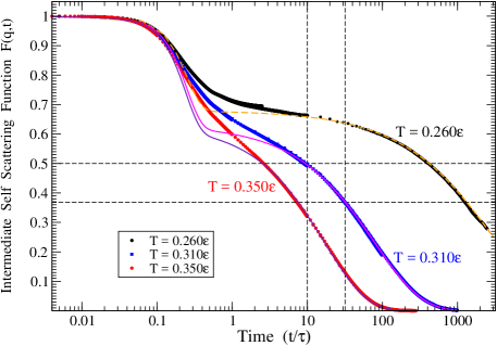
In this paper we present the results for the temperatures , , and . The temperature corresponds to the beginning of the true supercooled liquid regime, while the temperature is well in the supercooled region Hansen19881 ; Miyagawa19911 ; Mizuno20101 ; Mizuno20111 ; Matsuoka2012 ; Mizuno20131 . In order to provide more intuitive insights into these temperatures we show in Fig.1 the intermediate self scattering functions for the small “A” particles at these temperatures. More detailed information concerning the timescales of the studied model can be gained from Ref.Hansen19881 ; Miyagawa19911 ; Mizuno20101 ; Mizuno20111 ; Matsuoka2012 ; Mizuno20131 .
IV.2 The macroscopic shear stress correlation function
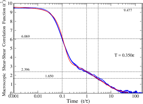
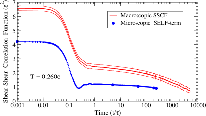
The macroscopic shear stress correlation function for is shown in Fig.2. The comparison of Fig.2 with Fig.1 demonstrates that the shear stress correlation function decays noticeably faster than the intermediate self scattering function. This result also follows from the comparison of the timescales obtained from the fits of the curves in these figures with the compressed and stretched exponential functions. Thus, for temperature the time relevant to the long-time decay of the intermediate self-scattering function is , while the time relevant to the long time behavior of the shear stress correlation function is almost 6 times smaller, i.e., . Note, however, that the fitting functions used for the two curves are different. The different time dependencies of the intermediate self-scattering function and the macroscopic stress correlation function can be understood on the basis of the mode-coupling theory (MCT) Balucani19881 ; Balucani19901 ; Gotze1998sw . From Fig.2 it is quite clear that the time corresponds to the Einstein’s vibrational period HansenJP20061 .
In the following we are going to show that in the time interval between and there is a significant contribution to the shear stress correlation function associated with the propagating shear waves.
IV.3 The microscopic (atomic scale) shear-shear and pressure-pressure correlation functions
For the calculations of the stress correlation functions, we had chosen the value of the bin size because it provides good resolution of the first peak in the correlation functions. For the distances beyond , the values of the stress correlation functions for every value of were obtained by averaging over the values of the stress correlation function at the nearest points (five points from the left, the point itself, and five points from the right). This procedure reduces the noise at large distances without affecting the actual behavior of the averaged stress correlation curves. For the distances the averaging procedure over the values has not been used.
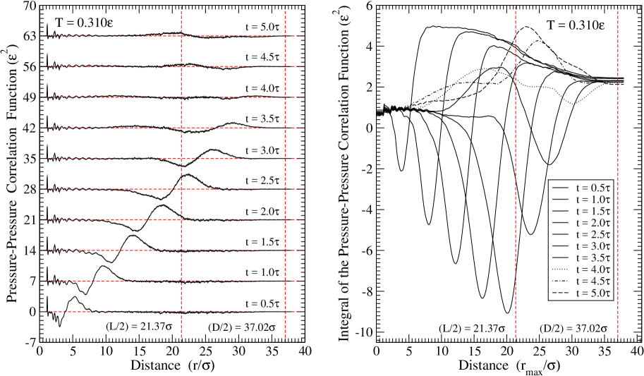
Figure 3 shows the microscopic Shear-Shear Correlation Functions (SSCF ) and the microscopic Pressure-Pressure Correlation Functions (PPCF ) calculated according to the formulas (4,5,6,7) and (8,9,10,11). In order to obtain these correlation functions the particles coordinates were saved with time interval . Then the correlation functions for particular times were calculated using the saved particles’ coordinates. Thus, at first, the stress correlations functions for particular times were calculated as the functions of distance and then the results for the different times we combined to produce Fig.3. Note that the actual time interval between the time values presented in Fig.3 is .
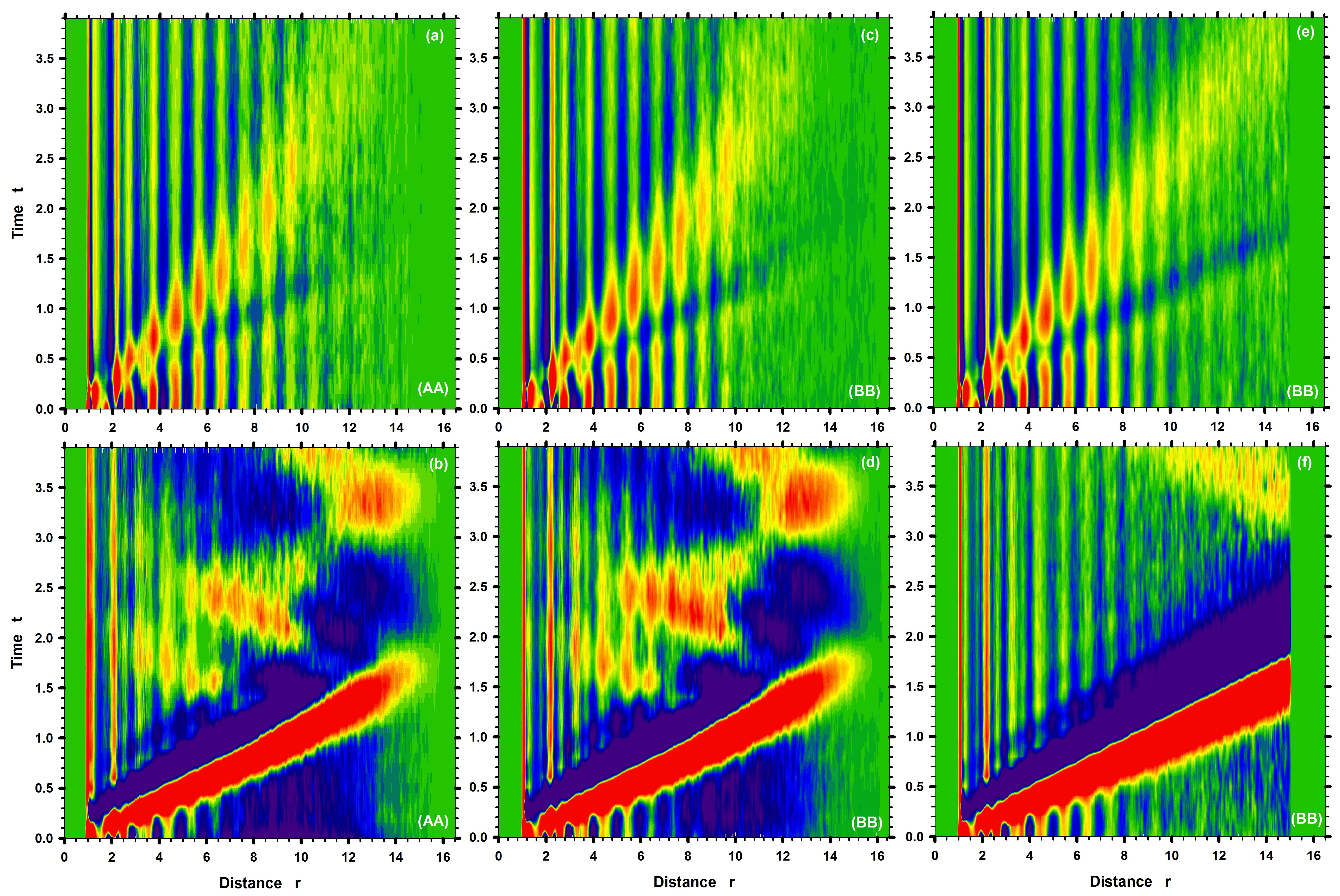
The similar shear-shear correlation functions have been obtained previously for a different single component system of particles in Ref.Levashov20111 ; Levashov2013 ; Levashov20141 . The results presented in Fig.3 establish the generality of the previously obtained results. The shown pressure-pressure correlation functions have not been calculated previously.
The results presented Fig.3 give an impression that the central particle at time zero emits the shear and compression waves that propagate away from the central particle as time increases. This interpretation is reminiscent of the Huygens-Fresnel principle in optics. In Ref.Levashov2014B we have shown that a picture qualitatively similar to the one presented in Fig.3 can be obtained through the consideration of the plane wave vibrations (phonons) in a model crystal. Thus, while it is possible to assume that every particle in a liquid is a source of the stress waves at every instant, it is also possible to assume that the stress correlations shown in Fig.3 arise from non-local vibrations.
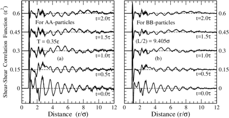
I order to provide further insight into the data presented in Fig.3 we show in Fig.4 the microscopic shear-shear correlation functions calculated for some particular times, i.e., for the constant time cuts of the stress correlation functions presented in Fig.3. The Fig.4(a) shows the shear-shear correlation functions between the particles of type “A”, while the Fig.4(b) shows the shear-shear correlation functions between the particles of type “B”. Note the positions and the relative intensities of the shear-shear waves in the shown curves. The curves presented in Fig.4(a,b) were not normalized to the intensity of the first peak associated with the first nearest neighbors, while the data in Fig.3 were normalized.
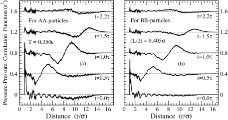
The constant time cuts of the pressure-pressure correlation functions presented in Fig.3(b,d) are shown in Fig.5(a,b). From the comparison of Fig.5 with Fig.4 we again can conclude that the pressure-pressure waves are more pronounced than the shear-shear waves. Of particular interest is the negative intensity in the pressure-pressure correlation function at in the interval of distances . In our view, the region can be associated with the pressure correlation range for the pressure-pressure correlations. Let us now consider the curves corresponding to . These curves exhibit positive intensities in the region . From the comparison with Fig.3(b,d) it follows that this positive intensity arises due to the pressure-pressure waves that “left” and “reentered” the simulation box.
IV.4 Integral over distance of the microscopic shear-shear correlation function
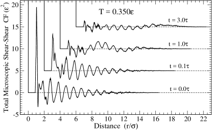
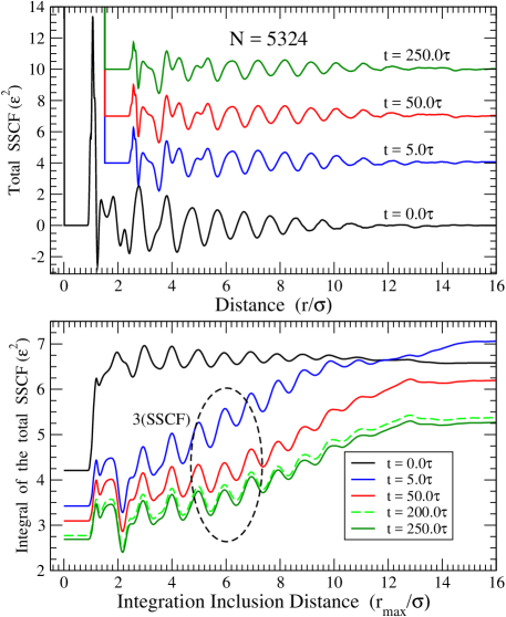
The partial microscopic SSCFs for the “AA”, “AB”, “BA”, and “BB” particles can be summed up to produce the total microscopic SSCF . These total microscopic SSCFs for the selected times are shown in Fig.6. The selected times in Fig.6 are the same as the selected times in Fig.2. According to the definition of the microscopic SSCF (4,5,6,7), the integrals over the distance of the SSCFs shown in Fig.6 should be equal to the values of the macroscopic SSCF in Fig.2 at the corresponding times.
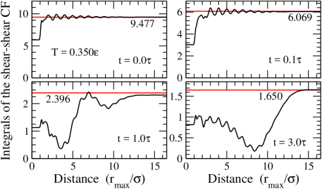
Figure 7 shows how the integrals of the microscopic SSCF (black curves) converge to the macroscopic SSCF (red horizontal lines) as the upper integration limit, , increases. The convergence of the black curves to the red horizontal lines, as all distances become included, elucidates the role of the shear stress waves and large distances in the formation of viscosity.
Note in Fig.7 that the shown black curves have non-zero values at zero distances. These non-zero values originate from the stress auto correlation term (4,6). Then at times and there are rises in the values of the integrals associated with the inclusion of the first nearest neighbors. It is of interest that at times and it is less clear if there are contributions associated with the first nearest-neighbor shell. In any case, they appear relatively smaller than the contributions from the first nearest neighbors at the times and . Moreover, it appears that some parts of the contribution associated with the first nearest neighbors at small times become associated with the shear waves at later times. Note, for the time , that the minimum at originates from the footprint of the pressure-pressure wave, as can be recognized from the behavior of the shear stress correlation function in Fig.3(a) at .
IV.5 Structural contribution to the microscopic stress correlation functions
In our previous considerations of the microscopic SSCFs the connection between the propagating shear waves and viscosity has been discussed Levashov20111 ; Levashov2013 ; Levashov20141 ; Levashov2014B . However, the connection between viscosity and the structural relaxation has not been addressed. The role of the structural relaxation becomes especially relevant in considerations of supercooled liquids. It has been demonstrated that structural relaxation in supercooled liquids proceeds via the localized rearrangement events Picard20041 ; Leonforte20041 ; Tanguy20061 ; Tsamados20081 ; Leporini20121 ; Chattorai20131 ; Chandler20111 . Thus there arises a question: “How these local rearrangement events are expressed in the microscopic SSCFs and how do they contribute to viscosity?”
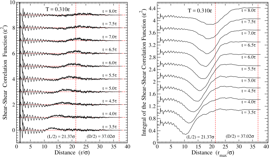
In our discussion of Fig.7 we noticed that there is a contribution to viscosity associated with the autocorrelation term in the SSCFs . In the following, we suggest that the structural contribution to viscosity at large times can be taken into account through the consideration of this autocorrelation term. In order to demonstrate this, we performed calculations of the microscopic SSCF for the large times up to the distances that allow to include all particles in the large system. Thus, we considered the system of particles with (i.e., ). We studied this system at . We saved the particles coordinates every and then used these coordinates to calculate the shear-shear and the pressure-pressure correlation functions. The results for the selected large times are shown in Fig.8,9.
In the left panel of Fig.8 we see that for the time the shear stress wave has not yet reached the distance . Thus the positive peak of the shear stress wave is located at , (“the center” of the wave, according to Ref.Levashov2014B , is actually located at , i.e., at the point where the SSCF crosses the time axis.) The curves corresponding to the times , , , and represent the situation when some parts of the “shear waves” have already left the simulation box at . Note, however, that after reentering the simulation box, these shear waves have not yet reached the distance . This can be seen from how the shear stress waves disappear as they move further along the main diagonal beyond . Thus, for the shear wave has not yet reached the distance . This also means that the part of the wave that reentered the box has not yet reached the distance . Further note that, besides the oscillations, the region of distances between and is essentially flat. In our view, this region at the times , , , represents the general behavior of the “behind the wave region” that one should observe in the system of infinite size. In our view, the presented results suggest that in the system of infinite size the ”behind the wave region” should be essentially flat, if the oscillations are ignored. Note also that the amplitudes and the shapes of the oscillations in the region between and are quite similar in all curves. The change in these oscillations can be considered as an intuitive measure of the structural relaxation. It follows, from this perspective, that there occur only some moderate structural relaxation as time increases from to .
Let us now consider the curves in the right panel of Fig.8.
These curves show how the integrals of the curves from the left panel depend
on the upper integration limit .
There are four points with respect to the curves in the right panel that we would like to note.
1) The values of the curves at are not zero.
These non-zero values are due to the contributions from the shear-shear
autocorrelation term (6) that has been taken into account.
2) There is essentially a flat region between and for the curves corresponding
to the times , , , and .
It is quite clear, in our view, that the small decreases in the values of these integral
curves around are due to the negative tails of the propagating shear waves.
3) As the distance increases beyond there is, at first, the negative contribution
to integral curves from the “negative tails” of the shear waves and then there
is a positive contribution from the “positive fronts” of the shear waves.
The overall contributions of the shear waves to the integral curves are positive.
4) Finally, note that there are only small changes in the shape and
the amplitude of the peak originating from the nearest neighbor shell, i.e., in
the peak located at in all curves.
This means that for all considered times the contribution to viscosity
from the nearest neighbor shell is approximately the same.
Thus, it is quite natural to expect that for the considered times
the contributions to viscosity from the autocorrelation
term (i.e., from the -peak) are not very different.
The left panel of Fig.9 shows the microscopic PPCFs at large times. Note that there, as in the left panel of Fig.8, are essentially flat behind the wave regions (besides the structural oscillations). Thus we come to the conclusion that the structural contribution to the macroscopic PPCF (i.e., to the integral over the distance of the microscopic PPCF ) can be estimated through the consideration of the microscopic pressure-pressure auto-correlation term only. Thus the situation with the PPCF is similar to the situation with the SSCF . The right panel of Fig.9 shows the integrals over the distance of the curves shown in the left panel. This time we did not shift the curves vertically, in contrast to the integral curves in Fig.8. Note that all curves have almost the same value at zero distances. Thus for the discussed times the pressure-pressure auto-correlation term changes only a little. This means, according to our interpretation of these changes as being related to the structural relaxation, that structural relaxation proceeds quite slowly. It is more surprising that the integral curves, after the integration over all distances, again converge to almost the same value. It means that the vibrational contributions to the integral curves at the considered times are somewhat similar. We speculate on the origin of this behavior from the perspective of dissipation of the pressure waves, i.e., we assume that the waves’ contribution to the integral curves is related to the loss of intensity of the pressure waves. In our view, it can be assumed that the pressure wave is already “formed” at . Further, it can be assumed that the rate of dissipation of the pressure wave so small that the overall intensity of the pressure wave does not change significantly over the time interval . On the other hand, it is natural to assume that the rate of the energy loss of the pressure wave is proportional to the energy of the pressure wave. Thus, it appears that the data suggest that the energy of the wave for the discusses times decay exponentially in time with a rather large dissipation time : , where is the energy of the pressure wave at .
The given above description of the obtain data leads us to the following conclusions. It is possible to speak about the vibrational and the structural contributions to viscosity. The vibrational contribution originates from the propagating shear waves. The value of the structural contribution is essentially determined by the contribution that comes from the shear stress autocorrelation term (4,6) (and a small addition from the first peak in the shear-shear correlation function). The region of distances beyond the first nearest neighbors contains alternating positive and negative structural contributions to viscosity. These positive and negative structural contributions from the large distances mutually cancel each other. This cancellation leads to the situation in which the structural contribution to viscosity can be accounted through the consideration of the stress autocorrelation term and a small contribution associated with the first peak in the shear stress correlation function.
IV.6 Results for larger times
In view of the results presented in Fig.8,9, it is reasonable to consider also the behavior of the microscopic SSCF at the times much larger than the time required for the shear waves to propagate through the system. In particular, compare the contribution to the macroscopic SSCF from the autocorrelation stress term with the contribution from the propagating shear waves. The results of the relevant calculations for the system with are shown in Fig.10,11(a,b) for which is deeper in the supercooled region than the temperatures considered before.
The thick red curve in Fig.10 shows the dependence of the macroscopic SSCF on time for . The blue curve in Fig.10 shows the contribution to the macroscopic SSCF associated with the autocorrelation self-term. It is natural to associate the difference between the red and blue curves with the non-local contribution which should be related to the shear stress waves.
Figure Fig.11(a) shows the total microscopic shear stress correlation functions at the selected times, while Fig.11(b) shows the integrals over the distance of the curves shown in Fig.11(a).
In agreement with Fig.10, it follows from Fig.11(b) that at large times there is the contribution to viscosity associated with the distances beyond the first neighbors.
In view of the results presented before, it is quite natural to associate this long-range contribution with the shear stress waves that passed many times through the system and which are essentially distributed over the whole finite-size simulation box. In other words, it means that the positive and homogeneous contribution from the large distances is a finite size effect, i.e., if the system were of infinite size then there would be instead the contribution from the very large distances corresponding to the position of the shear wave.
IV.7 Microscopic SSCF from the inherent structures
In Ref.HarrowellP20161 the microscopic SSCFs calculated on the inherent structures have been considered. It is natural to expect that relaxation into the inherent states removes the vibrational contributions to the atomic stresses and, as a consequence, to the SSCFs and to the integrals over the stress correlation functions. However, the results obtained in Ref.HarrowellP20161 show that there is a positive contribution to the integral of the SSCF associated with the distances beyond the first neighbors.
To understand the origin of this situation we also produced the inherent structures from the parent liquid at and calculated the microscopic SSCFs on these structures. The inherent structures were produced by the conjugate gradient minimization procedure within the LAMMPS program. We performed calculations of the inherent microscopic SSCFs on the systems with and . Figure 12(a) shows that the results for the SSCFs obtained on two systems look rather similar. However, the small differences between the SSCFs lead to the noticeable differences between the integrals of these SSCFs over the distances, as Fig.12(b) shows.
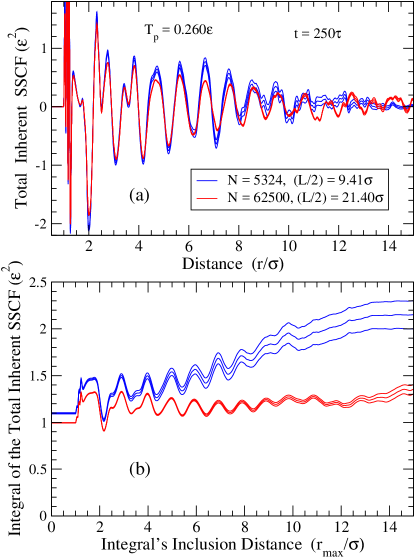
In our view, the different behaviors of the integrals of the SSCFs at large distances are caused by the different values of the fluctuations of the macroscopic inherent structure stresses, as discussed below.
At first, we introduce several notations. We assume that the atomic level stress element of a particle in an inherent configuration, , can be decomposed into the two parts:
| (25) |
where the macroscopic inherent structure stress, , and the atomic structural stress, , are defined as:
| (26) | |||
| (27) |
According to Ref.HarrowellP20121 ; IlgP20151 ; HarrowellP20161 , the macroscopic inherent stress, , in general, is not equal to zero.
In calculations of the microscopic stress correlation functions we consider the correlations between the inherent stress elements of particle , , with the inherent stress elements of those particles , , which are distance away from the particle at time :
| (28) | |||
| (29) | |||
| (30) | |||
| (31) | |||
| (32) |
The expression above can be simplified if several assumptions are made. In particular, in our view, it is reasonable to assume that there is no correlation between the structural atomic stress and the average macroscopic inherent stress. This is essentially the consequence of the definitions (26,27). Thus (30) and (31) are equal to zero. It is also reasonable to assume that there is a positive correlation between the average inherent stresses at times and . Under this assumption the contribution from (29) grows with the increase of . The smaller is the size of the system the larger are fluctuations in the values of the average inherent stresses. Thus, it is naturally to expect that the value of the term (29) increases as system’s size decreases. In our view, this might be the explanation of the large-distance contribution to the integral of the microscopic stress correlation function calculated on the inherent structures.
V Discussion
In view of the author, the major result of this paper is the realization that the atomic scale stress correlation function, discussed previously in Ref.Levashov20111 ; Levashov2013 ; Levashov2014B ; Levashov20141 , contains in itself not only the vibration contribution to viscosity, as it has been assumed, but also the contribution from the structural relaxation.
We note that in some recent papers importance of the propagating stress waves for the glass transition has been discussed Trachenko20091 ; Trachenko20161 . Correlations between the local rearrangement events and viscosity also have been addessed Iwashita20131 ; Ashwin20151 .
The interpretations suggested here appears to be well aligned with the philosophy behind the mode-coupling theory (MCT) where it is assumed that the memory functions related to the evolutions of the correlations functions can be split into the rapidly decaying binary collision part and a slowly decaying mode-coupling part that couples the decay of the considered correlation functions to the density fluctuations, i.e., to the static structure factor and to the intermediate scattering function(s) Gotze19841 ; Leutheusser19841 ; Kirkpatrick19841 ; Kirkpatrick19861 ; Marchetti19921 ; Balucani19871 ; Balucani19881 ; Gotze1998sw ; Balucani19901 ; Marchetti19921 ; Balucani19931 ; Balucani1994book ; Balucani2001 ; Das20021 ; Egorov20081 ; Bryk20161 ; Gonzales20171 .With respect to the transverse current correlation function and the macroscopic Green-Kubo stress correlation function, this approach has been described in Ref. Kirkpatrick19841 ; Kirkpatrick19861 ; Marchetti19921 ; Balucani19871 ; Balucani19881 ; Gotze1998sw ; Balucani19901 ; Marchetti19921 ; Balucani19931 ; Balucani1994book ; Balucani2001 ; Das20021 ; Egorov20081 ; Bryk20161 ; Gonzales20171 . In particular, it allows obtaining a very good fit of the simulated macroscopic stress correlation functions for alkali metals near the melting point with the curves calculated within the MCT approach Balucani19931 . At present, various issues related to this approach are still discussed in the literature Balucani2001 ; Das20021 ; Egorov20081 ; Bryk20161 ; Trachenko20161 ; Gonzales20171 .
In our view, the data presented here might offer some additional insight into the nature of the mode-coupling memory term discussed in the MCT approach. In particular, the data presented in Fig.1,2 suggest that the binary collision term should not be of importance for the times larger than . Further, the results suggest that for the times the stress correlation functions are still formed by two distinct contributions. One contribution can be associated with the propagating longitudinal and shear waves while another contribution is associated with the structural relaxation Gotze1998sw . From this perspective, it is of interest to develop a better understanding of how these features are related to the features of the mode-coupling memory term or to the van Hove correlation function. Ideally, it is desirable to have the MCT predictions for the behaviors of the atomic scale stress correlation functions.
From the perspective of the potential energy landscape (PEL) approach, our results suggest the presence of non-trivial size effects in the stress correlation functions calculated on the inherent structures. This issue requires further investigations.
VI Conclusion
We investigated the behavior of a binary system of repulsive particles from the perspective of the atomic scale stress correlation functions that are directly relevant to the Green-Kubo expression for viscosity. In this paper, we studied the behavior of the stress correlation functions at the temperatures which are deeper in the supercooled liquid range than the temperatures that we studied previously for the single component systems.
The major result of this paper is the elucidation of the contribution from the structural relaxation to the atomic scale stress correlation functions relevant for the Green-Kubo expression for viscosity. Analysis of the results shows that the contribution from the structural relaxation to viscosity can be accounted through the consideration of the atomic stress autocorrelation function (there is also a relatively small contribution associated with the nearest neighbor shell). However, this does not mean, in our view, that viscosity is a local quantity from the perspective of the structural relaxation. The situation that it is sufficient to consider only the contributions from the stress autocorrelation function and the nearest neighbor shell arises because positive and negative contributions from the larger distances mutually cancel each other.
Besides the contribution to viscosity associated with the structural relaxation there is also the contribution associated with the shear waves Levashov20111 ; Levashov2013 ; Levashov20141 . The results presented here demonstrate the generality of the results obtained previously for a single component system Levashov20111 ; Levashov2013 ; Levashov20141 . In particular, we again observed the shear waves propagating over the large distances and demonstrated their relation to viscosity. We found that the contribution from the shear waves can be observed for the times which are much larger than it takes for the stress waves to propagate through the system. The results also show the important role of the periodic boundary conditions for understanding the structure of the stress correlation functions.
In comparison to the previous publications, we also studied the propagation of the atomic scale pressure-pressure correlation waves. It was found that the pressure-pressure correlation waves are much more pronounced than the shear-shear correlation waves. The obtained results also show that the attenuation of the pressure waves is less significant than the attenuation of the shear waves. Besides, the results suggest that there might exist a structural pressure-pressure correlation range. This issue requires, in our view, further investigations.
Analysis of the stress correlation functions calculated on the inherent structures of different sizes suggests the presence on non-trivial size effects in the considered correlation functions. This issue also requires further considerations.
VII Acknowledgments
We are grateful to the second referee of this paper for bringing to our attention several highly relevant papers on the Mode-Coupling Theory.
We are grateful to the Supercomputing Center of the Novosibirsk State University for provided computational resources.
References
- (1) J. C. Maxwell, On the Dynamical Theory of Gases, Phil. Trans. R. Soc. Lond., 157, 49-88, (1867).
- (2) D. R. Bland, The Theory of Linear Viscoelasticity, (Pergamon Press, Oxford, 1960).
- (3) J. P. Hansen and I. R. McDonald, Theory of Simple Liquids, (3rd ed., Academic Press, London, 2006).
- (4) S. Abraham and P. Harrowell, The origin of persistent shear stress in supercooled liquids, J. Chem. Phys. 137, 014506 (2012).
- (5) I. Fuereder and P. Ilg, Influence of inherent structure shear stress of supercooled liquids on their shear moduli, J. Chem. Phys. 142, 144505 (2015).
- (6) S. Chowdhury, S. Abraham, T. Hudson, and P Harrowell, Long range stress correlations in the inherent structures of liquids at rest, J. Chem. Phys. 144, 124508 (2016).
- (7) D. A. McQuarrie, Statistical Mechanics, (Harper & Row, New York, 1976), Chap. 21.
- (8) , M.S. Green, Markoff random processes and the statistical mechanics of time-dependent phenomena. II. Irreversible processes in fluids, J. Chem. Phys. 22, 398 (1954).
- (9) R. Kubo, Statistical-Mechanical Theory of Irreversible Processes. I. General Theory and Simple Applications to Magnetic and Conduction Problems, J. Phys. Soc. Jpn. 12, 570 (1957).
- (10) E. Helfand, Transport Coefficients from Dissipation in a Canonical Ensemble, Phys. Rev. 119, 1 (1960).
- (11) C. Hoheisel and R. Vogelsang, Thermal transport coefficients for one and two-component liquids from time correlation functions computed by molecular dynamics, Comput. Phys. Rep. 8, 1 (1988).
- (12) S. Sharma and L.V. Woodcock, Interfacial Viscosities via Stress Autocorrelation Functions, J. Chem. Soc. Faraday Trans., 87(13), 2023-2030 (1991).
- (13) L. V. Woodcock, Equation of State for the Viscosity of Lennard-Jones Fluids, AIChE J. 52(2), 438 (2006).
- (14) H. Stassen and W.A. Steele, Simulation studies of shear viscosity time correlation functions, J. Chem. Phys. 102, 932 (1995).
- (15) G. Picard, A. Ajdari, F. Lequeux, and L. Bocquet, Elastic consequences of a single plastic event: A step towards the microscopic modeling of the flow of yield stress fluids, Eur. Phys. J. E 15, 371 (2004).
- (16) F. Leonforte, A. Tanguy, J.P. Wittmer, J.-L. Barrat, Continuum limit of amorphous elastic bodies II: Linear response to a point source force Phys. Rev. B 70 014203 (2004).
- (17) A. Tanguy, F. Léonforte, and J. L. Barrat, Plastic response of a 2D Lennard-Jones amorphous solid: Detailed analysis of the local rearrangements at very slow strain rate, Eur. Phys. J. E 20, 355 (2006).
- (18) M. Tsamados, A. Tanguy, F. Léonforte, and J.-L. Barrat, On the study of local-stress rearrangements during quasi-static plastic shear of a model glass: Do local-stress components contain enough information?, Eur. Phys. J. E 26, 283 (2008).
- (19) F. Puosi and D. Leporini, Correlation of the instantaneous and the intermediate-time elasticity with the structural relaxation in glassforming systems, J. Chem. Phys. 136, 041104 (2012).
- (20) A. Lemaître, Tensorial analysis of Eshelby stresses in 3D supercooled liquids, J. Chem. Phys. 143, 164515 (2015).
- (21) J. Chattoraj and A. Lemaître, Elastic signature of flow events in supercooled liquids under shear Phys. Rev. Lett. 111, 066001 (2013).
- (22) F. Puosi, J. Rottler, and J.-L. Barrat, Plastic response and correlations in athermally sheared amorphous solids, Phys. Rev. E 94, 032604 (2016).
- (23) V.A. Levashov, J.R. Morris, T. Egami, Viscosity, Shear Waves, and Atomic-Level Stress-Stress Correlations, Phys. Rev. Lett. 106, 115703, (2011).
- (24) V.A. Levashov, J.R. Morris, T. Egami, The origin of viscosity as seen through atomic level stress correlation function, J. Chem. Phys. 138, 044507 (2013).
- (25) V.A. Levashov, Dependence of the atomic level Green-Kubo stress correlation function on wavevector and frequency: Molecular dynamics results from a model liquid J. Chem. Phys. 141, 124502 (2014).
- (26) V.A. Levashov, Understanding the atomic-level Green-Kubo stress correlation function for a liquid through phonons in a model crystal Phys. Rev. B 90, 174205 (2014).
- (27) J. Petravic, Viscoelasticity and elastic aftereffect in an ideal crystal, Phys. Rev. B 72, 014108 (2005).
- (28) J.J. Erpenbeck, Einstein-Kubo-Helfand and McQuarrie relations for transport coefficients, Phys. Rev. B. 51, 4296 (1995).
- (29) T. Egami, K. Maeda and V. Vitek, Structural defects in Amorphous solids. A computer simulation study, Phil. Mag. A 41, 883 (1980).
- (30) T. Egami, K. Maeda, D. Srolovitz, and V. Vitek Local atomic structure of amorphous metals, Journal de Physique. Mag. A 41, C8-272 (1980).
- (31) T. Egami and D. Srolovitz, Local structural fluctuations in amorphous and liquid metals: a simple theory of the glass transition, J. Phys. F: Met. Phys. 12, 2141 (1982).
- (32) S.P. Chen, T. Egami and V. Vitek, Local fluctuation and ordering in liquid and amorphous metals, Phys. Rev. B 37, 2440 (1988).
- (33) V.A. Levashov, Analysis of structural correlations in a model binary 3D liquid through the eigenvalues and eigenvectors of the atomic stress tensors, J. Chem. Phys. 144, 094502 (2016).
- (34) H.L. Peng, and Th. Voigtmann, Decoupled length scales for diffusivity and viscosity in glass-forming liquids, Phys. Rev. E 94, 042612 (2016).
- (35) T. Egami and S. Aur, Local Atomic Structure of Amorphous and Crystalline Alloys: Computer Simulation, J. Non. Cryst. Solids 89, 60 (1987).
- (36) H. Miyagawa, Y. Hiwatari, B. Bernu, and J.P. Hansen, Molecular dynamics study of binary soft-sphere mixtures: Jump motions of atoms in the glassy state, J. Chem. Phys. 88 3879 (1988).
- (37) H. Miyagawa and Y. Hiwatari, Molecular-dynamics study of the glass transition in a binary soft-sphere model, Phys. Rev. A 44 8278 (1991).
- (38) H. Mizuno and R. Yamamoto, Lifetime of dynamical heterogeneity in a highly supercooled liquid, Phys. Rev. E 82, 030501(R) (2010).
- (39) H. Mizuno and R. Yamamoto, Dynamical heterogeneity in a highly supercooled liquid: Consistent calculations of correlation length, intensity, and lifetime, Phys. Rev E 84, 011506 (2011).
- (40) Y. Matsuoka, H. Mizuno, and R. Yamamoto, Acoustic Wave Propagation through a Supercooled Liquid: A Normal Mode Analysis. Journal of the Physical Society of Japan 81 124602 (2012).
- (41) H. Mizuno and R. Yamamoto, General Constitutive Model for Supercooled Liquids: Anomalous Transverse Wave Propagation, Phys. Rev. Lett. 110, 095901 (2013).
- (42) S. Plimpton, J. Comp. Phys. 117, 1-19 (1995).
- (43) LAMMPS WWW Site: http://lammps.sandia.gov.
- (44) U. Balucani, R. Vallauri, and T. Gaskell, Stress autocorrelation function in liquid rubidium, Phys. Rev. A 37, 3386 (1988).
- (45) U. Balucani, Shear viscosity in monatomic liquids: a simple mode-coupling approach, Mol. Phys. 71, 123 (1990).
- (46) T. Franosch and W. Götze, Mode-coupling theory for the shear viscosity in supercooled liquids, Phys. Rev. E 57, 5833 (1998).
- (47) Excitations Are Localized and Relaxation Is Hierarchical in Glass-Forming Liquids A.S. Keys, L.O. Hedges, J.P. Garrahan, S.C. Glotzer, D Chandler, Phys. Rev. X 1, 021013 (2011).
- (48) K. Trachenko and V.V. Brazhkin, Understanding the problem of glass transition on the basis of elastic waves in a liquid, J. Phys.: Condens. Matter 21, 425104 (2009).
- (49) K. Trachenko1 and V. V. Brazhkin, Collective modes and thermodynamics of the liquid state, Rep. Prog. Phys. 79 016502 (2016).
- (50) T. Iwashita, D.M. Nicholson, and T. Egami, Elementary Excitations and Crossover Phenomenon in Liquids, Phys. Rev. Lett. 110, 205504 (2013).
- (51) J. Ashwin and Abhijit Sen, Microscopic Origin of Shear Relaxation in a Model Viscoelastic Liquid, Phys. Rev. Lett. 114, 055002 (2015).
- (52) U. Bengtzelius, W. Götze, and A. Sjölander, Dynamics of supercooled liquids and the glass transition, J. Phys. C: Solid State Phys., 17, 5915 (1984).
- (53) E.I. Leutheusser, Dynamical model of the liquid-glass transition, Phys. Rev. A 29, 2765 (1984).
- (54) T.R. Kirkpatrick, Large Long-Time Tails and Shear Waves in Dense Classical Liquids, Phys. Rev. Lett. 53 1735 (1984).
- (55) T. R. Kirkpatrick and J. C. Nieuwoudt, Mode-coupling theory of the large long-time tails in the stress-tensor autocorrelation function, Phys. Rev. A 33, 2651 (1986).
- (56) U. Balucani, R. Vallauri, and T. Gaskell, Transverse current and generalized shear viscosity in liquid rubidium, Phys. Rev. A 35, 4263 (1987).
- (57) S. Sinha and M.C. Marchetti, Mode-coupling theory of the stress-tensor autocorrelation function of a dense binary fluid mixture, Phys. Rev. A 46, 4942 (1992).
- (58) U. Balucani, A. Torcini, R. Vallauri, Liquid alkali metas at the melting point: Structural and Dynamic properties, Phys. Rev. B. 47, 3011 (1993).
- (59) U. Balucani and M. Zoppi, Dynamics of the Liquid State, (Clarendon, Oxford, 1994).
- (60) T. Scopigno, U. Balucani, G. Ruocco, and F. Sette, Evidence of Two Viscous Relaxation Processes in the Collective Dynamics of Liquid Lithium, Phys. Rev. Lett. 85, 4076 (2000).
- (61) U. Harbola and S.P. Das, Model for viscoelasticity in a binary mixture, J. Chem. Phys. 117, 9844 (2002).
- (62) S. A. Egorov, A mode-coupling theory treatment of the transport coefficients of the Lennard–Jones fluid, J. Chem. Phys. 128, 144508 (2008).
- (63) T. Bryk and J.-F. Wax, A search for manifestation of two types of collective excitations in dynamic structure of a liquid metal: Ab initio study of collective excitations in liquid Na, J. Chem. Phys. 144, 194501 (2016).
- (64) B.G. del Rio and L.E. González, Longitudinal, transverse, and single-particle dynamics in liquid Zn: Ab initio study and theoretical analysis, Phys. Rev. B 95, 224201 (2017).