New insights into the interstellar medium of the dwarf galaxy IC 10: connection between magnetic fields, the radio–infrared correlation and star formation

Abstract

We present the highest sensitivity and angular resolution study at 0.32 GHz of the dwarf irregular galaxy IC 10, observed using the Giant Metrewave Radio Telescope, probing $\sim 45$ pc spatial scales. We find the galaxy-averaged radio continuum spectrum to be relatively flat, with a spectral index $\alpha=-0.34\pm 0.01$ ($S_{\nu}\propto\nu^{\alpha}$), mainly due to a high contribution from free–free emission. At 0.32 GHz, some of the Hii regions show evidence of free–free absorption as they become optically thick below $\sim 0.41$ GHz with corresponding free electron densities of $\sim 11-22~{}\rm cm^{-3}$. After removing the free–free emission, we studied the radio–infrared relations on 55, 110 and 165 pc spatial scales. We find that on all scales the non-thermal emission at 0.32 and 6.2 GHz correlates better with far-infrared (FIR) emission at $70\,\mu$m than mid-infrared emission at $24\,\mu$m. The dispersion of the radio–FIR relation arises due to variations in both magnetic field and dust temperature, and decreases systematically with increasing spatial scale. The effect of cosmic ray transport is negligible as cosmic ray electrons were only injected $\lesssim 5$ Myr ago. The average magnetic field strength ($B$) of $12~{}\mu$G in the disc is comparable to that of large star-forming galaxies. The local magnetic field is strongly correlated with local star formation rate ($\mathrm{SFR}$) as $B\propto\mathrm{SFR}^{0.35\pm 0.03}$, indicating a star-burst driven fluctuation dynamo to be efficient ($\sim 10$ per cent) in amplifying the field in IC 10. The high spatial resolution observations presented here suggest that the high efficiency of magnetic field amplification and strong coupling with SFR likely sets up the radio–FIR correlation in cosmologically young galaxies.

1 Introduction

According to models of hierarchical structure formation, low mass and low luminosity dwarf irregular galaxies are thought to be the analogues of the first galaxies that formed in the early Universe which evolved into larger systems like the normal star-forming spirals found in the Local Volume. Dwarf irregular galaxies differ from normal star-forming galaxies in terms of their global properties, such as size, structure and heavy element abundance (metallicity) of the interstellar medium (ISM) which follows the mass-metallicity relation (Skillman et al., 1989; Richer & McCall, 1995; Berg et al., 2012) and is typically in the range 0.1–0.3 $Z_{\odot}$. These galaxies have low stellar mass because of their small sizes, but can have large gas-to-stellar mass ratio compared to that in spiral galaxies (Begum et al., 2005; Ott et al., 2012; Hunter et al., 2012; McNichols et al., 2016). As a consequence of their low mass, their rotational velocities are low (Broeils & Rhee, 1997; Begum et al., 2008; Oh et al., 2008; Ott et al., 2012; McNichols et al., 2016). Because the velocity dispersion of the gas is similar to that in large spirals, this implies that their ISM forms a thick disc with scale heights of several hundred parsecs (Banerjee et al., 2011). Dwarf galaxies lack any coherent structures such as spiral arms or central bars, and the structure of their discs is different from that in normal spirals (e.g., Heidmann et al., 1972; Staveley-Smith et al., 1992; Sánchez-Janssen et al., 2010; Roychowdhury et al., 2010). Thus, dwarf galaxies are fundamentally different in terms of the physical nature of the ISM as compared to that of large star-forming galaxies. Studies of these objects may provide important clues linked to the cosmic evolution of ISM properties in normal galaxies.

Star-forming dwarf galaxies are believed to dominate the population of galaxies that formed earliest and which contributes significantly to the cosmic star formation rate around redshift $\sim 2$ (Kanekar et al., 2009, 2014; Buitrago et al., 2013; Alavi et al., 2016). However, dwarf galaxies are significantly fainter ($M_{B}\gtrsim-19$) than large spirals ($M_{B}\lesssim-20$), and studying star formation at the faint end of the galaxy luminosity function is challenging, especially in the early universe (Jarvis et al., 2015). Of late, by taking advantage of the radio–far infrared (FIR) relation, star formation in the early universe is being indirectly traced by its associated radio continuum emission. The radio–FIR relation alludes to the correlation between non-thermal radio (primarily at 1.4 GHz) and FIR (in one band or bolometric) luminosities over at least 4 orders of magnitude and across galaxy types (Wunderlich et al., 1987; Dressel, 1988; Condon, 1992; Price & Duric, 1992; Yun et al., 2001).

Since the discovery of the correlation, several models have been proposed to explain its origin (see e.g., Völk, 1989; Helou & Bicay, 1993; Niklas & Beck, 1997; Bell, 2003; Lacki et al., 2010), however, a clear understanding of the reason behind the correlation, across galaxies with a range of star formation properties, magnetic field strengths, etc., remains elusive. It is believed that star formation plays a pivotal role for the correlation, as it is directly responsible for the thermal part of the radio emission, and indirectly responsible for the non-thermal part of the radio emission and the re-radiated emission by dust in the infrared band. Of late, a framework based on theoretical and empirical results on amplification of magnetic fields in galaxies and how it is coupled with the gas density has emerged, which may well be able to fully explain the existence of the radio–FIR relation in galaxies (Schleicher & Beck, 2013, 2016; Schober et al., 2016). At its root lies magnetohydrodynamic (MHD) turbulence, which efficiently amplifies the magnetic fields on small-scales ($\lesssim 1$ kpc) to energy equipartition values and drives the coupling between magnetic field and gas density which helps in maintaining the tightness of the relation.

Since the gas motions in the ISM of irregular galaxies are predominantly driven by turbulent motions, maintained by kinetic energy input from supernovae explosions, the fluctuation dynamo mechanism (which must be prevalent in them) is much more efficient than the classical $\alpha$–$\Omega$ dynamo, the fields are expected to be in energy equipartition. Therefore, we put forth the conjecture that observations of the radio–FIR relation on sub-kpc scales in dwarf irregular galaxies can act as a test of the theoretical framework mentioned above, for explaining the correlation. Historically, the relation has been shown to exist for galaxy-averaged luminosities (Condon, 1992; Yun et al., 2001), but recent studies of spatially resolved regions in galaxies show the correlation to hold with differences in slope dependent on local features and whether or not energy ‘equipartition’ conditions are valid (Hoernes et al., 1998; Murgia et al., 2005; Hughes et al., 2006; Dumas et al., 2011; Basu et al., 2012b). The correlation has also been shown to exist for the faintest star forming dwarf galaxies (Hughes et al. 2006; Roychowdhury & Chengalur 2012; Kitchener et al. 2017, AJ, submitted).

Table 1: Properties of IC 10 and sources of data used.

Galaxy type	IB
Angular size (D25)	$6.8^{\prime}\times 5.9^{\prime}$
Inclination†	31 degrees
Distance1	0.74 Mpc
SFR2	0.05–0.2 $\rm M_{\odot}\,yr^{-1}$
Dynamical mass2	$1.7\times 10^{9}$ $\rm M_{\odot}$
Radio continuum data:
0.32 GHz	GMRT
1.4 GHz	VLA (C-array)a
6.2 GHz	VLA+Effelsbergb
Hi	VLA (LITTLE THINGS)
Infrared data:
$24\,\mu$m	Spitzer MIPS
$70\,\mu$m	Herschel PACS
$160\,\mu$m	Herschel PACS
H$\alpha$	Perkins 1.8-m (Lowell observatory)

^†The inclination angle ($i=0^{\circ}$ is face-on) is taken from HyperLEDA. ¹ The distance is adopted from Tully et al. (2013). ² The star-formation rate (SFR) and the dynamical mass is taken from the compilation of Leroy et al. (2006) and the references therein.

^a Archival VLA data observed in 2004 (project code: AC717).

^b Image from Heesen et al. (2015).

In the radio continuum, the brighter end of the galaxy luminosity function has been studied in detail, however such studies have been lacking for irregular star-forming dwarf galaxies, especially those that provide spatially resolved studies of the radio emission. At a distance of 0.74 Mpc, IC 10 is the nearest metal-poor dwarf irregular galaxy which has undergone a star-burst phase $\sim 10$ Myr ago (Vacca et al., 2007). Thus, IC 10 is a prototypical example of a cosmologically young galaxy in the nearby universe. This galaxy has been studied extensively from radio to X-rays through infrared (IR) and optical wavebands. Because of its proximity, IC 10 is bright in all wavebands, making it an ideal candidate to perform spatially resolved studies. The properties of IC 10 and the data used in this work and their provenance, are listed in Table 1.

In this paper, we present the lowest radio-frequency observations of IC 10 at 0.32 GHz published to date. Using these observations and archival data at higher frequencies, we study the spatially resolved radio continuum spectra of IC 10 and the radio–infrared relation at $\lesssim 200$ pc spatial scales. We summarize existing radio continuum studies of IC 10 in Section 2. In Section 3 we present the data analysis procedure. The results of the new low-frequency observations, magnetic field strengths and radio–infrared relation are presented in Section 4. In Section 5 we discuss our results and summarize them in Section 6.

2 Radio continuum studies of IC 10

The dwarf galaxy IC 10 has been the subject of several radio continuum studies. Klein & Gräve (1986) performed single dish observations of IC 10 and found a significantly flatter radio continuum spectrum between 1 and 10 GHz with spectral index, $\alpha=-0.33\pm 0.03$ (defined as $S_{\nu}\propto\nu^{\alpha}$) as compared to normal star-forming galaxies which typically have $\alpha$ in the range $-0.6$ and $-1.0$. In these low resolution observations, emission coincident with IC 10’s bright Hii regions was detected. High resolution interferometric observations at 6 GHz by Heesen et al. (2011) revealed the radio continuum emission to trace the H$\alpha$-emitting disc of IC 10. They estimated that $\sim 50$ per cent of the radio continuum emission at 6 GHz arises due to thermal free–free emission which makes it a good tracer of star formation. Westcott et al. (2017) observed IC 10 at sub-arcsec angular resolutions at 1.5 and 5 GHz. They detected 11 compact sources within the disc of IC 10 and identified 5 sources as background sources and 3 sources as compact Hii regions that are coincident with peaks in H$\alpha$ emission.

Yang & Skillman (1993), in their observations at 0.608, 1.464 and 4.87 GHz, discovered the presence of a non-thermal superbubble towards the south-eastern edge of the galaxy, likely the result of several supernovae. In a detailed study of the superbubble between 1.5 and 8.8 GHz, Heesen et al. (2015) found evidence of its non-thermal radio continuum spectrum being curved, which steepens towards higher frequencies, which is caused by energy loss of the synchrotron emitting cosmic ray electrons (CREs) accelerated in magnetic field of $44~{}\mu$G. Expansion of the superbubble produced enhanced ordered magnetic fields giving rise to strong polarized emission (Heesen et al., 2011).

Chyży et al. (2016) performed deep observations of IC 10 at 1.43 GHz. These observations show the likely existence of a spherical-shaped radio continuum halo extending up to $\sim 2$ kpc, i.e., about a factor of 2 larger than the H$\alpha$-emitting disc. The halo hosts an X-shaped magnetic field structure, which they argue is produced by a large-scale magnetized galactic wind driven by star formation. Overall, they find the total magnetic field strength to be stronger than in other dwarf galaxies, while the galaxy averaged emission follows the global radio–FIR relation.

Although several detailed studies of special features in IC 10 exist in the literature, spatially resolved studies of star-forming dwarf galaxies are generally lacking in the literature. Also, since there is a high contribution of thermal free–free emission to the total radio continuum emission in IC 10, low radio-frequency ($<1$ GHz) observations are necessary to study the non-thermal emission – thus motivating this investigation.

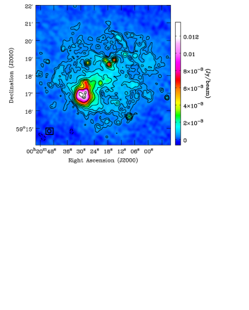
Figure 1: Total intensity map of IC 10 at 0.32 GHz observed using the GMRT with an angular resolution of $13\times 12$ arcsec². The beam is shown in bottom left hand corner. The contour levels are at $(-3,-2,3,4,6,10,16,24,32,50,80,85)\times 150~{}\mu$Jy beam^-1.

3 Observations and data analysis

3.1 GMRT data

We observed IC 10 using the Giant Metrewave Radio Telescope (GMRT) at 0.322 GHz ($\nu_{\rm RF}$ between 0.307 to 0.339 GHz) using the software backend having a bandwidth of 33.3 MHz split into 512 channels and a total on-source time of $\sim 7$ hours. The data was analyzed using the NRAO Astronomical Image Processing System (AIPS) following standard routines for data flagging and calibration. The phase solutions were iteratively obtained on a nearby bright phase calibrator, 3C 468.1. The solutions were transferred to the target source once the closure errors were less than 1 per cent. The phase calibrator 3C 468.1 has a flux density of 20.5 Jy at 0.32 GHz and was used to solve for the bandpass gains along with the flux calibrator 3C 147.

Several rounds of phase-only self-calibration were performed using the point sources in the target field. To achieve a reliable model of the point sources, we used only the baselines $\gtrsim 1$ k$\lambda$ and the data was weighted using Briggs’ robust parameter of $-1$ (Briggs, 1995). Final imaging was done using all baselines and employing the technique of polyhedron imaging for making wide-field images with non-coplanar baselines. To deconvolve the diffuse emission, we employed the sdi-clean algorithm (Steer et al., 1984) in AIPS and used a Briggs’ robust parameter of 0. In Fig. 1, we show the total intensity image of IC 10 at 0.32 GHz. The resolution of the image is $13\times 12$ arcsec² and has rms noise of $150~{}\mu$Jy beam^-1. The galaxy-integrated flux density is found to be 545$\pm$25 mJy and is in agreement with extrapolated flux densities from higher frequencies (see Fig. 2). Note that the largest angular scale detectable at 0.32 GHz by the GMRT is $\sim 18$ arcmin. Therefore, at the short baselines ($\rm\lesssim 0.2~{}k\lambda$), IC 10 is unresolved and hence we do not expect any missing flux-density of the diffuse emission in our observations and are only noise-limited.

Figure 2: Galaxy-integrated radio continuum spectrum of IC 10. The black data points are the flux densities measured at various frequencies (see Table 2). The black dashed line shows the classical power-law fit to the data having spectral index $-0.34\pm 0.01$. The green dotted line is the estimated thermal emission. The red points show the non-thermal flux densities after subtracting the thermal emission and the red line is the best-fit power-law with $\alpha_{\rm nt}=-0.55\pm 0.04$. The blue dot-dashed line is the best-fit to the non-thermal emission with a curved spectrum. The solid black and dot-dashed magenta curves are the total intensity spectrum estimated by adding the thermal emission to the non-thermal emission estimated by power-law and curved-spectrum, respectively.

3.2 Archival data at higher radio frequencies

3.2.1 1.42 GHz

We downloaded and analyzed archival dataset of IC 10 observed in 2004 with the NRAO Karl G. Jansky Very Large Array (VLA) in C-configuration using two side-bands of 50 MHz each, centered at 1.385 and 1.465 GHz (project code: AC717). The total on-source time was $\sim 5$ hours. Combining the two side-bands we obtain a map of IC 10 with 100 MHz bandwidth centered at 1.42 GHz. After standard data analysis we obtain a map rms noise of $\sim 35~{}\mu$Jy beam^-1 and an angular resolution of $17\times 16$ arscec².

From these observations, the total flux density of IC 10 at 1.42 GHz is found to be $270\pm 20$ mJy. At similar frequencies, the flux density measured by the NVSS data (Condon et al., 1998) is $300\pm 20$ mJy whereas Chyży et al. (2016) found a total flux density of $377\pm 11$ mJy, which includes a large extended synchrotron halo. We therefore believe that the archival C-configuration data suffers from missing flux density at $\gtrsim 20$ per cent level. However, the missing large angular scale emission does not affect the flux densities at small-scales, especially for sources that are unresolved. We therefore restricted the use of these data to study the spectrum of compact regions within the disc of IC 10.

3.2.2 6.2 GHz

IC 10 was observed using the VLA in D-configuration at a central frequency of 6.2 GHz (project code: AH1006; Heesen et al., 2015). To mitigate the effects of missing large-angular scale emission in these interferometric observations, single-dish data observed using the Effelsberg 100-m telescope were added to obtain total intensity image at $9.4\times 7.3$ arcsec² angular resolution and rms noise of $15~{}\mu$Jy beam^-1 (see Heesen et al., 2015, for details). The total flux density of the combined VLA+Effelsberg observations is found to be $186\pm 10$ mJy at 6.2 GHz.

3.3 Other ancillary data

3.3.1 H$\alpha$ map

We used H$\alpha$ emission of IC 10 to estimate the contribution of thermal free–free emission to the total radio continuum emission and to compute the star formation rate (SFR). A stellar-continuum subtracted H$\alpha$ image, observed using the Perkins 1.8-m telescope at the Lowell observatory (Hunter & Elmegreen, 2004), was downloaded from the NED. The image has an angular resolution of $2.2\times 2.2$ arcsec² and a brightness sensitivity of $10^{-18}~{}\rm erg\,s^{-1}\,cm^{-2}$ per 0.49 arcsec pixel-size. This corresponds to a star formation rate surface density of $1.1\times 10^{-4}~{}\rm M_{\odot}\,yr^{-1}\,kpc^{-2}$ (not corrected for extinction) at distance of 0.74 Mpc for IC 10.

3.3.2 Infrared maps

Spitzer MIPS 24 $\mu$m: To correct for internal dust extinction of the H$\alpha$ emission and to study the spatially resolved radio–IR relation, we used a $24\,\mu$m map observed using the Spitzer space telescope (Bendo et al., 2012). The map has an angular resolution of $6\times 6$ arcsec² and a $1\sigma$ flux density sensitivity of $0.25$ mJy beam^-1.
Herschel PACS 70 $\mu$m: To study the radio–IR relation using cold dust emission and estimate its temperature we used a far-infrared map of IC 10 at $70\,\mu$m. IC 10 was observed using the Herschel space telescope and we downloaded a level 2.5 data product from the NASA/IPAC Infrared Science Archive (IRSA). The $70\,\mu$m-map has an angular resolution of $5.2\times 5.2$ arcsec² with a $1\sigma$ flux density sensitivity of $\sim 6$ mJy beam^-1.
Herschel PACS 160 $\mu$m: For computing the dust temperature, in addition to the $70\,\mu$m map of IC 10, we downloaded a $160\,\mu$m-map observed using Herschel from the IRSA. The map was available with $12\times 12$ arcsec² angular resolution and a $1\sigma$ rms noise of $\sim 80$ mJy beam^-1.

3.4 Thermal emission separation

Since IC 10 has recently undergone an active burst of star formation (Vacca et al., 2007; Yin et al., 2010), the contribution of the thermal free–free emission to the total radio continuum emission could be significant. We estimated the thermal emission from IC 10 using the H$\alpha$ emission as its tracer, because it originates from the recombination of the same free electrons that produces the free–free emission. The thermal flux density ($S_{\rm th,\nu}$) at a radio frequency $\nu$ is related to the electron temperature ($T_{\rm e}$, assumed to be $10^{4}$ K) and the free–free optical depth ($\tau_{\rm ff}$) as,

$$S_{\rm th,\nu}=\frac{2\,k\,T_{\rm e}\nu^{2}}{c^{2}}(1-e^{-\tau_{\rm ff}}).$$ (1)

$\tau_{\rm ff}$ is related to the emission measure (EM) as,

$$\tau_{\rm ff}=0.082\,T_{\rm e}^{-1.35}\left(\frac{\nu}{\rm GHz}\right)^{-2.1}\left(\frac{\rm EM}{\rm cm^{-6}pc}\right),$$ (2)

where the EM is determined from the H$\alpha$ intensity ($I_{\rm H\alpha}$) following Valls-Gabaud (1998),

$$\left(\frac{I_{\rm H\alpha}}{\rm erg\,cm^{-2}s^{-1}sr^{-1}}\right)=9.41\times 10^{-8}T_{\rm e4}^{-1.017}10^{-0.029/T_{\rm e4}}\left(\frac{\rm EM}{\rm cm^{-6}pc}\right).$$ (3)

Here, $T_{\rm e4}$ is the electron temperature in units of $10^{4}$ K and, $k$ and $c$ are the standard constants.

Although the H$\alpha$ emission is the best tracer of the thermal emission, it is easily absorbed by the dust present both internal to the galaxy and in the Galactic foreground (Milky Way). The Galactic latitude of IC 10 is $-3.3^{\circ}$, and therefore Milky Way extinction is significant. The standard Schlegel et al. (1998) maps for estimating the Milky Way dust extinction are not useful below Galactic latitude $\sim 5^{\circ}$. Instead, we use the average value of $E(B-V)=0.77$ measured by Richer et al. (2001) in the direction of IC 10, which combined with an $R_{V}$ of $3.1$ gives the value for extinction at the wavelength of H$\alpha$ to be $A_{H\alpha}=1.95$. We apply this as the uniform Galactic extinction for IC 10. On the other hand, the internal extinction of the H$\alpha$ emission was accounted for by combining the extinction-corrected H$\alpha$ emission with 24-$\mu$m emission of IC 10 as (Kennicutt et al., 2009),

$$I_{\rm H\alpha,corr}=I_{\rm H\alpha,obs}10^{A_{\rm H\alpha}/2.5}+0.02\,\nu_{\rm 24\mu m}\,I_{\rm 24\mu m}.$$ (4)

Here, $I_{\rm H\alpha,obs}$ and $I_{\rm H\alpha,corr}$ are the observed and extinction-corrected H$\alpha$ intensities, respectively and $I_{\rm 24\mu m}$ is the intensity of the $24\,\mu$m emission. Due to the low metallicity of IC 10 ($Z\approx 0.2\,Z_{\odot}$, Garnett 1990), overall, the internal extinction is found to be $\lesssim 30$ per cent. Locally, the internal extinction can be up to 60 per cent in bright Hii regions while in the disc it lies in the range 5–20 per cent.

Both the H$\alpha$ and the $24\,\mu$m maps were convolved to a common angular resolution of 15 arcsec, determined by the radio continuum maps. They were then aligned to a common coordinate system. After correcting for dust extinction of the H$\alpha$ emission, the thermal emission was estimated on a pixel-by-pixel basis and subtracted from the total radio continuum emission at 0.32, 1.42 and 6.2 GHz. Overall, we estimate the thermal fraction, $f_{\rm th}$, to be $0.20\pm 0.05$, $0.35\pm 0.07$ and $0.53\pm 0.1$ at 0.32, 1.42 and 6.2 GHz, respectively. As mentioned in Section 3.2.1, the 1.42-GHz radio continuum map likely suffers from missing flux density and hence, $f_{\rm th,1.42\,GHz}$ is overestimated. However, this is not an issue at 0.32 and 6.2 GHz.

Uncertainty in the estimated thermal emission mainly arises from the extinction correction of the H$\alpha$ emission and from $T_{\rm e}$, which is not well known. Kennicutt et al. (2009) pointed out that the combination of H$\alpha$ and $24\,\mu$m emission suffers small systematic variation compared to reliable tracers of extinction such as the Balmer decrement and are within $\sim 15$ per cent on average. Moreover, because of the low metallicity of IC 10, the internal extinction is low and hence we do not expect significant uncertainty due to the internal attenuation correction. For example, assuming a 30 per cent uncertainty due to the internal extinction applied through Eq. 4, the maximum uncertainty to the thermal emission is $\sim 10$ per cent and is $\lesssim 5$ per cent over the H$\alpha$-emitting disc of IC 10.

On the other hand, the foreground Galactic reddening $E(B-V)$ in certain directions towards IC 10 can be as low as 0.37 or as high as 0.87 (see Richer et al., 2001). Thus, due to our assumed uniform value of $E(B-V)=0.77$ towards IC 10, there can a systematic error in the range $-60$ and $+25$ per cent to the thermal emission.

The unknown $T_{\rm e}$ can give rise to up to $\sim 10$ and $20$ per cent error in the estimated thermal emission at 0.32 and 6.2 GHz, respectively (see Tabatabaei et al., 2007b, for details). Overall, the estimated thermal emission and thereby $f_{\rm th}$ can have a systematic error up to $\sim 30$ per cent at 0.32 GHz and $\sim 50$ per cent at 6.2 GHz. However, errors in the thermal fraction affect the non-thermal emission less severely. For example, within the H$\alpha$-emitting disc of IC 10, an $f_{\rm th,6.2GHz}~{}(f_{\rm th,0.32GHz})$ of 0.5 (0.2) with an error of $30$ per cent gives rise to a 30 (10) per cent error on the non-thermal emission.

Clearly, a large error in a high $f_{\rm th}$ region will affect the non-thermal emission most. In Section 4.2.1 though, we show that the Hii regions showing 100 per cent thermal emission agree with our estimated thermal flux. Therefore, we believe that our estimated non-thermal emission maps do not suffer from large systematic errors.

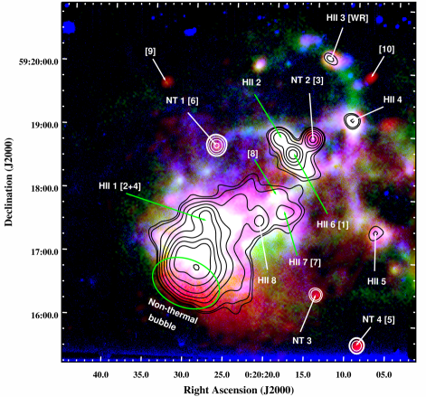
Figure 3: Various point sources detected at 0.32 GHz are marked on the composite image of IC 10 where the H$\alpha$, $70\,\mu$m and 6.2 GHz emissions are shown in blue, green and red colours, respectively. The contour levels show the total intensity at 0.32 GHz at $(8,9,13,19,27.5,38.5,52,68,86,107)\times 150~{}\mu$Jy beam^-1. The sources marked as Hii are the Hii regions, while the sources marked as NT are non-thermal emitting regions without any H$\alpha$ counterpart. The alternate nomenclature corresponding for some of these sources detected in the e-Merlin observations of Westcott et al. (2017) are given within the square brackets.

3.5 Star formation rate

To trace the recent star formation rate (SFR; $\lesssim 10$ Myr), we used the extinction corrected H$\alpha$ flux (in Eq. 4) to convert it into SFR by following the calibration given in Kennicutt & Evans (2012) based on Hao et al. (2011). It should be noted that the calibration is valid for star formation in solar metallicity environments. In order to account for the low metallicity of IC 10, we multiply the H$\alpha$ flux by a factor 0.89 before converting it into a SFR. This essentially accounts for the fact that, for a given SFR in a low metallicity environment, the escape fraction of H$\alpha$ photons is larger as compared to a higher metallicity environment. The factor 0.89 was deduced from Raiter et al. (2010) who estimated emergent fluxes in sub-solar metallicity environments for a Salpeter initial mass function (IMF; Salpeter, 1955; Chabrier, 2005) and constant star formation over at least the last $10^{8}$ years. The galaxy-integrated SFR was estimated to be $0.037\pm 0.003$ $\rm M_{\odot}\,yr^{-1}$. We however note, although the statistical error on our estimated SFR is low, the systematic error in the conversion factor of H$\alpha$ flux to SFR can vary by up to a factor of $\sim 2$ (Weilbacher & Fritze-v. Alvensleben, 2001; Hao et al., 2011).

4 Results

4.1 Total intensity

The total intensity radio continuum map of IC 10 at 0.32 GHz, shown in Fig. 1, is the highest angular resolution and sensitivity map available for IC 10 at frequencies below 1 GHz to date. Overall, the radio continuum emission of IC 10 at 0.32 GHz originates from a variety of structures and sources. In Fig. 3, we mark the point-like sources and the non-thermal bubble detected at 0.32 GHz on a composite colour image of IC 10 with H$\alpha$ emission from the Perkins 1.8-m telescope in blue, $70\,\mu$m emission from Herschel PACS in green and 6.2 GHz emission from VLA+Effelsberg in red. The Hii regions, mostly seen as white regions in the figure are marked as Hii 1–8. The brighter radio continuum emission regions in IC 10 are coincident with high SFR regions and giant molecular clouds (GMCs) detected in the survey of CO($J=1\to 0$) emission by Leroy et al. (2006). However, not all bright radio continuum emission originates from star forming regions, such as the non-thermal sources appearing reddish in Fig. 3 that are marked as NT 1–4. Several of these compact emitting regions are detected at 1.5 GHz in the high-resolution e-MERLIN observations by Westcott et al. (2017). The alternate nomenclature of the e-MERLIN detected sources are given within square brackets.

Table 2: Integrated flux density of IC 10.

Frequency	Flux density	References
(GHz)	(Jy)
0.32	$0.545\pm 0.025$	This paper (GMRT)
1.415	$0.304\pm 0.030$	1
1.42†	$>0.270$	This paper (VLA C-array)
1.43¶	$0.377\pm 0.011$	2
1.49	$0.30\pm 0.02$	NVSS
2.64	$0.250\pm 0.02$	3
4.85	$0.222^{+0.015}_{-0.025}$	7
6.2†	$0.131\pm 0.07$	6
6.2	$0.186\pm 0.010$	This paper (VLA+Effelsberg)
8.35	$0.183\pm 0.008$	2
10.45	$0.155\pm 0.016$	4
10.7	$0.165\pm 0.007$	5
24.5	$0.118\pm 0.018$	7

¹Shostak (1974), ²Chyży et al. (2016), ³Chyży et al. (2011), ⁴Chyży et al. (2003), ⁵Klein et al. (1983), ⁶Heesen et al. (2011), ⁷Klein & Gräve (1986).

^† These points are not included while fitting the spectrum as they suffer from missing flux density.

^¶ This point is not included while fitting the spectrum as this includes contribution from the halo unlike other data.

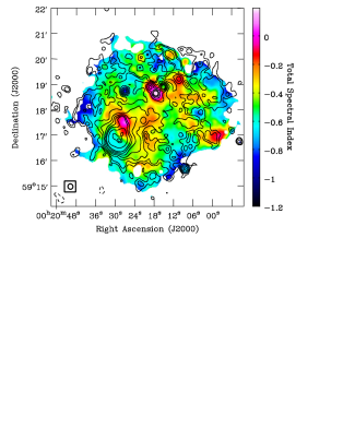
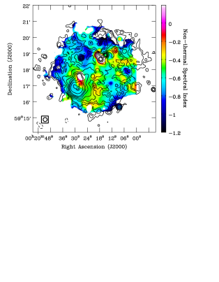
Figure 4: Left: Total spectral index map of IC 10 computed between 0.32 and 6.2 GHz using the total radio continuum emission. Both the maps were convolved to a common resolution of 15 arcsec and only the pixels $>3\sigma$ were considered. Right: Non-thermal spectral index map ($\alpha_{\rm nt}$) between 0.32 and 6.2 GHz at 15 arcsec angular resolution. The inner white regions are blanked where the total radio continuum emission is entirely thermal in nature. Pixels with $\alpha_{\rm nt}$ in the range $-0.4$ and $-0.1$ likely occur due to improper separation of the thermal emission. The contours are the total intensity contours at 0.32 GHz, same as Fig. 1.

Among the detailed studies at higher frequencies mentioned in Section 2, at 1.4 GHz Chyży et al. (2016) found evidence of a synchrotron halo extending up to $\sim 2.5$ kpc likely originating from magnetized winds driven by star formation. The rms noise of the map was 28 $\mu$Jy beam^-1 at an angular resolution of 26 arcsec. We made a lower resolution image of IC 10 at 0.32 GHz using baselines shorter than $\rm 10~{}k\lambda$ and convolved to 26 arcsec which rendered an image rms noise of $540~{}\mu$Jy beam^-1. At our sensitivity, the synchrotron halo remains undetected at 0.32 GHz. This implies that the spectral index of the halo around the $8\sigma$ contour of Chyży et al. (2016) map is $\gtrsim-1.0$ between 0.32 and 1.4 GHz for it to remain undetected at 0.32 GHz assuming a $2\sigma$ threshold. Thus, the CREs giving rise to the radio continuum emission are unlikely to be significantly affected by synchrotron and/or inverse-Compton losses. Chyży et al. (2016) suggested that a galactic wind with velocities $\sim 25~{}\rm km\,s^{-1}$ is responsible for the extended radio halo, i.e., the CREs would require $\sim 60$ Myr to travel to the edge of the halo at $\sim 1.5$ kpc (a wind velocity of $\sim 60~{}\rm km\,s^{-1}$ in turn would only need $\sim 25$ Myr to reach the same distance). Thus, the magnetic field strengths in the halo must be $\lesssim 5~{}\mu$G for the transport time-scales to be less than that of the synchrotron loss time-scale for the CREs emitting at 1.4 GHz to remain unaffected by synchrotron losses.

At 6.2 GHz, Heesen et al. (2011) found the radio continuum emission to closely trace the star forming regions. In particular, the Hii regions visible in the H$\alpha$ images are also bright at 6.2 GHz (marked as Hii $1-8$ in Fig. 3). They also found their radio continuum spectrum to be consistent with thermal emission, with $\alpha$ in the range $-0.1$ to $-0.2$. At 0.32 GHz, we detect these bright star-forming regions as well. Apart from these Hii regions, we also detect bright point-like sources in IC 10 that do not have any H$\alpha$ counterpart and are likely to be non-thermal sources (marked as NT $1-4$ in Fig. 3).

4.2 Thermal/non-thermal emission and spectral index

In Fig. 2, we plot the galaxy-integrated flux density of IC 10 between 0.32 and 24.5 GHz based on our measurements and data collected from the literature listed in Table 2. Overall, the radio continuum spectra of IC 10 is found to be flatter with spectral index $-0.34\pm 0.01$ than the $-0.7$ or steeper found in normal spirals. The green dotted line shows the estimated thermal emission as described in Section 3.4. The estimated $f_{\rm th}$ of $0.2\pm 0.05$ at 0.32 GHz is significantly higher than what is observed in normal star-forming galaxies at these frequencies (Basu et al., 2012a) and this high contribution of thermal free–free emission flattens the integrated spectra. The red points are the non-thermal flux density after subtracting the thermal emission at each frequency. The red dashed line is the best fit power-law to the non-thermal flux densities in the $\log$–$\log$ space and has a non-thermal spectral index ($\alpha_{\rm nt}$) of $-0.55\pm 0.04$. In order to assess any curvature in the non-thermal spectrum originating due to synchrotron and/or inverse-Compton losses, we also fitted a second-order polynomial of the form $\log S_{\rm\nu,nt}=s_{0}+\alpha_{\rm nt}\log\nu+\beta\,(\log\nu)^{2}$. The non-thermal radio continuum spectrum shows an indication of curvature and is shown as the blue dot-dashed curve in Fig. 2. We note that a curved spectrum fits the data marginally better than a single power-law. From the fit, the injection spectral index is found to be $-0.45\pm 0.05$ and is consistent with that of a fresh CRE population generated by diffusive shock acceleration (Bell, 1978; Blandford & Eichler, 1987).

In Fig. 4, left- and right-hand panels show the total and non-thermal spectral index maps of IC 10, respectively, estimated between 0.32 and 6.2 GHz. The bright point sources detected at 0.32 GHz, coincident with H$\alpha$ emission (marked as Hii $1-8$ in Fig. 3), have $\alpha$ values close to $-0.1$ or higher. This indicates that such sources are direct tracers of Hii regions and are dominated by thermal free–free emission. In fact, the sources marked as Hii 1, 2 and 6 exhibit broad-band spectra consistent with 100 per cent thermal emission. In Fig. 5, we show the map of the thermal fraction at 0.32 GHz ($f_{\rm th,0.32GHz}$) estimated by extrapolating the thermal emission with a constant thermal spectral index of $-0.1$. Clearly, $f_{\rm th,0.32GHz}$ in the location of Hii 1, 2, 4 and 6, i.e., the whitish regions in Fig. 5 are close to or exceed unity. We discuss the nature of the radio continuum spectra of these regions in detail in Section 4.2.1. As is also evident from the spectral index map, the regions with $\alpha\gtrsim-0.3$ in the disc of IC 10 closely follow the H$\alpha$ emission. The flat spectra are due to significant thermal emission where we find $f_{\rm th,0.32GHz}$ in the range 0.2 to 0.5 (see Fig. 5). The $\alpha_{\rm nt}$ in these regions are higher with values in the range $-0.5$ to $-0.6$, close to the injection spectral index of fresh CREs. The non-thermal radio emission from the H$\alpha$ emitting disc likely originates from young CREs produced during the star-burst.

The regions in the outer parts, i.e., outside the H$\alpha$ emitting disc, show a steeper radio continuum spectrum with $\alpha$ in the range $-0.4$ to $-0.8$. The thermal fractions are comparatively lower in the outer parts with $f_{\rm th}$ typically lying between 0.01 to 0.1 at 0.32 GHz and 0.1 to 0.2 at 6.2 GHz. The non-thermal spectrum in these regions is steep with $\alpha_{\rm nt}\lesssim-0.8$, indicating the CREs are likely affected by synchrotron losses.

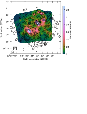
Figure 5: Thermal fraction map estimated at 0.32 GHz at 15 arcsec resolution. Overlaid contours are the total intensity 0.32 GHz emission same as Fig. 1.

Figure 6: Total intensity spectrum of some of the bright compact sources detected at 0.32 GHz marked in Fig. 3. The circles represents the sources Hii 1, 2 and 6 and are coincident with strong H$\alpha$ emission. The black triangles represents the observed total flux densities of the sources NT 1 and 2 which do not show enhanced H$\alpha$ emission. The grey triangles shows the non-thermal flux density after subtracting the thermal emission estimated at the positions of NT 1 and 2. All the errors are shown at $3\sigma$ level. The various dashed lines are the best representation of the spectrum for the corresponding sources. The dotted lines for the sources Hii 1, 2 and 6 are the extrapolated thermal flux density estimated using H$\alpha$ emission.

4.2.1 Free–free absorption

Some of the bright H$\alpha$ emitting regions show beam-averaged $f_{\rm th,0.32GHz}$ in the range 0.9 and 1.2, while at 6.2 GHz, no such region shows $f_{\rm th,6.2GHz}>1$. $\alpha$ in these regions have values $-0.1$ or higher. A close inspection of the total radio continuum emission at 0.32, 1.43 and 6.2 GHz reveals that the regions Hii 2 and 6 shows the effects of thermal free–free absorption which dominates at lower radio frequencies. In Fig. 6, we show the spectrum based on measurements at three frequencies of the brightest Hii regions, Hii 1, 2 and 6 and non-thermal sources NT 1 and 2. The sources Hii 2 and 6 clearly show lower radio continuum flux densities at 0.32 GHz compared to the extrapolated thermal emission estimated from the H$\alpha$ emission (shown as the dotted lines in Fig. 6), thereby giving rise to $f_{\rm th,0.32GHz}>1$ and $\alpha>-0.1$. For these two sources, the spectrum is best represented by an optically thick thermal free–free spectrum of the form $S_{\nu}=A\,\nu^{2}\,(1-e^{-m\,\nu^{-2.1}})$. While for the source Hii 1, the spectrum is consistent with an optically thin thermal free–free spectrum of the form $A\,\nu^{-0.1}$. The best-fit values of the parameters $A$ and $m$ are shown in Fig. 6.

For the sources Hii 2 and 6, comparing the best-fit parameter $m$ to Eqs. 1 and 2, we estimate the thermal free–free emission to be optically thick ($\tau_{\rm ff}\geq 1$) below $0.22\pm 0.03$ and $0.41\pm 0.05$ GHz, respectively. Recently, Hindson et al. (2016) in a study of Galactic Hii regions, found evidence of a turnover in the free–free spectrum typically with turnover frequencies in the range 0.3 to 1.2 GHz. We estimated the EM to be $(1.2\pm 0.3)\times 10^{5}$ and $(4.6\pm 1.2)\times 10^{5}~{}\rm pc\,cm^{-6}$ for Hii 2 and 6, respectively which in turn is related to the average thermal electron density $\langle n_{\rm e}\rangle$ as (Berkhuijsen et al., 2006):

$$\langle n_{\rm e}\rangle=\left(\frac{{\rm EM}\,{f}}{h_{\rm HII}}\right)^{1/2},$$ (5)

where, $f$ is the filling factor and $h_{\rm HII}$ is the size of the Hii region along the line of sight. Assuming a typical $f\sim 5$ per cent for the clumpy star-forming disc (Ehle & Beck, 1993) and $h_{\rm HII}\sim 50$ pc, i.e., the spatial resolution of our observations, we estimate $\langle n_{\rm e}\rangle$ to be $\sim 11$ and $22~{}\rm cm^{-3}$ for Hii 2 and 6, respectively, which are typical values for Hii regions (Hunt & Hirashita, 2009). Deeg et al. (1993) pointed out that such values of EM and $n_{\rm e}$ are necessary to explain the radio continuum spectra of star-forming blue compact dwarf galaxies. To better constrain $\langle n_{\rm e}\rangle$ and the sizes of the Hii regions, high resolution radio continuum observations at even lower frequencies with LOFAR will be necessary.

The thermal emission independently estimated using extinction corrected H$\alpha$ emission well represents the emission in the three Hii regions (shown as black dotted lines in Fig. 6). This suggests that the extinction corrected H$\alpha$ emission is a good tracer of the thermal free–free emission on scales below 100 pc. Since, the total radio continuum emission in these regions are already consistent with 100 per cent thermal emission, it is difficult to estimate the contribution of the non-thermal component. We have therefore blanked these pixels in our future calculations.

Figure 7: Total spectral index map between 0.32 and 6.2 GHz of the inner regions of IC 10. The locations of the GMCs found in the survey by Leroy et al. (2006) are shown as circles and crosses. The size of the circles are the same as the physical sizes estimated by Leroy et al. (2006), while for the crosses the size information was not available. The black line shows the sharp edge observed in the spectral index map coincident with the boundary of the molecular clouds. We also mark the compact sources marked in Fig. 3. The contours are the total intensity contours at 0.32 GHz drawn at $(15,25,40,50,60,70,80,85)\times 150~{}\mu$Jy beam^-1.

4.2.2 Non-thermal bubble

An interesting feature observed in the maps of $\alpha$ and $\alpha_{\rm nt}$ lies towards the south-eastern edge of IC 10 marked as the “non-thermal bubble” in Fig. 3. The bubble was first identified in the radio continuum observations of Yang & Skillman (1993). The sharp boundary of this region is distinctly visible only in the spectral index maps (see Fig. 4). The total intensity emission is merged with the bright Hii region Hii 1 and does not show the bubble distinctly. In Fig. 7 we show a zoomed-in view of the spectral index map. We mark the sharp boundary of the bubble and determine its center to be at RA=$00^{\rm h}20^{\rm m}29^{\rm s}$ and Dec.=$+59^{\circ}16^{\prime}39.5^{\prime\prime}$. The non-thermal bubble extends $\sim 300$ pc in the north-east to south-west direction and $\sim 100$ pc in the north-west to south-east direction. Its north-western edge, where the spectrum flattens from being non-thermal with $\alpha\sim-0.6$ to thermal $\alpha\sim-0.1$, is bound by giant molecular clouds (GMCs) as observed by Leroy et al. (2006), shown as the black circles in Fig. 7. This suggests that the GMCs likely confine the CREs in the bubble. This sharp feature is also visible in the spectral index map computed between 1.43 and 4.86 GHz using a completely independent dataset (Chyży et al., 2016).

The strongest non-thermal emission in IC 10 originates from the bubble both at 0.32 and 6.2 GHz. $f_{\rm th}$ in this region is lower than the other parts in the disc of IC 10 with $f_{\rm th}\sim 0.035$ and $0.16$ at 0.32 and 6.2 GHz, respectively. Apart from the outer edges of IC 10 where $f_{\rm th}$ tends to be on the low side, this is the only region within the H$\alpha$ emitting disc which is dominated by non-thermal emission. The average $\alpha$ and $\alpha_{\rm nt}$ between 0.3 and 6.2 GHz in the bubble is found to be $-0.61\pm 0.02$ and $-0.66\pm 0.03$, respectively. Compared to the diffuse emission in the outer parts of IC 10, the non-thermal spectrum is slightly flatter in the bubble. Using broadband data, Heesen et al. (2015) modelled the radio continuum spectrum of the bubble using a Jaffe–Perola model (Jaffe & Perola, 1973). Their modelling yielded an injection spectral index of $-0.6\pm 0.1$, consistent with the non-thermal spectral index measured in our observations. This indicates that the CREs giving rise to the synchrotron emission in the bubble are freshly generated.

4.2.3 Non-thermal point-like sources

Apart from the bright Hii regions, we also find a few bright knots at 0.32 GHz which do not show strong H$\alpha$ emission. Unlike the diffuse non-thermal bubble, these sources are compact and appear to be point-like (marked as NT 1, 2, 3 and 4 in Fig. 3). These regions show locally enhanced non-thermal emission and the thermal fractions are low with $f_{\rm th,0.32GHz}$ in the range 0.05–0.08 (see Fig. 5). The spectral index of their total radio continuum emission lies in the range $-0.8$ to $-0.5$, which is smaller than the main H$\alpha$ emitting disc of IC 10. The total intensity spectra for two of the sources NT 1 and 2 are shown in Fig. 6 which are distinctly different from a thermal spectrum. Because of their steep spectra, these point-like sources are not prominently visible in the images at 1.42 and 6.2 GHz (Chyży et al., 2016; Heesen et al., 2011). Non-thermal sources NT 1, 2 and 4 are detected by e-MERLIN observations and are shown to be compact sources. They are likely to be background star-forming galaxies, hosting active galactic nuclei (Westcott et al., 2017).

4.3 Magnetic field strengths

We computed the total magnetic field strength ($B_{\rm tot}$) of IC 10 on a pixel-by-pixel basis using the non-thermal emission and $\alpha_{\rm nt}$ maps assuming energy equipartition between cosmic ray particles and the magnetic field (Beck & Krause, 2005). We assumed the ratio of number densities of relativistic protons to electrons ($K$) to be 100 and the path-length of the synchrotron emitting media ($l$) to be 1 kpc and corrected this for the galaxy’s inclination. In Fig. 8 we present the total magnetic field strength map of IC 10. The average field strength within the $3\sigma$ region (excluding the background non-thermal sources, NT 1, 2 and 4 and the Hii regions with 100 per cent thermal emission) is estimated to be $\sim 10~{}\mu$G. Our estimated field strengths are lower than the average field strength of $14~{}\mu$G estimated by Chyży et al. (2016). Note that, Chyży et al. (2016) found the field to be strongest ($\sim 29~{}\mu$G) in the Hii complex (marked as Hii 1 in Fig. 3). However, our study shows that this region has 100 per cent thermal emission and the assumption of energy equipartition is invalid and hence has been blanked in Fig. 8.

We find the magnetic fields to be the strongest in the non-thermal bubble with field strengths of $\sim 20~{}\mu$G, similar to Chyży et al. (2016). However, the field strengths could be higher in this region as the bubble is unlikely to extend 1 kpc along the line of sight (see Heesen et al., 2015).

In the H$\alpha$-emitting disc, the field strength lies in the range 10 to $15~{}\mu$G and falls off to $\sim 8~{}\mu$G in the outer parts. Excluding the non-thermal bubble, the average field is estimated to be $\sim 12~{}\mu$G in the mid-plane. The estimated magnetic field strengths in IC 10 are larger than those typically observed in dwarf irregular galaxies ($\lesssim 5~{}\mu$G; Chyży et al. 2011) and comparable to those observed in normal spiral galaxies ($9-15~{}\mu$G; Basu & Roy 2013).

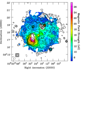
Figure 8: Total magnetic field strength of IC 10 estimated assuming energy equipartition between cosmic ray particles and magnetic field. The inner white regions are blanked because of uncertainty in the estimation of non-thermal emission. The overlaid contours are the total intensity emission at 0.32 GHz (same as Fig. 1; see text for details).

Note that, our estimated magnetic field strengths can be scaled by a factor $[10^{-2}(K+1)\times\Delta f_{\rm nth}/l]^{1/(3-\alpha_{\rm nt})}$ because of our assumed values of $K$ and $l$. Thus, a factor of 2 difference in the path length would give rise to a maximum of $\sim 22$ per cent systematic error in the magnetic field strength. On the other hand, the statistical error of the magnetic field strength depends on the signal-to-noise ratio (SNR) of the non-thermal emission. Typically, in the high SNR regions ($\gtrsim 5$), i.e., within the H$\alpha$-emitting disc of IC 10, the error lies in the range $2-10$ per cent, while in the outer parts with SNR 3–5, the error can be up to $\sim 20$ per cent. Further, to include an error in the estimated thermal emission, we consider the term $\Delta f_{\rm nth}$ defined as $\Delta f_{\rm nth}=1\pm df_{\rm nth}/f_{\rm nth}$, where $df_{\rm nth}$ is the error on the estimated non-thermal fraction ($f_{\rm nth}=1-f_{\rm th}$). In terms of $f_{\rm th}$, $\Delta f_{\rm nth}$ is given as $\Delta f_{\rm nth}=[1-(1\pm a)f_{\rm th}]/[1-f_{\rm th}]$, where $a$ is the relative error on $f_{\rm th}$. An error of 30 per cent on $f_{\rm th}$ (i.e., $a=\pm 0.3$) in a region with $f_{\rm th}=0.5(0.2)$ gives rise to less than $10(3)$ per cent error on the magnetic field strength. Overall, the error on the estimated magnetic field strength is $\lesssim 10$ per cent within the H$\alpha$-emitting disc of IC 10 and up to $\sim 20$ per cent in the outer parts.

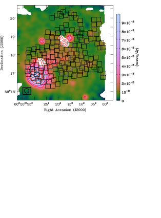
Figure 9: Non-thermal emission map at 0.32 GHz at 15 arcsec resolution. The inner white pixels are blanked as they correspond to the location of Hii regions with 100 per cent thermal emission (see Section 4.2.1). The boxes represent regions within which the our spatially resolved studies are performed and are roughly of one beam-size. Overlaid red contours are the total intensity 0.32 GHz emission same as Fig. 7.

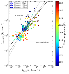
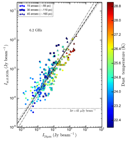
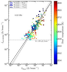
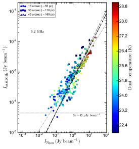
Figure 10: Spatially resolved non-thermal radio continuum intensity vs. MIR intensity at $24\,\mu$m (top panels) and, vs. FIR intensity at $70\,\mu$m (bottom panels). The left-hand and right-hand sides are for the emission at 0.32 and 6.2 GHz, respectively. The circle, square and triangle symbols are averaged over 15, 30 and 45 arcsec apertures, respectively. The dash-dotted lines are the best fit lines in the $\log-\log$ space, where the light grey, grey and black lines are for 15, 30 and 45 arcsec, respectively. The $3\sigma$ detection threshold for the non-thermal emission is shown as a dotted line. The points are coloured based on the dust temperature.

Table 3: Summary of spatially resolved radio–infrared relation in IC 10. The slopes ($b$) and $\log a$ are obtained by fitting the non-thermal radio continuum versus IR intensities as $I_{\rm nt,\nu}=a\times I_{\rm IR}^{b}$ in the $\log$–$\log$ space. $\sigma_{\rm IR}$ is the dispersion around the fit after normalizing $x-$ and $y-$axis to their median values and is a measure of the scatter or “tightness” of the corresponding relation.

	Spatial scale
	55 pc					110 pc					165 pc
Frequency	$r_{S}$	Slope	$-\log\,a$	$\sigma_{\rm IR}$		$r_{S}$	Slope	$-\log\,a$	$\sigma_{\rm IR}$		$r_{S}$	Slope	$-\log\,a$	$\sigma_{\rm IR}$
	Using 24 $\mu$m MIR emission
0.32 GHz	0.47	$0.97\pm 0.15$	$1.15\pm 0.28$	4.36		0.52	$0.77\pm 0.13$	$1.52\pm 0.16$	2.51		0.68	$0.65\pm 0.10$	$1.58\pm 0.09$	1.34
6.2 GHz	0.73	$0.80\pm 0.06$	$2.16\pm 0.11$	2.63		0.73	$0.91\pm 0.09$	$2.08\pm 0.11$	2.38		0.82	$0.83\pm 0.10$	$2.14\pm 0.07$	1.34
	Using 70 $\mu$m FIR emission
0.32 GHz	0.62	$0.93\pm 0.09$	$2.43\pm 0.06$	2.42		0.68	$0.88\pm 0.11$	$2.46\pm 0.02$	1.79		0.79	$0.82\pm 0.11$	$2.42\pm 0.05$	1.08
6.2 GHz	0.84	$0.87\pm 0.04$	$3.14\pm 0.03$	1.66		0.83	$1.12\pm 0.09$	$3.19\pm 0.03$	1.52		0.89	$1.08\pm 0.11$	$3.23\pm 0.07$	0.93

4.4 Spatially resolved radio–infrared relations

We studied the well known radio–infrared relations in IC 10 at angular resolutions of 15, 30 and 45 arcsec, corresponding to spatial scales of $\sim 55$, 110 and 165 pc, respectively. We used the non-thermal emission maps at 0.32 and 6.2 GHz and mid- and far-infrared (MIR and FIR) maps at 24 and $70\,\mu$m, respectively. The radio–FIR and radio–MIR relations are thought to be of different physical origin. The radio–FIR relation arises primarily due to the coupling between magnetic field and gas density (Niklas & Beck, 1997; Schleicher & Beck, 2013, 2016), while the radio–MIR relation is a consequence of star formation (Heesen et al., 2014). We therefore expect different dispersions for the two types of relations.

The infrared maps were convolved to the resolution of the non-thermal radio maps, i.e., 15 arcsec, using the convolution kernels given by Aniano et al. (2011). Both the non-thermal radio and IR intensities were computed averaged over regions of one beam size. To ensure independence, the regions were separated roughly by one beam and only the pixels above $3\sigma$ rms noise of the non-thermal radio maps were considered. The regions within which the averaging was done are shown in Fig. 9 and are overlaid on the non-thermal emission map at 0.32 GHz at 15 arcsec resolution. To ensure that our results are least affected due to insufficient thermal emission separation, all the beams with $\alpha_{\rm nt}\geq-0.45$ were excluded from our further analysis. Further, we avoided all such beams which contained the non-thermal point-like sources and Hii regions with 100 per cent thermal emission. A similar approach was followed for analysis at 30 and 45 arcsec angular resolutions.

In Fig. 10 we plot the non-thermal radio intensities versus the IR intensities. The left- and right-hand panels are for 0.32 and 6.2 GHz, respectively, while the top and bottom panels are versus 24 and $70\,\mu$m, respectively. The circle, square and triangle symbols are averaged over 15, 30 and 45 arcsec, respectively and they are coloured based on the dust temperature ($T_{\rm dust}$; see Section 5.2). The error on the data points are smaller than the scatter of the plots. The non-thermal emission at 6.2 GHz and the MIR emission at $24\,\mu$m of IC 10 is found to be strongly correlated with Spearman’s rank correlation, $r_{\rm S}=0.73$ at $\sim 55$ pc spatial scale and increases slightly with $r_{\rm S}=0.82$ at $\sim 110$ and 165 pc scales. At 0.32 GHz, the correlation is weaker with $r_{\rm S}=0.47,0.52$ and $0.68$ at $\sim 55,110$ and 165 pc spatial scales, respectively. However, we note that the 0.32-GHz non-thermal emission is limited by noise. Deeper observations are required to study the true span and nature of the correlation at lower frequencies. At 6.2 GHz, the noise is not a limitation and the correlation can be studied in greater detail.

On the other hand, the non-thermal radio emission at both frequencies correlates significantly better with FIR emission at $70\,\mu$m as compared to the MIR emission. The $r_{\rm S}$ between $I_{\rm 70\mu m}$ and $I_{\rm 6.2GHz}$ lies in the range 0.83 and 0.89 for the three spatial scales probed in our study. At 0.32 GHz, the correlation with the $70\,\mu$m emission is significantly stronger than with $24\,\mu$m, and $r_{\rm S}$ increases from 0.62 at 55 pc scale to 0.79 at 165 pc scale.

We fitted the data with the form $I_{\rm nt,\nu}=a\,I_{\rm IR}^{b}$ in $\log-\log$ space ($\log\,I_{\rm nt,\nu}=b\times\log\,I_{\rm IR}+\log\,a$) using the ordinary least-square bisector method (Isobe et al., 1990). Separate fits were performed for each of the spatial scales, and the best fits are shown as dash-dotted lines in Fig. 10. In Table 3, we summarize the results of the radio–infrared relations. The parameter $\sigma_{\rm IR}$ in Table 3 is a measure of the scatter or conversely the “tightness” of the relations and is defined as the dispersion around the fit to the data. Since, the absolute value of the dispersion would depend on the choice of units of the non-thermal radio and infrared intensities, we have normalized each axis by its median value before computing $\sigma_{\rm IR}$. One common feature is that the relation on all spatial scales probed in our study shows stronger correlation at 6.2 GHz with up to a factor of 1.6 lower dispersion around the median compared to that at 0.32 GHz. The dispersion decreases systematically at both the radio frequencies with increasing spatial scales which is due to the fact that small-scale fluctuations are smoothed out on large-scales.

Furthermore, we find that the dispersion around the median of the radio–FIR relation is lower by more than $\sim 30$ per cent as compared to that of the radio–MIR relation. This indicates that the colder dust emitting at $70\,\mu$m correlates better with non-thermal radio emission as compared to warmer dust emitting at $24\,\mu$m. Nevertheless, our result is consistent with Heesen et al. (2014), who pointed out that the $24\,\mu$m emission arises from dust heated by star formation activity. Hence, a hybrid indicator of star formation, i.e., $24\,\mu$m with far-ultraviolet or H$\alpha$ correlates better with the radio continuum emission as compared to monochromatic emission at $24\,\mu$m.

The slope of the relation between 0.32 GHz and infrared emission at both IR wavelengths are observed to decrease from roughly linear to sub-linear with increasing spatial scales. However, within the errors and the noise limitation of the 0.32 GHz non-thermal emission, this trend is inconclusive. On the other hand, at 6.2 GHz, within the errors, the slope of the relation with $24$ emission, remains roughly similar with a value of $\sim 0.85$ for all three spatial scales. The slope with the $70\,\mu$m emission is found to be slightly steeper. The slope of the correlation between FIR and non-thermal emission at both the radio frequencies are similar within $1.7\sigma$, on all three scales.

5 Discussion

5.1 The galaxy-integrated spectrum

The total intensity radio continuum spectrum of IC 10 between 0.32 and 24.5 GHz is consistent with a power-law with $\alpha=-0.34\pm 0.01$. The rather flat shape of this integrated spectrum is due to a high contribution from thermal free–free emission. After subtracting the thermal emission, the non-thermal spectrum is found to be consistent with a power-law with $\alpha_{\rm nt}=-0.55\pm 0.04$. A slight indication of the non-thermal spectrum being curved is also present. The overall difference between $\alpha$ and $\alpha_{\rm nt}$ is consistent with what was observed in spatially resolved galaxies at $\sim 1$ kpc scales in high thermal fraction regions (Basu et al., 2012a).

A cursory look at Fig. 4 immediately shows the limited usefulness of galaxy-integrated spectra or spectra that are spatially resolved but averaged over $\sim 0.5-1$ kpc, a typical linear scale probed by the currently available telescopes in nearby star-forming galaxies. Our study of IC 10 on $\sim 50$ pc spatial scale, comparable to the sizes of GMCs and star-burst regions, shows the importance of aiming for a spatial resolution that is matched to the relevant physical processes.

Observations at a spatial resolution of 50 pc such as presented here on IC 10 show that the galaxy-integrated spectrum is due to a combination of emission from a non-thermal bubble, optically thick and thin free–free emission from Hii regions, non-thermal emission from recently injected CRE and diffuse emission from older CRE as one moves away from the disc. It is therefore difficult to relate the spectral index values measured on kilo-parsec scales or larger with one particular physical process, as pointed out by Basu et al. (2015a) for normal star-forming galaxies. Nearby dwarf irregular galaxies offer an opportunity to make a comparative study of various emission mechanisms.

5.2 “Tightness” of the radio–FIR relation: a conspiracy

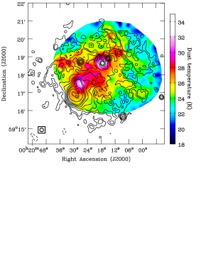
Figure 11: Distribution of $T_{\rm dust}$ in IC 10 obtained by fitting a modified Planck spectrum between 70 and $160\,\mu$m.

An interesting feature of our study is that, the relation between non-thermal emission at both 0.32 and 6.2 GHz with that of the FIR emission shows similar slopes (within $1.7\sigma$) and dispersions (differing by $\lesssim 50$ per cent) on all the three spatial scales probed in our study. This is surprising because propagation of CREs and scattering of ultraviolet (UV) photons would result in mixing of different populations originating from different star formation regions in IC 10. Effects of CRE propagation is expected to be larger for lower energy CREs emitting at 0.32 GHz, which could lead to the slope of the radio–FIR relation being flatter when studied at 0.32 GHz as compared to that at a higher frequency such as 6.2 GHz (see Basu et al., 2012b; Tabatabaei et al., 2013).

The ratio of the flux density at FIR wavelength ($\lambda_{\rm FIR}$) to that of the non-thermal emission at a radio frequency $\nu$, $I_{\lambda_{\rm FIR}}/I_{\rm nt,\nu}$, known as the ‘$q$’ parameter, is often used to study the dispersion of the radio–FIR relation (see e.g., Yun et al., 2001; Appleton et al., 2004; Ivison et al., 2010a, b; Basu et al., 2015b), although, for a non-linear slope of the radio–FIR relation, $q$ depends on the radio flux densities and is not suitable for quantifying the correlation (Basu et al., 2015b). However, it can be easily shown that $q$ is related to $B_{\rm tot}$, $\alpha_{\rm nt}$ and the dust temperature ($T_{\rm dust}$) as,

$$q\equiv\frac{I_{\lambda_{\rm FIR}}}{I_{\rm nt,\nu}}\propto\left(\frac{n_{\rm UV}}{n_{\rm CRE}}\right)\,\left(\frac{B_{\lambda_{\rm FIR}}(T_{\rm dust})\,Q(\lambda,a)}{B_{\rm tot}^{(1-\alpha_{\rm nt})}}\right),$$ (6)

provided both the FIR and radio emission originate from the same volume. Here, $n_{\rm UV}$ and $n_{\rm CRE}$ are the number densities of UV photons and CREs, respectively. $B_{\lambda_{\rm FIR}}(T_{\rm dust})$ is the Planck function and $Q(\lambda_{\rm FIR},a)$ is the wavelength dependent absorption coefficient for dust grains of radius $a$. Assuming similar dust grain properties and optically thin dust emission throughout IC 10, $Q\propto\lambda_{\rm FIR}^{-\beta}$, where we adopt a typical value for the dust emissivity index $\beta=2$ (Draine & Lee, 1984).

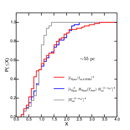
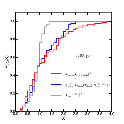
Figure 12: Cumulative distribution function of $X=I_{\rm 70\mu m}/I_{\rm nt,\nu}$ (shown in red), $X=\lambda_{\rm 70\mu m}^{-\beta}\,B_{\rm\lambda_{\rm 70\mu m}}(T_{\rm dust})\,B_{\rm tot}^{-(1-\alpha_{\rm nt})}$ (shown in blue) and $X=B_{\rm eq}^{-(1-\alpha_{\rm nt})}$ (shown in grey) for $\nu=6.2$ GHz (top panels) and $\nu=0.32$ GHz (bottom panels). The left-hand plots are computed for an aperture of 15 arcsec, i.e., averaged over spatial scale of $\sim 55$ pc, while the right-hand plots are averaged over 45 arcsec apertures corresponding to $\sim 165$ pc. The $[...]^{\star}$ indicates the quantities are normalized to their median values, i.e., $[X]^{\star}=X/{\rm median}(X)$.

Following Tabatabaei et al. (2007b), we determine an indicative $T_{\rm dust}$ by fitting a modified Planck spectrum to the cold dust emission between 70 and $160\,\mu$m on a pixel-by-pixel basis using Herschel PACS FIR maps. In Fig. 11, we present the $T_{\rm dust}$ map of IC 10 at a resolution of 15 arcsec. We find the mean value of $T_{\rm dust}$ to be $\sim 25$ K and it varies widely within IC 10 having values $\sim 20$ K in the outer parts and reaching up to $\sim 35$ K in the Hii regions. $T_{\rm dust}$ in IC 10 and its variation is larger than what is observed in normal star-forming galaxies ($T_{\rm dust}$ in the range 18–25 K; Tabatabaei et al. 2007a; Basu et al. 2012a; Kirkpatrick et al. 2014) and is consistent with what is observed in low-metallicity dwarf galaxies ($T_{\rm dust}$ in the range 21–98 K; Rémy-Ruyer et al. 2013; Madden et al. 2016).

To understand the origin of the scatter of the radio–FIR correlation, in Fig. 12 we plot the median normalized cumulative distribution function of $I_{\rm 70\mu m}/I_{\rm nt,\nu}$ (red lines) and compare it to the median normalized quantities $\lambda_{\rm 70\mu m}^{-\beta}\,B_{\rm 70\mu m}(T_{\rm dust})\,B_{\rm tot}^{-(1-\alpha_{\rm nt})}$ (blue lines) and $B_{\rm tot}^{-(1-\alpha_{\rm nt})}$ (grey lines). The top and bottom panels are for non-thermal emission at 6.2 and 0.32 GHz, while the left and right sides are averaged over 55 and 165 pc spatial scales, respectively. In the figure, we indicate the corresponding median normalized quantities as $[I_{\rm 70\mu m}/I_{\rm nt,\nu}]^{\star}$, $[\lambda_{\rm 70\mu m}^{-\beta}\,B_{\rm 70\mu m}(T_{\rm dust})\,B_{\rm tot}^{-(1-\alpha_{\rm nt})}]^{\star}$ and $[B_{\rm tot}^{-(1-\alpha_{\rm nt})}]^{\star}$. Clearly, the fluctuations of $B_{\rm tot}$ alone are insufficient to produce the dispersion observed for the correlation between the non-thermal radio emission and cold dust emission at $70\,\mu$m. However, on all the scales probed in our study, the combined fluctuations of $T_{\rm dust}$ and $B_{\rm tot}$ can well reproduce the distribution of $[I_{\rm 70\mu m}/I_{\rm nt,\nu}]^{\star}$.

On 165 pc scale, the fluctuations of $B_{\rm tot}$ reproduce the dispersion around the median $[I_{\rm 70\mu m}/I_{\rm nt,\nu}]^{\star}$ better, compared to its fluctuations on smaller scales, as the variations of $T_{\rm dust}$ are then lower. This is similar to what is observed on kiloparsec scales in normal star-forming galaxies. At such scales, the variations of $T_{\rm dust}$ are small and variations in $B_{\rm tot}$ alone are sufficient to reproduce the dispersion in the radio–FIR relation (Basu & Roy, 2013). Hence, our results reveal an important fact that the tightness of the radio–FIR arises due to a conspiracy between magnetic field and dust temperature variations on small scales, while on larger scales, magnetic fields and its coupling with ISM parameters is responsible. This is evident from Fig. 13 where we find the magnetic field strength and dust temperature to show mild correlation on smaller scales, while on larger scales the correlation is weaker. This is manifestation of the fact that dust temperature increases with star formation rate (Magnelli et al., 2014) and the local magnetic field is related to the local star formation rate (see Section 5.4).

Since, the CREs emitting at 0.32 GHz typically have propagation scale-length $\sim 2-4$ times larger than those emitting at 6.2 GHz, depending on whether they are transported by diffusion or advection at Alfvén speed, one would expect the dispersion of the radio–FIR relation to be significantly larger at 0.32 GHz. However, in contrary, we find that the distribution of the radio–FIR relations at both the radio frequencies are already well reproduced by invoking the variations of both $B_{\rm tot}$ and $T_{\rm dust}$, on scales $\gtrsim 55$ pc. This suggests, as per Eq. 6, that the fluctuations of $n_{\rm UV}/n_{\rm CRE}$ are small and thus, both CRE transport length ($l_{\rm CRE}$) and the mean-free path of UV photons ($l_{\rm mfp}$) are smaller than $\sim 55$ pc.

In a typical ISM, $l_{\rm mfp}$ is $\sim 20-100$ pc, roughly the size of the Strömgren sphere ionized by OB stars (Osterbrock & Ferland, 2006). Hence, scattering of UV photons are unlikely to be significant. On the other hand, since the magnetic fields in the disc of IC 10 are predominantly tangled (Chyży et al., 2016), the CREs are expected to be transported via the streaming instability at the Alfvén speed, $V_{\rm A}=B_{\rm tot}/\sqrt{4\,\pi\,\rho_{\rm gas}}\sim 12~{}\rm km\,s^{-1}$. The gas density $\rho_{\rm gas}\sim 8.6\times 10^{-24}~{}\rm g\,cm^{-3}$ was estimated from a Hi surface density map of IC 10. Therefore, for $l_{\rm CRE}$ to be smaller than $\sim 55$ pc, the CREs must have been produced $\lesssim 5$ Myr ago, consistent with the starburst scenario proposed by Vacca et al. (2007) and also with the spectral ageing analysis by Heesen et al. (2015). The young population of CREs in IC 10 gives rise to $\alpha_{\rm nt}\sim-0.5$ observed within the disc.

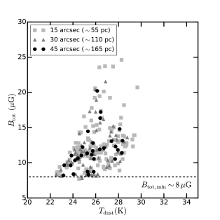
Figure 13: Total magnetic field ($B_{\rm tot}$) as a function of dust temperature ($T_{\rm dust}$) in IC 10. Squares, triangles and circles represents averaging over 55, 110 and 165 pc spatial scales. The dashed line represents the lower limit on magnetic field strength detectable by our observations at $3\sigma$ level.

5.3 Slope of the radio–FIR relation and $B_{\rm tot}$–$\rho_{\rm gas}$ relation

Under the condition of energy equipartition between magnetic field and kinetic energy of the turbulent gas, MHD simulations reveal that the magnetic field ($B_{\rm tot}$) and gas density ($\rho_{\rm gas}$) are coupled as $B_{\rm tot}\propto\rho_{\rm gas}^{\kappa}$, where $\kappa\sim 0.4-0.7$ (Chandrasekhar & Fermi, 1953; Mouschovias, 1976; Fiedler & Mouschovias, 1993; Cho & Vishniac, 2000; Kim et al., 2001). Building on the theory first proposed by Niklas & Beck (1997), Dumas et al. (2011) showed that, in the optically thin regime, the slope of the radio–FIR relation, $b$, the Kennicutt-Schmidt (KS) power law index, $n$, connecting the star formation rate and gas surface densities, and $\alpha_{\rm nt}$ are related to $\kappa$ as:

$$\kappa=\frac{(n+1)\,b}{(3-\alpha_{\rm nt})}.$$ (7)

This relation is valid provided both radio and FIR emission originate from the same emitting volume. In the previous section we argued, in IC 10 the non-thermal radio emission at 6.2 GHz and the FIR emission at $70\,\mu$m are correlated due to coupling of magnetic fields with the ISM on $\sim 165$ pc scale. Therefore, we use the slope of the radio–FIR relation $b=1.08\pm 0.11$, on 165 pc scale and, the mean value and dispersion of the observed $\alpha_{\rm nt}=-0.62\pm 0.15$. In dwarf irregular galaxies such as IC 10, the gas density is dominated by atomic Hi and the galaxy-averaged KS relation’s index $n$ is found to be $0.91^{+0.23}_{-0.25}$ (Roychowdhury et al., 2014). However, to compare with our spatially resolved study, we determine the index of the spatially resolved KS relation for IC 10 as $1.15\pm 0.06$. Using these values we estimate $\kappa=0.64\pm 0.17$ which is consistent with numerical simulations of a turbulent ISM. This indicates that the assumption of energy equipartition between magnetic field and cosmic ray particles is valid on 165 pc scales. Such a relation was confirmed in normal star-forming spiral galaxies at a spatial scale of $\sim 1$ kpc, i.e., the diffusion scale-length of CREs emitting at 1.4 GHz (Basu et al., 2012b). For the first time we confirm this relation in a dwarf irregular galaxy on sub-kpc scales.

5.4 Magnetic field and star formation: $B_{\rm tot}$–$\Sigma_{\rm SFR}$ relation

Recently, in a semi-analytical model to explain the correlation between radio and FIR emission, Schleicher & Beck (2013, 2016) pointed out that the correlation is mainly driven by the coupling between magnetic fields and surface density of star formation rate ($\Sigma_{\rm SFR}$) of the form $B_{\rm tot}\propto\Sigma_{\rm SFR}^{1/3}$. The coupling is established due to star-formation driven turbulent amplification of the magnetic field through the fluctuation dynamo operating on small-scales ($\lesssim 1$ kpc). In Fig. 14, we plot the spatially resolved total magnetic field strength as a function of the $\Sigma_{\rm SFR}$ in IC 10. We used the H$\alpha$ map, as explained in Section 3.5, to create a map of $\Sigma_{\rm SFR}$. We find the magnetic field strength to be strongly correlated with $\Sigma_{\rm SFR}$ having $r_{S}=0.7$ on 55 pc scales. Using the bisector method fit in $\log$–$\log$ space we find,

$$\left(\frac{B_{\rm tot}}{\rm\mu G}\right)=(51\pm 6)\left(\frac{\Sigma_{\rm SFR}}{\rm M_{\odot}\,yr^{-1}\,kpc^{-2}}\right)^{0.35\pm 0.03}.$$ (8)

The power-law index is similar to what is expected for star-brust driven turbulent amplification of the magnetic field $B_{\rm tot}$ and is likely responsible for establishing the radio–FIR correlation on sub-kpc scales (Schleicher & Beck, 2013, 2016).

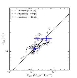
Figure 14: Total magnetic field ($B_{\rm tot}$) as a function of surface star formation rate ($\Sigma_{\rm SFR}$) in IC 10. The statistical error on the data points are smaller than the scatter of the plot. However, a systematic error up to factor of 2 for SFR calibration can be present. The blue stars are $\Sigma_{\rm SFR}$ determined on 165 pc scales and are binned in $B_{\rm tot}$ such that the total $\rm SFR$ in each bin is $\geq\rm 10^{-2.5}\,M_{\odot}\,yr^{-1}$. The dashed line is the bisector fit to the data points averaged over 15 arcsec in $\log-\log$ space. The best-fit power-law is found to be $(51\pm 6)\,{\Sigma_{\rm SFR}^{0.35\pm 0.03}}$.

By comparing simulation results of synthesized stellar populations (da Silva et al., 2012) with that of SFR indicators, da Silva et al. (2014) found that, for $\rm SFR\lesssim 10^{-2.5}\,M_{\odot}\,yr^{-1}$ the H$\alpha$-based SFR indicators can be strongly affected by stochasticity. Thus on small scales and/or in regions of low star formation, the usual star formation rate calibrations can suffer from stochasticity due to insufficient sampling of the IMF, thereby giving rise to biases at $\gtrsim 0.5$ dex level (da Silva et al., 2014). Hence, although the statistical error on the $\Sigma_{\rm SFR}$ are smaller than the scatter in Fig. 14, there can be significant errors on the H$\alpha$-flux to SFR conversion factor.

To check the effects of unreliable SFR conversion and incomplete IMF sampling issues on small scales, we have binned the $\Sigma_{\rm SFR}$ determined on 165 pc scales in $B_{\rm tot}$ such that, in each bin the total $\rm SFR\geq 10^{-2.5}\,M_{\odot}\,yr^{-1}$. The binned data are shown as blue stars in Fig. 14 which closely follows the $B_{\rm tot}$–$\Sigma_{\rm SFR}$ relation determined on smaller scales. The error on $B_{\rm tot}$ represents the bin-size and error on $\Sigma_{\rm SFR}$ is computed by adding the statistical error in quadrature to a factor of 2 error for the conversion of H$\alpha$ flux to SFR.

Such $B_{\rm tot}-\Sigma_{\rm SFR}$ relation has been reported using the galaxy-averaged $\Sigma_{\rm SFR}$ and magnetic field strengths in a sample of dwarf galaxies where the power-law indices were found to be $0.30\pm 0.04$ (Chyży et al., 2011) and $0.25\pm 0.02$ (Jurusik et al., 2014). In fact, the $B_{\rm tot}$–$\Sigma_{\rm SFR}$ relation is also observed to hold well for star-forming spiral galaxies with a similar power-law index, both globally and locally (Niklas & Beck, 1997; Heesen et al., 2014).

5.5 On the normalization of $B_{\rm tot}$–$\Sigma_{\rm SFR}$ relation

The total magnetic field strength of IC 10 is similar to that observed in large spiral galaxies. Chyży et al. (2016) argued that magnetic field amplification driven by the classical large-scale $\alpha$–$\Omega$ dynamo is insufficient to produce the strong fields observed in IC 10. Here, we explore the effects of magnetic field amplification in turbulent plasmas on small-scales. Our study shows that the power-law index of the $B_{\rm tot}$–$\Sigma_{\rm SFR}$ relation agrees well with the predictions of semi-analytical models of turbulent field amplification and with other galaxy-averaged observations. However, the normalization factor ($B_{0}$) of $51\pm 6~{}\mu$G is about a factor of 2 higher than what is expected. For example, Schleicher & Beck (2013) predict the normalization to be $\sim 26~{}\mu$G using typical values for the physical parameters of the ISM. They showed that the normalization depends on ISM parameters as,

$$B_{0}\approx\langle\rho\rangle^{1/6}\left(C/\tilde{C}\right)^{1/3}(8\,\pi\,f_{\rm sat})^{1/2}.$$ (9)

Here, $\langle\rho\rangle$ is the gas density, $f_{\rm sat}$ is the fraction of turbulent kinetic energy converted to magnetic energy for a saturated dynamo and, $C$ and $\tilde{C}$ describe the injection rate of turbulent supernova energy and the normalization of the KS relation, respectively. The average density of atomic hydrogen in IC 10, $\langle\rho_{\rm HI}\rangle\approx 8.6\times 10^{-25}~{}\rm g\,cm^{-3}$, is similar to the density of $10^{-24}~{}\rm g\,cm^{-3}$ assumed by Schleicher & Beck (2013) and thus insufficient to explain the difference, because $B_{0}$ depends only weakly on the density.

In a detailed study of the KS relation in dwarf irregular galaxies, where the surface gas density is dominated by atomic hydrogen, like in IC 10, Roychowdhury et al. (2014) found $\log\,\tilde{C}_{\rm dwarf}=-3.84$, which is different from large star-forming disc galaxies ($\log\,\tilde{C}_{\rm disc}=-3.6$; Kennicutt 1998). $\tilde{C}$ is $\sim 1.7$ times lower in dwarf galaxies than in spiral galaxies which however will increase $B_{0}$ only by a factor of $\sim 1.2$.

The constant $C$ in Equation 9 is given as $C=\nu_{\rm SN}\,\epsilon\,E_{\rm SN}$ (Schleicher & Beck, 2013). Here, $\nu_{\rm SN}$ is the rate of core-collapse supernovae, $\epsilon$ is the fraction of supernova energy ($E_{\rm SN}\sim 10^{51}$ erg) deposited as turbulent energy. Numerical simulations of diffusive shock acceleration in supernova remnants shows $\epsilon\sim 0.05$ (Tatischeff, 2008; Bell, 2013, 2014). Now, the rate of supernovae is given by $\nu_{\rm SN}=\left(f_{\rm M}/\langle M_{\rm SN}\rangle\right)\times\Sigma_{\rm SFR}$. Here, $f_{\rm M}$ is the mass-fraction of stars resulting in core-collapse supernovae, typically stars with mass $\gtrsim 8\,\rm M_{\odot}$, and $\langle M_{\rm SN}\rangle$ is the average mass per supernova. Schleicher & Beck (2013) used $f_{\rm M}\sim 0.08/{\rm M_{\odot}}$ assuming a standard Kroupa-type IMF (Kroupa, 2001, Schleicher, priv. comm.). However, in low metallicity environments of dwarf irregular galaxies like IC 10, the IMF can be top heavy, following a Salpeter-type IMF, but with a flatter index skewed towards high mass stars (Nakamura & Umemura, 2001; Elmegreen, 2006; Oey, 2011). Therefore, assuming a power-law type IMF, $N(M)\propto M^{-\beta}\,dM$, with a slope $\beta=2$, we estimate $f_{\rm M}\approx 0.14/{\rm M_{\odot}}$. Thus, the combined effect of $\left(C/\tilde{C}\right)^{1/3}$ will give rise to an increase up to a factor of at most $\sim 1.4$ of the normalization $B_{0}$.

Schleicher & Beck (2013) assumed $f_{\rm sat}\approx 5$ per cent to derive the normalization factor $B_{0}\approx 26~{}\mu$G. In our case, $f_{\rm sat}\approx 10$ per cent is required to explain the observed normalization of $B_{0}\approx 50~{}\mu$G in IC 10. In fact, even after accounting for a factor of 2 systematic error on the SFR calibration, $f_{\rm sat}\gtrsim 5$ per cent is required to explain the observed value of $B_{0}$. This indicates that the starburst driven turbulent dynamo in IC 10 is highly efficient in converting the turbulent kinetic energy into magnetic energy. This is perhaps the reason for the relatively strong magnetic field strengths in IC 10.

It is interesting that the efficiency of the small-scale dynamo in IC 10 is $\gtrsim 5$ per cent. For the case of compressively driven turbulence (which is relevant in case of driving by supernovae), MHD simulations suggests that $f_{\rm sat}$ decreases with increasing Mach number, and drops significantly below 5 per cent for Mach numbers $>1$ (see Fig. 3 of Federrath et al., 2011). In fact, for highly compressible turbulence, the theoretical saturation level lies in the range 0.13–2.4 per cent (Schober et al., 2015). At the transonic point, compressible turbulence has a maximum efficiency of $\sim 3$ per cent. Thus, compressible turbulence is less likely to be the driver of the small-scale fluctuation dynamo in IC 10.

On the other hand, the small-scale dynamo is more efficiently excited by solenoidal forcing as it can produce tangled field configurations filling a larger volume (Federrath et al., 2011). Therefore, a possible way to achieve $f_{\rm sat}\gtrsim 5$ per cent is that the turbulence is driven by mildly supersonic solenoidal forcing with Mach numbers $\sim$2–10. Another scenario is that we are observing a strong magnetic field in the aftermath of a star burst, which happened a few Myr ago. The star formation in IC 10 subsided 1 Myr ago (Heesen et al., 2015), whereas the advection time scale is $\sim 10^{7}$ yr (Chyży et al., 2016), so that the magnetic field has decayed only a little since the end of the star burst. Therefore, a detailed MHD simulation is necessary to understand the nature of magnetic field amplification in star-burst dwarf galaxies.

5.6 Implications for tracing star formation at high redshifts

Studying the cosmic evolution of star-formation history is fundamental to understanding the physical properties of the ISM in late-type galaxies that we observe in the nearby universe. However, to probe star formation in cosmologically distant galaxies via tracers like UV and H$\alpha$ emission suffers from obscuration, both internal and along the line of sights making surveys at these wavelengths incomplete (see Madau & Dickinson, 2014, for a review). Therefore, infrared emission is used to trace SFR at high redshifts, well before the peak epoch of cosmic star formation history (Magnelli et al., 2009; Karim et al., 2011; Magnelli et al., 2014). However, the sources in the deep imaging performed with the current infrared telescopes, such as the Herschel and Spitzer are sufficiently confused (Jarvis et al., 2015) and evolution of dust temperatures can lead to biases (Smith et al., 2014; Basu et al., 2015b). Of late, one uses the advantage of the radio–FIR relation to use the radio continuum as a proxy to infer SFR in high redshift galaxies (Seymour et al., 2008; Smolčić et al., 2009). This is one of the major drivers of science with the next generation radio facilities such as the Square Kilometre Array (see e.g., Jarvis et al., 2015).

Star-burst dwarf galaxies are believed to contribute significantly to the co-moving star formation rate leading up to the peak in cosmic star formation around redshifts of 2 (Buitrago et al., 2013; Alavi et al., 2016; Ribeiro et al., 2016). Our study of IC 10 suggests the same principle governs the radio–FIR relation in star-burst dwarf galaxies as in large star-forming galaxies and hence their radio emission can be used to trace star formation in the early universe. Using an independent study with CO and radio emission, Leroy et al. (2005) reached the same conclusion regarding the universality of the interdependent relations. However, the high contribution of the thermal component to the radio emission needs to be taken into account while interpreting the results, especially in the intermediate observed-frame frequencies between 1.4 and 10 GHz. This would otherwise increase the scatter of the derived radio–SFR relation leading to systematic biases (Galvin et al., 2016). At frequencies $\gtrsim 10$ GHz, the thermal free–free emission will dominate which is a direct tracer of star-formation (see e.g., Murphy et al., 2015). On the other hand, at lower frequencies ($\lesssim 1$ GHz), the correlation could suffer due to free–free absorption. Therefore, multi-radio frequency observations are necessary to separate these effects. A similar precaution was suggested in a semi-analytic study of the radio–FIR relation by Schober et al. (2016).

This study reveals the significant role $T_{\rm dust}$ can play in shaping the radio–FIR relation on different spatial scales. In fact, $T_{\rm dust}$ differs for different galaxy types and with star formation rates (Hwang et al., 2010; Magnelli et al., 2014). Hence, for studying the relation at higher redshifts where different galaxy types contribute to the co-moving star formation rate density, systematic changes in the dust temperature will lead to biases. Further, currently available models in the literature explaining the origin of the radio–FIR relation ignore the variations of $T_{\rm dust}$. It is clear from our study of IC 10 that different physical mechanisms are at play on different scales to maintain the correlation. A more careful treatment of the $T_{\rm dust}$ variations with metallicity and SFR must be considered in order to interpret the physics of the correlation.

6 Summary

We have studied the dwarf starburst galaxy, IC 10, at 0.32 GHz using the GMRT. We achieved a map rms noise of $\sim 150~{}\mu$Jy beam^-1 and an angular resolution of $13\times 12$ arcsec², making this the highest sensitivity and angular resolution image of IC 10 available in the literature below 1.4 GHz. We summarize our main findings in this section.

1. At 0.32 GHz, the radio continuum emission from IC 10 originates from complex intrinsic structures and bright Hii regions. The radio continuum emission closely follows the H$\alpha$ emission suggesting it to be a good tracer of star formation.

2. We have estimated the thermal free–free emission from IC 10 using H$\alpha$ emission as the tracer. We estimate the thermal fraction to be $\sim 0.2$ at 0.32 GHz and $\sim 0.53$ at 6.2 GHz. This is significantly higher than what is observed in star-forming spiral galaxies. In fact, we find that the radio continuum emission from the compact Hii regions visible in the H$\alpha$ map to be 100 per cent thermal in origin.

3. Several of the compact Hii regions show evidence of thermal free–free absorption in our 0.32 GHz observations. Using three frequency radio continuum spectra, in two of the Hii regions we constrain the thermal electron densities to be $\sim 11$ and $22~{}\rm cm^{-3}$. Higher angular resolution and lower radio frequency observations with LOFAR are necessary to study the nature of the thermal emission from the compact Hii regions.

4. We detect the non-thermal bubble towards the south-eastern edge of IC 10 which has a projected size of $\sim 300\times 100$ pc². The thermal emission is lowest in this bubble with only 3.5 per cent of the total radio emission at 0.32 GHz being thermal in origin. The bubble is bound by giant molecular clouds detected in CO($J=1\to 0$) observations, their magnetic fields possibly keeping the CREs confined.

5. We estimate the average equipartition magnetic field strength of $\sim 10~{}\mu$G in IC 10, similar to that of normal spiral galaxies. The field is strongest in the non-thermal bubble with an average field of $\sim 20~{}\mu$G.

6. In IC 10, the non-thermal radio emission is well correlated with MIR emission at $24\,\mu$m and FIR emission at $70\,\mu$m on spatial scales of 55, 110 and 165 pc. On all scales, the FIR emission better correlates with the non-thermal radio emission, and results in a significantly tighter relation than one with the MIR emission.

7. On small scales, the dispersion of the radio–FIR relation is caused by the combined effect of variations in magnetic field and dust temperature. While, on larger scales, the fluctuations in dust temperature are smoothed out and the dispersion mainly arises from magnetic fields variations. The radio–MIR relation originates directly from star formation.

8. The total magnetic field is strongly correlated with star formation as $B_{\rm tot}\propto{\rm SFR}^{0.35\pm 0.03}$. This is in good agreement with what is expected for star formation driven amplification of magnetic fields via the fluctuation dynamo on small scales.

9. The efficiency of the turbulent dynamo in IC 10 is $\gtrsim 5$ per cent suggesting that supernova driven compressible turbulence is unlikely to be the driver of small-scale magnetic field amplification.

References

- Alavi et al. (2016) Alavi A., Siana B., Richard J., et al., 2016, ApJ, 832, 56
- Aniano et al. (2011) Aniano G., Draine B. T., Gordon K. D., Sandstrom K., 2011, PASP, 123, 1218
- Appleton et al. (2004) Appleton P., Fadda D., Marleau F., et al., 2004, ApJS, 154, 147
- Banerjee et al. (2011) Banerjee A., Jog C. J., Brinks E., Bagetakos I., 2011, MNRAS, 415, 687
- Basu et al. (2015a) Basu A., Beck R., Schmidt P., Roy S., 2015a, MNRAS, 449, 3879
- Basu et al. (2012a) Basu A., Mitra D., Wadadekar Y., Ishwara-Chandra C. H., 2012a, MNRAS, 419, 2, 1136
- Basu & Roy (2013) Basu A., Roy S., 2013, MNRAS, 433, 2, 1675
- Basu et al. (2012b) Basu A., Roy S., Mitra D., 2012b, ApJ, 756, 141
- Basu et al. (2015b) Basu A., Wadadekar Y., Beelen A., et al., 2015b, ApJ, 803, 51
- Beck & Krause (2005) Beck R., Krause M., 2005, Astron. Nachr., 326, 414
- Begum et al. (2005) Begum A., Chengalur J. N., Karachentsev I. D., 2005, A&A, 433, L1
- Begum et al. (2008) Begum A., Chengalur J. N., Karachentsev I. D., Sharina M. E., Kaisin S. S., 2008, MNRAS, 386, 1667
- Bell (1978) Bell A. R., 1978, MNRAS, 182, 147
- Bell (2013) Bell A. R., 2013, Astroparticle Physics, 43, 56
- Bell (2014) Bell A. R., 2014, Brazilian Journal of Physics, 44, 415
- Bell (2003) Bell E., 2003, ApJ, 586, 794
- Bendo et al. (2012) Bendo G. J., Galliano F., Madden S. C., 2012, MNRAS, 423, 197
- Berg et al. (2012) Berg D. A., Skillman E. D., Marble A. R., et al., 2012, ApJ, 754, 98
- Berkhuijsen et al. (2006) Berkhuijsen E., Mitra D., Müller P., 2006, Astron. Nachr., 327, 82
- Blandford & Eichler (1987) Blandford R., Eichler D., 1987, Phys. Rep., 154, 1
- Briggs (1995) Briggs D., 1995, Ph.D. thesis, New Mexico Institute of Mining and Technology
- Broeils & Rhee (1997) Broeils A. H., Rhee M.-H., 1997, A&A, 324, 877
- Buitrago et al. (2013) Buitrago F., Trujillo I., Conselice C. J., Häußler B., 2013, MNRAS, 428, 1460
- Chabrier (2005) Chabrier G., 2005, in The Initial Mass Function 50 Years Later, edited by E. Corbelli, F. Palla, H. Zinnecker, vol. 327 of Astrophysics and Space Science Library, 41
- Chandrasekhar & Fermi (1953) Chandrasekhar S., Fermi E., 1953, ApJ, 118, 113
- Cho & Vishniac (2000) Cho J., Vishniac E., 2000, ApJ, 539, 273
- Chyży et al. (2011) Chyży K., Weżgowiec M., Beck R., Bomans D., 2011, A&A, 529, A94
- Chyży et al. (2016) Chyży K. T., Drzazga R. T., Beck R., Urbanik M., Heesen V., Bomans D. J., 2016, ApJ, 819, 39
- Chyży et al. (2003) Chyży K. T., Knapik J., Bomans D. J., et al., 2003, A&A, 405, 513
- Condon (1992) Condon J., 1992, ARA&A, 30, 575
- Condon et al. (1998) Condon J. J., Cotton W. D., Greisen E. W., et al., 1998, AJ, 115, 1693
- da Silva et al. (2012) da Silva R. L., Fumagalli M., Krumholz M., 2012, ApJ, 745, 145
- da Silva et al. (2014) da Silva R. L., Fumagalli M., Krumholz M. R., 2014, MNRAS, 444, 3275
- Deeg et al. (1993) Deeg H.-J., Brinks E., Duric N., Klein U., Skillman E., 1993, ApJ, 410, 626
- Draine & Lee (1984) Draine B., Lee H., 1984, ApJ, 285, 89
- Dressel (1988) Dressel L., 1988, ApJ, 329, L69
- Dumas et al. (2011) Dumas G., Schinnerer E., Tabatabaei F., Beck R., Velusamy T., Murphy E., 2011, AJ, 141, 41
- Ehle & Beck (1993) Ehle M., Beck R., 1993, A&A, 273, 45
- Elmegreen (2006) Elmegreen B. G., 2006, ApJ, 648, 572
- Federrath et al. (2011) Federrath C., Chabrier G., Schober J., Banerjee R., Klessen R. S., Schleicher D. R. G., 2011, Phys. Rev. Lett., 107, 11, 114504
- Fiedler & Mouschovias (1993) Fiedler R. A., Mouschovias T. C., 1993, ApJ, 415, 680
- Galvin et al. (2016) Galvin T. J., Seymour N., Filipović M. D., et al., 2016, MNRAS, 461, 825
- Garnett (1990) Garnett D. R., 1990, ApJ, 363, 142
- Hao et al. (2011) Hao C.-N., Kennicutt R., Johnson B., Calzetti D., Dale D., Moustakas J., 2011, ApJ, 741, 124
- Heesen et al. (2015) Heesen V., Brinks E., Krause M. G. H., et al., 2015, MNRAS, 447, L1
- Heesen et al. (2014) Heesen V., Brinks E., Leroy A. K., et al., 2014, AJ, 147, 103
- Heesen et al. (2011) Heesen V., Rau U., Rupen M. P., Brinks E., Hunter D. A., 2011, ApJ, 739, L23
- Heidmann et al. (1972) Heidmann J., Heidmann N., de Vaucouleurs G., 1972, Mem. RAS, 75, 85
- Helou & Bicay (1993) Helou G., Bicay M., 1993, ApJ, 415, 93
- Hindson et al. (2016) Hindson L., Johnston-Hollitt M., Hurley-Walker N., et al., 2016, Publ. Astron. Soc. Australia, 33, e020
- Hoernes et al. (1998) Hoernes P., Berkhuijsen E., Xu C., 1998, A&A, 334, 57
- Hughes et al. (2006) Hughes A., Wong T., Ekers R., et al., 2006, MNRAS, 370, 363
- Hunt & Hirashita (2009) Hunt L. K., Hirashita H., 2009, A&A, 507, 1327
- Hunter & Elmegreen (2004) Hunter D. A., Elmegreen B. G., 2004, AJ, 128, 2170
- Hunter et al. (2012) Hunter D. A., Ficut-Vicas D., Ashley T., et al., 2012, AJ, 144, 134
- Hwang et al. (2010) Hwang H. S., Elbaz D., Magdis G., et al., 2010, MNRAS, 409, 75
- Isobe et al. (1990) Isobe T., Feigelson E., Akritas M., Babu G., 1990, ApJ, 364, 104
- Ivison et al. (2010a) Ivison R., Alexander D., Biggs A., et al., 2010a, MNRAS, 402, 245
- Ivison et al. (2010b) Ivison R., Magnelli B., Ibar E., et al., 2010b, A&A, 518, L31
- Jaffe & Perola (1973) Jaffe W., Perola G., 1973, A&A, 26, 423
- Jarvis et al. (2015) Jarvis M., Seymour N., Afonso J., et al., 2015, Advancing Astrophysics with the Square Kilometre Array (AASKA14), 68
- Jurusik et al. (2014) Jurusik W., Drzazga R., Jableka M., et al., 2014, A&A, 567, A134
- Kanekar et al. (2014) Kanekar N., Prochaska J. X., Smette A., et al., 2014, MNRAS, 438, 2131
- Kanekar et al. (2009) Kanekar N., Smette A., Briggs F. H., Chengalur J. N., 2009, ApJ, 705, L40
- Karim et al. (2011) Karim A., Schinnerer E., Martínez-Sansigre A., et al., 2011, ApJ, 730, 2, 61
- Kennicutt (1998) Kennicutt R., 1998, ARA&A, 36, 189
- Kennicutt & Evans (2012) Kennicutt R., Evans N., 2012, ARA&A, 50, 531
- Kennicutt et al. (2009) Kennicutt R. C., Hao C.-N., Calzetti D., et al., 2009, ApJ, 703, 2, 1672
- Kim et al. (2001) Kim J., Balsara D., Mac Low M.-M., 2001, Journal of Korean Astronomical Society, 34, 333
- Kirkpatrick et al. (2014) Kirkpatrick A., Calzetti D., Kennicutt R., et al., 2014, ApJ, 789, 130
- Klein & Gräve (1986) Klein U., Gräve R., 1986, A&A, 161, 155
- Klein et al. (1983) Klein U., Gräve R., Wielebinski R., 1983, A&A, 117, 332
- Kroupa (2001) Kroupa P., 2001, MNRAS, 322, 231
- Lacki et al. (2010) Lacki B., Thompson T., Quataert E., 2010, ApJ, 717, 1
- Leroy et al. (2006) Leroy A., Bolatto A., Walter F., Blitz L., 2006, ApJ, 643, 825
- Leroy et al. (2005) Leroy A., Bolatto A. D., Simon J. D., Blitz L., 2005, ApJ, 625, 763
- Madau & Dickinson (2014) Madau P., Dickinson M., 2014, ARA&A, 52, 415
- Madden et al. (2016) Madden S. C., Cormier D., Rémy-Ruyer A., 2016, in From Interstellar Clouds to Star-Forming Galaxies: Universal Processes?, edited by P. Jablonka, P. André, F. van der Tak, vol. 315 of IAU Symposium, 191–198
- Magnelli et al. (2009) Magnelli B., Elbaz D., Chary R., et al., 2009, A&A, 496, 57
- Magnelli et al. (2014) Magnelli B., Lutz D., Saintonge A., et al., 2014, A&A, 561, A86
- McNichols et al. (2016) McNichols A. T., Teich Y. G., Nims E., et al., 2016, ApJ, 832, 89
- Mouschovias (1976) Mouschovias T. C., 1976, ApJ, 207, 141
- Murgia et al. (2005) Murgia M., Helfer T., Ekers R., et al., 2005, A&A, 437, 389
- Murphy et al. (2015) Murphy E., Sargent M., Beswick R., et al., 2015, Advancing Astrophysics with the Square Kilometre Array (AASKA14), 85
- Nakamura & Umemura (2001) Nakamura F., Umemura M., 2001, ApJ, 548, 19
- Niklas & Beck (1997) Niklas S., Beck R., 1997, A&A, 320, 54
- Oey (2011) Oey M. S., 2011, ApJ, 739, L46
- Oh et al. (2008) Oh S.-H., de Blok W. J. G., Walter F., Brinks E., Kennicutt R. C., 2008, AJ, 136, 2761
- Osterbrock & Ferland (2006) Osterbrock D. E., Ferland G. J., 2006, Astrophysics of Gaseous Nebulae and Active Galactic Nuclei, 2nd ed., Sausalito, California: University Science Books
- Ott et al. (2012) Ott J., Stilp A. M., Warren S. R., et al., 2012, AJ, 144, 123
- Price & Duric (1992) Price R., Duric N., 1992, ApJ, 401, 81
- Raiter et al. (2010) Raiter A., Schaerer D., Fosbury R. A. E., 2010, A&A, 523, A64
- Rémy-Ruyer et al. (2013) Rémy-Ruyer A., Madden S. C., Galliano F., et al., 2013, A&A, 557, A95
- Ribeiro et al. (2016) Ribeiro B., Le Fèvre O., Cassata P., et al., 2016, arXiv:1611.05869
- Richer et al. (2001) Richer M. G., Bullejos A., Borissova J., et al., 2001, A&A, 370, 34
- Richer & McCall (1995) Richer M. G., McCall M. L., 1995, ApJ, 445, 642
- Roychowdhury & Chengalur (2012) Roychowdhury S., Chengalur J., 2012, MNRAS, 423, L127
- Roychowdhury et al. (2010) Roychowdhury S., Chengalur J. N., Begum A., Karachentsev I. D., 2010, MNRAS, 404, L60
- Roychowdhury et al. (2014) Roychowdhury S., Chengalur J. N., Kaisin S. S., Karachentsev I. D., 2014, MNRAS, 445, 1392
- Salpeter (1955) Salpeter E. E., 1955, ApJ, 121, 161
- Sánchez-Janssen et al. (2010) Sánchez-Janssen R., Méndez-Abreu J., Aguerri J. A. L., 2010, MNRAS, 406, L65
- Schlegel et al. (1998) Schlegel D. J., Finkbeiner D. P., Davis M., 1998, ApJ, 500, 525
- Schleicher & Beck (2013) Schleicher D., Beck R., 2013, A&A, 556, A142
- Schleicher & Beck (2016) Schleicher D., Beck R., 2016, A&A, 593, A77
- Schober et al. (2015) Schober J., Schleicher D. R. G., Federrath C., Bovino S., Klessen R. S., 2015, Phys. Rev. E, 92, 2, 023010
- Schober et al. (2016) Schober J., Schleicher D. R. G., Klessen R. S., 2016, ApJ, 827, 109
- Seymour et al. (2008) Seymour N., Dwelly T., Moss D., et al., 2008, MNRAS, 386, 1695
- Shostak (1974) Shostak G. S., 1974, A&A, 31, 97
- Skillman et al. (1989) Skillman E. D., Kennicutt R. C., Hodge P. W., 1989, ApJ, 347, 875
- Smith et al. (2014) Smith D., Jarvis M., Hardcastle M., et al., 2014, MNRAS, 445, 2232
- Smolčić et al. (2009) Smolčić V., Schinnerer E., Zamorani G., et al., 2009, ApJ, 690, 610
- Staveley-Smith et al. (1992) Staveley-Smith L., Davies R. D., Kinman T. D., 1992, MNRAS, 258, 334
- Steer et al. (1984) Steer D., Dewdney P., Ito M., 1984, A&A, 137, 159
- Tabatabaei et al. (2007a) Tabatabaei F., Beck R., Krause M., et al., 2007a, A&A, 466, 509
- Tabatabaei et al. (2007b) Tabatabaei F., Beck R., Krügel E., et al., 2007b, A&A, 475, 133
- Tabatabaei et al. (2013) Tabatabaei F., Schinnerer E., Murphy E., et al., 2013, A&A, 552, A19
- Tatischeff (2008) Tatischeff V., 2008, in Proc. Conf. on Supernovae: Lights in the Darkness, Mao, Menorca, Spain, PoS, 2007 October 3–5 (Trieste: SISSA) (arXiv:0804.1004)
- Tully et al. (2013) Tully R. B., Courtois H. M., Dolphin A. E., et al., 2013, AJ, 146, 86
- Vacca et al. (2007) Vacca W. D., Sheehy C. D., Graham J. R., 2007, ApJ, 662, 272
- Valls-Gabaud (1998) Valls-Gabaud D., 1998, Publ. Astron. Soc. Australia, 15, 111
- Völk (1989) Völk H., 1989, A&A, 218, 67
- Weilbacher & Fritze-v. Alvensleben (2001) Weilbacher P. M., Fritze-v. Alvensleben U., 2001, A&A, 373, L9
- Westcott et al. (2017) Westcott J., Brinks E., Beswick R. J., et al., 2017, MNRAS, 467, 2, 2113
- Wunderlich et al. (1987) Wunderlich E., Wielebinski R., Klein U., 1987, A&AS, 69, 487
- Yang & Skillman (1993) Yang H., Skillman E. D., 1993, AJ, 106, 1448
- Yin et al. (2010) Yin J., Magrini L., Matteucci F., Lanfranchi G. A., Gonçalves D. R., Costa R. D. D., 2010, A&A, 520, A55
- Yun et al. (2001) Yun M., Reddy N., Condon J., 2001, ApJ, 554, 803