Two-nucleon emission in neutrino and electron scattering from nuclei: the modified convolution approximation

Abstract

The theoretical formalism of inclusive lepton-nucleus scattering in the two-nucleon emission channel is discussed in the context of a simplified approach, the modified convolution approximation. This allows one to write the 2p2h responses of the relativistic Fermi gas as a folding integral of two 1p1h responses with the energies and momenta transferred to each nucleon. The idea behind this method is to introduce different average momenta for the two initial nucleons in the matrix elements of the two-body current, with the innovation that they depend on the transferred energies and momenta. This method treats exactly the two-body phase space kinematics, and reduces the formulae of the response functions from seven-dimensional integrals over momenta to much simpler three-dimensional ones. The applicability of the method is checked by comparing with the full results within a model of electroweak meson-exchange currents. The predictions are accurate enough, especially in the low-energy threshold region where the average momentum approximation works the best.

1 Introduction

The electromagnetic nuclear response for intermediate momentum and energy transfer is dominated by particle-hole excitations in the vicinity of the quasielastic peak, located around the energy transfer $\omega=\sqrt{q^{2}+m_{N}^{2}}-m_{N}$ needed to knock-out a nucleon initially at rest with momentum transfer $q$. But for higher energies other channels open and the 1p1h description becomes insufficient; in particular the two-particle two-hole channel starts to play a role as was first noticed in [1, 2, 3].

In the last decade the increasing interest in the role of multi-nucleon emission in the electroweak nuclear responses has revealed once more its importance in describing the kinematical region of the quasielastic peak and above, and it is at present an active focus of research both in neutrino and electron scattering studies [4, 5, 6, 7, 8, 9]. In particular, in charged-current (CC) quasielastic neutrino scattering $(\nu_{\mu},\mu^{-})$, the two-particle two-hole (2p2h) channel is now being considered an essential part in the analysis of the long baseline experiments [10, 11, 12, 13, 14, 15].

In electron scattering the $(e,e^{\prime}p)$ and $(e,e^{\prime}pp)$ reactions were recently measured [16, 17, 18, 19] with the hope of extracting information on high-momentum components of the reaction dynamics involving differences between ejection of np and pp pairs of nucleons. These experiments have also revitalized interest in developing models to describe the inclusive 2p2h response function [20, 21, 22]. More evidence of two nucleon emission of correlated nucleon pairs has been thought to be found in the ArgoNeuT neutrino scattering experiment [23]. This has generated theoretical discussions [24, 25], and it is still under debate. The most recent theoretical developments of the 2p2h response functions in neutrino and electron scattering with the shell model has been reported in [26, 27].

The first model of 2p2h excitations in the nuclear response can be traced back to the works of Van Orden et al., [1, 2] who computed the two-body meson-exchange currents (MEC) contribution in the non-relativistic Fermi gas model. Later on, Alberico et al. used the same model, by adding pionic correlation currents [3], obtaining a satisfactory description of the transverse response functions after including the important enhancement produced by 2p2h excitations. The first shell model calculations of the inclusive $(e,e^{\prime})$ response in the two-nucleon emission channel with MEC were done by Amaro et al. [28, 29]. Several other improvements including correlation currents, random-phase approximation and effective interaction were made in [30, 31].

All of these models were non-relativistic and therefore cannot be applied to the high energy and momentum transfers of interest for the current experiments, for which a relativistic description is mandatory. The first fully relativistic approach to the MEC 2p2h response function of ⁵⁶Fe by Dekker et al. [32, 33, 34] was followed by the Torino model [35, 36], where the relativistic effects and the scaling properties of the transverse electromagnetic response were studied. The effect of pionic correlations was evaluated in [37]. The validation of the relativistic MEC model for $(e,e^{\prime})$ scattering has been recently made in [38]. These models were extended to the weak sector in [39] to compute the five CC response functions and the neutrino inclusive cross section [40]. In these fully relativistic models the presence of the $\Delta$ excitation peak without pion emission is evident , which the non-relativistic models cannot describe in the static limit where the $\Delta$ propagator is constant.

The calculation of the inclusive 2p2h response implies the sum over all the 2p2h final states. This involves an integration over all of the momenta of particles and holes and sums over spin and isospin. In general, the complexity of the antisymmetrized two-body current matrix element prevents the reduction of the dimensionality of the integrals involved below seven dimensions. But simplifications can be done in the non-relativistic case, if one neglects the interference terms between direct and exchange current matrix elements [2], where the integrals are reduced to two dimensions to be performed numerically.

In the present applications to the neutrino oscillation experiments the neutrino energy is not fixed and an integral over the neutrino flux has to be done; this complicates the already cumbersome calculation of the 2p2h contribution. Therefore, an important goal in such studies is to find simpler approximations to these response functions in order to reduce the computational time while keeping the accuracy of the results. This is the motivation of the present work.

Recently we have developed an approximation which highly simplifies the calculation of the 2p2h responses, the frozen nucleon approximation. It consists in neglecting the momentum of the initial nucleons inside the integrals [42], thus allowing one to perform analytically a six-dimensional integral over two holes. Assuming the initial nucleons at rest — or frozen — inside the nucleus may seem an excessively crude assumption, yet the frozen approximation works amazingly well for momentum transfers above $q>k_{F}$, especially for intermediate and high energy transfer. This was checked by comparing with the exact results in a fully relativistic model of MEC.

However the frozen approximation fails in the description of the very low energy transfer region, close to the two-nucleon emission threshold in the relativistic Fermi gas. For low excitation energy only the nucleons with momenta close to the Fermi momentum, $k_{F}$, contribute. Therefore the frozen assumption is not appropriate in this energy region. Thus in this work we examine an alternative procedure, that we have named the modified convolution approximation (MCA), to describe 2p2h excitations, with good properties in the low energy region. It consists in taking an average value for the momentum of the initial nucleons in the excitation amplitudes, but treating exactly the kinematics in the phase space. The average momentum approximation allows one to write the 2p2h response function, namely the imaginary part of the Lindhard function of a nucleon pair, in terms of the Lindhard functions related to each of the two nucleons, which are computed analytically.

Several prescriptions for the the average momentum approximation are possible. In [41], the photo-absorption cross section in nuclei was computed by taking the prescription for the average value, $\langle h\rangle=\sqrt{3/5}k_{F}$. In electron scattering the same prescription was taken in [31] and then for neutrino scattering in [6]. This last model includes relativity and it is considered as benchmark model in the Monte Carlo codes.

However, the average value $\sqrt{3/5}k_{F}$ is not appropriate for very low energy transfer, where the momentum of the nucleons is close to $k_{F}$. In the MCA used in this paper we use a different prescription for the mean value of the initial momenta, which is compatible with the corresponding energy and momentum delivered to each one of the two initial nucleons, and therefore it changes with the kinematics. Thus we consider that the two nucleons ejected have averaged momenta $\langle h_{1}\rangle,\langle h_{2}\rangle\neq 0$, for given values of the energy and momentum transfer $(\omega_{1},{\bf k}_{1})$ and $(\omega_{2},{\bf k}_{2})$ to each one of them, respectively, with

$$\omega = \omega_{1}+\omega_{2}$$ (1)

$$q = {\bf k}_{1}+{\bf k}_{2},$$ (2)

where the values of the momenta $\langle h_{i}\rangle$ depend on $(\omega_{i},{\bf k}_{i})$.

The MCA discussed here embodies additional and interesting features. First our formalism allows one to include the exchange diagrams under the average momentum approximation, which is far from trivial in the formalism of [6, 31, 41]. Moreover with our formalism we are able to provide for the first time a test of the average momentum approximation made in [6, 31, 41] for a wide range of kinematics by comparing with the exact result using a specific model of MEC. This check was only made in a particular kinematics for photon absorption in [41].

The structure of the work is as follows. In Sect. 2 we review the formalism of neutrino and electron scattering and the 2p2h response functions in the relativistic Fermi gas. In Sect. 3 we describe in detail the MCA. In Sect. 4 we describe the MEC model. In Sect. 5 we discuss the treatment of the $\Delta$ propagator. In Sect. 6 we compute the 2p2h response functions and compare with the exact calculation. In Sect. 7 we draw our conclusions.

2 Formalism of neutrino scattering

2.1 Neutrino cross section

In this work we follow the notations of [43, 44]. Here we summarize the formalism for neutrino scattering. The case of electron scattering can be easily inferred from this by considering only the relevant longitudinal and transverse response functions. Thus we consider charged-current inclusive quasielastic (CCQE) reactions in nuclei induced by neutrinos and antineutrinos, focusing on the $(\nu_{\mu},\mu^{-})$ and $(\overline{\nu}_{\mu},\mu^{+})$ cross sections. The relativistic energies of the incident (anti)neutrino and detected muon are $\epsilon=E_{\nu}$, and $\epsilon^{\prime}=m_{\mu}+T_{\mu}$, respectively. Their momenta are ${\bf k}$ and ${\bf k}^{\prime}$. The four-momentum transfer is $k^{\mu}-k^{\prime}{}^{\mu}=Q^{\mu}=(\omega,{\bf q})$, with $Q^{2}=\omega^{2}-q^{2}<0$. The lepton scattering angle, $\theta$, is the angle between ${\bf k}$ and ${\bf k}^{\prime}$. The double-differential cross section can be written as

$$\frac{d^{2}\sigma}{dT_{\mu}d\cos\theta}(E_{\nu}) = \left(\frac{M_{W}^{2}}{M_{W}^{2}-Q^{2}}\right)^{2}\frac{G^{2}\cos^{2}\theta_{c}}{4\pi}\frac{k^{\prime}}{\epsilon}v_{0}\left[V_{CC}R_{CC}+\right.$$ (3)

$$\left.+2{V}_{CL}R_{CL}+{V}_{LL}R_{LL}+{V}_{T}R_{T}\pm 2{V}_{T^{\prime}}R_{T^{\prime}}\right]\,.$$

Here $G=1.166\times 10^{-11}\quad\rm MeV^{-2}$ is the Fermi constant, $\theta_{c}$ is the Cabibbo angle, $\cos\theta_{c}=0.975$, and the kinematical factor $v_{0}=(\epsilon+\epsilon^{\prime})^{2}-q^{2}$. The $V_{K}$ coefficients depend only on the lepton kinematics and do not depend on the details of the nuclear target:

$${V}_{CC} = 1+\delta^{2}\frac{Q^{2}}{v_{0}}$$ (4)

$${V}_{CL} = \frac{\omega}{q}-\frac{\delta^{2}}{\rho^{\prime}}\frac{Q^{2}}{v_{0}}$$ (5)

$${V}_{LL} = \frac{\omega^{2}}{q^{2}}-\left(1+\frac{2\omega}{q\rho^{\prime}}+\rho\delta^{2}\right)\delta^{2}\frac{Q^{2}}{v_{0}}$$ (6)

$${V}_{T} = -\frac{Q^{2}}{v_{0}}+\frac{\rho}{2}+\frac{\delta^{2}}{\rho^{\prime}}\left(\frac{\omega}{q}+\frac{1}{2}\rho\rho^{\prime}\delta^{2}\right)\frac{Q^{2}}{v_{0}}$$ (7)

$${V}_{T^{\prime}} = -\frac{1}{\rho^{\prime}}\left(1-\frac{\omega\rho^{\prime}}{q}\delta^{2}\right)\frac{Q^{2}}{v_{0}},$$ (8)

where we have defined the dimensionless factors $\delta=m_{\mu}/\sqrt{|Q^{2}|}$, proportional to the muon mass $m_{\mu}$, $\rho=|Q^{2}|/q^{2}$, and $\rho^{\prime}=q/(\epsilon+\epsilon^{\prime})$.

Inside the brackets in Eq. (3) there is a linear combination of the five nuclear response functions, where (+) is for neutrinos and $(-)$ is for antineutrinos. The response functions, $R^{K}(q,\omega)$, are defined as suitable combinations of the hadronic tensor, $W^{\mu\nu}$, in a reference frame where the $z$ axis ($\mu=3$) points along the momentum transfer ${\bf q}$, and the $x$ axis ($\mu=1$) is defined as the transverse (to ${\bf q}$) component of the (anti)neutrino momentum ${\bf k}$ lying in the lepton scattering plane; the $y$ axis ($\mu=2$) is then normal to the lepton scattering plane. The usual components are then

$$R^{CC} = W^{00}$$ (9)

$$R^{CL} = -\frac{1}{2}\left(W^{03}+W^{30}\right)$$ (10)

$$R^{LL} = W^{33}$$ (11)

$$R^{T} = W^{11}+W^{22}$$ (12)

$$R^{T^{\prime}} = -\frac{i}{2}\left(W^{12}-W^{21}\right)\,.$$ (13)

The hadronic tensor is the core of our calculation.

2.2 Hadronic tensor

The inclusive hadronic tensor is constructed from bilinear combinations of matrix elements of the current operator $J^{\mu}(Q)$, summing over all the possible final nuclear states with excitation energy $\omega=E_{f}-E_{i}$

$$W^{\mu\nu}=\sum_{f}\overline{\sum_{i}}\langle f|J^{\mu}(Q)|i\rangle^{*}\langle f|J^{\nu}(Q)|i\rangle\delta(E_{i}+\omega-E_{f}).$$ (14)

In this work we consider the (non-interacting) relativistic Fermi gas model of the nucleus. The nuclear states are Slater determinants constructed with single-particle (Dirac) plane waves states. All states with momentum $h<k_{F}$ are occupied in the ground state. Within this model the final nuclear states can be one-particle one-hole (1p1h), 2p2h, and so on. Therefore the hadronic tensor can be expanded as

$$W^{\mu\nu}=W^{\mu\nu}_{\rm 1p1h}+W^{\mu\nu}_{\rm 2p2h}+\cdots$$ (15)

The simplest excited states, 1p1h, are constructed by raising a particle above the Fermi level, with momentum $p^{\prime}>k_{F}$, leaving a hole with momentum $h<k_{F}$. These final states contribute to the typical quasielastic peak shape of the hadronic tensor $W^{\mu\nu}_{\rm 1p1h}$ in the impulse approximation, where the current $J^{\mu}(Q)$ is a one-body operator.

In this work we focus on the 2p2h part of the hadronic tensor, which contributes to two-nucleon emission. To get this we need a two-body current operator, whose matrix elements are given by

$$\kern-56.9055pt\langle P^{\prime}_{1}P^{\prime}_{2}|J^{\mu}(Q)|H_{1}H_{2}\rangle=$$

$$\kern-28.45274pt\frac{(2\pi)^{3}}{V^{2}}\delta({\bf p}^{\prime}_{1}+{\bf p}^{\prime}_{2}-{\bf q}-{\bf h}_{1}-{\bf h}_{2})\frac{m_{N}^{2}}{\sqrt{E^{\prime}_{1}E^{\prime}_{2}E_{1}E_{2}}}j^{\mu}({\bf p}^{\prime}_{1},{\bf p}^{\prime}_{2},{\bf h}_{1},{\bf h}_{2}),$$ (16)

where $V$ is the volume of the system and we have defined the four-vectors of the particles and holes, as $P^{\prime}_{i}=(E^{\prime}_{i},{\bf p}^{\prime}_{i})$, and $H_{i}=(E_{i},{\bf h}_{i})$, respectively, for $i=1,2$. Note that the above matrix element conserves three-momentum because our wave functions are plane waves. The relativistic boost factors $(m_{N}/E)^{1/2}$ are factorized out of the spin-isospin dependent two-body current functions $j^{\mu}({\bf p}^{\prime}_{1},{\bf p}^{\prime}_{2},{\bf h}_{1},{\bf h}_{2})$, which are defined by the above expression.

Inserting this expression into the definition of the hadronic tensor for 2p2h final states and taking the thermodynamic limit $V\rightarrow\infty$, we obtain

$$W^{\mu\nu}_{\rm 2p2h} =\frac{V}{(2\pi)^{9}}\int d^{3}p^{\prime}_{1}d^{3}p^{\prime}_{2}d^{3}h_{1}d^{3}h_{2}\frac{m_{N}^{4}}{E_{1}E_{2}E^{\prime}_{1}E^{\prime}_{2}}$$ (17)

$$\times w^{\mu\nu}({\bf p}^{\prime}_{1},{\bf p}^{\prime}_{2},{\bf h}_{1},{\bf h}_{2})\;\delta(E^{\prime}_{1}+E^{\prime}_{2}-E_{1}-E_{2}-\omega)$$

$$\times\Theta(p^{\prime}_{1},h_{1})\Theta(p^{\prime}_{2},h_{2})\delta({\bf p}^{\prime}_{1}+{\bf p}^{\prime}_{2}-{\bf q}-{\bf h}_{1}-{\bf h}_{2})\,,$$

where $V/(2\pi)^{3}\frac{8}{3}\pi k_{F}^{3}=Z$ for symmetric nuclear matter with the Fermi momentum $k_{F}$. Here we have defined the Pauli blocking function $\Theta$ as the product of step-functions

$$\kern-22.76219pt\Theta(p^{\prime},h)\equiv\theta(p^{\prime}-k_{F})\theta(k_{F}-h).$$ (18)

The function $w^{\mu\nu}({\bf p}^{\prime}_{1},{\bf p}^{\prime}_{2},{\bf h}_{1},{\bf h}_{2})$ represents the hadron tensor for the elementary 2p2h transition of a nucleon pair with given initial and final momenta, summed up over spin and isospin,

$$\kern-22.76219ptw^{\mu\nu}({\bf p}^{\prime}_{1},{\bf p}^{\prime}_{2},{\bf h}_{1},{\bf h}_{2}) = \frac{1}{4}\sum_{s_{1}s_{2}s^{\prime}_{1}s^{\prime}_{2}}\sum_{t_{1}t_{2}t^{\prime}_{1}t^{\prime}_{2}}j^{\mu}(1^{\prime},2^{\prime},1,2)^{*}_{A}j^{\nu}(1^{\prime},2^{\prime},1,2)_{A}\,,$$

which is written in terms of the antisymmetrized two-body current matrix elements

$$j^{\mu}(1^{\prime},2^{\prime},1,2)_{A}\equiv j^{\mu}(1^{\prime},2^{\prime},1,2)-j^{\mu}(1^{\prime},2^{\prime},2,1)\,.$$ (20)

The factor $1/4$ in Eq. (LABEL:elementary) accounts for the antisymmetry of the two-body wave function. Note that the exchange $1\leftrightarrow 2$ in the second term implies implicitly the exchange of momenta, spin and isospin quantum numbers.

To compute the inclusive 2p2h response functions we integrate over ${\bf p}^{\prime}_{2}$ using the momentum delta-function, finally obtaining

$$R^{K}_{\rm 2p2h} = \frac{V}{(2\pi)^{9}}\int d^{3}p^{\prime}_{1}d^{3}h_{1}d^{3}h_{2}\frac{m_{N}^{4}}{E_{1}E_{2}E^{\prime}_{1}E^{\prime}_{2}}\Theta(p^{\prime}_{1},h_{1})\Theta(p^{\prime}_{2},h_{2})$$ (21)

$$\times r^{K}({\bf p}^{\prime}_{1},{\bf p}^{\prime}_{2},{\bf h}_{1},{\bf h}_{2})\;\delta(E^{\prime}_{1}+E^{\prime}_{2}-E_{1}-E_{2}-\omega),$$

where $\bf p^{\prime}_{2}=h_{1}+h_{2}+q-p^{\prime}_{1}$ by momentum conservation. The five elementary response functions for a 2p2h excitation $r^{K}$ are defined in terms of the elementary hadronic tensor $w^{\mu\nu}$ as in Eqs. (9–13), for $K=CC,CL,LL,T,T^{\prime}$. The five inclusive responses embody a global axial symmetry around the $z$ axis defined by ${\bf q}$. This allows us to fix the azimuthal angle of one of the particles. We choose to integrate over the angle of the particle ${\bf p}^{\prime}_{1}$ setting $\phi^{\prime}_{1}=0$. Consequently the integral over $\phi^{\prime}_{1}$ gives a factor $2\pi$. Furthermore, the energy delta-function enables analytical integration over $p^{\prime}_{1}$, and so the integral in Eq. (21) can be reduced to seven dimensions. In the “exact” results shown in the next section, this 7D integral has been computed numerically using the method described in [46].

An approximation was made in [42], consisting in setting ${\bf h}_{1}={\bf h}_{2}=0$, and $E_{1}=E_{2}=m_{N}$ and thereby allowing one to perform the integral over ${\bf h}_{1},{\bf h}_{2}$. This limit corresponds to the frozen nucleon approximation, which does not properly describe the threshold region for small values of $\omega$. The frozen response functions $R_{\rm frozen}^{K}$, are given by

$$\kern-11.38109ptR^{K}_{\rm frozen} = \frac{V}{(2\pi)^{9}}\left(\frac{4}{3}\pi k_{F}^{3}\right)^{2}\int d^{3}p^{\prime}_{1}\;\frac{m_{N}^{2}}{E^{\prime}_{1}E^{\prime}_{2}}\;r^{K}({\bf p}^{\prime}_{1},{\bf p}^{\prime}_{2},0,0)$$ (22)

$$\times \delta(E^{\prime}_{1}+E^{\prime}_{2}-2m_{N}-\omega)\;\Theta(p^{\prime}_{1},0)\Theta(p^{\prime}_{2},0).$$

This integral can be reduced to one dimension, which is convenient for applications to neutrino scattering, at least at high $\omega$.

In this work we are interested in improving this frozen approximation, by treating exactly the phase space dependence implied by the energy-conserving delta-function, which in the frozen approximation neglects the motion of the initial nucleons, and therefore modifies the argument of the delta-function.

3 The modified convolution approximation

In the MCA we introduce an average momentum for the initial nucleons, but we treat exactly the energy balance between the particle and hole momenta, contrary to the frozen approximation where the initial momenta are approximated by zero also in the kinematics.

The procedure consists in splitting the energy delta-function into an integral of two delta-functions over the energy transfer $\omega_{1}$ to the first nucleon:

$$\delta(E^{\prime}_{1}+E^{\prime}_{2}-E_{1}-E_{2}-\omega)=\int_{0}^{\omega}d\omega_{1}\delta(E^{\prime}_{1}-E_{1}-\omega_{1})\delta(\omega_{1}+E^{\prime}_{2}-E_{2}-\omega).$$ (23)

Inserting this relation in Eq. (21) we can write the response function as

$$R^{K}_{\rm 2p2h} = \int d^{3}p^{\prime}_{1}d^{3}h_{1}d^{3}h_{2}\Theta(p^{\prime}_{1},h_{1})\Theta(p^{\prime}_{2},h_{2})$$ (24)

$$\times \int_{0}^{\omega}d\omega_{1}\delta(E^{\prime}_{1}-E_{1}-\omega_{1})\delta(\omega_{1}+E^{\prime}_{2}-E_{2}-\omega)f^{K},$$

where we use the short notation for the integrand containing the elementary hadronic tensor and phase space factors

$$f^{K}\equiv\frac{V}{(2\pi)^{9}}\frac{m_{N}^{4}}{E_{1}E_{2}E^{\prime}_{1}E^{\prime}_{2}}r^{K}({\bf p}^{\prime}_{1},{\bf p}^{\prime}_{2},{\bf h}_{1},{\bf h}_{2}).$$ (25)

Now for ${\bf h}_{1}$ fixed we change the variable ${\bf p}^{\prime}_{1}\rightarrow{\bf k}_{1}$, the momentum transfer to the first nucleon. Thus

$${\bf p}^{\prime}_{1}={\bf h}_{1}+{\bf k}_{1}$$ (26)

$${\bf p}^{\prime}_{2}={\bf h}_{2}+{\bf q}-{\bf k}_{1}.$$ (27)

Performing this change in Eq. (24) and reordering the integrations we obtain

$$R^{K}_{\rm 2p2h} = \int d^{3}k_{1}\int_{0}^{\omega}d\omega_{1}\int d^{3}h_{1}\Theta(|{\bf h}_{1}+{\bf k}_{1}|,h_{1})\delta(E^{\prime}_{1}-E_{1}-\omega_{1})$$ (28)

$$\int d^{3}h_{2}\Theta(|{\bf h}_{2}+{\bf q}-{\bf k}_{1}|,h_{2})\delta(\omega_{1}+E^{\prime}_{2}-E_{2}-\omega)f^{K}.$$

Now we assume that the elementary pair response function $r^{K}$ can be approximated by its value at some average momenta $\langle{\bf h}_{1}\rangle$ and $\langle{\bf h}_{2}\rangle$ to be specified below:

$$\langle r^{K}\rangle\equiv r^{K}({\bf p}^{\prime}_{1},{\bf p}^{\prime}_{2},\langle{\bf h}_{1}\rangle,\langle{\bf h}_{2}\rangle)\;,$$ (29)

where now

$${\bf p}^{\prime}_{1}=\langle{\bf h}_{1}\rangle+{\bf k}_{1},\qquad{\bf p}^{\prime}_{2}=\langle{\bf h}_{2}\rangle+{\bf q}-{\bf k}_{1}.$$ (30)

Then the integrals over ${\bf h}_{1}$ and ${\bf h}_{2}$ can be performed separately, yielding

$$R^{K}_{\rm 2p2h} = \frac{V}{(2\pi)^{9}}m_{N}^{4}\int d^{3}k_{1}d\omega_{1}\langle r^{K}\rangle R_{\rm 1p1h}(k_{1},\omega_{1})R_{\rm 1p1h}(k_{2},\omega_{2})\,,$$ (31)

where we have defined ${\bf k}_{2}$ and $\omega_{2}$ as the momentum and energy transferred to the second nucleon

$${\bf k}_{2}={\bf q}-{\bf k}_{1},\qquad\omega_{2}=\omega-\omega_{1}$$ (32)

and the (dimensionless) elementary 1p1h response function is given by

$$R_{\rm 1p1h}(q,\omega)=\int d^{3}h\Theta(|{\bf h}+{\bf q}|,h)\frac{1}{E_{h}E_{|{\bf h}+{\bf q}|}}\delta(E_{|{\bf h}+{\bf q}|}-E_{h}-\omega).$$ (33)

Note that this elementary response function is proportional to the imaginary part of the relativistic Lindhard function, for symmetric matter, which can be found in Appendix B of [48]:

$$R_{\rm 1p1h}=-\left(\frac{2\pi}{m_{N}}\right)^{2}{\rm Im}\overline{U}_{R}(q,\omega).$$ (34)

Equation (31) corresponds to the MCA of the 2p2h inclusive responses. They are written as a convolution of the elementary 1p1h responses for single excitation of each nucleon, modified by a weight function. This represents the average excitation response of the pair, $\langle r^{K}\rangle$. Each 1p1h response carries the correct energy and momentum applied to each nucleon, globally sharing the total energy and momentum transferred to the pair, $(q,\omega)$.

This formula allows one to relate directly the 2p2h model of [39] with the diagrammatic formalism of [6, 31, 41], which in an alternative way also factorizes the separate Lindhard functions for the direct many-body diagrams by using the Cutkosky rules. Thus it will be useful to compare results from these two different formalisms. Note that Eq. (31) also includes the exchange diagrams, which are implicit in the pair elementary responses.

In summary, the prescription of [6] was to use a constant average value $\langle h_{1}\rangle=\langle h_{2}\rangle=(3/5)^{1/2}k_{F}$. On the contrary, in this approach we specify a different prescription, with different average values for $h_{1}$ and $h_{2}$, that depend on the kinematics, as explained below.

3.1 Value of the averaged momentum

To obtain a proper value of the average hole momentum it is convenient briefly to recall the essential points of the analytical integration of the 1p1h response function in a relativistic Fermi gas.

We start from Eq. (33) by changing variables $(h,\theta,\phi)\rightarrow(E,E^{\prime},\phi)$, where

$$E^{2} = h^{2}+m_{N}^{2}$$ (35)

$$E^{\prime}{}^{2} = ({\bf h}+{\bf q})^{2}+m_{N}^{2}=m_{N}^{2}+h^{2}+q^{2}+2hq\cos\theta.$$ (36)

The volume element becomes

$$d^{3}h=\frac{EE^{\prime}}{q}dEdE^{\prime}d\phi.$$ (37)

Then the integral over $\phi$ gives $2\pi$ and the response function is

$$R_{\rm 1p1h}=\frac{2\pi}{q}\int_{m_{N}}^{E_{F}}dE\int_{E_{h-q}}^{E_{h+q}}dE^{\prime}\delta(E^{\prime}-E-\omega)\theta(E^{\prime}-E_{F})\,,$$ (38)

where $E_{F}$ is the relativistic Fermi energy. Integrating the $\delta$-function one has $E^{\prime}=E+\omega$ and

$$R_{\rm 1p1h}=\frac{2\pi}{q}\int_{m_{N}}^{E_{F}}dE\theta(E_{h+q}-E-\omega)\theta(E+\omega-E_{h-q})\theta(E+\omega-E_{F}).$$ (39)

The first two step-functions inside the integral imply the following inequalities

$$E_{h-q}<\omega+E<E_{h+q}\,,$$ (40)

which is just a consequence of energy-momentum conservation. This can be shown to be equivalent to the single condition

$$\kappa\sqrt{1+1/\tau}-\lambda<\epsilon\,,$$ (41)

where for convenience we use dimensionless variables defined by

$$\epsilon=\frac{E}{m_{N}},\quad\kappa=\frac{q}{2m_{N}},\quad\lambda=\frac{\omega}{2m_{N}},\quad\tau=\kappa^{2}-\lambda^{2}.$$ (42)

On the other hand, the last step-function inside the integral implies that

$$\epsilon_{F}-2\lambda<\epsilon\,,$$ (43)

where $\epsilon_{F}=E_{F}/m_{N}$ is the Fermi energy in units of the nucleon mass. Performing the change of variable $E\rightarrow\epsilon=E/m_{N}$, the above integral can be written as

$$R_{\rm 1p1h}=\frac{2\pi}{q}m_{N}\int_{\epsilon_{0}}^{\epsilon_{F}}d\epsilon\theta(\epsilon_{F}-\epsilon_{0})=\frac{\pi}{\kappa}(\epsilon_{F}-\epsilon_{0})\theta(\epsilon_{F}-\epsilon_{0})\,,$$ (44)

where we have defined the lower limit as

$$\epsilon_{0}={\rm Max}\left\{\kappa\sqrt{1+1/\tau}-\lambda,\epsilon_{F}-2\lambda\right\}.$$ (45)

From Eq. (44) it is evident that the initial energy of the nucleon is restricted to fall between the limits

$$\epsilon_{0}m_{N}<E<\epsilon_{F}m_{N}.$$ (46)

The mean value of the energy in this interval is

$$\langle E\rangle=\frac{\epsilon_{0}+\epsilon_{F}}{2}m_{N}\,,$$ (47)

and this provides our choice for the average hole momentum in the MCA

$$\langle h\rangle^{2}=\langle E\rangle^{2}-m_{N}^{2}\,.$$ (48)

It is also convenient to write the 1p1h response function in terms of the scaling variable defined by

$$\psi^{2}=\frac{\epsilon_{0}-1}{\epsilon_{F}-1}<1$$ (49)

or equivalently

$$\epsilon_{0}=1+\psi^{2}\xi_{F}\,,$$ (50)

where $\xi_{F}=\epsilon_{F}-1$ is the Fermi kinetic energy in units of nucleon mass. Then we obtain

$$R_{\rm 1p1h}=\frac{\pi}{\kappa}\xi_{F}(1-\psi^{2})\theta(1-\psi^{2}).$$ (51)

As a function of $\psi^{2}$ the response function is an inverted parabola in the region $-1<\psi<1$ and it is zero outside this interval. The maximum corresponds to the center of the quasielastic peak, for $\psi=0$ or $\epsilon_{0}=1$. This implies that the momentum of the nucleon at the QE peak can take on all the values between zero and $k_{F}$. When we depart from the center and approach the borders defined by $\psi=\pm 1$, the value of $\epsilon_{0}$ approaches $\epsilon_{F}$, and therefore the value of the momentum $h$ of the hole is more restricted below $k_{F}$. At the borders it is exactly $k_{F}$. Therefore there exists a region of $\omega$ values close to the borders of the QE peak where the momentum of the hole is always larger than $(3/5)^{1/2}k_{F}$, which is the average value employed in [6, 31, 41].

Following the average momentum definition, Eqs. (47,48), in the MCA we compute two different momenta, $\langle h_{1}\rangle$ and $\langle h_{2}\rangle$, depending on the momentum and energy transfer to each nucleon, $k_{i},\omega_{i}$. To compute $\langle h_{i}\rangle$, we must evaluate the minimum nucleon energy in Eq. (45) using the dimensionless variables in Eq. (42) for $q=k_{i}$ and $\omega=\omega_{i}$.

3.2 Direction of the averaged momentum

In this subsection, for simplicity, we use the notation ${\bf h}_{i}$ for the averaged hole momenta. The above discussion allows us to determine the modulus of the averaged momenta $h_{i}$. Concerning its direction, it is only possible to determine the angle between ${\bf h}_{i}$ and ${\bf k}_{i}$. By imposing energy conservation for an on-shell nucleon with initial momentum ${\bf h}_{i}$,

$$E^{\prime}_{i}=E_{i}+\omega_{i}=\sqrt{m_{N}^{2}+({\bf h}_{i}+{\bf k}_{i})^{2}},$$ (52)

and, taking the square

$$(E_{i}+\omega_{i})^{2}=m_{N}^{2}+h_{i}^{2}+k_{i}^{2}+2h_{i}k_{i}\cos\theta_{i},$$ (53)

we get the angle between ${\bf h}_{i}$ and ${\bf k}_{i}$:

$$\cos\theta_{i}=\frac{\omega_{i}^{2}+2E_{i}\omega_{i}-k_{i}^{2}}{2h_{i}k_{i}}.$$ (54)

By construction of the MCA average momentum $\langle h_{i}\rangle$ given by Eqs. (47,48), the above value of the angle is within the correct limits $-1\leq\cos\theta_{i}\leq 1$. Note that using a constant average momentum such as $\sqrt{3/5}k_{F}$ there are kinematics in $(k_{i},\omega_{i})$ where the above angle is undefined because it is outside the region allowed by energy conservation.

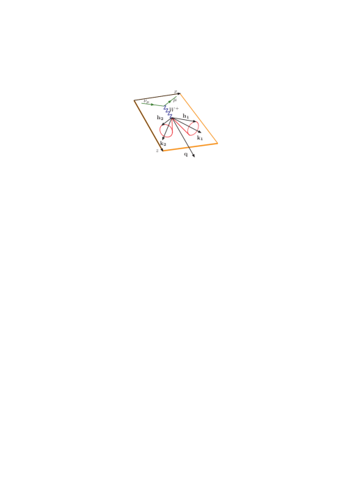
Figure 1: Geometry defining the lepton scattering plane and the two cones spanning the possible momenta of the two holes around the momenta transferred to each nucleon, ${\bf k}_{i}$. The cones are determined by the energy transferred $\omega_{i}$ to each nucleon and by the average hole momenta, $h_{i}$. The final momenta ${\bf p}^{\prime}_{i}={\bf h}_{i}+{\bf k}_{i}$ are not shown for simplicity.

For the total determination of the averaged momenta, ${\bf h}_{i}$, one should know in addition the azimuthal angles with respect to the ${\bf k}_{i}$ vectors. But from the 1p1h response function $R_{\rm 1p1h}(k_{i},\omega_{i})$ there are not restrictions over the azimuthal angles. Energy-momentum conservation only provides restrictions for the magnitude of the initial momenta and their angles with respect to ${\bf k}_{i}$. For a given angle $\theta_{i}$ between ${\bf h}_{i}$ and ${\bf k}_{i}$, Eq. (54), the vector form of ${\bf h}_{i}$ is

$${\bf h}_{i}=h_{i}(\cos\theta_{i}\widehat{\bf k}_{i}+\sin\theta_{i}{\bf u}_{i}),$$ (55)

where $\widehat{\bf k}_{i}$ is the unit vector in the direction of ${\bf k}_{i}$ and ${\bf u}_{i}$ is an unit vector perpendicular to ${\bf k}_{i}$. The vectors ${\bf h}_{i}$ generate two cones around the ${\bf k}_{i}$ vectors, as depicted in Fig. 1. In our reference frame (see below) the vector ${\bf k}_{i}$ can be considered in the scattering plane, spanned by the $x,z$ directions, as shown in Fig. 1, given by

$${\bf k}_{i}=(k_{i}^{x},0,k_{i}^{z}).$$ (56)

Therefore the general form of the unit vector in the plane perpendicular to ${\bf k}_{i}$ is

$${\bf u}_{i}=\pm\frac{(-k_{i}^{z},\alpha_{i},k_{i}^{x})}{\sqrt{(k_{i}^{z})^{2}+\alpha_{i}^{2}+(k_{i}^{x})^{2}}}\,,$$ (57)

where $\alpha_{i}$ is a real parameter that determines the $y$ component of ${\bf h}_{i}$.

There are no restrictions over the values of the two parameters $\alpha_{1}$, $\alpha_{2}$. In practice what we do is to choose several options for these parameters guided by simplicity of the calculation. The simplest option is to choose $\alpha_{1}=\alpha_{2}=0$, but any other election is possible. In the results section we compare several options and discuss which is the best one according to the comparison with the full results, and study how the results depend on the values of $\alpha_{i}$.

3.3 MCA Integration limits

To evaluate the MCA expression for the 2p2h responses, Eq. (31), it is convenient to change the integration variable $\theta_{k_{1}}$ (the angle between ${\bf k}_{1}$ and ${\bf q}$) to the magnitude, $k_{2}$, of the momentum transfer to the second nucleon

$$\cos\theta_{k_{1}}\longrightarrow k_{2}=|{\bf q}-{\bf k}_{1}|.$$ (58)

The Jacobian of the transformation gives

$$k_{1}^{2}dk_{1}d\cos\theta_{k_{1}}d\phi_{k_{1}}=\frac{k_{1}k_{2}}{q}dk_{1}dk_{2}d\phi_{k_{1}}.$$ (59)

Due to the azimuthal symmetry of the inclusive response functions, the integration over the angle $\phi_{k_{1}}$ can be reduced to multiplication by $2\pi$ and evaluation of the integrand for $\phi_{k_{1}}=0$, as a particular case. The MCA reduces to a three-dimensional integral given by

$$R^{K}_{\rm 2p2h} = \frac{V}{(2\pi)^{9}}\frac{2\pi m_{N}^{4}}{q}\int^{(k_{1})_{\rm max}}_{0}dk_{1}k_{1}\int^{q+k_{1}}_{|q-k_{1}|}dk_{2}k_{2}$$ (60)

$$\int^{(\omega_{1})_{\rm max}}_{(\omega_{1})_{\rm min}}d\omega_{1}\langle r^{K}\rangle R_{\rm 1p1h}(k_{1},\omega_{1})R_{\rm 1p1h}(k_{2},\omega-\omega_{1}).$$

1. 

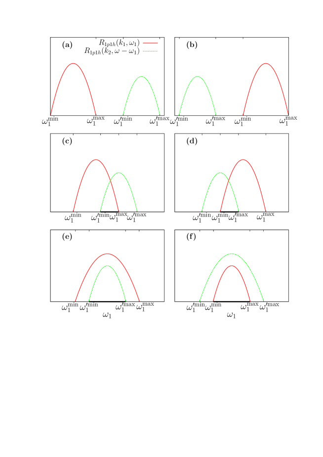
   Figure 2: Graphs of the two $1p1h$ response functions $R_{\rm 1p1h}(k_{1},\omega_{1})$ and $R_{\rm 1p1h}(k_{2},\omega-\omega_{1})$ appearing inside the MCA integral as a function of $\omega_{1}$. The six possible configurations are shown. In cases a, b they do not overlap. In cases c, d they overlap, and finally, in cases e, f, one domain is inside the domain of the other one.

2. To obtain the maximum value of $k_{1}$ we first take into account that the maximum energy allowed for particle no. 1 is

   $$E^{\prime}_{1}\leq\omega+E_{F}$$ (61)

   i.e., all the energy is transferred to particle no. 1, initially with $h_{1}=k_{F}$. The corresponding maximum momentum for this on shell particle is

   $$p^{\prime}_{1}\leq\sqrt{(\omega+E_{F})^{2}-m_{N}^{2}}.$$ (62)

   Therefore the momentum transfer to the first particle is bound from above by

   $$k_{1}=|{\bf p}^{\prime}_{1}-{\bf h}_{1}|\leq p^{\prime}_{1}+h_{1}$$ (63)

   and

   $$(k_{1})_{\rm max}=\sqrt{(\omega+E_{F})^{2}-m_{N}^{2}}+k_{F}.$$ (64)

3. Taking into account the fact that the 1p1h elementary response functions $R_{\rm 1p1h}(k_{i},\omega_{i})=0$ for $\omega_{i}>k_{i}$, we can restrict the integration over $\omega_{1}$ between the limits

   $$(\omega_{1})_{\rm max}=\min(k_{1},\omega),\kern 28.45274pt(\omega_{1})_{\rm min}=\max(0,\omega-k_{2}).$$ (65)

4. For a given value of $k_{i}$, there is an additional restriction for the 1p1h responses, which are zero outside the interval allowed by the Pauli principle (see Appendix A for the proof)

   $$\omega_{i}^{\rm min} = \sqrt{(k_{F}-k_{i})^{2}+m_{N}^{2}}-E_{F}\kern 28.45274pt(=0\quad\mbox{if $k_{i}<2k_{F}$})$$

   $$\omega_{i}^{\rm max} = \sqrt{(k_{F}+k_{i})^{2}+m_{N}^{2}}-E_{F}.$$ (66)

   Therefore the integration limits over $\omega_{1}$ in Eq. (60) can be further constrained by taking into account that, inside the integral, two 1p1h response functions are being multiplied, and both of them must be different from zero simultaneously to contribute. The first response function $R_{\rm 1p1h}(k_{1},\omega_{1})$ is different from zero if

   $$\omega_{1}^{\rm min}<\omega_{1}<\omega_{1}^{\rm max}.$$ (67)

   On the other hand, $R_{\rm 1p1h}(k_{2},\omega-\omega_{1})$ is different from zero if

   $$\omega^{\prime}_{1}{}^{\rm min}<\omega_{1}<\omega^{\prime}_{1}{}^{\rm max}\,,$$ (68)

   where

   $$\omega^{\prime}_{1}{}^{\rm min}=\omega-\omega_{2}{}^{\rm max}$$ (69)

   $$\omega^{\prime}_{1}{}^{\rm max}=\omega-\omega_{2}{}^{\rm min}\,.$$ (70)

   The intersection of the two above intervals defines the final integration range. This is determined by identifying the six different possibilities shown in Fig. 2. In the figure we show with thick lines the resulting integration interval, which depends on the values of $k_{1},k_{2}$ and $\omega$.

4 Electroweak meson-exchange currents

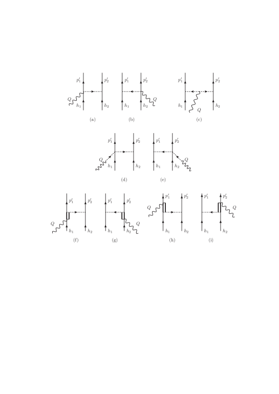
Figure 3: Feynman diagrams for the electroweak MEC model used in this work.

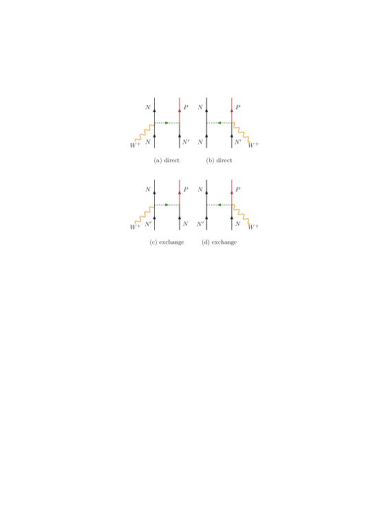
Figure 4: Feynman diagrams for neutron-proton emission with the seagull current.

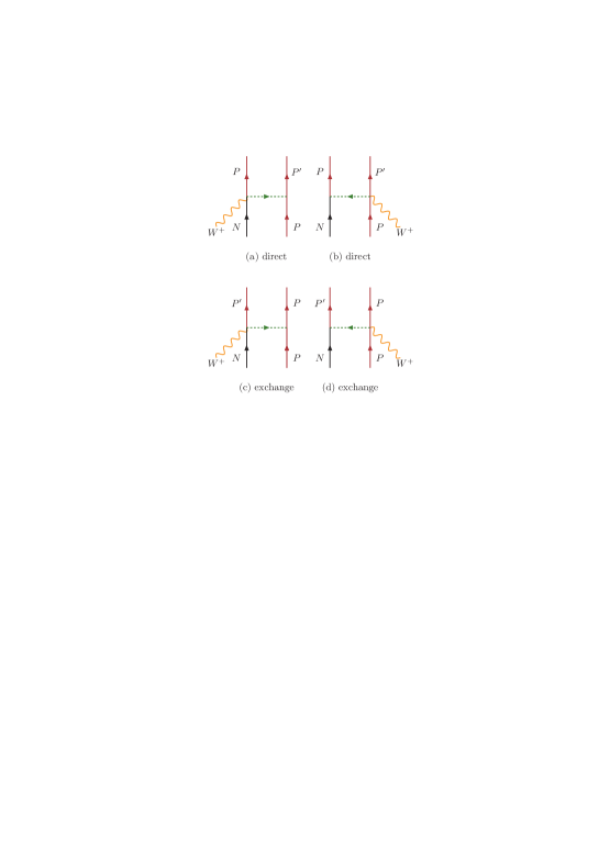
Figure 5: Feynman diagrams for proton-proton emission with the seagull current.

In this section we specify a model for the two-body current matrix elements $j^{\mu}(1^{\prime},2^{\prime},1,2)$ entering in the elementary 2p2h hadronic tensor, Eq. (LABEL:elementary). This will allow us to investigate the validity of the MCA, by comparing to the full integration, following the lines of [46, 39]. The MEC model contains the Feynman diagrams depicted in Fig. 3. The different contributions have been taken from the pion production model of [49]. Our MEC is given as the sum of four two-body currents: seagull (diagrams a,b), pion in flight (c), pion-pole (d,e) and $\Delta(1232)$ excitation (f,g,h,i). Their expressions are given by

$$j^{\mu}_{\rm sea} = \left[I_{V}^{\pm}\right]_{1^{\prime}2^{\prime},12}\frac{f^{2}}{m^{2}_{\pi}}V_{\pi NN}^{s^{\prime}_{1}s_{1}}({\bf p}^{\prime}_{1},{\bf h}_{1})$$ (71)

$$\times \bar{u}_{s^{\prime}_{2}}({\bf p}^{\prime}_{2})\left[F^{V}_{1}(Q^{2})\gamma_{5}\gamma^{\mu}+\frac{F_{\rho}\left(k_{2}^{2}\right)}{g_{A}}\,\gamma^{\mu}\right]u_{s_{2}}({\bf h}_{2})+(1\leftrightarrow 2)\,$$

$$j^{\mu}_{\pi} = \left[I_{V}^{\pm}\right]_{1^{\prime}2^{\prime},12}\frac{f^{2}}{m^{2}_{\pi}}F^{V}_{1}(Q^{2})V_{\pi NN}^{s^{\prime}_{1}s_{1}}({\bf p}^{\prime}_{1},{\bf h}_{1})V_{\pi NN}^{s^{\prime}_{2}s_{2}}({\bf p}^{\prime}_{2},{\bf h}_{2})\left(k^{\mu}_{1}-k^{\mu}_{2}\right)$$ (72)

$$j^{\mu}_{\rm pole} = \left[I_{V}^{\pm}\right]_{1^{\prime}2^{\prime},12}\frac{f^{2}}{m^{2}_{\pi}}\,\frac{F_{\rho}\left(k_{1}^{2}\right)}{g_{A}}\frac{Q^{\mu}\bar{u}_{s^{\prime}_{1}}({\bf p}^{\prime}_{1})\not{\!Q}u_{s_{1}}({\bf h}_{1})}{Q^{2}-m^{2}_{\pi}}V_{\pi NN}^{s^{\prime}_{2}s_{2}}({\bf p}^{\prime}_{2},{\bf h}_{2})$$ (73)

$$+(1\leftrightarrow 2)$$

$$j^{\mu}_{\Delta} = \frac{f^{*}f}{m^{2}_{\pi}}\,V_{\pi NN}^{s^{\prime}_{2}s_{2}}({\bf p}^{\prime}_{2},{\bf h}_{2})\bar{u}_{s^{\prime}_{1}}({\bf p}^{\prime}_{1})\left\{\left[U_{\rm F}^{\pm}\right]_{1^{\prime}2^{\prime},12}k^{\alpha}_{2}G_{\alpha\beta}(h_{1}+Q)\Gamma^{\beta\mu}(h_{1},Q)\right.$$ (74)

$$+\left.\left[U_{\rm B}^{\pm}\right]_{1^{\prime}2^{\prime},12}\;k^{\beta}_{2}\hat{\Gamma}^{\mu\alpha}(p^{\prime}_{1},Q)G_{\alpha\beta}(p^{\prime}_{1}-Q)\right\}u_{s_{1}}({\bf h}_{1})+(1\leftrightarrow 2).$$

In these equations we have introduced the $\pi NN$ vertex function and the pion propagator into the definition of the following spin-dependent function:

$$V_{\pi NN}^{s^{\prime}_{1}s_{1}}({\bf p}^{\prime}_{1},{\bf h}_{1})\equiv\frac{\bar{u}_{s^{\prime}_{1}}({\bf p}^{\prime}_{1})\,\gamma_{5}\not{\!k}_{1}\,u_{s_{1}}({\bf h}_{1})}{k^{2}_{1}-m^{2}_{\pi}}.$$ (75)

We have also defined the following two-particle isospin operators

$$I_{V}^{\pm} = (I_{V})_{x}\pm i(I_{V})_{y}$$ (76)

$$\mbox{\boldmath$I$}_{V} = i\left[\mbox{\boldmath$\tau$}(1)\times\mbox{\boldmath$\tau$}(2)\right],$$ (77)

where the $+(-)$ sign refers to neutrino (antineutrino) scattering. The forward, $U_{\rm F}^{\pm}=U_{Fx}\pm iU_{Fy}$, and backward, $U_{\rm B}^{\pm}=U_{Bx}\pm iU_{By}$, isospin transition operators are obtained from the Cartesian components defined by

$$U_{\rm Fj} = \sqrt{\frac{3}{2}}\sum_{i}\left(T_{i}T_{j}^{\dagger}\right)\otimes\tau_{i}$$ (78)

$$U_{\rm Bj} = \sqrt{\frac{3}{2}}\sum_{i}\left(T_{j}\,T^{\dagger}_{i}\right)\otimes\tau_{i},$$ (79)

where $\vec{T}$ is an isovector transition operator from isospin $\frac{3}{2}$ to $\frac{1}{2}$.

In Figs. 4 and 5 we show the charge-dependent Feynman diagrams contributing to the np and pp emission channels of CC neutrino scattering in the case of the seagull current as an example. They involve direct and exchange contributions. Each current operator contributes analogously. These figures illustrate the complexity of the elementary 2p2h responses $r^{K}$, which here are computed numerically.

We use the $\pi NN$ ($f=1$) and axial ($g_{A}=1.26$) coupling constants. The electroweak form factors $F_{1}^{V}$ and $F_{\rho}$ in the seagull and pionic currents are those of the pion production amplitudes of [49]. Finally, we use the $\pi N\Delta$ coupling constant $f^{*}=2.13$. We also apply strong form factors (not written explicitly in the MEC) of dipole form in all the $NN\pi$ and $N\Delta\pi$ vertices.

For simplicity in this work we only include the dominant terms in the weak $N\rightarrow\Delta$ transition vertex tensor in the forward current, $\Gamma^{\beta\mu}(P,Q)$

$$\Gamma^{\beta\mu}(P,Q)=\frac{C^{V}_{3}}{m_{N}}\left(g^{\beta\mu}\not{\!Q}-Q^{\beta}\gamma^{\mu}\right)\gamma_{5}+C^{A}_{5}g^{\beta\mu}.$$ (80)

We have kept only the $C_{3}^{V}$ and $C_{5}^{A}$ form factors and neglected the smaller contributions of the others. They are taken from [49]. On the other hand, for the backward current, the vertex tensor is

$$\hat{\Gamma}^{\mu\alpha}(P^{\prime},Q)=\gamma^{0}\left[\Gamma^{\alpha\mu}(P^{\prime},-Q)\right]^{\dagger}\gamma^{0}\,.$$ (81)

Finally the $\Delta$-propagator takes into account the finite decay width of the $\Delta\,(1232)$ by the prescription

$$G_{\alpha\beta}(P)=\frac{{\cal P}_{\alpha\beta}(P)}{P^{2}-M^{2}_{\Delta}+iM_{\Delta}\Gamma_{\Delta}+\frac{\Gamma^{2}_{\Delta}}{4}}\,.$$ (82)

In this work we consider both the real and imaginary parts of the denominator of this propagator. The projector ${\cal P}_{\alpha\beta}(P)$ over spin-$\frac{3}{2}$ on-shell particles is given by

$${\cal P}_{\alpha\beta}(P) = -(\not{\!P}+M_{\Delta})\left[g_{\alpha\beta}-\frac{1}{3}\gamma_{\alpha}\gamma_{\beta}-\frac{2}{3}\frac{P_{\alpha}P_{\beta}}{M^{2}_{\Delta}}\right.$$ (83)

$$+ \left.\frac{1}{3}\frac{P_{\alpha}\gamma_{\beta}-P_{\beta}\gamma_{\alpha}}{M_{\Delta}}\right].$$

We do not take into account possible off-shellness effects in this projector.

5 Treatment of the $\Delta$-propagator

Using an average value for the hole momenta inside the MCA integral will be valid only if the elementary 2p2h response functions depend slowly on ${\bf h}_{1}$ and ${\bf h}_{2}$. This is not the case for the forward $\Delta$ diagram, which presents a sharp maximum due to the pole structure of the $\Delta$ propagator,

$$G_{\Delta}(H+Q)\equiv\frac{1}{(H+Q)^{2}-M^{2}_{\Delta}+iM_{\Delta}\Gamma_{\Delta}+\frac{\Gamma^{2}_{\Delta}}{4}}\,,$$ (84)

where $H^{\mu}=(E_{{\bf h}},{\bf h})$ is the four-momentum of the hole. Taking an average value for the momentum instead of computing the full integral modifies the pole position, and this distorts the shape and strength of the 2p2h $\Delta$ peak. Due to this effect, the present MCA approach is not as accurate as in the low-energy region far from the $\Delta$ peak. In this work we compare the results of different methods to improve the description of the $\Delta$ peak:

1. the full $\Delta$ propagator, Eq. (84), but using the corresponding average momentum;

2. the Fermi-averaged or frozen $\Delta$ propagator;

3. the cone-averaged $\Delta$ propagator.

These averaged propagators are explained below.

5.1 The frozen $\Delta$ propagator

This is a propagator averaged over the momentum distribution of the Fermi gas. This produces a smearing of the $\Delta$ peak. This was proven to be an excellent approximation in the case of the frozen approximation of [42], where the momentum of the hole was approximated by zero. Therefore this choice amounts to compute the average integral, by taking the non-relativistic limit for the energies of the hole ($E_{{\bf h}}\simeq m_{N}$),

$$G_{\rm frozen}(Q) = \frac{1}{\frac{4}{3}\pi k^{3}_{F}}\int\frac{d^{3}h\;\theta(k_{F}-\left|{\bf h}\right|)}{a-2\,{\bf h}\cdot{\bf q}+ib}\,,$$ (85)

$$= \frac{1}{\frac{4}{3}\pi k^{3}_{F}}\frac{\pi}{q}\left\{\frac{\left(a+ib\right)k_{F}}{2q}\right.$$

$$\kern-28.45274pt\mbox{}+\left.\frac{4q^{2}k^{2}_{F}-(a+ib)^{2}}{8q^{2}}\ln\left[\frac{a+2k_{F}q+ib}{a-2k_{F}q+ib}\right]\right\}\,,$$

where the parameters $a,b$ are defined by

$$\kern-22.76228pta \equiv m^{2}_{N}+Q^{2}+2m_{N}(\omega+\Sigma)-M^{2}_{\Delta}+\frac{\Gamma^{2}}{4}$$ (87)

$$\kern-22.76228ptb \equiv M_{\Delta}\Gamma\,.$$ (88)

They depend on two parameters, $\Gamma$ and $\Sigma$, that correspond to an effective width and shift of the smeared $\Delta$ peak. These parameters are adjusted to reproduce the full results with the 7D integral, and depend on the momentum transfer $q$. They are given in Table 1. Note that $\Gamma$ is slightly different from the values fitted in [42]. The latter is because in this fit we use the MCA instead of the frozen approximation used in [42].

$q$ (MeV/c)	$\Sigma$ (MeV)	$\Gamma$ (MeV)	$\Gamma_{c}$ (MeV)
300	20	110	145
400	65	135	138
500	65	125	134
800	80	100	128
1000	100	80	125
1200	115	60	123
1500	150	20	120
2000	150	0	105

Table 1: Values of the free parameters of the Fermi-averaged $\Delta$-propagator for different values of the momentum transfer $q$.

Figure 6: Scheme defining the geometry for the cone-averaged integration of the $\Delta$ propagator. The $z^{\prime}$ axis is defined by the direction of the partial momentum transfer ${\bf k}$ to the hole ${\bf h}$. The modulus $h$ and cone angle $\theta$ are fixed by the kinematics of the 1p1h response. The azimuthal angle $\phi$ is undetermined and is integrated around the $z^{\prime}$ axis for the average. The result depends on the cone geometry and on the angle $\theta_{q}$ between ${\bf k}$ and the momentum transfer ${\bf q}$ as well.

5.2 Cone-averaged $\Delta$-propagator

In the present MCA approach the moduli of the momenta $h_{i}$, and the angles $\theta_{i}$ between ${\bf h}_{i}$ and ${\bf k}_{i}$ are fixed, and therefore the vectors ${\bf h}_{i}$ belong to the cones shown in Fig. 1. However the azimuthal angles in the cones are not determined, and here we choose different prescriptions to fix them. By doing that, the $\Delta$-peak position is altered with respect to the exact value obtained in the full 7D integral. The cone-averaged propagator introduced here is defined by smearing the $\Delta$ propagator by averaging only in the cone instead of averaging over the full Fermi sea:

$$G_{\Delta}(H+Q)\rightarrow G_{\rm cone}\equiv\frac{1}{2\pi}\int\frac{d\phi}{a_{c}-2\,{\bf h}\cdot{\bf q}+ib_{c}}\,,$$ (89)

where the integration variable $\phi$ is the azimuthal angle around the cone shown in Fig. 6, ${\bf k}$ is the partial momentum transfer to the hole ${\bf h}$ and ${\bf q}$ is the total momentum transfer. The cone-averaged propagator depends on the parameters in the denominator, $a_{c},b_{c}$, defined by

$$\kern-22.76228pta_{c} \equiv m^{2}_{N}+Q^{2}+2E_{h}\omega-M^{2}_{\Delta}+\frac{\Gamma_{c}^{2}}{4}$$ (90)

$$\kern-22.76228ptb_{c} \equiv M_{\Delta}\Gamma_{c}\,.$$ (91)

These cone parameters are independent of $\phi$. The $\phi$ dependence is hidden in the scalar product ${\bf h}\cdot{\bf q}$. To obtain this dependence we use Fig. 6 in the rotated coordinate system, $x^{\prime}z^{\prime}$, in the scattering plane, where the $z^{\prime}$ axis points along ${\bf k}$. In this system the scalar product is

$${\bf h}\cdot{\bf q}=hq(\sin\theta\sin\theta_{q}\cos\phi+\cos\theta\cos\theta_{q})\,,$$ (92)

where $\theta$ is the angle between ${\bf h}$ and ${\bf k}$, defining the cone, and $\theta_{q}$ is the angle between ${\bf k}$ and ${\bf q}$. The cone-averaged propagator can be expressed as the integral

$$G_{\rm cone}=\frac{1}{2\pi}\int\frac{d\phi}{W-C\cos\phi}\,,$$ (93)

with

$$W = a_{c}+ib_{c}-hq\cos\theta\cos\theta_{q}$$ (94)

$$C = hq\sin\theta\sin\theta_{q}.$$ (95)

Note that $C>0$ and $W$ is a complex number. The above integral is performed analytically in Appendix B.

The values of the effective width in the cone-averaged propagator, $\Gamma_{c}$, are tabulated as a function of $q$ in Table 1.

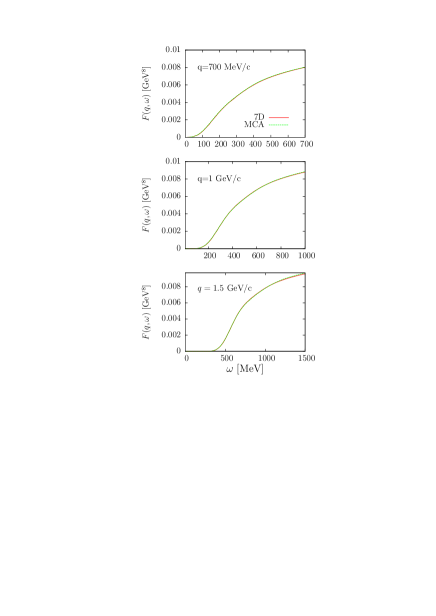
Figure 7: Phase space function computed for three values of the momentum transfer, as a function of $\omega$. Results obtained with the full 7D integral are compared to the MCA approach with only 3D integrations.

6 Results

In this section we present results for the 2p2h response functions for inclusive neutrino scattering. In this work we do not provide comparisons with the experimental data. This requires one to describe simultaneously the quasielastic and inelastic (including pion emission) channels. In previous works [38, 40] we have provided this comparison within the superscaling approach plus a MEC model derived from the one used in the present work. This model describes the $(e,e^{\prime})$ cross section of ¹²C and the global set of neutrino scattering quasielastic without pions (CC0$\pi$) measurements made in the neutrino accelerator experiments. Therefore the model we are starting with is realistic for describing two-nucleon emission with neutrinos for the kinematics of interest.

In particular we investigate the validity of the MCA approach presented so far, by evaluating the 2p2h response functions and comparing with the full results obtained with the 7D integration. The interest of this investigation is to determine the consistency between different approaches to the 2p2h emission channel, namely the model of [6, 10]. This is a first step towards the reconciliation between apparently different approaches. This study is a necessary step forward in reducing the systematic errors in the oscillation parameters coming from the theoretical uncertainties. Moreover it is interesting by itself to find alternative approximations that allow a reduction of the computational time of the two-nucleon emission without large loss of numerical precision. Finally we remark that the MCA allows us to make an easier connection between our results and the predictions provided by other authors [6].

We consider the case of the nucleus ¹²C, and, unless otherwise stated, the Fermi momentum is chosen to be $k_{F}=228$ MeV/c. We show results for several kinematics in the range of momentum transfer between 300 MeV/c and 2 GeV/c, of interest for the neutrino oscillation experiments.

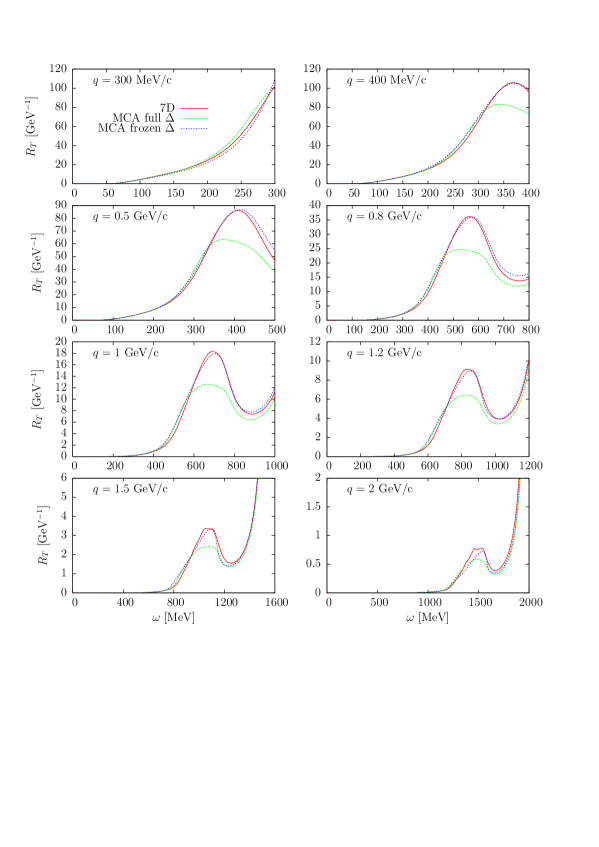
Figure 8: Transverse 2p2h response function as a function of $\omega$ for several values of the momentum transfer. The results of the RFG with the full 7D integration are compared to the MCA with the full $\Delta$ propagator and with the Fermi-averaged or frozen $\Delta$ propagator.

We start by computing the phase-space function obtained from Eq. (21) for $r^{K}=1$, except for a constant factor. This is a universal function for the RFG that only depends on the kinematics of the 2p2h excitations and not on the MEC model:

$$F(q,\omega) = \int d^{3}p^{\prime}_{1}d^{3}h_{1}d^{3}h_{2}\frac{m_{N}^{4}}{E_{1}E_{2}E^{\prime}_{1}E^{\prime}_{2}}\Theta(p^{\prime}_{1},h_{1})\Theta(p^{\prime}_{2},h_{2})$$ (96)

$$\delta(E^{\prime}_{1}+E^{\prime}_{2}-E_{1}-E_{2}-\omega).$$

This universal function is well established and was fully studied in [46, 47]. Therefore the comparison with this function is a required consistency check in any calculation of the 2p2h response, and furthermore it provides a valuable precision check of the multidimensional integrations. In fact the phase space determines the global behavior of the 2p2h responses, on top of the additional modifications introduced by the particular model of two-body current operator. The main one is produced by the $Q^{2}$ dependence of the electromagnetic form factors and the structure of the different diagrams, which are dominated by the forward $\Delta$ excitations. The remaining $(q,\omega)$ dependence of the MEC diagrams is found to be smoother.

The results in Fig. 7 confirm numerically that the MCA approach treats exactly the phase space in all energy regions, obtaining essentially the same results except for numerical errors in the integration procedure. This comparison also allows us to determine the optimal integration steps in the MCA.

In Fig. 8 we compare the transverse 2p2h response function of the RFG computed by performing the full 7D integration with the MCA results for two different prescriptions for the $\Delta$ propagator. Using the full $\Delta$ propagator in the MCA produces a peak that is about $30\%$ smaller than the full result, and slightly shifted and distorted. This is due to the approximation made for the averaged momentum of the hole, and to the chosen values of the azimuthal angles in the cones shown in Fig. 1. These results have been obtained for $\alpha_{1}=\alpha_{2}=0$, corresponding to both holes contained in the scattering plane on the same side of the cone, and corresponding to choosing the $+$ sign in Eq. (57). Therefore the position and the value of the maximum due to the forward $\Delta$ propagator is altered by the average in the MCA. This problem is dealt with in this example by using the smeared frozen $\Delta$ propagator averaged over the RFG momentum distribution, as also shown in Fig. 8 with dotted lines, which are quite similar to the full results, after fitting the two parameters of the effective width and shift, $(\Gamma,\Sigma)$, shown in Table 1. Note that for low transferred energy, far from the resonance position, and especially at threshold, all the results coincide independently of the $\Delta$-propagator treatment. Thus, globally, the MCA results using the frozen $\Delta$ propagator are quite satisfactory.

Nonetheless the quality of the agreement relies on using the fitted values for the width and shift, which depend strongly on $q$. However, notice that this procedure may limit the predictability of the present approach in so far as its reliability is linked to the knowledge of the full results.

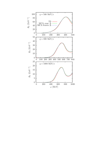
Figure 9: Transverse 2p2h response function as a function of $\omega$ for several values of the momentum transfer. The results of the RFG with the full 7D integration are compared to the MCA with the cone averaged $\Delta$ propagator and with the frozen $\Delta$ propagator.

An alternative solution is to use the cone-averaged propagator, which only depends on one parameter $\Gamma_{c}$ with a milder dependence on $q$, as shown in Table 1, which oscillates between 145 and 105 MeV in the $q$ range considered, more or less around the free $\Delta$ width, $\Gamma_{c}=125\pm 20$. On the other hand, the frozen width $\Gamma$ changes in the larger range between 135 and zero. Results with the cone-averaged $\Delta$ propagator are shown in Fig. 9. They are similar to the exact results and the quality of this approximation is at least as good as using the frozen $\Delta$ propagator. However the cone-averaged approximation has the advantage of having only one free parameter, the $\Gamma_{c}$ width, which is also closer to the $\Delta$ free width. The agreement with the full results is remarkable in the full range of momentum transfer explored in this work.

From now on all the results of the MCA shown will be calculated using the cone-averaged $\Delta$ propagator, with the parameters displayed in the last column of Table 1.

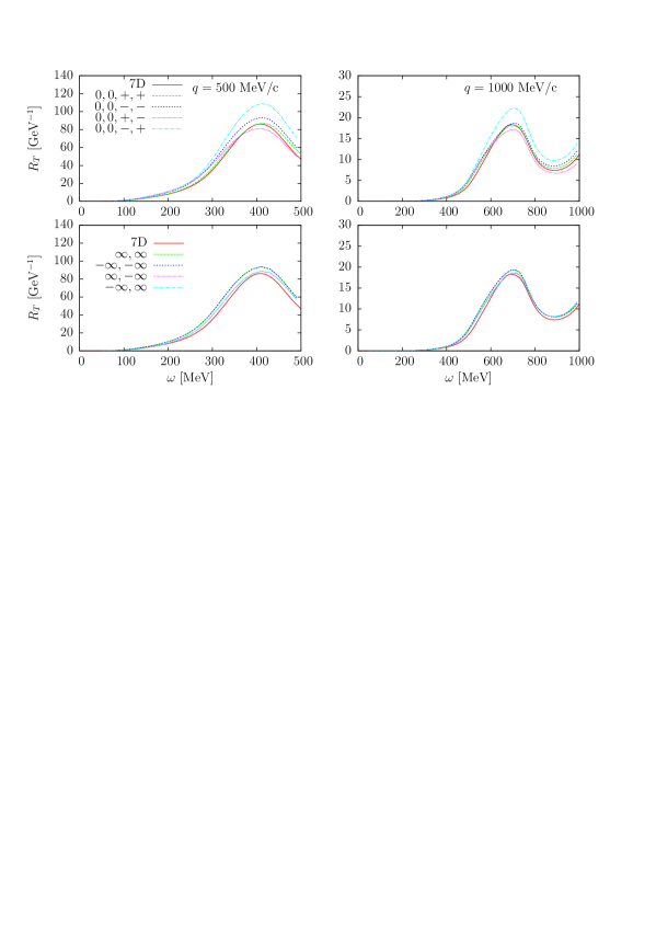
Figure 10: 2p2h transverse response function plotted against transferred energy, $\omega$, for different $q$-values ($q=500$ MeV/c on the left side and $q=1000$ MeV/c on the right one) and for different average momenta orientations, labelled by the keys defined in Fig. 11.

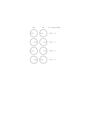
(a) Configurations for initial holes’ momenta on the scattering plane, labelled by the key indicating their ($\alpha_{1},\alpha_{2}$) values and their signs corresponding to Eq. (57).

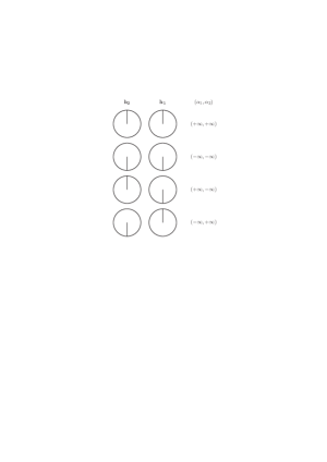
(b) Configurations for initial holes’ momenta out of the scattering plane, labelled by the key indicating their ($\alpha_{1},\alpha_{2}$) values and their signs corresponding to Eq. (57).

Figure 11: Different initial holes’ configurations considered in this work.

In Fig. 10 we study the dependence of the MCA results on the chosen value for the azimuthal angles of the initial hole momenta. As was shown in Fig. 1, each averaged momentum ${\bf h}_{i}$ is arranged in the lateral surface of the corresponding cone depicted in the figure. The precise value of the azimuthal angle measured with respect to ${\bf k}_{i}$ (the cone axis) is determined by the parameters $\alpha_{i}$ in Eq. (57) and the sign of the unit vector ${\bf u}_{i}$. Any combination of pairs of azimuthal angles between 0 and $2\pi$ is possible. In Fig. 10 we show different pairs of choices and compare the corresponding $T$ responses. In Fig. 11 we show the configurations chosen for this study, viewed from the cone bases. In the (a) case the two holes are in the scattering plane but we change their positions among the two possible sides of the cones, corresponding to $\alpha_{i}=0$, and sign $\pm$ for ${\bf u}_{i}$. In the (b) case the hole momenta are out of the scattering plane with the maximum angle allowed, corresponding to $\alpha_{i}=\pm\infty$. As we see, the results depend mildly on the different choices, and we can identify configurations which are particularly stable with little dependence on the chosen values. In particular, the MCA results computed for $\alpha_{i}=\pm\infty$ are all quite similar to the full 7D response function, all of them being in an interval around $\sim 5\%$ above the full result. The same can be said for the $(0,0,-,-)$ configuration, while the worst results occur for $(0,0,-,+)$. This is related to the fact that we are constraining the two ${\bf h}_{i}$ momenta to be the closest to the momentum transfer ${\bf q}$, as can be seen in Fig. 11. This restricts the possible arrangements of the hole pairs in the average momenta approximation. We conclude that the maximum uncertainty of the MCA methods comes from this choice. Note that of all these configurations, only the case $(0,0,+,+)$ was fitted to the full response, while the others are not fitted, and are computed with $\Gamma_{c}$ parameter fixed to this case.

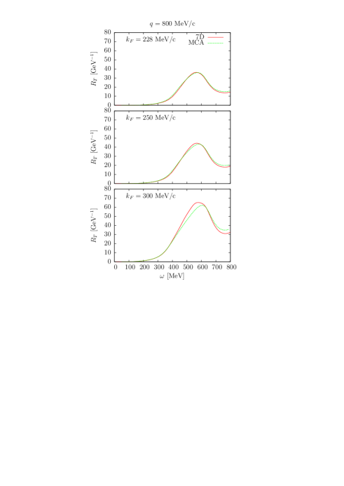
Figure 12: 2p2h transverse response function of ¹²C, for $q=800$ MeV/c, plotted against $\omega$, for different values of the Fermi momentum $k_{F}$.

In Fig. 12 we show an example of how the present MCA results behave when the value of the Fermi momentum is changed. Note that in all cases the nucleus considered is ¹²C, but the Fermi momentum is increased up to $k_{F}=300$ MeV. In a different nucleus, these results should be rescaled with the number of particles in addition to the increase observed in the figure when $k_{F}$ is enlarged. In fact the $R_{T}$ 2p2h response per nucleon is almost a factor of two when $k_{F}$ changes from 228 to 300 MeV/c. More precisely, the ratio between the maxima of the two responses is about 1.75, in agreement with the results of [50], where it was shown that the 2p2h response functions scale as $k_{F}^{2}$. As we see the MCA results are quite stable in this range of $k_{F}$, yet the parameter $\Gamma_{c}$ was fitted for one particular $k_{F}=228$ MeV/c. And this is why the results worsen a bit for higher $k_{F}$. These results show that the MCA approach can be applied to heavier nuclei. Although not presented here, the present formalism can be extended with small changes to the case of $N\neq Z$ nuclei, with different Fermi momenta for protons and neutrons. This will allow one to compute the 2p2h cross sections for neutrino scattering from detectors made of different nuclei (typically C, O, Ar) such as the ones used in ongoing neutrino experiments.

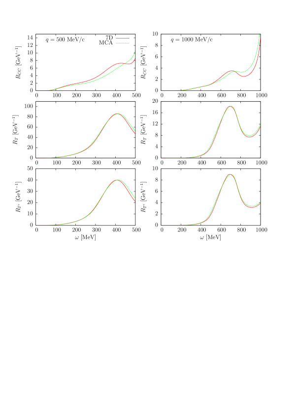
Figure 13: Comparison of the MCA and full results for the $CC$, $T$ and $T^{\prime}$ 2p2h response functions of ¹²C, and for two values of the momentum transfer.

Finally, in Fig. 13 we show that the MCA approach works quite well for the 2p2h response functions of the different kinds, although the parameters have been fitted only for the $T$ response. The worst agreement occurs for the small $R_{CC}$, which partially cancels with the $CL$ and $LL$ responses. The main contribution to neutrino scattering thus comes from the $T$ and $T^{\prime}$ responses, which are well described in the MCA approach.

7 Conclusions

In this work we have introduced a simplified approach, the modified convolution approximation (MCA), which allows one to write the 2p2h response functions as a convolution of two single-particle response functions weighted with the average 2p2h elementary responses. The approach treats exactly the kinematics of the 2p2h excitation and therefore it works the best for low energy transfers. The resulting approximation allows one to reduce the number of integrals from seven to three dimensions, with a considerable saving in computational effort. Our formalism includes the interference between direct and exchange diagrams.

After introducing the general formalism in this approach, we have tested its quality and precision by comparing with the full results using a specific model of relativistic two-body MEC operators. The approach works well when an appropriate smearing of the $\Delta$ propagator, obtained by averaging it over the hole momenta, is used. This approximation requires to choose the specific direction of the average momenta for the initial nucleons in the current matrix elements, which is contained over the surface of a cone. We have found that a simple averaged propagator over the azimuthal angle of the hole momentum around the cone gives quite good results for all the values of the kinematics. The ambiguities in the model related to the prescription for the direction of the hole over the cone surface are found to be mild.

The MCA presented here can also be considered as the natural generalization of the pioneering non-relativistic formalism of [2] to the relativistic case, which requires to add an additional integral over the energy $\omega_{1}$ transferred to the first nucleon.

Furthermore the present approach provides an integral representation of the 2p2h responses which is similar to the model of Valencia [6] and therefore this can yield a comparison of the compatibility with the approach of the Torino model [39]. Moreover getting the 2p2h responses written in terms of two 1p1h response functions (or Lindhard functions) allows us to include a phenomenological scaling function instead of the Lindhard function of the free Fermi gas to evaluate the 2p2h responses. This opens the possibility to extend the free Fermi gas 2p2h response functions to what is expected from an interacting nucleus. In addition, this can be also seen as an alternative way to include finite-size effects in the Fermi gas 2p2h responses instead of the more common local density approximation [29].

8 Acknowledgements

This work has been partially supported by the Spanish Ministerio de Economia y Competitividad and ERDF (European Regional Development Fund) under contracts FIS2014-59386-P, FIS2014-53448-C2-1, by the Junta de Andalucia (grants No. FQM-225, FQM160), by the INFN under project MANYBODY, and part (TWD) by the U.S. Department of Energy under cooperative agreement DE-FC02-94ER40818. IRS acknowledges support from a Juan de la Cierva fellowship from MINECO (Spain). GDM acknowledges support from a Junta de Andalucia fellowship (FQM7632, Proyectos de Excelencia 2011).

Appendix A Boundaries of the 1p1h responses

In this appendix we derive the $\omega$-limits of the RFG response function, Eq. (51).

We use the following result, which is easy to prove and states that if an on-shell particle with momentum $p$ inside the Fermi gas takes energy-momentum $(\omega,q)$, then the limit cases, ${\bf p}$ parallel or anti-parallel to ${\bf q}$, correspond to the condition

$$\left.\begin{array}[]{c}E_{p-q}=E+\omega\\ \mbox{or}\\ E_{p+q}=E+\omega\\ \end{array}\right\}\Leftrightarrow\kappa\sqrt{1+1/\tau}-\lambda=\epsilon.$$ (97)

For fixed $q$, the limits of the quasielastic peak correspond to the scaling variable $\psi^{2}=1$; see Eq. (51).

From the definition of $\psi$, Eq. (49), this corresponds to $\epsilon_{0}=\epsilon_{F}$, that is, a particle with Fermi momentum. In the non-Pauli blocked regime, from Eq. (45), the minimum energy for the particle is exactly $\epsilon$ as given in Eq. (97). This implies that

$$\kappa\sqrt{1+1/\tau}-\lambda=\epsilon_{F}\Leftrightarrow\left\{\begin{array}[]{c}E_{k_{F}-q}=E_{F}+\omega\\ \mbox{or}\\ E_{k_{F}+q}=E_{F}+\omega\\ \end{array}.\right.$$ (98)

From this latter equation, by isolating $\omega$, one obtains the upper and lower $\omega$-limits given in Eq. (66).

Appendix B Cone-averaged propagator

Here the integral appearing in the cone-averaged $\Delta$ propagator is computed

$$I(W,C)\equiv\int_{0}^{2\pi}\frac{d\phi}{W-C\cos\phi}\,,$$ (99)

where $C>0$ and $W$ is a complex number. We transform the integral into a contour integral in the complex plane on the variable $z=e^{i\phi}$. By multiplying and dividing by $z$ inside the integral we obtain

$$I(W,C) = \int_{0}^{2\pi}\frac{e^{i\phi}d\phi}{We^{i\phi}-C\frac{e^{2i\phi}+1}{2}}$$ (100)

$$= 2i\oint\frac{dz}{Cz^{2}-2Wz+C},$$

where the last integral is made along the unit circle counterclockwise. The integral is evaluated by computing the poles inside the circle. The poles are given by the roots of the second degree polynomial in the denominator, written in factorized form as

$$Cz^{2}-2Wz+C=C(z-z_{1})(z-z_{2})$$ (101)

where obviously $z_{1}z_{2}=1$ is satisfied, and

$$z_{1} = \frac{W}{C}+\frac{1}{C}\sqrt{W^{2}-C^{2}}$$ (102)

$$z_{2} = \frac{W}{C}-\frac{1}{C}\sqrt{W^{2}-C^{2}}.$$ (103)

If $z_{1}$ is the pole inside the circle, then $z_{2}$ is automatically outside because $|z_{1}z_{2}|=1$. Therefore there is only one pole inside the circle. The integral is then computed as the residue at the pole

$$I(W,C)=\frac{2i}{C}2\pi i\begin{array}[t]{c}\textstyle\rm Res\\ \scriptstyle|z_{i}|<1\end{array}\frac{1}{(z-z_{1})(z-z_{2})}.$$ (104)

In the case $|z_{1}|<1$, this gives

$$I(W,C)=-\frac{4\pi}{C}\frac{1}{z_{1}-z_{2}}=-\frac{2\pi}{\sqrt{W^{2}-C^{2}}}.$$ (105)

In the other case, $|z_{1}|>1$, the pole inside the circle is $z_{2}$, and the result is

$$I(W,C)=-\frac{4\pi}{C}\frac{1}{z_{2}-z_{1}}=\frac{2\pi}{\sqrt{W^{2}-C^{2}}}.$$ (106)

References

- [1] T. W. Donnelly, J. W. Van Orden, T. De Forest, Jr. and W. C. Hermans, Phys. Lett. 76B (1978) 393.
- [2] J. W. Van Orden and T. W. Donnelly, Ann. Phys. 131 (1981) 451.
- [3] W.M. Alberico, M. Ericson, and A. Molinari, Ann. Phys. 154 (1984) 356.
- [4] M. Martini, M. Ericson, G. Chanfray, J. Marteau, Phys. Rev. C 80 (2009) 065501.
- [5] M. Martini, M. Ericson, G. Chanfray, J. Marteau, Phys. Rev. C 81 (2010) 045502.
- [6] J. Nieves, I. Ruiz Simo, M.J. Vicente Vacas, Phys. Rev. C 83 (2011) 045501.
- [7] J. Nieves, I. Ruiz Simo, M.J. Vicente Vacas, Phys. Lett. B 707 (2012) 72.
- [8] J.E. Amaro, M.B. Barbaro, J.A. Caballero, T.W. Donnelly, C.F. Williamson, Phys. Lett. B 696 (2011) 151.
- [9] J.E. Amaro, M.B. Barbaro, J.A. Caballero, T.W. Donnelly, Phys. Rev. Lett. 108 (2012) 152501.
- [10] R. Gran, J. Nieves, F. Sanchez, M.J. Vicente Vacas, Phys.Rev. D 88 (2013) 113007.
- [11] K. Gallmeister, U. Mosel and J. Weil, Phys. Rev. C 94 (2016) 035502.
- [12] J.T. Sobczyk, Phys. Rev. C 86 (2012) 015504.
- [13] L. Alvarez-Ruso et al., arXiv:1706.03621 [hep-ph].
- [14] U. Mosel, Ann. Rev. Nuc. Part. Sci. 66 (2016) 171.
- [15] T. Katori and M. Martini, arXiv:1611.07770 [hep-ph].
- [16] R. Shneor, et al., (JLab Hall A Collaboration), Phys. Rev. Lett. 99 (2007) 072501.
- [17] R. Subedi, et al., Science 320 (2008) 1476.
- [18] O. Hen et al. [CLAS Collaboration], Phys. Lett. B 722 (2013) 63.
- [19] O. Hen et al. [CLAS Collaboration], Science, 346 (2014) 614.
- [20] J. Ryckebusch, M. Vanhalst, W. Cosyn, J. Phys. G: Nucl. Part. Phys. 42 (2015) 055104.
- [21] C. Colle, O. Hen, W. Cosyn, I. Korover, E. Piasetzky, J. Ryckebusch, and L. B. Weinstein, Phys. Rev. C 92 (2015) 024604.
- [22] C. Colle, W. Cosyn, J. Ryckebusch, Phys. Rev. C 93 (2016) 034608.
- [23] R. Acciarri, et al., Phys. Rev. D 90 (2014) 012008.
- [24] L.B. Weinstein, O. Hen, E. Piasetzky, Phys.Rev. C 94 (2016) 045501.
- [25] K. Niewczas, J. T. Sobczyk, Phys. Rev. C 93 (2016) 035502.
- [26] T. Van Cuyck, N. Jachowicz, R. Gonzalez-Jimenez, M. Martini, V. Pandey, J. Ryckebusch and N. Van Dessel, Phys. Rev. C 94 (2016) 024611.
- [27] T. Van Cuyck, N. Jachowicz, R. Gonzalez-Jimenez, J. Ryckebusch and N. Van Dessel, arXiv:1702.06402 [nucl-th].
- [28] J. E. Amaro, G. Co’, A. M. Lallena, Ann. Phys. 221 (1993) 306.
- [29] J. E. Amaro, A. M. Lallena and G. Co, Nucl. Phys. A 578 (1994) 365.
- [30] W.M. Alberico, A. De Pace, A. Drago, and A. Molinari, Riv. Nuov. Cim. vol. 14, n.5 (1991) 1.
- [31] A. Gil, J. Nieves, and E. Oset, Nucl. Phys. A 627 (1997) 543.
- [32] M.J. Dekker, P.J. Brussaard, and J.A. Tjon, Phys. Lett. B 266 (1991) 249.
- [33] M.J. Dekker, P.J. Brussaard, and J.A. Tjon, Phys. Lett. B 289 (1992) 255.
- [34] M.J. Dekker, P.J. Brussaard, and J.A. Tjon, Phys. Rev. C 49 (1994) 2650.
- [35] A. De Pace, M. Nardi, W. M. Alberico, T. W. Donnelly and A. Molinari, Nucl. Phys. A 726 (2003) 303.
- [36] A. De Pace, M. Nardi, W. M. Alberico, T. W. Donnelly and A. Molinari, Nucl. Phys. A 741 (2004) 249.
- [37] J. E. Amaro, C. Maieron, M. B. Barbaro, J. A. Caballero and T. W. Donnelly, Phys. Rev. C 82 (2010) 044601.
- [38] G. D. Megias, J. E. Amaro, M. B. Barbaro, J. A. Caballero and T. W. Donnelly, Phys. Rev. D 94 (2016) 013012.
- [39] I. Ruiz Simo, J. E. Amaro, M. B. Barbaro, A. De Pace, J. A. Caballero and T. W. Donnelly, J.Phys. G 44 (2017) 065105.
- [40] G. D. Megias, J. E. Amaro, M. B. Barbaro, J. A. Caballero, T. W. Donnelly and I. Ruiz Simo, Phys. Rev. D 94 (2016) 093004.
- [41] R.C. Carrasco and E. Oset, Nucl. Phys. A 536 (1992) 445.
- [42] I. Ruiz Simo, J. E. Amaro, M. B. Barbaro, J. A. Caballero, G. D. Megias and T. W. Donnelly, Phys. Lett. B 770 (2017) 193.
- [43] J.E. Amaro, M.B. Barbaro, J.A. Caballero, T.W. Donnelly A. Molinari, and I. Sick, Phys. Rev. C 71 (2005) 015501.
- [44] J.E. Amaro, M.B. Barbaro, J.A. Caballero, T.W. Donnelly, C. Maieron, Phys. Rev. C 71 (2005) 065501.
- [45] J.E. Amaro, A.M. Lallena, G. Co’, Int. J. Mod. Phys. E 03 (1994) 735.
- [46] I. Ruiz Simo, C. Albertus, J. E. Amaro, M. B. Barbaro, J. A. Caballero and T. W. Donnelly, Phys. Rev. D 90 (2014) 033012.
- [47] I. Ruiz Simo, C. Albertus, J. E. Amaro, M. B. Barbaro, J. A. Caballero and T. W. Donnelly, Phys. Rev. D 90 (2014) 053010.
- [48] J. Nieves, J.E. Amaro, and M. Valverde, Phys. Rev. C 70 (2004) 055503.
- [49] E. Hernandez, J. Nieves and M. Valverde, Phys. Rev. D 76 (2007) 033005.
- [50] J. E. Amaro, M. B. Barbaro, J. A. Caballero, A. De Pace, T. W. Donnelly, G. D. Megias and I. Ruiz Simo, Phys.Rev. C95 (2017) no.6, 065502.