Relativistic Collisions as Yang–Baxter maps

Abstract

We prove that one-dimensional elastic relativistic collisions satisfy the set-theoretical Yang–Baxter equation. The corresponding collision maps are symplectic and admit a Lax representation. Furthermore, they can be considered as reductions of a higher dimensional integrable Yang–Baxter map on an invariant manifold. In this framework, we study the integrability of transfer maps that represent particular periodic sequences of collisions.

1 Introduction to Yang–Baxter maps

Solutions of the set-theoretical Yang–Baxter equation [3, 4, 6, 22, 24, 26, 27], as well as their applications have been extensively studied from various perspectives of mathematics and physics. We will use the short term “Yang–Baxter maps” for these solutions which was introduced in [24]. Namely, for a set $\mathcal{X}$ a Yang–Baxter (YB) map is a map $R:\mathcal{X}\times\mathcal{X}\rightarrow\mathcal{X}\times\mathcal{X}$, $R:(x,y)\mapsto(u(x,y),v(x,y))$, that satisfies the YB equation

$$R_{23}\circ R_{13}\circ R_{12}=R_{12}\circ R_{13}\circ R_{23}.$$

Here, by $R_{ij}$ for $i,j=1,2,3$, we denote the action of the map $R$ on the $i$ and $j$ factor of $\mathcal{X}\times\mathcal{X}\times\mathcal{X}$, i.e. $R_{12}(x,y,z)=(u(x,y),v(x,y),z)$, $R_{13}(x,y,z)=(u(x,z),y,v(x,z))$ and $R_{23}(x,y,z)=(x,u(y,z),v(y,z))$. Moreover, $R$ is called quadrirational if both maps $u(\cdot,y)$, $v(x,\cdot)$, for fixed $y$ and $x$ respectively, are birational isomorphisms of $\mathcal{X}$ to itself.

Parametric versions of YB maps are closely related to integrable quadrilateral equations which constitute discrete analogue of partial differential equations (see e.g. [7, 11, 14, 15, 16]). In these cases the YB property reflects the 3-dimensional (3D) consistency property of the corresponding equation. Parametric YB maps [24, 25] involve two parameters in a parameter space $\mathcal{I}$ that can be considered as extra variables invariant under the map. Particularly, a parametric YB map is a YB map $R:(\mathcal{X}\times\mathcal{I})\times(\mathcal{X}\times\mathcal{I})\mapsto(\mathcal{X}\times\mathcal{I})\times(\mathcal{X}\times\mathcal{I})$, with

$$R:((x,\alpha),(y,\beta))\mapsto((u,\alpha),(v,\beta))=((u(x,\alpha,y,\beta),\alpha),(v(x,\alpha,y,\beta),\beta)).$$ (1)

We usually keep the parameters separate and denote the map (1) just by $R_{\alpha,\beta}(x,y):\mathcal{X}\times\mathcal{X}\rightarrow\mathcal{X}\times\mathcal{X}$. A classification of parametric YB maps on $\mathbb{CP}^{1}\times\mathbb{CP}^{1}$ has been achieved in [2, 17]. According to [23], a Lax matrix of the parametric YB map (1) is a matrix $L$ that depends on a point $x\in\mathcal{X}$, a parameter $\alpha\in\mathcal{I}$ and a spectral parameter $\zeta\in\mathbb{C}$, such that

$$L(u,\alpha,\zeta)L(v,\beta,\zeta)=L(y,\beta,\zeta)L(x,\alpha,\zeta).$$ (2)

Moreover, we call $L$ a strong Lax matrix if equation (2) is equivalent to $(u,v)=R_{\alpha,\beta}(x,y)$. On the other hand, if $u=u_{\alpha,\beta}(x,y),v=v_{\alpha,\beta}(x,y)$ satisfy (2) for a matrix $L$ and the equation

$$L(\hat{x},\alpha,\zeta)L(\hat{y},\beta,\zeta)L(\hat{z},\gamma,\zeta)=L(x,\alpha,\zeta)L(y,\beta,\zeta)L(z,\gamma,\zeta)$$

implies that $\hat{x}=x,\ \hat{y}=y$ and $\hat{z}=z$ for every $x,y,z\in\mathcal{X}$, then $R_{\alpha,\beta}(x,y)\mapsto(u,v)$ is a parametric YB map with Lax matrix $L$ [8, 24].

The integrability aspects of YB maps have been studied by Veselov [24, 25]. It was shown that for any YB map there is a hierarchy of commuting transfer maps. From the corresponding Lax representation of the original YB map a monodromy matrix is defined, whose spectrum is preserved under the transfer maps. In many cases of multidimensional YB maps with polynomial Lax matrices, r-matrix Poisson structures provide the right framework to study the integrability of the transfer maps [8, 10].

2 One-dimensional elastic collisions as YB maps

The one dimensional non-relativistic elastic collision of two particles with masses $m_{1}$ and $m_{2}$ is described by

$$v_{1}^{\prime}=\frac{v_{1}(m_{1}-m_{2})+2m_{2}v_{2}}{m_{1}+m_{2}},\ v_{2}^{\prime}=\frac{v_{2}(m_{2}-m_{1})+2m_{1}v_{1}}{m_{1}+m_{2}},$$

where $v_{1}$, $v_{2}$ are the initial velocities and $v_{1}^{\prime}$, $v_{2}^{\prime}$ the velocities after the collision. A simple calculation shows that the linear map $R^{0}_{m_{1},m_{2}}(v_{1},v_{2})=(v_{1}^{\prime},v_{2}^{\prime})$ is a parametric YB map. In this case, the corresponding transfer maps are linear and their dynamical behavior quite simple.

The relativistic case is much more interesting. In this case, the conservation of relativistic energy and momentum is expressed as

$$m_{1}c^{2}\gamma(v_{1})+m_{2}c^{2}\gamma(v_{2}) = m_{1}c^{2}\gamma(v_{1}^{\prime})+m_{2}c^{2}\gamma(v_{2}^{\prime}),$$ (3)

$$m_{1}v_{1}\gamma(v_{1})+m_{2}v_{2}\gamma(v_{2}) = m_{1}v_{1}^{\prime}\gamma(v_{1}^{\prime})+m_{2}v_{2}\gamma(v_{2}^{\prime}),$$ (4)

where $\gamma$ denotes the Lorentz factor $\gamma(v)=\frac{1}{\sqrt{1-v^{2}/c^{2}}}$ (we will always assume $|v_{i}|<c$). The velocities $v_{1}^{\prime},v_{2}^{\prime}$ after collision are given in terms of the initial velocities $v_{1},v_{2}$ by solving (3)-(4). From this solution (excluding the trivial solution $v_{1}^{\prime}=v_{1},v_{2}^{\prime}=v_{2}$) we define the collision map

$$\mathcal{R}_{m_{1},m_{2}}:(v_{1},v_{2})\mapsto(v_{1}^{\prime},v_{2}^{\prime}).$$ (5)

We are going to show that this map is a parametric YB map and we will describe an associated Lax representation.

First, by setting

$$x=\sqrt{\frac{c+v_{1}}{c-v_{1}}},\ y=\sqrt{\frac{c+v_{2}}{c-v_{2}}},\ u=\sqrt{\frac{c+v_{1}^{\prime}}{c-v_{1}^{\prime}}},\ v=\sqrt{\frac{c+v_{2}^{\prime}}{c-v_{2}^{\prime}}},$$ (6)

the equations (3)-(4) become

$$m_{1}\frac{x^{2}+1}{x}+m_{2}\frac{y^{2}+1}{y} = m_{1}\frac{u^{2}+1}{u}+m_{2}\frac{v^{2}+1}{v},$$ (7)

$$m_{1}\frac{x^{2}-1}{x}+m_{2}\frac{y^{2}-1}{y} = m_{1}\frac{u^{2}-1}{u}+m_{2}\frac{v^{2}-1}{v}.$$ (8)

The latter system gives two solutions with respect to $u$ and $v$: the trivial solution $u=x$, $v=y$, which corresponds to the no-collision situation, and the after-collision solution

$$u=y\left(\frac{m_{1}x+m_{2}y}{m_{2}x+m_{1}y}\right),\ v=x\left(\frac{m_{1}x+m_{2}y}{m_{2}x+m_{1}y}\right).$$ (9)

From the non-trivial solution (9) we define the map ${R}_{m_{1},m_{2}}:(x,y)\mapsto(u,v)$.

Proposition 2.1.

The map

$${R}_{\alpha,\beta}(x,y)=\left(y\left(\frac{\alpha x+\beta y}{\beta x+\alpha y}\right),x\left(\frac{\alpha x+\beta y}{\beta x+\alpha y}\right)\right)$$ (10)

is a parametric YB map with strong Lax matrix

$$L(x,\alpha,\zeta)=\left(\begin{array}[]{cc}\zeta&\alpha x\\ \frac{\alpha}{x}&\zeta\end{array}\right).$$ (11)

Furthermore, $R_{\alpha,\beta}$ is symplectic with respect to $\omega=\left(\frac{1}{x^{2}}-\frac{1}{y^{2}}\right)dx\wedge dy.$

Proof.

The equation $L(u,\alpha,\zeta)L(v,\beta,\zeta)=L(y,\beta,\zeta)L(x,\alpha,\zeta)$ admits the unique solution $u=y\frac{\alpha x+\beta y}{\beta x+\alpha y}$, $v=x\frac{\alpha x+\beta y}{\beta x+\alpha y}$. In addition, $L(\hat{x},\alpha)L(\hat{y},\beta)L(\hat{z},\gamma)=L(x,\alpha)L(y,\beta)L(z,\gamma)$ implies that $\hat{x}=x,\ \hat{y}=y$ and $\hat{z}=z$. Finally, we can show directly that $R_{\alpha,\beta}^{*}\omega=\omega$.

∎

The parametric YB map (10) is reversible, i.e. $R^{21}_{\beta,\alpha}\circ R_{\alpha,\beta}=Id$ and it is an involution, $R_{\alpha,\beta}\circ R_{\alpha,\beta}=Id$. Furthermore, it is a quadrirational YB map of subclass $[2:2]$ which can be classified according to [2, 17] as it is shown in remark 2.3. The invariant symplectic form $\omega$ is a special case of an invariant $2n$-volume form of $2n$-dimensional transfer maps which is presented in Proposition 3.1.

The transformation (6) indicates that besides the real positive parameters $\alpha=m_{1}$ and $\beta=m_{2}$ (which correspond to the masses of the particles) we have to consider the variables $x$ and $y$ of the map $R_{\alpha,\beta}$ positive. Then the induced $u$ and $v$ from (9) will be positive as expected. Also, we can write the collision map (5), as

$$\mathcal{R}_{m_{1},m_{2}}=(\phi^{-1}\times\phi^{-1})\circ{R}_{m_{1},m_{2}}\circ(\phi\times\phi),$$ (12)

where $\phi:(-c,c)\rightarrow(0,+\infty)$ is the bijection $\phi(v)=\sqrt{\frac{c+v}{c-v}}$ and

$$(\phi\times\phi)(v_{1},v_{2}):=(\phi(v_{1}),\phi(v_{2})).$$

This transformation preserves the YB property, so $\mathcal{R}_{m_{1},m_{2}}$ is a YB map as well. In addition, the strong Lax representation of $R_{\alpha,\beta}$ implies that the equation

$$L(\phi(v_{1}^{\prime}),m_{1},\zeta)L(\phi(v_{2}^{\prime}),m_{2},\zeta)=L(\phi(v_{2}),m_{2},\zeta)L(\phi(v_{1}),m_{1},\zeta)$$

is equivalent to $(\phi(v_{1}^{\prime}),\phi(v_{2}^{\prime}))=R_{m_{1},m_{2}}(\phi(v_{1}),\phi(v_{2}))$, or

$$(v_{1}^{\prime},v_{2}^{\prime})=(\phi^{-1}\times\phi^{-1})\circ{R}_{m_{1},m_{2}}\circ(\phi\times\phi)(v_{1},v_{2}),$$

which shows that $L(\phi(v_{1}),m_{1},\zeta)$ is a strong Lax matrix of $\mathcal{R}_{m_{1},m_{2}}$. Finally, the invariant symplectic form $\omega$ of $R_{\alpha,\beta}$ implies the invariant symplectic form $\tilde{\omega}=(\phi\times\phi)^{*}\omega$ of the map $\mathcal{R}_{m_{1},m_{2}}$. We summarize our results in the following theorem.

Theorem 2.2.

The collision map (5), $\mathcal{R}_{m_{1},m_{2}}:\mathcal{I}\times\mathcal{I}\rightarrow\mathcal{I}\times\mathcal{I}$, where $\mathcal{I}=(-c,c)$, coincides with the map (12) and it is a symplectic parametric YB map with strong Lax matrix

$$\mathcal{L}(v_{1},m_{1},\zeta)=L(\phi(v_{1}),m_{1},\zeta).$$

The YB property of the collision map reflects the fact that the resulting velocities of the collision of three particles are independent of the ordering of the collisions. This can be generalized for more particle collisions taking into account the commutativity of the transfer maps as defined in [24].

Here, we restricted our analysis in the case where the two masses $m_{1},m_{2}$ of the particles are conserved after the collision. In the most general situation of relativistic elastic collisions, one can consider to have four different masses instead of two. In this case, the conservation of relativistic energy and momentum leads to a correspondence rather than a map.The integrability aspects of this correspondence will be left for future investigation.

Remark 2.3.

The quadrirational YB map (10), $R_{\alpha,\beta}:(x,y)\mapsto(u,v)$, corresponds to the $H_{III}^{A}$ map of the classification list in [17] under the transformation $x\mapsto\alpha\hat{x}$, $y\mapsto\beta\hat{y}$, $u\mapsto\alpha\hat{u}$, $v\mapsto\beta\hat{v}$ and the reparametrization $\alpha^{2}=\hat{\alpha},\ \beta^{2}=\hat{\beta}$, while the transformation $x\mapsto-\alpha x$, $y\mapsto\beta\hat{y}$, $u\mapsto\alpha\hat{u}$, $v\mapsto-\beta\hat{v}$ and the same reparametrization leads to the $F_{III}$ map of the classification list in [2]. On the other hand, YB (10) can be reduced from a (non-involutive) 4-parametric YB map

$$\hat{R}_{(\alpha_{1},\alpha_{2}),(\beta_{1},\beta_{2})}(x,y)=(y\ P,x\ P),\ \text{with}\ P=\frac{\beta_{1}x+\alpha_{2}y}{\alpha_{1}x+\beta_{2}y},$$

that was presented in [11], by considering $R_{\alpha,\beta}:={\hat{R}}_{(\beta,\beta),(\alpha,\alpha)}$. As it was shown in [11] following [19], the map $\hat{R}_{(\alpha_{1},\alpha_{2}),(\beta_{1},\beta_{2})}$ is associated with the (non $D_{4}$-symmetric) 3D consistent quad-graph equation

$$w_{k+1,l}(\beta_{1}w_{k,l}+\alpha_{2}w_{k+1,l+1})-w_{k,l+1}(\alpha_{1}w_{k,l}+\beta_{2}w_{k+1,l+1})=0.$$

By setting $\alpha_{1}=\alpha_{2}=\beta$ and $\beta_{1}=\beta_{2}=\alpha$ we derive the 3D consistent equation associated with the YB map (10)

$$w_{k+1,l}(\alpha w_{k,l}+\beta w_{k+1,l+1})-w_{k,l+1}(\beta w_{k,l}+\alpha w_{k+1,l+1})=0.$$

This is a discrete version of the potential modified KdV equation originally presented in [12] and corresponds under a gauge tranformation to $H_{3}$ equation in [1] for $\delta=0$. The latter equation follows directly from the YB map (10) by setting $x=w_{k+1,l}w_{k,l}$, $y=w_{k+1,l+1}w_{k+1,l}$, $u=w_{k+1,l+1}w_{k,l+1}$ and $v=w_{k,l+1}w_{k,l}$.

3 Transfer maps as periodic sequences of collisions and integrability

For any YB map, we can define different families of multidimensional transfer maps and corresponding monodromy matrices from their Lax representation [9, 24, 25]. Under some additional conditions the transfer maps turn out to be integrable.

Here we will consider one family of transfer maps derived from the so-called standard periodic staircase initial value problem that was originally presented as a periodic initial-value problem for integrable partial difference equations in [13, 18]. In this framework (see e.g. [9]), we define the transfer map as the $2n$-dimensional map

$$T_{n}:(x_{1},x_{2},\dots,x_{n},y_{1},y_{2}\dots,y_{n})\mapsto(x_{1}^{\prime},x_{2}^{\prime}\dots,x_{n}^{\prime},y_{2}^{\prime},y_{3}^{\prime}\dots,y_{n}^{\prime},y_{1}^{\prime}),$$

where $(x_{i}^{\prime},y_{i}^{\prime})=R_{\alpha,\beta}(x_{i},y_{i})$, and the $k$-transfer map as the map $T_{n}^{k}:=\underbrace{T_{n}\circ\dots\circ T_{n}}_{k}$. In this case, the monodromy matrix is defined as

$$M_{n}(x_{1},\dots,x_{n},y_{1},\dots,y_{n})=\prod_{i=0}^{n-1}L(y_{n-i},\beta,\zeta)L(x_{n-i},\alpha,\zeta),$$

where $L$ is the Lax matrix of the YB map $R_{\alpha,\beta}$ (the elements in the product are arranged from left to right). Now, we observe that

$$L(y_{1}^{\prime},\beta,\zeta)M_{n}(x_{1},\dots,x_{n},y_{1},\dots,y_{n})=M_{n}(T_{n}(x_{1},\dots,x_{n},y_{1},\dots,y_{n}))L(y_{1}^{\prime},\beta,\zeta).$$

So, it follows directly that the transfer map preserves the spectrum of the corresponding monodromy matrix.

In a more general setting we can consider the non-autonomous case with different parameters $\alpha_{i},\beta_{i}$ and $(x_{i}^{\prime},y_{j}^{\prime})=R_{\alpha_{i},\beta_{j}}(x_{i},y_{j})$. Then the corresponding $n$-transfer map $T_{n}^{n}:(x_{1},\dots,x_{n},y_{1},\dots,y_{n})\mapsto(x_{1}^{(n)},\dots,x_{n}^{(n)},y_{1}^{(n)},\dots,y_{n}^{(n)})$ preserves the spectrum of the monodromy matrix $M_{n}(x_{1},\dots,x_{n},y_{1},\dots,y_{n})=\prod_{i=0}^{n-1}L(y_{n-i},\beta_{n-i},\zeta)L(x_{n-i},\alpha_{n-i},\zeta).$ However, next we will restrict in the autonomous case where $\alpha_{i}=\alpha$ and $\beta_{i}=\beta$.

Let us now consider the YB map (10). Even though the map itself is an involution, the corresponding transfer maps are not trivial. We will show that for any $n$ there are always three integrals of the transfer map $T_{n}$ and an invariant volume form.

Proposition 3.1.

Any transfer map $T_{n}$ of the parametric YB map (10) has three first integrals

$$E_{n} = \sum_{i=1}^{n}(\alpha(x_{i}+\frac{1}{x_{i}})+\beta(y_{i}+\frac{1}{y_{i}})),$$

$$P_{n} = \sum_{i=1}^{n}(\alpha(x_{i}-\frac{1}{x_{i}})+\beta(y_{i}-\frac{1}{y_{i}})),$$

$$H_{n} = \frac{x_{1}\dots x_{n}}{y_{1}\dots y_{n}}+\frac{y_{1}\dots y_{n}}{x_{1}\dots x_{n}}$$

and preserves the $2n$-volume form

$$\Omega_{n}=(\frac{1}{x_{1}^{2}x_{2}^{2}\dots x_{n}^{2}}-\frac{1}{y_{1}^{2}y_{2}^{2}\dots y_{n}^{2}})dx_{1}\wedge dx_{2}\dots\wedge dx_{n}\wedge dy_{1}\wedge dy_{2}\dots\wedge dy_{n}.$$

Proof.

Let us denote $(X_{1},X_{2},\dots X_{n},Y_{1},Y_{2},\dots Y_{n}):=T_{n}(x_{1},\dots,x_{n},y_{1},\dots,y_{n})$. That means that $X_{i}=x_{i}^{\prime}$, for $i=1,\dots,n$, $Y_{i}=y^{\prime}_{i+1}$, for $i=1,\dots,n-1$ and $Y_{n}=y^{\prime}_{1}$, where $(x_{i}^{\prime},y_{i}^{\prime}):=R_{\alpha,\beta}(x_{i},y_{i})$.

$H_{n}$ is derived from the invariance condition

$$\frac{x_{i}^{\prime}}{y_{i}^{\prime}}=\frac{y_{i}}{x_{i}}$$ (13)

of the YB map (10). From this invariant condition we derive

$$\frac{X_{1}\dots X_{n}}{Y_{1}\dots Y_{n}}+\frac{Y_{1}\dots Y_{n}}{X_{1}\dots X_{n}}=\frac{x_{1}^{\prime}\dots y_{n}^{\prime}}{y_{1}^{\prime}\dots y_{n}^{\prime}}+\frac{y_{1}^{\prime}\dots y_{n}^{\prime}}{x_{1}^{\prime}\dots x_{n}^{\prime}}=\frac{y_{1}\dots y_{n}}{x_{1}\dots x_{n}}+\frac{x_{1}\dots x_{n}}{y_{1}\dots y_{n}}.$$

In a similar way we can show that $E_{n}$ and $P_{n}$, which correspond to the preservation of relativistic energy and momentum (7)-(8), are also preserved by the map $T_{n}$.

Furthermore, we have

$$dx_{i}^{\prime}\wedge dy_{i}^{\prime}=-\left(\frac{\alpha x_{i}+\beta y_{i}}{\beta x_{i}+\alpha y_{i}}\right)^{2}dx_{i}\wedge dy_{i}=-\frac{x_{i}^{\prime}y_{i}^{\prime}}{x_{i}y_{i}}dx_{i}\wedge dy_{i}$$

and

$$\frac{1}{x_{1}^{\prime}\dots x_{n}^{\prime}y_{1}^{\prime}\dots y_{n}^{\prime}}dx_{1}^{\prime}\wedge dy_{1}^{\prime}\dots\wedge dx_{n}^{\prime}\wedge dy_{n}^{\prime}=\frac{(-1)^{n}}{x_{1}\dots x_{n}y_{1}\dots y_{n}}dx_{1}\wedge dy_{1}\dots\wedge dx_{n}\wedge dy_{n}.$$

For any $n$, even or odd, we can rearrange the wedge product to derive

$$\frac{1}{X_{1}\dots X_{n}Y_{1}\dots Y_{n}}dX_{1}\wedge\dots dX_{n}\wedge dY_{1}\wedge\dots dY_{n}=\frac{-1}{x_{1}\dots x_{n}y_{1}\dots y_{n}}dx_{1}\wedge\dots dx_{n}\wedge dy_{1}\wedge\dots dy_{n}.$$ (14)

Now, we consider the function

$$h_{n}(x_{1},\dots,x_{n},y_{1},\dots y_{n})=\frac{x_{1}\dots x_{n}}{y_{1}\dots y_{n}}-\frac{y_{1}\dots y_{n}}{x_{1}\dots x_{n}}.$$

The invariant condition (13) implies that

$$h_{n}(X_{1},\dots,X_{n},Y_{1},\dots Y_{n})=-h_{n}(x_{1},\dots,x_{n},y_{1},\dots y_{n}).$$

Therefore, from (14) we conclude that the $2n$-form

$$-\frac{h_{n}(x_{1},\dots,x_{n},y_{1},\dots y_{n})}{x_{1}\dots x_{n}y_{1}\dots y_{n}}dx_{1}\wedge\dots\wedge dx_{n}\wedge dy_{1}\wedge\dots\wedge dy_{n},$$

which coincides with $\Omega_{n}$, is invariant under $T_{n}$.

∎

Remark 3.2.

We can combine the integrals $E_{n}$ and $P_{n}$ to derive the linear integral

$$\frac{1}{2}(E_{n}+P_{n})=\sum_{i=1}^{n}(\alpha x_{i}+\beta y_{i}).$$

Also, (14) indicates that $T_{n}^{2}:=T_{n}\circ T_{n}$ preserves the $2n$-volume form

$$\frac{1}{x_{1}\dots x_{n}y_{1}\dots y_{n}}dx_{1}\wedge\dots dx_{n}\wedge dy_{1}\wedge\dots dy_{n}.$$

More integrals are obtained from the spectrum of the monodromy matrix $M_{n}$. The integrals of $T_{n}$ give rise to integrals of the transfer map $\mathcal{T}_{n}$ that corresponds to the collision YB map (12).

3.1 Examples of six and four particle periodic collisions

As an example, we will examine the autonomous case for $n=3$. In this case, the transfer map $T_{3}$ is the six-dimensional map

$$T_{3}(x_{1},x_{2},x_{3},y_{1},y_{2},y_{3})$$

$$=(y_{1}\frac{\alpha x_{1}+\beta y_{1}}{\beta x_{1}+\alpha y_{1}},y_{2}\frac{\alpha x_{2}+\beta y_{2}}{\beta x_{2}+\alpha y_{2}},y_{3}\frac{\alpha x_{3}+\beta y_{3}}{\beta x_{3}+\alpha y_{3}},x_{2}\frac{\alpha x_{2}+\beta y_{2}}{\beta x_{2}+\alpha y_{2}},x_{3}\frac{\alpha x_{3}+\beta y_{3}}{\beta x_{3}+\alpha y_{3}},x_{1}\frac{\alpha x_{1}+\beta y_{1}}{\beta x_{1}+\alpha y_{1}}).$$

The corresponding monodromy matrix is

$$M_{3}(\mathbf{x},\mathbf{y})=L(y_{3},\beta,\zeta)L(x_{3},\alpha,\zeta)L(y_{2},\beta,\zeta)L(x_{2},\alpha,\zeta)L(y_{1},\beta,\zeta)L(x_{1},\alpha,\zeta),$$

with $(\mathbf{x},\mathbf{y})=(x_{1},x_{2},x_{3},y_{1},y_{2},y_{3})$, and

$$TrM_{3}(\mathbf{x},\mathbf{y})=2\zeta^{6}+I_{2}(\mathbf{x},\mathbf{y})\zeta^{4}+I_{1}(\mathbf{x},\mathbf{y})\zeta^{2}+I_{0}(\mathbf{x},\mathbf{y}).$$

$I_{0}$, $I_{1}$ and $I_{2}$ are first integrals of the map $T_{3}$ and we can verify directly that they are functionally independent, i.e. the Jacobian matrix of the integrals has full rank. Additionally, we have the two extra integrals $E_{3}$ and $P_{3}$ associated with the relativistic energy and momentum and the integral $H_{3}$ which in this case coincides with $I_{0}$.

All of the integrals together are functionally dependent (the Jacobian matrix of all the integrals has rank four) but we can choose four of them, like $I_{0}$, $I_{1}$, $E_{3}$ and $P_{3}$ that are functionally independent. This generically leads to a 2-dimensional common level set where the orbit of $T_{3}$ lies. A projection of an orbit of the map $T_{3}$ on $\mathbb{R}^{3}$ can be seen in figure 1.

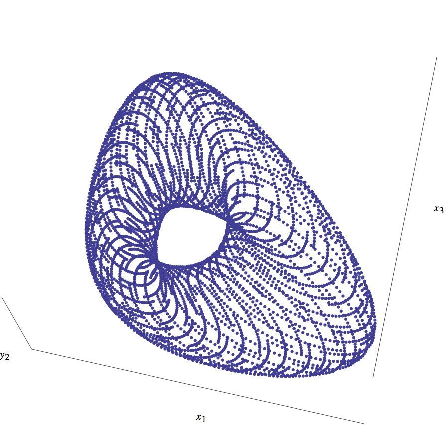
Figure 1: Projection on $\mathbb{R}^{3}$ of an orbit of the map $T_{3}$ (for $\alpha=3$, $\beta=1$)

In addition, $T_{3}$ preserves the 6-volume form

$$\Omega_{3}=(\frac{1}{x_{1}^{2}x_{2}^{2}x_{3}^{2}}-\frac{1}{y_{1}^{2}y_{2}^{2}y_{3}^{2}})dx_{1}\wedge dx_{2}\wedge dx_{3}\wedge dy_{1}\wedge dy_{2}\wedge dy_{3}.$$

The evolution of $T_{3}$ represents a periodic sequence of collisions of six particles $p_{1},\dots,p_{6}$. Denoting by $p_{i}\leftrightarrow p_{j}$ the collision of the particles $p_{i}$ and $p_{j}$, initially we consider the collisions $p_{1}\leftrightarrow p_{2}$, $p_{3}\leftrightarrow p_{4}$ and $p_{5}\leftrightarrow p_{6}$. Subsequently, the collisions $p_{1}\leftrightarrow p_{4}$, $p_{3}\leftrightarrow p_{6}$, $p_{5}\leftrightarrow p_{2}$ and finally the collisions $p_{1}\leftrightarrow p_{6}$, $p_{3}\leftrightarrow p_{2}$ and $p_{5}\leftrightarrow p_{4}$. We proceed periodically with the same sequence of collisions. Here we have considered that all the odd particles carry the same mass $\alpha$ and the even particles the mass $\beta$.

The case for $n=2$ is simpler. According to proposition 3.1, the transfer map

$$T_{2}(x_{1},x_{2},y_{1},y_{2})=(y_{1}\frac{\alpha x_{1}+\beta y_{1}}{\beta x_{1}+\alpha y_{1}},y_{2}\frac{\alpha x_{2}+\beta y_{2}}{\beta x_{2}+\alpha y_{2}},x_{2}\frac{\alpha x_{2}+\beta y_{2}}{\beta x_{2}+\alpha y_{2}},x_{1}\frac{\alpha x_{1}+\beta y_{1}}{\beta x_{1}+\alpha y_{1}}),$$

has three functionally independent integrals, namely $E_{2}$, $P_{2}$ and $H_{2}$ and preserves the 4-volume form

$$\Omega_{2}=(\frac{1}{x_{1}^{2}x_{2}^{2}}-\frac{1}{y_{1}^{2}y_{2}^{2}})dx_{1}\wedge dx_{2}\wedge dy_{1}\wedge dy_{2},$$

therefore it is superintegrable.

The evolution of $T_{2}$ represents the periodic sequence of collisions of four particles $(p_{1}\leftrightarrow p_{2}$, $p_{3}\leftrightarrow p_{4})$ and $(p_{1}\leftrightarrow p_{4},p_{3}\leftrightarrow p_{2})$.

3.2 Transfer maps as reductions of higher-dimensional integrable maps on an invariant manifold

In a similar way we can treat any transfer map which represent different sequences of collisions and derive integrals from the spectrum of the corresponding monodromy matrix. Nevertheless, in order to claim complete integrability in the Liouville sense any transfer map in question should be symplectic with respect to a suitable symplectic structure and the integrals must be in involution. Even if we haven’t found such symplectic structure, we will show that the transfer maps of the YB map (10) can be derived from the restriction of symplectic maps of twice dimension on an invariant manifold.

We consider the four-dimensional YB map

$$\tilde{R}_{\alpha,\beta}:((x_{1},x_{2}),(y_{1},y_{2}))\mapsto((u_{1},u_{2}),(v_{1},v_{2}))$$

that is derived from the unique solution with respect to $u_{i}$, $v_{i}$ of the Lax equation

$$\tilde{L}(u_{1},u_{2},\alpha,\zeta)\tilde{L}(v_{1},v_{2},\alpha,\zeta)=\tilde{L}(y_{1},y_{2},\beta,\zeta)\tilde{L}(x_{1},x_{2},\alpha,\zeta),$$

where

$$\tilde{L}(x_{1},x_{2},\alpha,\zeta)=\left(\begin{array}[]{cc}\frac{\zeta}{\alpha}+x_{1}&x_{2}\\ \frac{1-x_{1}^{2}}{x_{2}}&\frac{\zeta}{\alpha}-x_{1}\end{array}\right).$$ (15)

The Lax matrix (15) has been constructed by restriction on particular symplectic leaves of the Sklyanin bracket on polynomial matrices [8, 10]. The YB map $\tilde{R}_{\alpha,\beta}$ is a symplectic quadrirational YB map (case $I$ in [10]). The corresponding invariant Poisson structure is given by the Sklyanin bracket [20, 21], which in this case is equivalent to

$$\{x_{1},x_{2}\}=\frac{x_{2}}{\alpha},\ \{y_{1},y_{2}\}=\frac{y_{2}}{\beta},\ \{x_{i},y_{j}\}=0.$$

This Poisson bracket can be extended to $\mathbb{R}^{2n}\times\mathbb{R}^{2n}$ as

$$\sum_{i=1}^{n}(\frac{x_{2i}}{\alpha}\frac{\partial}{\partial x_{2i-1}}\wedge\frac{\partial}{\partial x_{2i}}+\frac{y_{2i}}{\beta}\frac{\partial}{\partial y_{2i-1}}\wedge\frac{\partial}{\partial y_{2i}}).$$ (16)

Since this Poisson structure is obtained from the Sklyanin bracket, we can show that every transfer map $\tilde{T}_{n}$ of $\tilde{R}_{\alpha,\beta}$ will be Poisson with respect to (16) and the integrals that are derived from the trace of the corresponding monodromy matrix will be in involution.

Now, we observe that by setting $x_{1}=y_{1}=0$ at $\tilde{R}_{\alpha,\beta}$, we derive $u_{1}=v_{1}=0$. Particularly, the manifold $\mathcal{M}=\{(0,x,0,y)/x,y\in\mathbb{R}\}$ is invariant under the map $\tilde{R}_{\alpha,\beta}$. In addition, the reduced Lax matrix $\tilde{L}(0,x,\alpha,\zeta)$ is equivalent to the Lax matrix (11). Therefore we conclude that $\tilde{R}_{\alpha,\beta}$ is reduced to the map (10) on the invariant manifold $\mathcal{M}$. Consequently, any transfer map $\tilde{T}_{n}$ of $\tilde{R}_{\alpha,\beta}$ can be reduced to the transfer map $T_{n}$ of the map (10) by setting $x_{2i-1}=y_{2i-1}=0$, for $i=1,\dots,n$.

In this sense, for any $n$, $T_{n}$ can be regarded as a reduction of the integrable map $\tilde{T}_{n}$ on the invariant manifold $\mathcal{M}_{n}=\{\left((0,x_{1}),\dots,(0,x_{n}),(0,y_{1}),\dots,(0,y_{n})\right)/x_{i},y_{i}\in\mathbb{R}_{>0}\}$ and solutions of $\tilde{T}_{n}$ are reduced to solutions of $T_{n}$, and consequently, to solutions of the corresponding transfer map of the collision map (5).

4 Conclusions

We proved that the change of velocities of two particles after elastic relativistic collision satisfy the YB equation. The corresponding map is equivalent to a quadrirational YB map that admits a Lax representation, which consequently implies a Lax representation of the original collision map. The $2n$-dimensional transfer maps, which represent particular sequences of $n$-particle periodic collisions, preserve the spectrum of the monodromy matrix and a volume form. The 4-dimensional transfer map turned out to be superintegrable, while the orbits of the 6-dimensional map lie on a two dimensional torus.

Furthermore, we showed that the collision map can be regarded as a reduction of an integrable $4$-dimensional YB map on an invariant manifold and an equivalent reduction can be considered for any $2n$-dimensional transfer map. In this sense, we can consider the corresponding transfer maps as integrable. However, strictly speaking we have not proved the Liouville integrability of the transfer maps due to the lack of a suitable Poisson structure and this is an issue that we would like to further investigate in the future. In the same framework it will be interesting to study the integrability of the transfer dynamics as defined by Veselov in [24, 25], as well as reflection maps [5] associated with relativistic collisions and fixed boundary initial value problems.

Regarding higher dimensional relativistic collisions, the conservation of relativistic energy and momentum is not enough to describe the resulting velocities and some additional assumptions have to be considered (for example the scattering angle of the particles). In this way, extra parameters will be involved in the resulting map. We aim to study in the future higher-dimensional collision maps and examine whether they satisfy the YB equation.

We conclude by remarking that this perspective of collisions as YB maps provides a remarkable link back to the origins of the YB equation in the field of statistical mechanics.

References

• [1] Adler V E, Bobenko A I and Suris Yu B 2003 Classification of integrable equations on quad-graphs. The consistency approach Comm. Math. Phys. 233 513–543.
• [2] Adler V E, Bobenko A I and Suris Yu B 2004 Geometry of Yang-Baxter maps: pencils of conics and quadrirational mappings Comm. Anal. Geom. 12 967–1007.
• [3] Baxter R 1972 Partition function of the eight-vertex lattice model Ann. Physics 70 193–228.
• [4] Buchstaber V 1998 The Yang-Baxter transformation Russ. Math. Surveys 53:6 1343–1345.
• [5] Caudrelier V and Zhang Q C 2014 Yang–Baxter and reflection maps from vector solitons with a boundary Nonlinearity 27 1081–1103
• [6] Drinfeld V 1992 On some unsolved problems in quantum group theory Lecture Notes in Math. 1510 1–8.
• [7] Konstantinou-Rizos S and Mikhailov A V 2013 Darboux transformations, finite reduction groups and related Yang-Baxter maps J. Phys. A: Math. Theor. 46 425201.
• [8] Kouloukas T E and Papageorgiou V G 2009 Yang–Baxter maps with first-degree-polynomial $2\times 2$ Lax matrices J. Phys. A: Math. Theor. 42 404012.
• [9] Kouloukas T E and Papageorgiou V G 2011 Entwining Yang-Baxter maps and integrable lattices Banach Center Publ. 93 163–175.
• [10] Kouloukas T E and Papageorgiou V G 2011 Poisson Yang-Baxter maps with binomial Lax matrices J. Math. Phys. 52 073502.
• [11] Kouloukas T E and Papageorgiou V G 2012 3D compatible ternary systems and Yang–Baxter maps J. Phys. A: Math. Theor. 45 345204.
• [12] Nijhoff F W, Quispel G R W, Capel H W 1983 Direct linearization of nonlinear difference-difference equations, Phys. Lett. A 97 125–128.
• [13] Papageorgiou V G, Nijhoff F W and Capel H W 1990 Integrable mappings and nonlinear integrable lattice equations, Phys. Lett. A 147 106–114.
• [14] Papageorgiou V G and Tongas A G 2009 Yang-Baxter maps associated to elliptic curves, arXiv:0906.3258v1.
• [15] Papageorgiou V G and Tongas A G 2007 Yang-Baxter maps and multi-field integrable lattice equations J. Phys. A: Math. Theor. 40 12677.
• [16] Papageorgiou V G, Tongas A G and Veselov AP 2006 Yang-Baxter maps and symmetries of integrable equations on quad-graphs J. Math. Phys. 47 083502.
• [17] Papageorgiou V G, Suris Yu B, Tongas A G and Veselov A P 2010 On Quadrirational Yang-Baxter Maps SIGMA 6 033 9pp.
• [18] Quispel G R W, Capel H W, Papageorgiou V G and Nijhoff F W 1991 Integrable mappings derived from soliton equations, Physica A 173 243–266.
• [19] Shibukawa Y 2007 Dynamical Yang-baxter maps with an invariance condition Publ. Res. Inst. Math. Sci. 43, No 4, 1157–1182
• [20] Sklyanin E K 1982 Some algebraic structures connected with the Yang-Baxter equation Funct. Anal. Appl. 16, No 4, 263–270.
• [21] Sklyanin E K 1985 The Goryachev-Chaplygin top and the method of the inverse scattering problem Journal of Soviet Mathematics 31, No 6, 3417–3431.
• [22] Sklyanin E K 1988 Classical limits of SU(2)-invariant solutions of the Yang-Baxter equation J. Soviet Math. 40, No 1, 93–107.
• [23] Suris Y B and Veselov A P 2003 Lax matrices for Yang–Baxter maps J. Nonlin. Math. Phys. 10 223–230.
• [24] Veselov A P 2003 Yang-Baxter maps and integrable dynamics Phys. Lett. A 314 214–221.
• [25] Veselov A P 2007 Yang-Baxter maps: dynamical point of view Combinatorial Aspects of Integrable Systems (Kyoto, 2004) MSJ Mem. 17 145–67.
• [26] Weinstein A, Xu P 1992 Classical solutions to the Quantum Yang-Baxter equation, Commun. Math. Phys. 148 309–343.
• [27] Yang C 1967 Some exact results for the many-body problem in one dimension with repulsive delta-function interaction Phys. Rev. Lett. 19 1312–1315.