Consistency of the plug-in functional predictor of the Ornstein-Uhlenbeck process in Hilbert and Banach spaces

Summary

New results on functional prediction of the Ornstein-Uhlenbeck process in an autoregressive Hilbert-valued and Banach-valued frameworks are derived. Specifically, consistency of the maximum likelihood estimator of the autocorrelation operator, and of the associated plug-in predictor is obtained in both frameworks.

Published in Statistics & Probability Letters 117:12–22. DOI: doi.org/10.1016/j.spl.2016.04.023

Key words: Autoregressive Hilbertian processes; Banach-valued autoregressive processes; consistency; maximum likelihood parameter estimator; Ornstein-Uhlenbeck process.

1 Introduction

This paper derives new results in the context of linear processes in function spaces. An extensive literature has been developed in this context in the last few decades (see, for example, Bosq [2000], Ferraty and Vieu [2006], Ramsay and Silverman [2005]; among others). In particular, the problem of functional prediction of linear processes in Hilbert and Banach spaces has been widely addressed. We refer to the reader to the papers by Bensmain and Mourid [2001], Bosq [1996, 2002, 2004, 2007], Guillas [2000, 2001], Mas [2002, 2004, 2007], Mas and Menneteau [2003a], Menneteau [2005], Labbas and Mourid [2002], Mokhtari and Mourid [2003], Mourid [2002, 2004] Rachedi [2004, 2005], Rachedi and Mourid [2003], Dedecker and Merlevède [2003], Dehling and Sharipov [2005], Glendinning and Fleet [2007], Kargin and Onatski [2008], Ruiz-Medina [2012], Pumo [1998], Marion and Pumo [2004] and Turbillon et al. [2007, 2008]; and the references therein. In the above–mentioned papers, different projection methodologies have been adopted in the derivation of the main asymptotic properties of the formulated functional parameter estimators and predictors. Particularly, Bosq [2000], Bosq and Blanke [2007] apply Functional Principal Component Analysis (FPCA); Antoniadis and Sapatinas [2003], Antoniadis et al. [2006], Laukaitis and Vasilecas [2009] propose wavelet–bases–based estimation methods. Applications of these functional estimation results can be found in the papers by Damon and Guillas [2002], Antoniadis and Sapatinas [2003], Laukaitis [2008], Hörmann and Kokoszka [2011], Ruiz-Medina and Salmerón [2009]; among others.

We here pay attention to the problem of functional prediction of the Ornstein–Uhlenbeck (O.U.) process (see, for example, Uhlenbeck and Ornstein [1930], Wang and Uhlenbeck [1945], for its introduction and properties). See also Doob [1942] for the classical definition of O.U. process from the Langevin (linear) stochastic differential equation. We can find in Kutoyants [2004], Liptser and Shiraev [2001] an explicit expression of the maximum likelihood estimator (MLE) of the scale parameter $\theta,$ characterizing its covariance function. Its strong consistency is proved, for instance, in Kleptsyna and Breton [2002]. We formulate here the O.U. process as an autoregressive Hilbertian process of order one (so–called ARH(1) process), and as an autoregressive Banach–valued process of order one (so–called ARB(1) process). Consistency of the MLE of $\theta$ is applied to prove the consistency of the corresponding MLE of the autocorrelation operator of the O.U. process. We adopt the methodology applied in Bosq [1991], since our interest relies on forecasting the values of the O.U. process over an entire time interval. Specifically, considering the O.U. process $\left\{\xi_{t},\ t\in\mathbb{R}\right\}$ on the basic probability space $(\Omega,\mathcal{A},\mathcal{P}),$ we can define

$$X_{n}(t)=\xi_{nh+t},\quad 0\leq t\leq h,\quad n\in\mathbb{Z},$$ (1)

satisfying

$$X_{n}\left(t\right)=\xi_{nh+t}=\int_{-\infty}^{nh+t}e^{-\theta\left(nh+t-s\right)}dW_{s}=\rho_{\theta}\left(X_{n-1}\right)\left(t\right)+\varepsilon_{n}\left(t\right),\quad n\in\mathbb{Z},$$ (2)

with

$$\rho_{\theta}\left(x\right)\left(t\right) = e^{-\theta t}x\left(h\right),\quad\rho_{\theta}\left(X_{n-1}\right)\left(t\right)=e^{-\theta t}\int_{-\infty}^{nh}e^{-\theta\left(nh-s\right)}dW_{s},$$

$$\varepsilon_{n}\left(t\right) = \int_{nh}^{nh+t}e^{-\theta\left(nh+t-s\right)}dW_{s},$$

for $0\leq t\leq h$, where $W=\left\{W_{t},\ t\in\mathbb{R}\right\}$ is a standard bilateral Wiener process (see Supplementary Material 5). Thus, $X=\left\{X_{n},\ n\in\mathbb{Z}\right\}$ satisfies the ARH(1) equation (2) (see also equation (4) below for its general definition). The real separable Hilbert space $H$ is given by $H=L^{2}\left(\left[0,h\right],\beta_{\left[0,h\right]},\lambda+\delta_{(h)}\right),$ where $\beta_{\left[0,h\right]}$ is the Borel $\sigma$-algebra generated by the subintervals in $\left[0,h\right],$ $\lambda$ is the Lebesgue measure and $\delta_{(h)}(s)=\delta\left(s-h\right)$ is the Dirac measure at point $h.$ The associated norm

$$\|f\|_{H}=\sqrt{\displaystyle\int_{0}^{h}\left(f(t)\right)^{2}dt+\left(f(h)\right)^{2}},\quad f\in H=L^{2}\left(\left[0,h\right],\beta_{\left[0,h\right]},\lambda+\delta_{(h)}\right),$$

establishes the equivalent classes of functions given by the relationship $f\sim_{\lambda+\delta_{(h)}}g$ if and only if

$$\left(\lambda+\delta_{(h)}\right)\left(\left\{t:f\left(t\right)\neq g\left(t\right)\right\}\right)=0,$$

with

$$\left(\lambda+\delta_{(h)}\right)\left(\left\{t:f\left(t\right)\neq g\left(t\right)\right\}\right)=0\Leftrightarrow\lambda\left(\left\{t:f\left(t\right)\neq g\left(t\right)\right\}\right)=0\text{ and }f\left(h\right)=g\left(h\right),$$

where, as before, $\delta_{(h)}$ is the Dirac measure at point $h$. We will prove, in Lemma 1 below, that $X=\left\{X_{n},\ n\in\mathbb{Z}\right\},$ constructed in (1) from the O.U. process, satisfying equations (2)–(LABEL:A2:40), is the unique stationary solution to equation (2), in the space $H=L^{2}\left(\left[0,h\right],\beta_{\left[0,h\right]},\lambda+\delta_{(h)}\right),$ admitting a MAH($\infty$) representation. Similarly, in Lemma 4 below, we will prove that $X=\left\{X_{n},\ n\in\mathbb{Z}\right\}$, constructed in (1) from the O.U. process, satisfying equations (2)–(LABEL:A2:40), is the unique stationary solution to equation (2), admitting a MAB($\infty$) representation, in the space $B=\mathcal{C}\left(\left[0,h\right]\right),$ the real separable Banach space of continuous functions, whose support is the interval $\left[0,h\right],$ with the supremum norm.

The main results of this paper provide the almost surely convergence to $\rho_{\theta}$ of its MLE $\rho_{\widehat{\theta}}$, in the norm of $\mathcal{L}(H),$ the space of bounded linear operators in the Hilbert space $H$ (respectively, in the norm of $\mathcal{L}(B),$ the space of bounded linear operators in the Banach space $B$). The convergence in probability of the associated plug–in ARH(1) and ARB(1) predictors (i.e., the convergence in probability of $\rho_{\widehat{\theta}}(X_{n-1})$ to $\rho_{\theta}(X_{n-1})$ in $H$ and $B,$ respectively) is proved as well.

The outline of this paper is as follows. In Appendix 2, the main results of this paper are obtained. Specifically, Appendix 2.1 provides the definition of an O.U. process as an ARH(1) process. Strong consistency in $\mathcal{L}(H)$ of the estimator of the autocorrelation operator is derived in Appendix 2.2. Consistency in $H$ of the associated plug–in ARH(1) predictor is then established in Appendix 2.3. The corresponding results in Banach spaces are given in Appendix 2.4. For illustration purposes, a simulation study is undertaken in Appendix 3. Final comments can be found in Appendix 4. The basic preliminary elements, applied in the proof of the main results of this paper, and the proof of Lemma 1, can be found in the Supplementary Material 5.

2 Prediction of O.U. processes in Hilbert and Banach spaces

In this section, we consider $H$ to be a real separable Hilbert space. Recall that a zero–mean ARH(1) process $X=\left\{X_{n},\ n\in\mathbb{Z}\right\}$, on the basic probability space $(\Omega,\mathcal{A},\mathcal{P}),$ satisfies (see Bosq [2000])

$$X_{n}(t)=\rho\left(X_{n-1}\right)(t)+\varepsilon_{n}(t),\quad n\in\mathbb{Z},\quad\rho\in\mathcal{L}(H),$$ (4)

where $\rho$ denotes the autocorrelation operator of process $X.$ Here, $\varepsilon=\left\{\varepsilon_{n},\ n\in\mathbb{Z}\right\}$ is assumed to be a strong–white noise; i.e., $\varepsilon$ is a Hilbert–valued zero-mean stationary process, with independent and identically distributed components in time, with $\sigma^{2}={\rm E}\left\{\|\varepsilon_{n}\|_{H}^{2}\right\}<\infty,$ for all $n\in\mathbb{Z}.$

O.U. processes as ARH(1) processes

As commented in Appendix 1, equations (1)–(LABEL:A2:40) provide the definition of an O.U. process as an ARH(1) process, with $H=L^{2}\left(\left[0,h\right],\beta_{\left[0,h\right]},\lambda+\delta_{(h)}\right).$ The norm in the space $H$ of $\rho_{\theta}(x),$ with $\rho_{\theta}$ introduced in (LABEL:A2:40) and $x\in H,$ is given by

$$\|\rho_{\theta}(x)\|_{H}^{2}=\displaystyle\int_{0}^{h}\left(\rho_{\theta}\left(x\right)\left(t\right)\right)^{2}d\left(\lambda+\delta_{(h)}\right)\left(t\right)=\displaystyle\int_{0}^{h}\left(\rho_{\theta}\left(x\right)\left(t\right)\right)^{2}dt+\left(\rho_{\theta}\left(x\right)\left(h\right)\right)^{2},$$

for each $h>0$. The following lemma provides, for each $k\geq 1,$ the exact value of the norm of $\rho^{k}_{\theta},$ in the space of bounded linear operators on $H.$ As a direct consequence, the existence of an integer $k_{0}$ such that $\|\rho_{\theta}^{k}\|_{\mathcal{L}\left(H\right)}<1,$ for $k\geq k_{0},$ is also derived for $\theta>0.$

Lemma 1

Let us consider $\theta>0$ and $X=\left\{X_{n},\ n\in\mathbb{Z}\right\}$ satisfying equations (1)–(LABEL:A2:40). For each $k\geq 1,$ the uniform norm of $\rho_{\theta}^{k}$ is given by

$$\|\rho_{\theta}^{k}\|_{\mathcal{L}\left(H\right)}=\sqrt{e^{-2\theta(k-1)h}\left(\frac{1+e^{-2\theta h}\left(2\theta-1\right)}{2\theta}\right)}=e^{-\theta(k-1)h}\|\rho_{\theta}\|_{\mathcal{L}\left(H\right)}.$$ (5)

Furthermore, for $k\geq k_{0}=\left[\frac{1}{\theta}+1\right]^{+},$

$$\|\rho_{\theta}^{k}\|_{\mathcal{L}\left(H\right)}<1,$$ (6)

where $[t]^{+}$ denotes the closest upper integer of $t,$ for every $t\in\mathbb{R}_{+}.$

The proof of this lemma can be found in the Supplementary Material 5 provided.

Remark 1

From equation (6), applying [Bosq, 2000, Theorem 3.1], Lemma 1 implies that $X$ constructed in (1) from an O.U. process, defines the unique stationary solution to equation (2) in the space $H=L^{2}\left(\left[0,h\right],\beta_{\left[0,h\right]},\lambda+\delta_{(h)}\right),$ admitting the MAH($\infty$) representation

$$X_{n}=\displaystyle\sum_{k=0}^{+\infty}\rho_{\theta}^{k}\left(\varepsilon_{n-k}\right),\quad n\in\mathbb{Z},\quad\rho_{\theta}\in\mathcal{L}\left(H\right).$$

Remark 2

Note that, for all $x\in H,$ and $k\geq 2,$ $\|\rho_{\theta}^{k}\|_{\mathcal{L}\left(H\right)}\leq\|\rho_{\theta}\|_{\mathcal{L}\left(H\right)}^{k}.$

Functional parameter estimation and consistency

We now prove the strong consistency of the estimator $\rho_{\widehat{\theta}_{n}}$ of operator $\rho_{\theta}$ in $\mathcal{L}(H),$ with, as before, $H=L^{2}\left(\left[0,h\right],\beta_{\left[0,h\right]},\lambda+\delta_{(h)}\right),$ and $\widehat{\theta}_{n}$ denoting the MLE of $\theta,$ based on the observation of an O.U. process on the interval $[0,T],$ with $T=nh.$ Note that, from equation (LABEL:A2:40), for all $x\in H,$ and for a given sample size $n,$

$$\rho_{\widehat{\theta}_{n}}(x)=e^{-\widehat{\theta}_{n}t}x\left(h\right),$$

where the MLE of $\theta$ is given, for $T=nh,$ by

$$\widehat{\theta}_{T} = \frac{1+\frac{\xi_{0}^{2}}{T}-\frac{\xi_{T}^{2}}{T}}{\frac{2}{T}\displaystyle\int_{0}^{T}\xi_{t}^{2}dt},\quad T>0,$$ (7)

with $\left\{\xi_{t},\ t\in[0,T]\right\}$ being the observed values of the O.U. process over the interval $[0,T].$ Thus, $\rho_{\widehat{\theta}_{n}}$ is introduced in an abstract way, since it can only be explicitly computed, for each particular function $x\in H$ considered. However, the norm $\|\rho_{\theta}-\rho_{\widehat{\theta}_{n}}\|_{\mathcal{L}\left(H\right)}$ is explicitly computed in equation (8) below.

The following results will be applied in the proof of Proposition 1.

Lemma 2

If $t\in\left[0,+\infty\right)$, it holds that

$$|e^{-ut}-e^{-vt}|\leq|u-v|t,\quad u,v\geq 0.$$

The proof of this lemma is given in the Supplementary Material 5.

Theorem 1

(See also [Kleptsyna and Breton, 2002, Proposition 2.2] and [Kutoyants, 2004, p. 63 and p. 117]). The MLE of $\theta$ defined in equation (7) is strongly consistent; i.e.,

$$\widehat{\theta}_{T}\longrightarrow\theta\quad a.s.,\quad T\rightarrow\infty.$$

The proof follows from the Ibragimov–Khasminskii’s Theorem.

Proposition 1

Let $H$ be the space $L^{2}\left(\left[0,h\right],\beta_{\left[0,h\right]},\lambda+\delta_{(h)}\right).$ Then, the estimator $\rho_{\widehat{\theta}_{n}}$ of operator $\rho_{\theta},$ based on the MLE $\widehat{\theta}_{n}$ of $\theta$, is strongly consistent in the norm of $\mathcal{L}\left(H\right)$; i.e.,

$$\|\rho_{\theta}-\rho_{\widehat{\theta}_{n}}\|_{\mathcal{L}\left(H\right)}\longrightarrow 0\quad a.s.,\quad n\rightarrow\infty.$$

Proof. The following straightforward almost surely identities are obtained:

$$\|\rho_{\theta}-\rho_{\widehat{\theta}_{n}}\|_{\mathcal{L}\left(H\right)} = \displaystyle\sup_{x\in H}\left\{\frac{\|\left(\rho_{\theta}-\rho_{\widehat{\theta}_{n}}\right)\left(x\right)\|_{H}}{\|x\|_{H}}\right\}$$

$$= \displaystyle\sup_{x\in H}\left\{\sqrt{\frac{\displaystyle\int_{0}^{h}\left(\left(\rho_{\theta}-\rho_{\widehat{\theta}_{n}}\right)\left(x\right)\left(t\right)\right)^{2}d\left(\lambda+\delta_{(h)}\right)\left(t\right)}{\displaystyle\int_{0}^{h}\left(x\left(t\right)\right)^{2}d\left(\lambda+\delta_{(h)}\right)\left(t\right)}}\right\}$$

$$= \displaystyle\sup_{x\in H}\left\{\sqrt{\left(x\left(h\right)\right)^{2}\frac{\displaystyle\int_{0}^{h}\left(e^{-\theta t}-e^{-\widehat{\theta}_{n}t}\right)^{2}dt+\left(e^{-\theta h}-e^{-\widehat{\theta}_{n}h}\right)^{2}}{\displaystyle\int_{0}^{h}\left(x\left(t\right)\right)^{2}dt+\left(x\left(h\right)\right)^{2}}}\right\}$$

$$= \sqrt{\displaystyle\int_{0}^{h}\left(e^{-\theta t}-e^{-\widehat{\theta}_{n}t}\right)^{2}dt+\left(e^{-\theta h}-e^{-\widehat{\theta}_{n}h}\right)^{2}},$$ (8)

where the last identity is obtained in a similar way to equation (5) in Lemma 1 (see Supplementary Material 5).

From Lemma 2 and equation (8), for $n$ sufficiently large, we have

$$\|\rho_{\theta}-\rho_{\widehat{\theta}_{n}}\|_{\mathcal{L}\left(H\right)} \leq \sqrt{\displaystyle\int_{0}^{h}t^{2}|\theta-\widehat{\theta}_{n}|^{2}dt+h^{2}|\theta-\widehat{\theta}_{n}|^{2}}=|\theta-\widehat{\theta}_{n}|\sqrt{\displaystyle\int_{0}^{h}t^{2}dt+h^{2}}$$ (9)

$$= |\theta-\widehat{\theta}_{n}|h\sqrt{\frac{h}{3}+1}\quad a.s.$$

The strong–consistency of $\rho_{\widehat{\theta}_{n}}$ in $\mathcal{L}\left(H\right)$ directly follows from Theorem 1 and equation (9).

$\blacksquare$

Remark 3

From [Kleptsyna and Breton, 2002, Proposition 2.3] (see also Theorem 2 below), the MLE $\widehat{\theta}_{T}$ of $\theta$ satisfies

$${\rm E}\left\{\left(\theta-\widehat{\theta}_{T}\right)^{2}\right\}=\mathcal{O}\left(\frac{2\theta}{T}\right),\quad T\rightarrow\infty.$$ (10)

In addition, from equation (9), considering $T=nh,$ $h>0,$

$${\rm E}\left\{\|\rho_{\theta}-\rho_{\widehat{\theta}_{n}}\|^{2}_{\mathcal{L}\left(H\right)}\right\}\leq{\rm E}\left\{|\theta-\widehat{\theta}_{n}|^{2}\right\}h^{2}\left(\frac{h}{3}+1\right).$$ (11)

Equations (10)–(11) lead to

$${\rm E}\left\{\|\rho_{\theta}-\rho_{\widehat{\theta}_{n}}\|^{2}_{\mathcal{L}\left(H\right)}\right\}\leq G(\theta,\widehat{\theta}_{n},h),$$

with

$$G(\theta,\widehat{\theta}_{n},h)=\mathcal{O}\left(\frac{2\theta}{n}\right),\quad n\rightarrow\infty.$$

Therefore, the functional parameter estimator $\rho_{\widehat{\theta}_{n}}$ is $\sqrt{n}$–consistent.

Consistency of the plug–in ARH(1) predictor

Let us consider the plug–in ARH(1) predictor $\widehat{X}_{n},$ constructed from the MLE $\rho_{\widehat{\theta}_{n}}$ of $\rho_{\theta}$ in Proposition 1, given by

$$\widehat{X}_{n}\left(t\right)=\rho_{\widehat{\theta}_{n}}\left(X_{n-1}\right)\left(t\right)=e^{-\widehat{\theta}_{n}t}X_{n-1}\left(h\right),\quad 0\leq t\leq h,\quad n\in\mathbb{Z}.$$ (12)

Corollary 1 below provides the consistency of $\widehat{X}_{n},$ given in equation (12), from Proposition 1 by applying the following lemma and theorem.

Lemma 3

Let $\left\{Z_{n},\ n\in\mathbb{Z}\right\}$ be a sequence of random variables such that

$$Z_{n}\sim\mathcal{N}\left(0,\frac{1}{2\theta}\right),\quad\theta>0,$$

and let $\left\{Y_{n},\ n\in\mathbb{Z}\right\}$ be another sequence of random variables such that

$$\sqrt{\ln\left(n\right)}Y_{n}\longrightarrow^{p}0,\quad n\rightarrow\infty.$$

Then,

$$Y_{n}|Z_{n}|\longrightarrow^{p}0,\quad n\rightarrow\infty,$$

where, as usual, $\longrightarrow^{p}$ indicates convergence in probability.

The proof of this lemma can be found in the Supplementary Material 5.

Theorem 2

Let $\widehat{\theta}_{T}$ be the MLE of $\theta$ defined in equation (7), with $\theta>0.$ Hence,

$${\rm E}\left\{\left(\theta-\widehat{\theta}_{T}\right)^{2}\right\}=\mathcal{O}\left(\frac{2\theta}{T}\right),\quad T\rightarrow\infty.$$ (13)

In particular,

$$\lim_{T\rightarrow\infty}{\rm E}\left\{\left(\theta-\widehat{\theta}_{T}\right)^{2}\right\}=0.$$

The proof of this result is given in [Kleptsyna and Breton, 2002, Proposition 2.3].

Corollary 1

Let $H=L^{2}\left(\left[0,h\right],\beta_{\left[0,h\right]},\lambda+\delta_{(h)}\right)$ be the Hilbert space introduced above. Then, the plug–in ARH(1) predictor (12) of an O.U. process is consistent in $H$; i.e.,

$$\left\|\left(\rho_{\theta}-\rho_{\widehat{\theta}_{n}}\right)\left(X_{n-1}\right)\right\|_{H}\longrightarrow^{p}0.$$

Proof. By definition,

$$\left\|\left(\rho_{\theta}-\rho_{\widehat{\theta}_{n}}\right)\left(X_{n-1}\right)\right\|_{H}=\left|X_{n-1}\left(h\right)\right|\sqrt{\displaystyle\int_{0}^{h}\left(e^{-\theta t}-e^{-\widehat{\theta}_{n}t}\right)^{2}dt+\left(e^{-\theta h}-e^{-\widehat{\theta}_{n}h}\right)^{2}}.$$ (14)

From equations (8)–(9) and (14), we then obtain, for $n$ sufficiently large,

$$\left\|\left(\rho_{\theta}-\rho_{\widehat{\theta}_{n}}\right)\left(X_{n-1}\right)\right\|_{H}\leq\left|X_{n-1}\left(h\right)\right|\left|\theta-\widehat{\theta}_{n}\right|h\sqrt{\frac{h}{3}+1}\quad a.s.$$ (15)

Let us set

$$\left\{Y_{n},\ n\in\mathbb{Z}\right\}=\left\{|\theta-\widehat{\theta}_{n}|h\sqrt{\frac{h}{3}+1},\ n\in\mathbb{Z}\right\},\quad\left\{Z_{n},\ n\in\mathbb{Z}\right\}=\left\{X_{n-1}\left(h\right),\ n\in\mathbb{Z}\right\},$$

with $Z_{n}\sim\mathcal{N}\left(0,\frac{1}{2\theta}\right),$ for every $n\in\mathbb{Z}.$ From Theorem 1,

$$Y_{n}\longrightarrow 0\quad a.s.,\quad n\rightarrow\infty.$$

Hence, to apply Lemma 3, we need to prove that

$$\sqrt{\ln\left(n\right)}Y_{n}\longrightarrow^{p}0,\quad n\rightarrow\infty.$$

From the Chebyshev’s inequality and Theorem 2, we get, for all $\varepsilon>0,$

$$\lim_{n\rightarrow 0}\mathcal{P}\left(|\theta-\widehat{\theta}_{n}|\sqrt{\ln\left(n\right)}h\sqrt{\frac{h}{3}+1}\geq\varepsilon\right)\leq\frac{h^{2}\left(\frac{h}{3}+1\right)\ln\left(n\right){\rm E}\left\{\left|\theta-\widehat{\theta}_{n}\right|^{2}\right\}}{\varepsilon^{2}}=0.$$

Therefore, from Lemma 3, we obtain the convergence in probability of $\left\|\left(\rho_{\theta}-\rho_{\widehat{\theta}_{n}}\right)\left(X_{n-1}\right)\right\|_{H}$ to zero.

$\blacksquare$

Prediction of O.U. processes in $B=\mathcal{C}\left(\left[0,h\right]\right)$

As before, let $B$ be now the Banach space of continuous functions, whose support is the interval $\left[0,h\right]$, with the supremum norm, denoted as $\mathcal{C}\left(\left[0,h\right]\right).$ The following lemma states that $\|\rho_{\theta}^{k}\|_{\mathcal{L}\left(B\right)}\leq 1,$ for $\theta>0,$ and for every $k\geq 1,$ with $\mathcal{L}\left(B\right)$ being the space of bounded linear operators on the Banach space $B=\mathcal{C}\left(\left[0,h\right]\right),$ and $\rho_{\theta}$ being introduced in equation (LABEL:A2:40). Consequently, from [Bosq, 2000, Theorem 6.1], $X=\left\{X_{n},\ n\in\mathbb{Z}\right\},$ constructed in (1) from the O.U. process, defines the unique stationary solution to equation (2), in the Banach space $B=\mathcal{C}\left(\left[0,h\right]\right),$ admitting a MAB($\infty$) representation.

Lemma 4

Let $\rho_{\theta}$ introduced in (LABEL:A2:40), defined on $B=\mathcal{C}\left(\left[0,h\right]\right).$ Then, for $k\geq 1,$ $\|\rho_{\theta}^{k}\|_{\mathcal{L}\left(B\right)}\leq 1,$ with $\theta>0.$

Proof.

From

$$\rho_{\theta}^{k}(x)(t)=e^{-\theta t}e^{-\theta(k-1)h}x(h),$$

for each $k\geq 1$ and $\theta>0,$ we have

$$\left\|\rho_{\theta}^{k}\right\|_{\mathcal{L}\left(B\right)} = \displaystyle\sup_{x\in B}\left\{\frac{\|\rho_{\theta}^{k}\left(x\right)\|_{B}}{\|x\|_{B}}\right\}=\displaystyle\sup_{x\in B}\left\{\frac{\displaystyle\sup_{0\leq t\leq h}\left\{\left|e^{-\theta t}e^{-\theta(k-1)h}x(h)\right|\right\}}{\displaystyle\sup_{0\leq t\leq h}\left|x(t)\right|}\right\}$$ (16)

$$= \displaystyle\sup_{x\in B}\left\{\frac{\left|x(h)\right|e^{-\theta(k-1)h}\displaystyle\sup_{0\leq t\leq h}e^{-\theta t}}{\displaystyle\sup_{0\leq t\leq h}\left|x(t)\right|}\right\}\leq\displaystyle\sup_{x\in B}\left\{\frac{\left|x(h)\right|\displaystyle\sup_{0\leq t\leq h}e^{-\theta t}}{\left|x(h)\right|}\right\}$$

$$= \displaystyle\sup_{0\leq t\leq h}e^{-\theta t}=1.$$

$\blacksquare$

We now check the strong consistency of the MLE $\rho_{\widehat{\theta}_{n}}$ of $\rho_{\theta}$ in $\mathcal{L}(B).$ From equation (16),

$$\|\rho_{\theta}-\rho_{\widehat{\theta}_{n}}\|_{\mathcal{L}\left(B\right)}\leq\displaystyle\sup_{0\leq t\leq h}\left\{\left|e^{-\theta t}-e^{-\widehat{\theta}_{n}t}\right|\right\}\quad a.s.$$

From Lemma 2, for $n$ sufficiently large, we then have

$$\|\rho_{\theta}-\rho_{\widehat{\theta}_{n}}\|_{\mathcal{L}\left(B\right)}\leq h\left|\theta-\widehat{\theta}_{n}\right|\quad a.s.$$ (17)

Theorem 1 then leads to the desired result on strong consistency of the estimator $\rho_{\widehat{\theta}_{n}}$ of $\rho_{\theta}$ in $\mathcal{L}(B).$ Furthermore, from Theorem 2 , in a similar way to Remark 3, the $\sqrt{n}$–consistency of $\rho_{\widehat{\theta}_{n}}$ in $\mathcal{L}\left(B\right)$ also follows from equations (13) and (17).

Similarly to Corollary 1, in the following result, the consistency, in the Banach space $B=C([0,h]),$ of the plug–in predictor (12) is obtained.

Corollary 2

The ARB(1) plug–in predictor (12) of a zero–mean O.U. process is consistent in $B=C([0,h])$; i.e., as $n\rightarrow\infty,$

$$\left\|\left(\rho_{\theta}-\rho_{\widehat{\theta}_{n}}\right)\left(X_{n-1}\right)\right\|_{B}\longrightarrow^{p}0.$$

Proof. From Lemma 2, for $n$ sufficiently large, and for each $h>0,$

$$\|\left(\rho_{\theta}-\rho_{\widehat{\theta}_{n}}\right)\left(X_{n-1}\right)\|_{B}=\displaystyle\sup_{0\leq t\leq h}\left\{\left|e^{-\theta t}-e^{-\widehat{\theta}_{n}t}\right|\left|X_{n-1}\left(h\right)\right|\right\}\leq h|\theta-\widehat{\theta}_{n}||X_{n-1}\left(h\right)|\quad a.s.$$ (18)

As derived in the proof of Corollary 1, from Theorem 2, the random sequence $\left\{Y_{n},\ n\in\mathbb{Z}\right\}=\left\{h|\theta-\widehat{\theta}_{n}|,\ n\in\mathbb{Z}\right\}$ is such that

$$\sqrt{\ln\left(n\right)}Y_{n}\leq\sqrt{\frac{h}{3}+1}\sqrt{\ln\left(n\right)}Y_{n}\longrightarrow^{p}0,\quad n\rightarrow\infty.$$

Moreover, $\left\{Z_{n},\ n\in\mathbb{Z}\right\}=\left\{X_{n-1}\left(h\right),\ n\in\mathbb{Z}\right\}$ is such that $Z_{n}\sim\mathcal{N}\left(0,\frac{1}{2\theta}\right).$ Lemma 3 then leads, as $n\rightarrow\infty,$ to the desired convergence result from equation (18):

$$\|\left(\rho_{\theta}-\rho_{\widehat{\theta}_{n}}\right)\left(X_{n-1}\right)\|_{B}\leq Y_{n}|Z_{n}|\longrightarrow^{p}0.$$

$\blacksquare$

3 Simulations

In this section, a simulation study is undertaken to illustrate the asymptotic results presented in this paper about the MLE $\widehat{\theta}_{n}$ of $\theta,$ and the consistency of the ML functional parameter estimators of the autocorrelation operator, and the associated plug–in predictors, in the ARH(1) and ARB(1) frameworks.

Estimation of the scale parameter $\theta$

On the simulation of the sample–paths of an O.U. process, an extension of the Euler’s method, the so–called Euler–Murayama’s method (see Kloeden and Platen [1992]) is applied, from the Langevin stochastic differential equation satisfied by the O.U. process $\left\{\xi_{t},\ t\in\left[0,T\right]\right\}$

$$d\xi_{t}=-\theta\xi_{t}+dW_{t},\quad\theta>0,\quad t\in\left[0,T\right],\quad\xi_{0}=x_{0}.$$ (19)

Thus, let $0=t_{0}<t_{1}<\dots<t_{n}=T$ be a partition of the real interval $\left[0,T\right].$ Then, (19) can be discretized as

$$\widehat{\xi}_{i+1}=\widehat{\xi}_{i}-\theta\widehat{\xi}_{i}+\Delta W_{i},\quad\widehat{\xi}_{0}=\xi_{0}=0,$$ (20)

where $\left\{\Delta W_{i},\ i=0,\dots,n-1\right\}$ are i.i.d. Wiener increments; i.e.,

$$\Delta W_{i}\sim\mathcal{N}\left(0,\Delta t\right)=\sqrt{\Delta t}\mathcal{N}\left(0,1\right),\quad i=0,\dots,n-1.$$

In the following, we take $\Delta t=0.02$ as discretization step size, considering $N=1000$ simulations of the O.U. process. In particular, Figure 1 shows some realizations of the discrete version of the solution to (19) generated from (20).

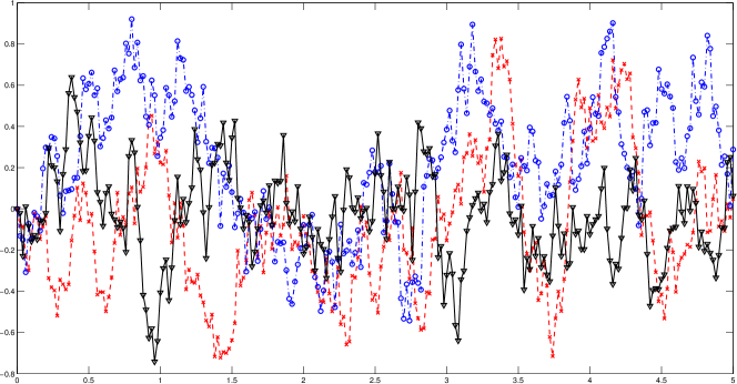
Figure 1: Sample paths of an O.U. process $\left\{\xi_{t},\ 0\leq t\leq T\right\}$ generated with $T=5$, $\Delta t=0.02$, $\theta=5$ and $\widehat{\xi}_{0}=0$.

Let us first illustrate the asymptotic normal distribution of $\widehat{\theta}_{T}$; i.e., for $T$ sufficiently large, we can consider $\widehat{\theta}_{T}\sim\mathcal{N}\left(\theta,\frac{2\theta}{T}\right)$ (see Theorem 3 in the Supplementary Material 5). From equation (7), we take

$$\widehat{\theta}_{T}=\frac{-\displaystyle\int_{0}^{T}\xi_{t}d\xi_{t}}{\displaystyle\int_{0}^{T}\xi_{t}^{2}dt},$$

(see also Supplementary material 5), to compute the following approximation of the MLE $\widehat{\theta}_{T}$ of $\theta,$ for each one of the $N=1000$ simulations performed, and for each one of the six values of parameter $\theta$ considered:

$$\widehat{\theta}_{T}\simeq\frac{-\displaystyle\sum_{i=0}^{n-1}\widehat{\xi}_{t_{i},s}(\theta)\left(\widehat{\xi}_{t_{i+1},s}(\theta)-\widehat{\xi}_{t_{i},s}(\theta)\right)}{\displaystyle\sum_{i=0}^{n-1}\widehat{\xi}_{t_{i},s}^{2}(\theta)\Delta t},\quad t_{0}=0,\leavevmode\nobreak\ t_{n}=T,\leavevmode\nobreak\ \Delta t=0.02,\ \leavevmode\nobreak\ s=1,\dots,N,$$ (21)

where $\widehat{\xi}_{t_{i},s}(\theta)$ represents the $s$–th discrete generation of the O.U. process, evaluated at time $t_{i},$ with covariance scale parameter $\theta,$ for

$$\theta=\left[0.1,0.4,0.7,1,2,5\right].$$

Table 1 displays the empirical probabilities of the error $\widehat{\theta}_{T}-\theta$ to be within the band $\pm 3\sqrt{\frac{2\theta}{T}},$ from $N=1000$ discrete simulations of the O.U. process, considering different sample sizes $\left\{T_{l}=12000+1000(l-1),\ l=1,\dots,7\right\}$. Figure 2 displays the cases $\theta=0.1$ (at the top) and $\theta=5$ (at the bottom). It can be observed that, for each one of the sample sizes considered, $\left\{T_{l}=12000+1000(l-1),\ l=1,\dots,7\right\}$, approximately a 99% of the realizations of $\widehat{\theta}_{T}-\theta$ lie within the band $\pm 3\sqrt{\frac{2\theta}{T}},$ which supports the asymptotic Gaussian distribution.

Table 1: Empirical probabilities of the error of the MLE of $\theta$ to lie within the band $\pm 3\sigma=\pm 3\sqrt{\frac{2\theta}{T}},$ for different sample sizes $T,$ and values of parameter $\theta$.

	Parameter $\theta$
$T$	$0.1$	$0.4$	$0.7$	$1$	$2$	$5$
$12000$	$0.998$	$1$	$0.998$	$0.998$	$1$	$0.998$
$13000$	$0.997$	$0.998$	$0.998$	$1$	$0.995$	$1$
$14000$	$0.998$	$0.997$	$1$	$0.997$	$1$	$0.998$
$15000$	$0.998$	$0.997$	$0.998$	$0.998$	$1$	$0.998$
$16000$	$0.997$	$0.995$	$0.997$	$0.998$	$1$	$1$
$17000$	$0.993$	$0.998$	$1$	$0.997$	$0.995$	$1$
$18000$	$0.997$	$0.997$	$0.995$	$1$	$1$	$0.998$

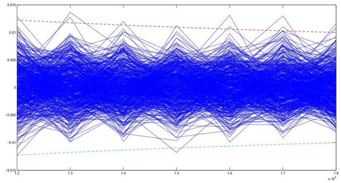
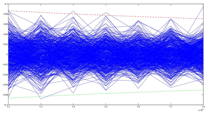
Figure 2: The values of $\widehat{\theta}_{T}-\theta,$ based on $N=1000$ simulations of the O.U. process over the interval $[0,T],$ for $\left\{T_{l}=12000+(l-1)1000,\ l=1,\dots,7\right\},$ are represented against the confidence bands given by $+3\sigma=3\sqrt{\frac{2\theta}{T}}$ (upper red dotted line) and $-3\sigma=-3\sqrt{\frac{2\theta}{T}}$ (lower green dotted line), for values $\theta=0.1$ (at the top) and $\theta=5$ (at the bottom).

Regarding asymptotic efficiency stated in Theorem 2, from $N=1000$ simulations of the O.U. process over the interval $[0,T],$ for $\left\{T_{l}=50+250(l-1),\ l=1,\dots,25\right\},$ the corresponding empirical mean square errors

$${\rm EMSE}(N,T,\theta)=\frac{1}{N}\displaystyle\sum_{s=1}^{N}\left(\theta-\widehat{\theta}_{T}(\omega_{s})\right)^{2},\quad N=1000,\quad\theta=\left[0.1,0.4,0.7,1\right],$$

are displayed in Figure 3. Here, $\widehat{\theta}_{T}(\omega_{s})$, with $\omega_{s}\in\Omega,$ $s=1,\dots,N,$ represent the respective approximated values (21) of the MLE of $\theta,$ computed from $\xi_{t_{i},s},$ $s=1,\dots,N,$ $t_{i}\in[0,T],$ $i=1,\dots,n.$ It can be observed, from the results displayed in Figure 3, that Theorem 2 holds for $T$ sufficiently large.

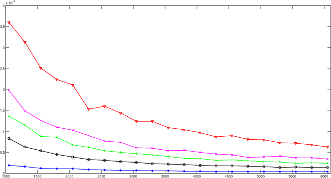
Figure 3: ${\rm EMSE}(N,T,\theta)$ based on $N=1000$ generations of O.U. process, for different sample sizes and values $\theta=0.1$ (blue star line), $\theta=0.4$ (black circles line), $\theta=0.7$ (green plus line), $\theta=1$ (magenta cross line) and $\theta=2$ (red triangle line).

Consistency of $\rho_{\widehat{\theta}_{T}}=\rho_{\widehat{\theta}_{n}}$ in $\mathcal{L}(H)$ and $\mathcal{L}(B)$

The strong–consistency of $\rho_{\widehat{\theta}_{n}}$ in $\mathcal{L}(H)$ is derived in Proposition 1 from the following almost surely upper bound

$$\|\rho_{\theta}-\rho_{\widehat{\theta}_{n}}\|_{\mathcal{L}\left(H\right)}\leq|\theta-\widehat{\theta}_{n}|h\sqrt{\frac{h}{3}+1}\quad a.s.$$ (22)

Here, from $N=1000$ simulations of the O.U. process on the interval $[0,T],$ with sample sizes $T=nh=n=\left\{200000+(l-1)200000,\ l=1,\dots,5\right\},$ the corresponding values of $\widehat{\theta}_{T}-\theta=\widehat{\theta}_{n}-\theta$ are computed, considering the cases $\theta=\left[0.4,0.7,1\right].$ Table 2 shows the empirical probability of $\widehat{\theta}_{T}-\theta$ to lie within the band $\pm 3\sqrt{\frac{2\theta}{T}},$ for each one of sample sizes and cases $\theta=\left[0.4,0.7,1\right]$ regarded. It can be observed that for the sample sizes studied, in the case of $\theta=1,$ the empirical probabilities are equal to one. Thus, the almost surely convergence to zero of the upper bound (22) holds, with an approximated convergence rate of $\sqrt{T}=\sqrt{n}.$ Note that, for the other two cases, $\theta=0.4$ and $\theta=0.7,$ the empirical probabilities are also very close to one (see also Table 1 for smaller sample sizes, where we can also observe the empirical probabilities very close to one for the same band). In particular, Figure 4 displays the cases $\theta=0.4$ (at the top) and $\theta=1$ (at the bottom).

Table 2: Empirical probability of $\widehat{\theta}_{T}-\theta$ to be within the band $\pm 3\sigma=\pm 3\sqrt{\frac{2\theta}{T}},$ from $N=1000$ simulations of an O.U. process over the interval $[0,T],$ with $\left\{T_{l}=200000+(l-1)200000,\ l=1,\dots,5\right\},$ considering the cases $\theta=\left[0.4,0.7,1\right]$.

	Parameter $\theta$
$T$	$0.4$	$0.7$	$1$
$200000$	$1$	$1$	$1$
$400000$	$1$	$1$	$1$
$600000$	$0.999$	$1$	$1$
$800000$	$0.999$	$0.999$	$1$
$1000000$	$0.998$	$1$	$1$

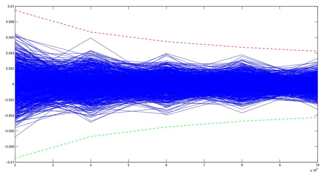
Figure 4: The values of $\widehat{\theta}_{T}-\theta$ are represented, corresponding to $N=1000$ simulations of an O.U. process over the interval $[0,T],$ with $\left\{T_{l}=200000+(l-1)200000,\ l=1,\dots,5\right\},$ considering the cases $\theta=0.4$ (at the top), and $\theta=1$ (at the bottom). The upper red dotted line is $+3\sqrt{\frac{2\theta}{T}}$ and the lower green dotted line is $-3\sqrt{\frac{2\theta}{T}}$.

It can be observed from Table 2 that a better performance is obtained for the largest values of $\theta,$ which corresponds to the weakest dependent case. Furthermore, from the upper bound in (17), the strong consistency of $\rho_{\widehat{\theta}_{n}}$ in $\mathcal{L}(B),$ with, as before, $B=\mathcal{C}([0,h]),$ is also illustrated from the results displayed in Table 2 and Figure 4.

Consistency of the ARH(1) and ARB(1) plug–in predictors for the O.U. process

Let us now consider the derived upper bounds in (15) and (18) in Corollaries 1–2, for the ARH(1) and ARB(1) predictors, respectively. From the generation of $N=1000$ discrete realizations of an O.U. process over the interval $[0,T],$ for $\left\{T_{l}=200000+(l-1)200000,\ l=1,\dots,5\right\},$ the upper bounds (15) and (18) are evaluated, for the cases $\theta=\left[0.4,0.7,1\right].$ The following empirical probabilities for $\epsilon=0.008,$ are reflected in Table 3

$$\widehat{\mathcal{P}}^{H}(N,T,\theta) = 1-\widehat{\mathcal{P}}\left(|X_{n-1}\left(h\right)||\theta-\widehat{\theta}_{n}|h\sqrt{\frac{h}{3}+1}>\epsilon\right),$$ (23)

$$\widehat{\mathcal{P}}^{B}(N,T,\theta) = 1-\widehat{\mathcal{P}}\left(|X_{n-1}\left(h\right)||\theta-\widehat{\theta}_{n}|h>\epsilon\right),$$ (24)

with $N=1000$, $\left\{T_{l}=200000+(l-1)200000,\ l=1,\dots,5\right\}$ and $\theta=\left[0.4,0.7,1\right]$, for the Hilbert–valued and Banach–valued (see (15) and (18)) frameworks (see also Figure 5). It can be observed that the empirical probabilities are equal to one in both frameworks for the largest sample sizes, in any of the cases considered.

Table 3: Empirical probabilities (23)–(24), based on $N=1000$ simulations of the O.U. process over the interval $[0,T],$ for $\left\{T_{l}=200000+(l-1)200000,\ l=1,\dots,5\right\},$ considering the cases $\theta=\left[0.4,0.7,1\right],$ and $\epsilon=0.008$.

	Parameter $\theta$
		Hilbert-valued case			Banach-valued case
$T$	$0.4$	$0.7$	$1$	$0.4$	$0.7$	$1$
$200000$	$0.980$	$0.980$	$0.980$	$0.987$	$0.991$	$0.987$
$400000$	$0.995$	$0.995$	$0.995$	$0.997$	$0.998$	$0.9977$
$600000$	$0.999$	$0.998$	$0.999$	$0.999$	$0.999$	$1$
$800000$	$1$	$0.999$	$0.999$	$1$	$1$	$1$
$1000000$	$1$	$1$	$1$	$1$	$1$	$1$

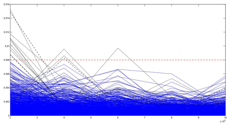
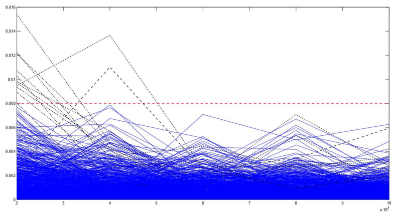
Figure 5: The values of $|X_{n-1}\left(h\right)||\theta-\widehat{\theta}_{n}|h\sqrt{\frac{h}{3}+1}$ (first and second figure) and $|X_{n-1}\left(h\right)||\theta-\widehat{\theta}_{n}|h$ (third and fourth figure) are represented, based on $N=1000$ generations of O.U. process over the interval $[0,T],$ for $\left\{T_{l}=200000+(l-1)200000,\ l=1,\dots,5\right\},$ against $\epsilon=0.008$ (red dotted line), considering $\theta=0.4$ (first and third figure) and $\theta=1$ (second and fourth figure).

The strong–consistency of the MLE of $\theta$ and of the autocorrelation operator of the O.U. process, in Banach and Hilbert spaces, has been first illustrated. The almost surely rate of convergence to zero is shown as well. The numerical results on the consistency of the associated ARH(1) and ARB(1) plug–in predictors then follow, from the computation of the corresponding empirical probabilities for the derived upper bounds. Note that the numerical results displayed in Appendix 3 are obtained under generation of sample sizes ranging from $12000$ up to a million of time instants, considering $1000$ repetitions for each one of such sample sizes. In all these simulations performed, the discretization step size considered has been $\Delta t=0.02.$

4 Final comments

The problem of functional prediction of the O.U. process could be of interest in several applied fields. For example, in finance, in the context of the Vasicek’s model (see Vasicek [1977]) the results derived allow to predict the curve representing the interest rate over a temporal interval, in a consistent way. Note that, in this context, the MLE computed for parameter $\theta$ provides a consistent approximation of the speed reversion, which definitely determines the proposed functional predictor of the interest rate.

Summarizing, this paper addresses the problem of functional prediction of the O.U. process from ARH(1) and ARB(1) perspectives. Specifically, considering the O.U. process as an ARH(1) and an ARB(1) process, new results on strong consistency (almost surely convergence to the true parameter value), in the spaces $\mathcal{L}(H)$ and $\mathcal{L}(B)$ of the MLE of its autocorrelation operator are derived. Consistency results (convergence in probability to the true value) of the associated plug–in predictors are obtained as well. The numerical results shown, in addition, the normality and the asymptotic efficiency of the MLE of the scale parameter $\theta$ of the covariance function of the O.U. process.

5 Supplementary Material

The definition and properties of an O.U. process are given here, as well as the proof of Lemma 1.

Ornstein–Uhlenbeck process

Let $\xi\left(\omega\right)=\left\{\xi_{t}\left(\omega\right),\ t\in\mathbb{R}\right\},$ $\omega\in\Omega,$ be a real–valued sample–path continuous stochastic process defined on the basic probability space $\left(\Omega,\mathcal{A},\mathcal{P}\right),$ with index set the real line $\mathbb{R}.$ As demonstrated in Doob [1942], process $\xi$ is an O.U. process if it provides the Gaussian solution to the following stochastic linear Langevin differential equation:

$$d\xi_{t}=\theta\left(\mu-\xi_{t}\right)dt+\sigma dW_{t},\quad\theta,\leavevmode\nobreak\ \sigma>0,\quad t\in\mathbb{R},$$ (25)

where $W=\left\{W_{t},\ t\in\mathbb{R}\right\}$ is a standard bilateral Wiener process; i.e.,

$$W_{t}=W_{t}^{(1)}\boldsymbol{1}_{\mathbb{R}^{+}}\left(t\right)+W_{-t}^{(2)}\boldsymbol{1}_{\mathbb{R}^{-}}\left(t\right),$$

with $W_{t}^{(1)}$ and $W_{-t}^{(2)}$ being independent standard Wiener processes, and $\boldsymbol{1}_{\mathbb{R}^{+}}$ and $\boldsymbol{1}_{\mathbb{R}^{-}}$ respectively denoting the indicator functions over the positive and negative real line. Applying, in equation (25), the method of separation of variables, considering $f\left(\xi_{t},t\right)=\xi_{t}e^{\theta t},$ we obtain

$$\xi_{t} = \mu+\displaystyle\int_{-\infty}^{t}\sigma e^{-\theta\left(t-s\right)}dW_{s},\quad\theta,\quad\sigma>0,\quad t\in\mathbb{R},$$ (26)

where the integral is understood in the Itô sense (see Ash and Gardner [1975], Sobczyk [1991] for more details). Particularizing to $\xi=\left\{\xi_{t},\ t\in\mathbb{R}^{+}\right\}$, the O.U. process is transformed into

$$\xi_{t}=\xi_{0}e^{-\theta t}+\mu\left(1-e^{-\theta t}\right)+\displaystyle\int_{0}^{t}\sigma e^{-\theta\left(t-s\right)}dW_{s},\quad\theta,\sigma>0,\quad t\in\mathbb{R}^{+}.$$ (27)

It is well–known that the solution $\xi=\left\{\xi_{t},\ t\in\mathbb{R}\right\}$ to the stochastic differential equation

$$d\xi_{t}=\mu\left(\xi_{t},t\right)dt+\sqrt{D\left(\xi_{t},t\right)}dW_{t},\quad t\in\mathbb{R},$$

has marginal probability density function $f\left(x,t\right),$ satisfying the following Fokker–Planck’s scalar equation (see, for example, Kadanoff [2000]):

$$\frac{\partial}{\partial t}f\left(x,t\right)=\frac{-\partial}{\partial x}\left[\mu\left(x,t\right)f\left(x,t\right)\right]+\frac{1}{2}\frac{\partial^{2}}{\partial x^{2}}\left[D\left(x,t\right)f\left(x,t\right)\right],\quad t\in\mathbb{R}.$$

In the case of O.U. process, the stationary solution ($\frac{\partial}{\partial t}f\left(x,t\right)=0$), under $f\left(x,x_{0}\right)=\delta\left(x-x_{0}\right)$, adopts the form

$$f\left(x,t\right)=\sqrt{\frac{\theta}{\pi\sigma^{2}}}e^{\frac{-\theta\left(x-\mu\right)^{2}}{\sigma^{2}}},\quad\theta,\sigma>0,\quad t\in\mathbb{R},$$

which corresponds to the probability density function of a Gaussian distribution with mean $\mu$ and variance $\frac{\sigma^{2}}{2\theta},$ i.e., which corresponds to the probability density function of a random variable $X$ such that

$$X\sim\mathcal{N}\left(\mu,\frac{\sigma^{2}}{2\theta}\right).$$

From (26), the mean and covariance functions of O.U. process (see, for instance, Doob [1942], Uhlenbeck and Ornstein [1930]) can be computed as follows:

$$\mu_{\xi}(t) = {\rm E}\left\{\xi_{t}\right\}=\mu+\sigma{\rm E}\left\{\displaystyle\int_{-\infty}^{t}e^{-\theta\left(t-s\right)}dW_{s}\right\}=\mu,\quad t\in\mathbb{R},$$

$$C_{\xi}(t,s) = {\rm Cov}\left(\xi_{s},\xi_{t}\right)={\rm E}\left\{\left(\xi_{s}-\mu\right)\left(\xi_{t}-\mu\right)\right\}=\sigma^{2}e^{-\theta\left(t+s\right)}{\rm E}\left\{\displaystyle\int_{-\infty}^{t}e^{\theta u}dW_{u}\displaystyle\int_{-\infty}^{s}e^{\theta v}dW_{v}\right\}$$ (28)

$$= \sigma^{2}e^{-\theta\left(t+s\right)}\int_{-\infty}^{\infty}e^{2\theta u}\boldsymbol{1}_{\left[-\infty,t\right]}\left(u\right)\boldsymbol{1}_{\left[-\infty,s\right]}\left(u\right)du=\sigma^{2}e^{-\theta\left(t+s\right)}\int_{-\infty}^{\min\left\{s,t\right\}}e^{2\theta u}du$$

$$= \frac{\sigma^{2}}{2\theta}e^{-\theta\left(t+s\right)}e^{2\theta\min\left\{s,t\right\}}=\frac{\sigma^{2}}{2\theta}e^{-\theta|t-s|},\quad t,s\in\mathbb{R},$$

where ${\rm Cov}\left(X,Y\right)$ denotes the covariance between random variables $X$ and $Y$. Additionally, from (27), we obtain the following identities:

$${\rm E}\left\{\xi_{t}\right\} = \mu e^{-\theta t}+\mu\left(1-e^{-\theta t}\right)=\mu,\quad{\rm E}\left\{\xi_{t}|\xi_{0}=c\right\}=\mu+e^{-\theta t}\left(c-\mu\right),\quad t\in\mathbb{R}^{+},$$

$${\rm Cov}\left(\xi_{s},\xi_{t}|\xi_{0}=c\right) = \frac{\sigma^{2}}{2\theta}e^{-\theta|t-s|}+\left(c^{2}-2c\mu+\mu^{2}\right)e^{-\theta\left(s+t\right)},\quad t,s\in\mathbb{R}^{+},$$

where $c$ is a constant. In the subsequent development, we will consider $\mu=0$ and $\sigma=1$.

Maximum likelihood estimation of the covariance scale parameter $\theta$

The MLE of $\theta$ in (28) is given by (see Graczyk and Jakubowski [2006]; [Kutoyants, 2004, p. 63]; [Liptser and Shiraev, 2001, p. 265])

$$\widehat{\theta}_{T}=\frac{-\displaystyle\int_{0}^{T}\xi_{t}d\xi_{t}}{\displaystyle\int_{0}^{T}\xi_{t}^{2}dt}=\frac{\theta\displaystyle\int_{0}^{T}\xi_{t}^{2}dt-\displaystyle\int_{0}^{T}\xi_{t}dW_{t}}{\displaystyle\int_{0}^{T}\xi_{t}^{2}dt}=\theta-\frac{\displaystyle\int_{0}^{T}\xi_{t}dW_{t}}{\displaystyle\int_{0}^{T}\xi_{t}^{2}dt},\quad\theta,T>0.$$ (29)

Thus, equation (29) becomes

$$\widehat{\theta}_{T} = \frac{1+\frac{\xi_{0}^{2}}{T}-\frac{\xi_{T}^{2}}{T}}{\frac{2}{T}\displaystyle\int_{0}^{T}\xi_{t}^{2}dt},\quad T>0.$$ (30)

We will assume that $T$ is large enough such that $\widehat{\theta}_{T}>0$ almost surely. It is well–known that the MLE $\widehat{\theta}_{T}$ of $\theta$ is strongly consistent (see details in [Kleptsyna and Breton, 2002, Proposition 2.2]; [Kutoyants, 2004, p. 63 and p. 117]).

Theorem 3

The following limit in distribution sense holds for the MLE $\widehat{\theta}_{T}$ of $\theta,$ given in equation (30):

$$\lim_{T\rightarrow\infty}\sqrt{T}\left(\widehat{\theta}_{T}-\theta\right)=\lim_{T\rightarrow\infty}\frac{-\sqrt{T}\displaystyle\int_{0}^{T}\xi_{t}dW_{t}}{\displaystyle\int_{0}^{T}\xi_{t}^{2}dt}=Z,\quad\mbox{with}\quad Z\sim\mathcal{N}\left(0,2\theta\right).$$

Results in [Jiang, 2012, Theorem 1.1 and Corollary 1.1] lead to the following almost surely identities (see also [Bosq, 2000, Theorem 2.10];[Ledoux and Talagrand, 2011, pp. 196–203], in relation to the law of the iterated logarithm)

$$\displaystyle\limsup_{T\to+\infty}\frac{\widehat{\theta}_{T}-\theta}{\sqrt{\frac{4\theta}{T}\displaystyle\ln\left(\displaystyle\ln\left(T\right)\right)}}=1\quad a.s.,$$

$$\displaystyle-\liminf_{T\to+\infty}\frac{\widehat{\theta}_{T}-\theta}{\sqrt{\frac{4\theta}{T}\displaystyle\ln\left(\displaystyle\ln\left(T\right)\right)}}=1\quad a.s.,$$

$$|\theta-\widehat{\theta}_{T}|=\mathcal{O}\left(\sqrt{\frac{4\theta\displaystyle\ln\left(\displaystyle\ln\left(T\right)\right)}{T}}\right)\quad a.s.$$

Preliminary inequalities and results

In this section we recall some inequalities and well–known convergence results on random variables, as well as basic deterministic inequalities, that have been applied in the derivation of the main results displayed above.

Lemma 5

Let $X$ be a zero–mean normal distributed random variable, i.e., $X\sim\mathcal{N}\left(0,\sigma^{2}\right),$ with $\sigma>0$. Then,

$$\mathcal{P}\left(|X|\geq x\right)\leq e^{-\frac{x^{2}}{2\sigma^{2}}},\quad x\geq 0.$$

Proof. Let $X^{\prime}$ be such that $X^{\prime}\sim\mathcal{N}\left(0,1\right).$ Then,

$$\mathcal{P}\left(|X^{\prime}|\geq x\right)=2F_{X^{\prime}}\left(-x\right)=\sqrt{\frac{2}{\pi}}\displaystyle\int_{x}^{\infty}e^{-\frac{t^{2}}{2}}dt,\leavevmode\nobreak\ \forall x\geq 0.$$ (31)

Let us set

$$g\left(x\right) = e^{-\frac{x^{2}}{2}}-\sqrt{\frac{2}{\pi}}\displaystyle\int_{x}^{\infty}e^{-\frac{t^{2}}{2}}dt,\quad g\left(0\right)=0,\quad\lim_{x\rightarrow\infty}g\left(x\right)=0,$$

$$g^{\prime}\left(x\right) = -xe^{-\frac{x^{2}}{2}}+\sqrt{\frac{2}{\pi}}e^{-\frac{x^{2}}{2}}=e^{-\frac{x^{2}}{2}}\left(\sqrt{\frac{2}{\pi}}-x\right).$$

Function $g$ is monotone increasing over $\left(0,\sqrt{\frac{2}{\pi}}\right),$ and $g$ is monotone decreasing over $\left(\sqrt{\frac{2}{\pi}},\infty\right).$

From equations (31)–(LABEL:A2:Supp:32),

$$\mathcal{P}\left(|X^{\prime}|\geq x\right)\leq e^{-\frac{x^{2}}{2}},\quad x\geq 0.$$

Now, consider $X^{\prime}=\frac{X}{\sigma},$ with $X\sim\mathcal{N}\left(0,\sigma^{2}\right),$ then,

$$\mathcal{P}\left(|X|\geq x\right)\leq e^{-\frac{x^{2}}{2\sigma^{2}}},\quad x\geq 0.$$

$\blacksquare$

5.3.1 Proof of Lemma 1

Proof.

Let us first consider the case $k=1,$ from

$$\rho_{\theta}\left(x\right)\left(t\right) = e^{-\theta t}x\left(h\right),\quad\rho_{\theta}\left(X_{n-1}\right)\left(t\right)=e^{-\theta t}\int_{-\infty}^{nh}e^{-\theta\left(nh-s\right)}dW_{s},$$

$$\varepsilon_{n}\left(t\right) = \int_{nh}^{nh+t}e^{-\theta\left(nh+t-s\right)}dW_{s},$$

and

$$\|\rho_{\theta}(x)\|_{H}^{2} = \displaystyle\int_{0}^{h}\left(\rho_{\theta}\left(x\right)\left(t\right)\right)^{2}d\left(\lambda+\delta_{(h)}\right)\left(t\right)=\displaystyle\int_{0}^{h}\left(\rho_{\theta}\left(x\right)\left(t\right)\right)^{2}dt+\left(\rho_{\theta}\left(x\right)\left(h\right)\right)^{2},$$

we have

$$\|\rho_{\theta}\|_{\mathcal{L}\left(H\right)} = \displaystyle\sup_{x\in H}\left\{\frac{\|\rho_{\theta}\left(x\right)\|_{H}}{\|x\|_{H}}\right\}=\sup_{x\in H}\left\{\sqrt{\frac{\left(\displaystyle\int_{0}^{h}e^{-2\theta t}dt+e^{-2\theta h}\right)\left(x\left(h\right)\right)^{2}}{\displaystyle\int_{0}^{h}\left(x\left(t\right)\right)^{2}dt+\left(x\left(h\right)\right)^{2}}}\right\}.$$ (33)

Furthermore,

$$\|\rho_{\theta}\|_{\mathcal{L}\left(H\right)}=\sup_{x\in H}\left\{\sqrt{\frac{\left(\displaystyle\int_{0}^{h}e^{-2\theta t}dt+e^{-2\theta h}\right)\left(x\left(h\right)\right)^{2}}{\displaystyle\int_{0}^{h}\left(x\left(t\right)\right)^{2}dt+\left(x\left(h\right)\right)^{2}}}\right\}\leq\sqrt{\int_{0}^{h}e^{-2\theta t}dt+e^{-2\theta h}}.$$ (34)

Additionally, the function $x_{0}:\leavevmode\nobreak\ [0,h]\longrightarrow\mathbb{R},$ given by

$$x_{0}(t)=\chi_{\mathcal{M}}(t),\quad h\in\mathcal{M}\subset[0,h],\quad\int_{\mathcal{M}}dt=0,$$ (35)

with $\boldsymbol{1}_{\mathcal{M}},$ denoting the indicator function of set $\mathcal{M},$ belongs to $H=L^{2}\left(\left[0,h\right],\beta_{\left[0,h\right]},\lambda+\delta_{(h)}\right),$ since

$$x_{0}^{2}(h)=1,\quad\int_{0}^{h}x_{0}^{2}(t)dt=0\quad\|x_{0}\|_{H}^{2}=\int_{0}^{h}x_{0}^{2}(s)ds+x_{0}^{2}(h)=1.$$

Thus, by definition of $\|\rho_{\theta}\|_{\mathcal{L}(H)},$

$$\frac{\|\rho_{\theta}(x_{0})\|_{H}}{\|x_{0}\|_{H}}=\sqrt{\int_{0}^{h}e^{-2\theta t}dt+e^{-2\theta h}} \leq \|\rho_{\theta}\|_{\mathcal{L}(H)}$$ (36)

Equations (33)–(36) lead to

$$\|\rho_{\theta}\|_{\mathcal{L}\left(H\right)}=\sqrt{\int_{0}^{h}e^{-2\theta t}dt+e^{-2\theta h}}=\sqrt{\frac{1+e^{-2\theta h}\left(2\theta-1\right)}{2\theta}}.$$ (37)

We are now going to compute $\|\rho_{\theta}^{k}\|_{\mathcal{L}\left(H\right)},$ for $k\geq 2.$ Since, for all $x\in H,$

$$\rho_{\theta}^{k}(x)(t)=e^{-\theta t}e^{-\theta(k-1)h}x(h),$$

we obtain

$$\|\rho_{\theta}^{k}\|_{\mathcal{L}\left(H\right)}=\sup_{x\in H}\left\{\sqrt{\frac{\left[e^{-2\theta(k-1)h}\displaystyle\int_{0}^{h}e^{-2\theta t}dt+e^{-2\theta kh}\right]\left(x(h)\right)^{2}}{\displaystyle\int_{0}^{h}\left(x(t)\right)^{2}dt+\left(x(h)\right)^{2}}}\right\}.$$

Considering function $x_{0}$ defined in equation (35), applying similar arguments to those given in the computation of $\|\rho_{\theta}\|_{\mathcal{L}\left(H\right)},$ we have

$$\|\rho_{\theta}^{k}\|_{\mathcal{L}\left(H\right)}=\sqrt{e^{-2\theta(k-1)h}\frac{1+e^{-2\theta h}\left(2\theta-1\right)}{2\theta}}=e^{-\theta(k-1)h}\|\rho_{\theta}\|_{\mathcal{L}\left(H\right)}.$$

Now, from equation (37),

$$\|\rho_{\theta}\|_{\mathcal{L}\left(H\right)}<1\Longleftrightarrow 1-e^{-2\theta h}<2\theta\left(1-e^{-2\theta h}\right)\Longleftrightarrow\theta>\frac{1}{2}.$$

Furthermore, for $\theta\in\left(0,1/2\right]$,

$$\|\rho_{\theta}\|_{\mathcal{L}\left(H\right)}=\sqrt{\alpha\left(\theta\right)}<\sqrt{1+h},$$

since $\sqrt{\alpha\left(\theta\right)}$ is a monotonically decreasing function on $\left(0,1/2\right],$ with $\alpha\left(\theta\right)=1$ if $\theta=\frac{1}{2}$ and $\alpha\left(\theta\right)\to 1+h$, when $\theta\to 0$. Hence, if $\theta(k-1)\geq 1$,

$$\|\rho_{\theta}^{k}\|_{\mathcal{L}\left(H\right)}=e^{-\theta(k-1)h}\sqrt{\alpha\left(\theta\right)}\leq e^{-h}\sqrt{\alpha\left(\theta\right)}<\frac{\sqrt{1+h}}{e^{h}}<1,\quad h>0,$$

which implies that $\|\rho_{\theta}^{k_{0}}\|_{\mathcal{L}\left(H\right)}<1$, when $k_{0}\geq\frac{1}{\theta}+1$.

$\blacksquare$

5.3.2 Proof of Lemma 2

Proof. Let us first assume that $x\geq y>0$.

From the Mean Value Theorem applied over $e^{z}$, there exists $0<\alpha<1$ such that

$$\frac{e^{z+h}-e^{z}}{h}=e^{z+\alpha h}.$$

Taking $z=-xt$ and $z+h=-yt$, we get the following inequalities:

$$|e^{-xt}-e^{-yt}|=|x-y|te^{-xt+\alpha\left(x-y\right)t}=|x-y|te^{xt\left(\alpha-1\right)}e^{-y\alpha t}\leq|x-y|te^{-y\alpha t}\leq|x-y|t.$$

Similar inequalities are obtained for the case $y\geq x>0,$ by applying the Mean Value Theorem over the interval $\left[x,\leavevmode\nobreak\ y\right]$, instead of $\left[y,\leavevmode\nobreak\ x\right]$.

$\blacksquare$

5.3.3 Proof of Lemma 3

Proof. Considering the indicator function $\boldsymbol{1}_{\cdot},$ it holds

$$Y_{n}|Z_{n}| = Y_{n}|Z_{n}|\boldsymbol{1}_{\{|Z_{n}|<a_{n}\}}+Y_{n}|Z_{n}|\boldsymbol{1}_{\{|Z_{n}|\geq a_{n}\}}\leq Y_{n}a_{n}+Y_{n}|Z_{n}|\boldsymbol{1}_{\{|Z_{n}|\geq a_{n}\}},$$ (38)

where $\left\{a_{n},\ n\in\mathbb{Z}\right\}$ is a sequence of positive numbers such that the event $\left\{Y_{n}|Z_{n}|\boldsymbol{1}_{\{|Z_{n}|\geq a_{n}\}},\ n\in\mathbb{Z}\right\}$ is equivalent to $\left\{|Z_{n}|\geq a_{n},\ n\in\mathbb{Z}\right\}$. From (38) and Lemma 5, if we take $a_{n}>\frac{\varepsilon}{2},$ for all $n\in\mathbb{Z},$ we get, for each $\varepsilon>0$,

$$\mathcal{P}\left(Y_{n}|Z_{n}|\geq\varepsilon\right)\leq\mathcal{P}\left(Y_{n}a_{n}\geq\frac{\varepsilon}{2}\right)+\mathcal{P}\left(|Z_{n}|\geq a_{n}\right)\leq\mathcal{P}\left(Y_{n}a_{n}\geq\frac{\varepsilon}{2}\right)+e^{-\theta a_{n}^{2}}.$$ (39)

For $a_{n}=c\sqrt{\ln\left(n\right)}>\frac{\varepsilon}{2}$, with $\frac{1}{\sqrt{\theta}}<c<+\infty$,

$$\sum_{n\in\mathbb{Z}}\mathcal{P}\left(|Z_{n}|\geq a_{n}\right)\leq\displaystyle\sum_{n\in\mathbb{Z}}e^{-\theta a_{n}^{2}}=\displaystyle\sum_{n\in\mathbb{Z}}\frac{1}{n^{\theta c^{2}}}<+\infty,$$

which implies that

$$\lim_{n\rightarrow\infty}\mathcal{P}\left(|Z_{n}|\geq a_{n}\right)=0$$

in equation (39).

On the other hand, since $\sqrt{\ln\left(n\right)}Y_{n}\longrightarrow^{p}0,$ for every $\varepsilon>0,$

$$0=\lim_{n\rightarrow\infty}\mathcal{P}\left(\sqrt{\ln\left(n\right)}Y_{n}\geq\frac{\varepsilon}{2}\right)=\lim_{n\rightarrow\infty}\mathcal{P}\left(Y_{n}\frac{a_{n}}{c}\geq\frac{\varepsilon}{2}\right).$$

Thus, $Y_{n}|Z_{n}|\longrightarrow^{p}0$.

$\blacksquare$

References

- Antoniadis et al. [2006] \NAT@biblabelnumAntoniadis et al. 2006 Antoniadis, A. ; Paparoditis, E. ; Sapatinas, T.: A functional wavelet-kernel approach for time series prediction. J. R. Stat. Soc. Ser. B. Stat. Methodol. 68 (2006), pp. 837–857. – DOI: doi.org/10.1111/j.1467-9868.2006.00569.x
- Antoniadis and Sapatinas [2003] \NAT@biblabelnumAntoniadis and Sapatinas 2003 Antoniadis, A. ; Sapatinas, T.: Wavelet methods for continuous-time prediction using Hilbert-valued autoregressive processes. J. Multivariate Anal. 87 (2003), pp. 133–158. – DOI: doi.org/10.1016/S0047-259X(03)00028-9
- Ash and Gardner [1975] \NAT@biblabelnumAsh and Gardner 1975 Ash, R. B. ; Gardner, M. F.: Topics in stochastic processes. Bull. Amer. Math. Soc. 82 (1975), pp. 817–820. – URL https://www.sciencedirect.com/science/book/9780120652709
- Bensmain and Mourid [2001] \NAT@biblabelnumBensmain and Mourid 2001 Bensmain, N. ; Mourid, T.: Estimateur ”sieve” de l’opérateur d’un processus ARH(1). C. R. Acad. Sci. Paris Sér. I Math. 332 (2001), pp. 1015–1018. – DOI: doi.org/10.1016/S0764-4442(01)01954-1
- Bosq [1991] \NAT@biblabelnumBosq 1991 Bosq, D.: Modelization, non-parametric estimation and prediction for continuous time processes. Nonparametric functional estimation and related topics, NATO, ASI Series 335 (1991), pp. 509–529
- Bosq [1996] \NAT@biblabelnumBosq 1996 Bosq, D.: Limit theorems for Banach-valued autoregressive processes. Applications to real continuous time processes. Bull. Belg. Math. Soc. Simon Stevin 3 (1996), pp. 537–555. – URL https://projecteuclid.org/download/pdf_1/euclid.bbms/1105652783
- Bosq [2000] \NAT@biblabelnumBosq 2000 Bosq, D.: Linear Processes in Function Spaces. Springer, New York, 2000. – ISBN 9781461211549
- Bosq [2002] \NAT@biblabelnumBosq 2002 Bosq, D.: Estimation of mean and covariance operator of autoregressive processes in Banach spaces. Stat. Inference Stoch. Process. 5 (2002), pp. 287–306. – DOI: doi.org/10.1023/A:1021279131053
- Bosq [2004] \NAT@biblabelnumBosq 2004 Bosq, D.: Standard Hilbert moving averages. Ann. I. S. U. P. 48 (2004), pp. 17–28
- Bosq [2007] \NAT@biblabelnumBosq 2007 Bosq, D.: General linear processes in Hilbert spaces and prediction. J. Statist. Plann. Inference 137 (2007), pp. 879–894. – DOI: doi.org/10.1016/j.jspi.2006.06.014
- Bosq and Blanke [2007] \NAT@biblabelnumBosq and Blanke 2007 Bosq, D. ; Blanke, D.: Inference and predictions in large dimensions. Wiley, 2007. – ISBN 9780470017616
- Damon and Guillas [2002] \NAT@biblabelnumDamon and Guillas 2002 Damon, J. ; Guillas, S.: The inclusion of exogenous variables in functional autoregressive ozone forecasting. Environmetrics 13 (2002), pp. 759–774. – DOI: doi.org/10.1002/env.527
- Dedecker and Merlevède [2003] \NAT@biblabelnumDedecker and Merlevède 2003 Dedecker, J. ; Merlevède, F.: The conditional central limit theorem in Hilbert spaces. Stochastic Process. Appl. 108 (2003), pp. 229–262. – DOI: doi.org/10.1016/j.spa.2003.07.004
- Dehling and Sharipov [2005] \NAT@biblabelnumDehling and Sharipov 2005 Dehling, H. ; Sharipov, O. S.: Estimation of mean and covariance operator for Banach space valued autoregressive processes with dependent innovations. Stat. Inference Stoch. Process. 8 (2005), pp. 137–149. – DOI: doi.org/10.1007/s11203-003-0382-8
- Doob [1942] \NAT@biblabelnumDoob 1942 Doob, J. L.: The Brownian movement and stochastic equations. Ann. Math. 43 (1942), pp. 319–337. – URL https://www.jstor.org/stable/pdf/1968873.pdf
- Ferraty and Vieu [2006] \NAT@biblabelnumFerraty and Vieu 2006 Ferraty, F. ; Vieu, P.: Nonparametric functional data analysis: theory and practice. Springer, 2006. – ISBN 9780387303697
- Glendinning and Fleet [2007] \NAT@biblabelnumGlendinning and Fleet 2007 Glendinning, R. ; Fleet, S.: Classifying functional time series. Signal Process. 87 (2007), pp. 79–100. – DOI: doi.org/10.1016/j.sigpro.2006.04.006
- Graczyk and Jakubowski [2006] \NAT@biblabelnumGraczyk and Jakubowski 2006 Graczyk, P. ; Jakubowski, T.: Analysis of Ornstein-Uhlenbeck and Laguerre stochastic processes. École CIMPA Familles orthogonales et semigroupes en analyse et probabilités (2006). – URL http://math.univ-angers.fr/publications/prepub/fichiers/00229.pdf
- Guillas [2000] \NAT@biblabelnumGuillas 2000 Guillas, S.: Non-causalité et discrétisation fonctionnelle, théorèmes limites pour un processus ARHX(1). C. R. Acad. Sci. Paris Sér. I 331 (2000), pp. 91–94
- Guillas [2001] \NAT@biblabelnumGuillas 2001 Guillas, S.: Rates of convergence of autocorrelation estimates for autoregressive Hilbertian processes. Statist. Probab. Lett. 55 (2001), pp. 281–291. – DOI: doi.org/10.1016/S0167-7152(01)00151-1
- Hörmann and Kokoszka [2011] \NAT@biblabelnumHörmann and Kokoszka 2011 Hörmann, S. ; Kokoszka, P.: Consistency of the mean and the principal components of spatially distributed functional data. In: Recent advances in functional data analysis and related topics. Contrib. Statist. Physica-Verlag/Springer, Heidelberg (2011), pp. 169–175. – DOI: doi.org/10.1016/j.jmaa.2016.12.037
- Jiang [2012] \NAT@biblabelnumJiang 2012 Jiang, H.: Berry-Essen bounds and the law of the iterated logarithm for estimators for parameters in an Ornstein-Uhlenbeck process with linear drift. J. Appl. Probab. 49 (2012), pp. 978–989. – DOI: doi.org/10.1239/jap/1354716652
- Kadanoff [2000] \NAT@biblabelnumKadanoff 2000 Kadanoff, L. P.: Statistical Physics: Statics, Dynamics and Renormalization. World Scientific, Singapur, 2000. – ISBN 9789810237585
- Kargin and Onatski [2008] \NAT@biblabelnumKargin and Onatski 2008 Kargin, V. ; Onatski, A.: Curve forecasting by functional autoregression. J. Multivariate Anal. 99 (2008), pp. 2508–2526. – DOI: doi.org/10.1016/j.jmva.2008.03.001
- Kleptsyna and Breton [2002] \NAT@biblabelnumKleptsyna and Breton 2002 Kleptsyna, M. L. ; Breton, A. L.: Statistical analysis of the fractional Ornstein–Uhlenbeck type process. Stat. Inference Stoch. Process. 5 (2002), pp. 229–248. – DOI: doi.org/10.1023/A:1021220818545
- Kloeden and Platen [1992] \NAT@biblabelnumKloeden and Platen 1992 Kloeden, P. E. ; Platen, E.: Numerical Solution of Stochastic Differential Equations. Springer, Berlin, 1992. – ISBN 9783662126165
- Kutoyants [2004] \NAT@biblabelnumKutoyants 2004 Kutoyants, Y.: Statistical Inference for Ergodic Diffusion Processes. Springer Series in Statistics, London, 2004. – ISBN 9781447138662
- Labbas and Mourid [2002] \NAT@biblabelnumLabbas and Mourid 2002 Labbas, A. ; Mourid, T.: Estimation et prévision d’un processus autorégressif Banach. C. R. Acad. Sci. Paris Sér. I 335 (2002), pp. 767–772. – DOI: doi.org/10.1016/S1631-073X(02)02544-X
- Laukaitis [2008] \NAT@biblabelnumLaukaitis 2008 Laukaitis, A.: Functional data analysis for cash flow and transactions intensity continuous-time prediction using Hilbert-valued autoregressive processes. European J. Oper. Res. 185 (2008), pp. 1607–1614. – DOI: doi.org/10.1016/j.ejor.2006.08.030
- Laukaitis and Vasilecas [2009] \NAT@biblabelnumLaukaitis and Vasilecas 2009 Laukaitis, A. ; Vasilecas, O.: Estimation of the autoregressive operator by wavelet packets. Statist. Probab. Lett. 79 (2009), pp. 38–43. – DOI: doi.org/10.1016/j.spl.2008.07.011
- Ledoux and Talagrand [2011] \NAT@biblabelnumLedoux and Talagrand 2011 Ledoux, M. ; Talagrand, M.: Probability in Banach spaces. Springer-Verlag, Berlin, 2011. – ISBN 9783642202124
- Liptser and Shiraev [2001] \NAT@biblabelnumLiptser and Shiraev 2001 Liptser, R. S. ; Shiraev, A. N.: Statistics of Random Processes I, II. Springer, New York, 2001. – ISBN 9783662100288
- Marion and Pumo [2004] \NAT@biblabelnumMarion and Pumo 2004 Marion, J. M. ; Pumo, B.: Comparison of ARH(1) and ARHD(1) models on physiological data. Ann. I.S.U.P. 48 (2004), pp. 29–38. – URL https://www.researchgate.net/publication/288849889_Comparaison_des_modeles_ARH1_et_ARHD1_sur_des_donnees_physiologiques
- Mas [2002] \NAT@biblabelnumMas 2002 Mas, A.: Weak convergence for the covariance operators of a Hilbertian linear process. Stochastic Process. Appl. 99 (2002), pp. 117–135. – DOI: doi.org/10.1016/S0304-4149(02)00087-X
- Mas [2004] \NAT@biblabelnumMas 2004 Mas, A.: Consistance du prédicteur dans le modéle ARH(1): le cas compact. Ann. I.S.U.P. 48 (2004), pp. 39–48. – URL http://www.math.univ-montp2.fr/~mas/JIsup2.pdf
- Mas [2007] \NAT@biblabelnumMas 2007 Mas, A.: Weak-convergence in the functional autoregressive model. J. Multivariate Anal. 98 (2007), pp. 1231–1261. – DOI: doi.org/10.1016/j.jmva.2006.05.010
- Mas and Menneteau [2003a] \NAT@biblabelnumMas and Menneteau 2003a Mas, A. ; Menneteau, L.: Large and moderate deviations for infinite dimensional autoregressive processes. J. Multivariate Anal. 87 (2003a), pp. 241–260. – DOI: doi.org/10.1016/S0047-259X(03)00053-8
- Menneteau [2005] \NAT@biblabelnumMenneteau 2005 Menneteau, L.: Some laws of the iterated logarithm in Hilbertian autoregressive models. J. Multivariate Anal. 92 (2005), pp. 405–425. – DOI: doi.org/10.1016/j.jmva.2003.07.001
- Mokhtari and Mourid [2003] \NAT@biblabelnumMokhtari and Mourid 2003 Mokhtari, F. ; Mourid, T.: Prediction of continuous time autoregressive processes via the Reproducing Kernel Spaces. Stat. Inference Stoch. Process. 6 (2003), pp. 247–266. – DOI: doi.org/10.1023/A:1025852517084
- Mourid [2002] \NAT@biblabelnumMourid 2002 Mourid, T.: Statistiques d’une saisonnalité perturbée par un processus a représentation autorégressive. C. R. Acad. Sci. Paris S.ér. I 334 (2002), pp. 909–912. – URL https://ac.els-cdn.com/S1631073X0202352X/1-s2.0-S1631073X0202352X-main.pdf?_tid=ef83e95e-88ee-48ab-a807-6ffe093c47db&acdnat=1520249666_40eb91e83146cfe681a1e1e66a1679c5
- Mourid [2004] \NAT@biblabelnumMourid 2004 Mourid, T.: Processus autorégressifs Hilbertiens à coefficients aléatoires. Ann. I. S. U. P. 48 (2004), pp. 79–85. – URL http://www.lsta.lab.upmc.fr/modules/resources/download/labsta/Annales_ISUP/Couv_ISUP_48-3.pdf
- Pumo [1998] \NAT@biblabelnumPumo 1998 Pumo, B.: Prediction of continuous time processes by -valued autoregressive process. Stat. Inference Stoch. Process. 1 (1998), pp. 297–309
- Rachedi [2004] \NAT@biblabelnumRachedi 2004 Rachedi, F.: Vitesse de convergence de l’estimateur crible d’un ARB(1). Ann. I. S. U. P. 48 (2004), pp. 87–96. – URL http://www.agro-montpellier.fr/sfds/CD/textes/rachedi1.pdf
- Rachedi [2005] \NAT@biblabelnumRachedi 2005 Rachedi, F.: Vitesse de convergence en norme p-intégrale et normalité asymptotique de l’estimateur crible de l’opérateur d’un ARB(1). C. R. Math. Acad. Sci. Paris Sér. I 341 (2005), pp. 369–374. – DOI: doi.org/10.1016/j.crma.2005.05.009
- Rachedi and Mourid [2003] \NAT@biblabelnumRachedi and Mourid 2003 Rachedi, F. ; Mourid, T.: Estimateur crible de l’opérateur d’un processus ARB(1). Sieve estimator of the operator in ARB(1) process. C. R. Acad. Sci. Paris Sér. I 336 (2003), pp. 605–610. – DOI: doi.org/10.1016/S1631-073X(03)00061-X
- Ramsay and Silverman [2005] \NAT@biblabelnumRamsay and Silverman 2005 Ramsay, J. O. ; Silverman, B. W.: Functional data analysis, 2nd ed. Springer, New York, 2005. – ISBN 978038740080
- Ruiz-Medina [2012] \NAT@biblabelnumRuiz-Medina 2012 Ruiz-Medina, M. D.: Spatial functional prediction from spatial autoregressive Hilbertian processes. Environmetrics 23 (2012), pp. 119–128. – DOI: doi.org/10.1002/env.1143
- Ruiz-Medina and Salmerón [2009] \NAT@biblabelnumRuiz-Medina and Salmerón 2009 Ruiz-Medina, M. D. ; Salmerón, R.: Functional maximum-likelihood estimation of ARH(p) models. Stoch. Environ. Res. Risk. Assess. 24 (2009), pp. 131–146. – DOI: doi.org/10.1007/s00477-009-0306-2
- Sobczyk [1991] \NAT@biblabelnumSobczyk 1991 Sobczyk, K.: Stochastic Differential Equations, with Applications to Physics and Engineering. Kluwer Academic Publishers, Dordrecht, 1991. – ISBN 9789401137126
- Turbillon et al. [2008] \NAT@biblabelnumTurbillon et al. 2008 Turbillon, C. ; Bosq, D. ; Marion, J. M. ; Pumo, B.: Estimation du paramètre des moyennes mobiles Hilbertiennes. C. R. Acad. Sci. Paris Sér. I Math. 346 (2008), pp. 347–350. – DOI: doi.org/10.1016/j.crma.2008.01.008
- Turbillon et al. [2007] \NAT@biblabelnumTurbillon et al. 2007 Turbillon, C. ; Marion, J. M. ; Pumo, B.: Estimation of the moving–average operator in a Hilbert space. In: Recent advances in stochastic modeling and data analysis. World Sci. Publ., Hackensack, NJ (2007), pp. 597–604. – DOI: doi.org/10.1142/9789812709691_0070
- Uhlenbeck and Ornstein [1930] \NAT@biblabelnumUhlenbeck and Ornstein 1930 Uhlenbeck, G. E. ; Ornstein, L. S.: On the theory of Brownian motion. Phys. Rev. 36 (1930), pp. 823–841. – DOI: doi.org/10.1103/PhysRev.36.823
- Vasicek [1977] \NAT@biblabelnumVasicek 1977 Vasicek, O.: An equilibrium characterization of the term structure. J. Financial Economics 5 (1977), pp. 177–188. – DOI: doi.org/10.1016/0304-405X(77)90016-2
- Wang and Uhlenbeck [1945] \NAT@biblabelnumWang and Uhlenbeck 1945 Wang, M. C. ; Uhlenbeck, G. E.: On the theory of Brownian motion II. Rev. Modern Phys. 17 (1945), pp. 323–342. – DOI: doi.org/10.1103/RevModPhys.17.323