Energy transfer in compressible magnetohydrodynamic turbulence

Abstract

Magnetic fields, compressibility and turbulence are important factors in many terrestrial and astrophysical processes. While energy dynamics, i.e. how energy is transferred within and between kinetic and magnetic reservoirs, has been previously studied in the context of incompressible magnetohydrodynamic (MHD) turbulence, we extend shell-to-shell energy transfer analysis to the compressible regime. We derive four new transfer functions specifically capturing compressibility effects in the kinetic and magnetic cascade, and capturing energy exchange via magnetic pressure. To illustrate their viability, we perform and analyze four simulations of driven isothermal MHD turbulence in the sub- and supersonic regime with two different codes. On the one hand, our analysis reveals robust characteristics across regime and numerical method. For example, energy transfer between individual scales is local and forward for both cascades with the magnetic cascade being stronger than the kinetic one. Magnetic tension and magnetic pressure related transfers are less local and weaker than the cascades. We find no evidence for significant nonlocal transfer. On the other hand, we show that certain functions, e.g., the compressive component of the magnetic energy cascade, exhibit a more complex behavior that varies both with regime and numerical method. Having established a basis for the analysis in the compressible regime, the method can now be applied to study a broader parameter space.

I Introduction

Compressible, magnetized turbulence is thought to play an important role in many astrophysicalBrandenburg and Lazarian (2013) and terrestrial processes. These include the amplification of magnetic fields, e.g. in dynamosBrandenburg and Subramanian (2005); Tobias, Cattaneo, and Boldyrev (2013), or particle acceleration in shocks as the origin of cosmic raysBrunetti and Jones (2015). However, our current understanding of turbulence even in the simplest description of a magnetized plasma, magnetohydrodynamics (MHD), is far from complete and much less developed than theories of incompressible hydrodynamic turbulence.

While the nonlinearities in the incompressible hydrodynamic regime lead to the well known energy cascade and a well defined inertial range (in the absence of dissipative effects)Frisch (1995), the overall picture in MHD is more complexBiskamp (2003). Three ideal quadratic invariants exists in incompressible MHD: energy, cross-helicity and magnetic helicity. Our present study concerns the energy dynamics only. Non-trivial transfers between and within kinetic and magnetic energy reservoirs are possible even in the case of vanishing cross-helicity and magnetic helicity.

The inherent nonlinearities of the governing equations make an exact analytic treatment very challenging. In the incompressible regime, these nonlinearities can be understood as triad interactionsKraichnan (1967), i.e. energy at some scale is transferred to energy at a second scale via a mediating interaction at a third scale. All these scales need to form a closed triangle in spectral space. Understanding and quantifying these nonlinearities, e.g. in experimental, observational and numerical data, facilitates advances in turbulence research in the absence of a universal theory. For example, results and conclusions from this kind of analysis can be used in the development of subgrid-scale models for large eddy simulations.

Prior work(Alexakis, Mininni, and Pouquet, 2005; Verma, 2004; Debliquy, Verma, and Carati, 2005; Mininni, 2011) examined the locality of energy transfers in incompressible MHD turbulence, with evidence presented for both local and (strong) non-local transfers and transfer between kinetic and magnetic reservoirs. The origin of this discrepancy was eventually shown to beAluie and Eyink (2010) uses of different definitions of shells in spectral space over which the energy transfer takes place. On the one hand, linear binning overestimates the influence of the largest scales; however, logarithmic binning allows for localized structures in physical and spectral space and asymptotically favors local interactions. This is closer to phenomenological descriptions and some groups revised their earlier work to confirm the new interpretation of weakly local transfer(Teaca, Carati, and Domaradzki, 2011). This highlights the importance of using a well-defined formalism to interpret the non-linear dynamics of MHD energy cascades. One of the outcomes from this work is such a formalism for compressible MHD turbulence.

Such a formalism is necessary as the importance of understanding energy cascades in compressible MHD turbulence has recently become apparent in a range of applications. Total energy transfers, i.e. summing over all possible interaction with all scales, has been analyzed in the context of small-scale dynamo action in solar magneto-convection(Graham, Cameron, and Schüssler, 2010), of the magnetorotational instability (MRI) in a shearing box(Fromang, S. and Papaloizou, J., 2007), and of magnetized Kelvin-Helmholtz instabilities(Salvesen et al., 2014). This work has been used to investigate important issues related to numerical convergence of angular momentum transport arising from the MRI(Fromang, S. and Papaloizou, J., 2007) and to understand dissipation of turbulent fluctuations(Salvesen et al., 2014). Beyond analysis of total energy transfers, cross-scale fluxes, i.e. the amount of energy being transferred from scales larger than a certain scale to smaller scales, has been analyzed in the compressible regime(Yang et al., 2016), while a more detailed studyMoll et al. (2011) also analyzed shell-to-shell energy transfers in the compressible regime. However, the transfer functions presented by these authors result in a single combined term representing the magnetic cascade and magnetic pressure interactions.

In this work we extend this approach, illustrating how shell-to-shell transfer functions can be calculated in the compressible regime separating magnetic cascade dynamics from magnetic pressure dynamics. We apply the resulting formalism to an ensemble of driven compressible MHD turbulence simulations in the subsonic and (weakly) supersonic regimes. We use the results from these calculations to highlight similarities in the MHD turbulence that arises from two different numerical schemes, the role played by forcing in determining the turbulence cascade in the supersonic case and suggest important physics that need to captured by subgrid-scale models of MHD turbulence.

The rest of this paper is organized as follows. In Section II, we derive the energy transfer terms in compressible MHD in the next section and introduce our numerical simulations. In Section III we present the results starting from a high-level view on cross-scale and total energy transfer and close with the individual shell-to-shell transfers. Then, the results are discussed in section IV and put into context to other results. Finally, we conclude the paper in section V where potential future directions are highlighted.

II Methods

II.1 Energy transfer in compressible MHD

In general, we follow the presentation and notation used by Alexakis et al.Alexakis, Mininni, and Pouquet (2005) in the incompressible MHD regime. Fourier transforms are denoted by a $\savestack{\tmpbox}{\stretchto{\scaleto{\scalerel*[\widthof{\Box}]{\kern-0.6pt\bigwedge\kern-0.6pt}{\rule[-505.89pt]{4.30554pt}{505.89pt}}}{}}{0.5ex}}\stackon[1pt]{\Box}{\tmpbox}$ and are defined for an arbitrary quantity $\phi$ as

(1)

Complex conjugates are indicated by a star ($\Box^{*}$). Summation convention, i.e. summation over repeated indices applies to all formulas. If not noted otherwise all real space quantities depend on $\mathbf{x}$ and all spectral space quantities depend on normalized, dimensionless wavenumber $\mathbf{k}$.

II.1.1 Energy equations

We start with the compressible ideal MHD equations in conservative form

$$\partial_{t}\rho+\partial_{j}\rho u_{j} =0\;,$$ (2)

$$\partial_{t}\rho u_{i}+\partial_{j}\rho u_{i}u_{j}-\partial_{j}B_{i}B_{j}+\partial_{i}p+\partial_{i}B_{j}B_{j}/2 =f_{i}\;,$$ (3)

$$\partial_{t}B_{i}-\partial_{j}u_{i}B_{j}+\partial_{j}u_{j}B_{i} =0\;.$$ (4)

The density is denoted by $\rho$, the velocities by $\mathbf{u}$, and the thermal pressure by $p$. The magnetic field $\mathbf{B}$ incorporates a factor $1/\sqrt{4\pi}$. $\mathbf{f}$ on the right hand side of the momentum equation represents an external force. For our simulations of mechanically forced turbulence it is given by an acceleration field (see section II.4) $a_{i}$ with $f_{i}=\rho a_{i}$. The system is closed with an isothermal equation of state.

In order to speak of scale interactions in energy transfer, we need a definition of the kinetic and magnetic energy in wavenumber space. The definitions of the magnetic energy densities ($E_{\mathrm{B}}$) are straightforward by virtue of Parseval’s theorem for the total magnetic energy

$$\int\underbrace{\frac{1}{2}B_{i}B_{i}}_{\equiv E_{\mathrm{B}}(\mathbf{x})}\mathrm{d}\mathbf{x}=\frac{1}{\left(2\pi\right)^{3}}\int\underbrace{\frac{1}{2}\savestack{\tmpbox}{\stretchto{\scaleto{\scalerel*[\widthof{B}]{\kern-0.6pt\bigwedge\kern-0.6pt}{\rule[-505.89pt]{4.30554pt}{505.89pt}}}{}}{0.5ex}}\stackon[1pt]{B}{\tmpbox}_{i}\savestack{\tmpbox}{\stretchto{\scaleto{\scalerel*[\widthof{B}]{\kern-0.6pt\bigwedge\kern-0.6pt}{\rule[-505.89pt]{4.30554pt}{505.89pt}}}{}}{0.5ex}}\stackon[1pt]{B}{\tmpbox}_{i}^{*}}_{\equiv E_{\mathrm{B}}(\mathbf{k})}\mathrm{d}\mathbf{k}\;$$

The dynamic equations can simply be derived by multiplying (4) with $B_{i}$

$$\partial_{t}E_{\mathrm{B}}\left(\mathbf{x}\right)=B_{i}\partial_{j}u_{i}B_{j}-B_{i}\partial_{j}u_{j}B_{i}\;,$$ (5)

or the Fourier transform of (4) with $\savestack{\tmpbox}{\stretchto{\scaleto{\scalerel*[\widthof{B}]{\kern-0.6pt\bigwedge\kern-0.6pt}{\rule[-505.89pt]{4.30554pt}{505.89pt}}}{}}{0.5ex}}\stackon[1pt]{B}{\tmpbox}_{i}^{*}$, respectively

$$\partial_{t}E_{\mathrm{B}}\left(\mathbf{k}\right)=\mathrm{Re}\left[\savestack{\tmpbox}{\stretchto{\scaleto{\scalerel*[\widthof{B}]{\kern-0.6pt\bigwedge\kern-0.6pt}{\rule[-505.89pt]{4.30554pt}{505.89pt}}}{}}{0.5ex}}\stackon[1pt]{B}{\tmpbox}_{i}\savestack{\tmpbox}{\stretchto{\scaleto{\scalerel*[\widthof{\partial_{j}u_{i}B_{j}}]{\kern-0.6pt\bigwedge\kern-0.6pt}{\rule[-505.89pt]{4.30554pt}{505.89pt}}}{}}{0.5ex}}\stackon[1pt]{\partial_{j}u_{i}B_{j}}{\tmpbox}^{*}-\savestack{\tmpbox}{\stretchto{\scaleto{\scalerel*[\widthof{B_{i}}]{\kern-0.6pt\bigwedge\kern-0.6pt}{\rule[-505.89pt]{4.30554pt}{505.89pt}}}{}}{0.5ex}}\stackon[1pt]{B_{i}}{\tmpbox}\savestack{\tmpbox}{\stretchto{\scaleto{\scalerel*[\widthof{\partial_{j}u_{j}B_{i}}]{\kern-0.6pt\bigwedge\kern-0.6pt}{\rule[-505.89pt]{4.30554pt}{505.89pt}}}{}}{0.5ex}}\stackon[1pt]{\partial_{j}u_{j}B_{i}}{\tmpbox}^{*}\right]\;$$

The spectral kinetic energy densities ($E_{\mathrm{u}}$) in compressible (M)HD are not unique. Two different versions are commonly used. The first option is based on mixed complex conjugates, i.e. $E_{\mathrm{u}}(\mathbf{k})=\mathrm{Re}\left[\savestack{\tmpbox}{\stretchto{\scaleto{\scalerel*[\widthof{u}]{\kern-0.6pt\bigwedge\kern-0.6pt}{\rule[-505.89pt]{4.30554pt}{505.89pt}}}{}}{0.5ex}}\stackon[1pt]{u}{\tmpbox}_{i}\savestack{\tmpbox}{\stretchto{\scaleto{\scalerel*[\widthof{\rho u}]{\kern-0.6pt\bigwedge\kern-0.6pt}{\rule[-505.89pt]{4.30554pt}{505.89pt}}}{}}{0.5ex}}\stackon[1pt]{\rho u}{\tmpbox}_{i}^{*}\right]/2$ and used for example in Graham, Cameron, and Schüssler (2010); Salvesen et al. (2014). However, this definition does not guarantee positive definiteness of the energy in wavenumber space. For this reason, we follow Kida & OrszagKida and Orszag (1990) and introduce a new quantity

$$\mathbf{w}\equiv\sqrt{\rho}\mathbf{u}.$$ (6)

It can be see as an analogous expression to the magnetic field $\mathbf{B}=\sqrt{\rho}\mathbf{v}_{\mathrm{A}}$ in terms of the Alfén velocity $\mathbf{v}_{\mathrm{A}}$. The kinetic expression allows for a positive definite definition of the kinetic energy density

$$\int\underbrace{\frac{1}{2}w_{i}w_{i}}_{\equiv E_{\mathrm{u}}(\mathbf{x})}\mathrm{d}\mathbf{x}=\frac{1}{\left(2\pi\right)^{3}}\int\underbrace{\frac{1}{2}\savestack{\tmpbox}{\stretchto{\scaleto{\scalerel*[\widthof{w}]{\kern-0.6pt\bigwedge\kern-0.6pt}{\rule[-505.89pt]{4.30554pt}{505.89pt}}}{}}{0.5ex}}\stackon[1pt]{w}{\tmpbox}_{i}\savestack{\tmpbox}{\stretchto{\scaleto{\scalerel*[\widthof{w}]{\kern-0.6pt\bigwedge\kern-0.6pt}{\rule[-505.89pt]{4.30554pt}{505.89pt}}}{}}{0.5ex}}\stackon[1pt]{w}{\tmpbox}_{i}^{*}}_{\equiv E_{\mathrm{u}}(\mathbf{k})}\mathrm{d}\mathbf{k}\;$$

Here, the derivation of the dynamic equations requires an additional step. Given that

$$\partial_{t}w_{i}=u_{i}\partial_{t}\sqrt{\rho}+\sqrt{\rho}\partial_{t}u_{i}$$ (7)

we can rewrite (2) to

$$\partial_{t}\sqrt{\rho}=-\frac{1}{2\sqrt{\rho}}\partial_{j}\rho u_{j}=-\frac{1}{2}\sqrt{\rho}\partial_{j}u_{j}-u_{j}\partial_{j}\sqrt{\rho}$$ (8)

and (3) to

$$\partial_{t}u_{i}=-u_{j}\partial_{j}u_{i}+\frac{1}{\rho}\partial_{j}B_{i}B_{j}-\frac{1}{\rho}\partial_{i}p-\frac{1}{2\rho}\partial_{i}B_{j}B_{j}+a_{i}\;,$$ (9)

in order to obtain the dynamical equation for $\mathbf{w}$

$$\begin{split}\partial_{t}w_{i}=&-u_{j}\partial_{j}w_{i}-\frac{1}{2}w_{i}\partial_{j}u_{j}+\frac{1}{\sqrt{\rho}}\partial_{j}B_{i}B_{j}\\ &-\frac{1}{\sqrt{\rho}}\partial_{i}p-\frac{1}{2\sqrt{\rho}}\partial_{i}B_{j}B_{j}+\sqrt{\rho}a_{i}\;.\end{split}$$ (10)

With this equation it is now possible to write write down the dynamical equations for the kinetic energy density analogous to the magnetic case. The dynamic equation in real space is

$$\partial_{t}E_{\mathrm{u}}(\mathbf{x})= -w_{i}u_{j}\partial_{j}w_{i}-\frac{1}{2}w_{i}w_{i}\partial_{j}u_{j}+\frac{w_{i}}{\sqrt{\rho}}\partial_{j}B_{i}B_{j}-\frac{w_{i}}{\sqrt{\rho}}\partial_{i}p-\frac{w_{i}}{2\sqrt{\rho}}\partial_{i}B_{j}B_{j}+w_{i}\sqrt{\rho}a_{i},$$ (11)

and in wavenumber space

$$\partial_{t}E_{\mathrm{u}}(\mathbf{k})=\mathrm{Re}\left[-\savestack{\tmpbox}{\stretchto{\scaleto{\scalerel*[\widthof{w_{i}}]{\kern-0.6pt\bigwedge\kern-0.6pt}{\rule[-505.89pt]{4.30554pt}{505.89pt}}}{}}{0.5ex}}\stackon[1pt]{w_{i}}{\tmpbox}\savestack{\tmpbox}{\stretchto{\scaleto{\scalerel*[\widthof{u_{j}\partial_{j}w_{i}}]{\kern-0.6pt\bigwedge\kern-0.6pt}{\rule[-505.89pt]{4.30554pt}{505.89pt}}}{}}{0.5ex}}\stackon[1pt]{u_{j}\partial_{j}w_{i}}{\tmpbox}^{*}-\frac{1}{2}\savestack{\tmpbox}{\stretchto{\scaleto{\scalerel*[\widthof{w_{i}}]{\kern-0.6pt\bigwedge\kern-0.6pt}{\rule[-505.89pt]{4.30554pt}{505.89pt}}}{}}{0.5ex}}\stackon[1pt]{w_{i}}{\tmpbox}\savestack{\tmpbox}{\stretchto{\scaleto{\scalerel*[\widthof{w_{i}\partial_{j}u_{j}}]{\kern-0.6pt\bigwedge\kern-0.6pt}{\rule[-505.89pt]{4.30554pt}{505.89pt}}}{}}{0.5ex}}\stackon[1pt]{w_{i}\partial_{j}u_{j}}{\tmpbox}^{*}+\savestack{\tmpbox}{\stretchto{\scaleto{\scalerel*[\widthof{w_{i}}]{\kern-0.6pt\bigwedge\kern-0.6pt}{\rule[-505.89pt]{4.30554pt}{505.89pt}}}{}}{0.5ex}}\stackon[1pt]{w_{i}}{\tmpbox}\savestack{\tmpbox}{\stretchto{\scaleto{\scalerel*[\widthof{\frac{1}{\sqrt{\rho}}\partial_{j}B_{i}B_{j}}]{\kern-0.6pt\bigwedge\kern-0.6pt}{\rule[-505.89pt]{4.30554pt}{505.89pt}}}{}}{0.5ex}}\stackon[1pt]{\frac{1}{\sqrt{\rho}}\partial_{j}B_{i}B_{j}}{\tmpbox}^{*}-\savestack{\tmpbox}{\stretchto{\scaleto{\scalerel*[\widthof{w_{i}}]{\kern-0.6pt\bigwedge\kern-0.6pt}{\rule[-505.89pt]{4.30554pt}{505.89pt}}}{}}{0.5ex}}\stackon[1pt]{w_{i}}{\tmpbox}\savestack{\tmpbox}{\stretchto{\scaleto{\scalerel*[\widthof{\frac{1}{\sqrt{\rho}}\partial_{i}p}]{\kern-0.6pt\bigwedge\kern-0.6pt}{\rule[-505.89pt]{4.30554pt}{505.89pt}}}{}}{0.5ex}}\stackon[1pt]{\frac{1}{\sqrt{\rho}}\partial_{i}p}{\tmpbox}^{*}-\savestack{\tmpbox}{\stretchto{\scaleto{\scalerel*[\widthof{w_{i}}]{\kern-0.6pt\bigwedge\kern-0.6pt}{\rule[-505.89pt]{4.30554pt}{505.89pt}}}{}}{0.5ex}}\stackon[1pt]{w_{i}}{\tmpbox}\savestack{\tmpbox}{\stretchto{\scaleto{\scalerel*[\widthof{\frac{1}{2\sqrt{\rho}}\partial_{i}B_{j}B_{j}}]{\kern-0.6pt\bigwedge\kern-0.6pt}{\rule[-505.89pt]{4.30554pt}{505.89pt}}}{}}{0.5ex}}\stackon[1pt]{\frac{1}{2\sqrt{\rho}}\partial_{i}B_{j}B_{j}}{\tmpbox}^{*}+\savestack{\tmpbox}{\stretchto{\scaleto{\scalerel*[\widthof{w_{i}}]{\kern-0.6pt\bigwedge\kern-0.6pt}{\rule[-505.89pt]{4.30554pt}{505.89pt}}}{}}{0.5ex}}\stackon[1pt]{w_{i}}{\tmpbox}\savestack{\tmpbox}{\stretchto{\scaleto{\scalerel*[\widthof{\sqrt{\rho}a_{i}}]{\kern-0.6pt\bigwedge\kern-0.6pt}{\rule[-505.89pt]{4.30554pt}{505.89pt}}}{}}{0.5ex}}\stackon[1pt]{\sqrt{\rho}a_{i}}{\tmpbox}^{*}\right]\;$$

It should be noted that the expression in real space is equivalent to the standard definition based on $\partial_{t}\rho u_{i}u_{i}$ (c.f. Eqn. 28 - 35 of Simon et al.Simon, Hawley, and Beckwith (2009))

II.1.2 Expressing energy equations in terms of interactions

Starting from the energy equations (II.1.1) and (II.1.1) for a single wavenumber $\mathbf{k}$ we now illustrate how to break these down to individual interacting scales. Given that we analyze isotropic turbulence, individual wavenumbers are of less interest than collective behavior within shells. For this reason we define the shell-filtered quantities in real space as

$${\phi}^{\mathrm{K}}\left(\mathbf{x}\right)=\int_{\mathrm{K}}\savestack{\tmpbox}{\stretchto{\scaleto{\scalerel*[\widthof{\mathbf{\phi}}]{\kern-0.6pt\bigwedge\kern-0.6pt}{\rule[-505.89pt]{4.30554pt}{505.89pt}}}{}}{0.5ex}}\stackon[1pt]{\mathbf{\phi}}{\tmpbox}\left(\mathbf{k}\right)\mathrm{e}^{\mathrm{i}\mathbf{k}\cdot\mathbf{x}}\mathrm{d}\mathbf{k}\;$$

where the integration over $\mathrm{K}$ stands for the integration over shell $\mathrm{K}$. It should not be confused with a specific wavenumber. Different definitions of the actual shells $\mathrm{K}$ exist in the literature. Given that the choice of the shells itself is independent of the derivation of the transfer functions, we defer a more detailed discussion of different definitions to the next subsection (II.2). Note that we use the terms bin and shell interchangeably in the following sections.

Naturally, the summation over all shells recovers the original field

$$\phi\left(\mathbf{x}\right)=\sum_{\mathrm{K}}{\phi}^{\mathrm{K}}\left(\mathbf{x}\right)\;.$$ (12)

With these definitions we can now illustrate the derivation of shell-to-shell transfer terms for one sample term – the first term in (II.1.1):

$$\mathrm{Re}\left[-\savestack{\tmpbox}{\stretchto{\scaleto{\scalerel*[\widthof{w_{i}}]{\kern-0.6pt\bigwedge\kern-0.6pt}{\rule[-505.89pt]{4.30554pt}{505.89pt}}}{}}{0.5ex}}\stackon[1pt]{w_{i}}{\tmpbox}\left(\mathbf{k}\right)\savestack{\tmpbox}{\stretchto{\scaleto{\scalerel*[\widthof{u_{j}\partial_{j}w_{i}}]{\kern-0.6pt\bigwedge\kern-0.6pt}{\rule[-505.89pt]{4.30554pt}{505.89pt}}}{}}{0.5ex}}\stackon[1pt]{u_{j}\partial_{j}w_{i}}{\tmpbox}^{*}\right]\left(\mathbf{k}\right)\;$$

First, we replace the last $w_{i}$ in the equation with its shell decomposed definition according to (12). Then, we explicity write down the Fourier transform (1) of the complex conjugate term and get

$$\mathrm{Re}\left[-\savestack{\tmpbox}{\stretchto{\scaleto{\scalerel*[\widthof{w_{i}}]{\kern-0.6pt\bigwedge\kern-0.6pt}{\rule[-505.89pt]{4.30554pt}{505.89pt}}}{}}{0.5ex}}\stackon[1pt]{w_{i}}{\tmpbox}\left(\mathbf{k}\right)\int\mathrm{e}^{\mathrm{i}\mathbf{k}\cdot\mathbf{x}}u_{j}\partial_{j}\sum_{\mathrm{Q}}{w_{i}}^{\mathrm{Q}}\mathrm{d}\mathbf{x}\right]\;$$

Given that the integration itself is independent of $k$ we can pull $\savestack{\tmpbox}{\stretchto{\scaleto{\scalerel*[\widthof{w_{i}}]{\kern-0.6pt\bigwedge\kern-0.6pt}{\rule[-505.89pt]{4.30554pt}{505.89pt}}}{}}{0.5ex}}\stackon[1pt]{w_{i}}{\tmpbox}\left(\mathbf{k}\right)$ into the integration. Similarly, the summation can be rearranged as individual shells that are orthogonal to each other, resulting in

$$\int\sum_{\mathrm{Q}}\mathrm{Re}\left[-\savestack{\tmpbox}{\stretchto{\scaleto{\scalerel*[\widthof{w_{i}}]{\kern-0.6pt\bigwedge\kern-0.6pt}{\rule[-505.89pt]{4.30554pt}{505.89pt}}}{}}{0.5ex}}\stackon[1pt]{w_{i}}{\tmpbox}\left(\mathbf{k}\right)\mathrm{e}^{\mathrm{i}\mathbf{k}\cdot\mathbf{x}}u_{j}\partial_{j}{w_{i}}^{\mathrm{Q}}\right]\mathrm{d}\mathbf{x}\;$$

Now, the final step is to remember that we are interested in the evolution within shells rather than individual modes $k$. Thus, defining the kinetic energy in a shell $\mathrm{K}$ as $E_{\mathrm{u}}^{\mathrm{K}}=\int_{\mathrm{K}}E_{\mathrm{u}}(\mathbf{k})\mathrm{d}\mathbf{k}$ and using (II.1.2) we can write the change of kinetic energy in that shell as

$$\partial_{t}E_{\mathrm{u}}^{\mathrm{K}}=\int\sum_{\mathrm{Q}}-{w_{i}}^{\mathrm{K}}u_{j}\partial_{j}{w_{i}}^{\mathrm{Q}}\mathrm{d}\mathbf{x}+\ldots$$ (13)

This procedure similarly applies to all other terms in the energy equations and the resulting terms for the compressible ideal MHD equations are given in the following subsection.

II.1.3 Transfer functions

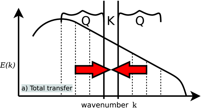
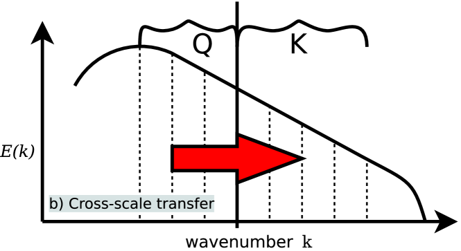
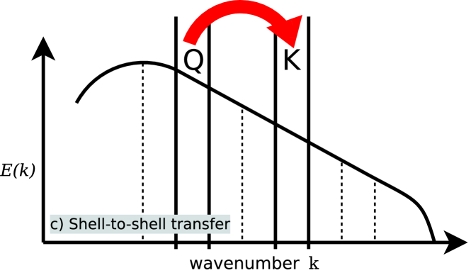
Figure 1: Illustrations of the energy transfers that are analyzed in this paper: a) the total transfer, i.e. energy from all shells going to a particular shell (see III.3), b) cross-scale transfer, i.e. energy from all scales larger than a particular scale going to all scales smaller than that scale (see II.3 and III.2), and c) shell-to-shell transfer, i.e. energy going from a particular shell $Q$ to another shell $K$ (see III.4). Naturally, all shells can be either part of the kinetic or magnetic energy reservoir, which is not further illustrated in the sketch.

The total transfer in (or out) of a shell $\mathrm{K}$ is given by (13) and illustrated in Fig.1a. It can be further separated by looking at an individual shell $\mathrm{Q}$ rather than the sum over all shells as shown in Fig.1c. In the following, we denote individual transfers by

$$\mathcal{T}_{\mathrm{XY}}(Q,K)\quad\text{with}\quad\mathrm{X,Y}\in\{\mathrm{U,B}\}$$ (14)

expressing energy transfer (for $\mathcal{T}_{\mathrm{}}>0$) from shell $\mathrm{Q}$ of energy reservoir $\mathrm{X}$ to shell $\mathrm{K}$ of energy reservoir $\mathrm{Y}$. The kinetic energy reservoir identified by $\mathrm{U}$ is always linked to a shell filtered $\mathbf{w}$ quantity, whereas the magnetic energy reservoir identified by $\mathrm{B}$ is always linked to a shell filtered $\mathbf{B}$ quantity. If a third lower index is present it refers to the mediating force and is not linked to a specific reservoir.

In general, we define all fundamental transfers so that they satisfy antisymmetry

$$\mathcal{T}_{\mathrm{XY}}(Q,K)=-\mathcal{T}_{\mathrm{YX}}(K,Q)\;.$$ (15)

In other words, energy transferred from shell $\mathrm{Q}$ of reservoir $\mathrm{X}$ to shell $\mathrm{K}$ of reservoir $\mathrm{Y}$ is, by definition, equal to the amount of energy received by shell $\mathrm{K}$ of reservoir $\mathrm{Y}$ from shell $\mathrm{Q}$ of reservoir $\mathrm{X}$.

It should be noted that the formalism used here allows one to draw conclusions about the transfer of energy between scales, but not whether this transfer is local or non-local with respect to the mediating mode. From the point of view of triad interactions we generally do not restrict the third, mediating quantity in the transfer functions. For this reason, conclusions on the nature of the interaction – for example, whether it is local or non-local – cannot be easily drawn from analyzing these terms, especially if linearly binned shells are used (Alexakis, Mininni, and Pouquet, 2005; Aluie and Eyink, 2009).

Kinetic cascade terms

The first two terms in the kinetic energy equation (II.1.1) correspond to transfer attributed to the kinetic cascade as they mediate energy transfer within the kinetic energy reservoir. They are given by

$$\mathcal{T}_{\mathrm{UU}}(Q,K)=-\int\underbrace{\mathbf{w}^{\mathrm{K}}\cdot\left(\mathbf{u}\cdot\nabla\right)\mathbf{w}^{\mathrm{Q}}}_{\equiv\mathcal{T}_{\mathrm{UUa}}}+\underbrace{\frac{1}{2}\mathbf{w}^{\mathrm{K}}\cdot\mathbf{w}^{\mathrm{Q}}\nabla\cdot\mathbf{u}}_{\equiv\mathcal{T}_{\mathrm{UUc}}}\mathrm{d}\mathbf{x}\;.$$ (16)

The total term can be further split into an advective component, $\mathcal{T}_{\mathrm{UUa}}$, and a compressive component, $\mathcal{T}_{\mathrm{UUc}}$. The former is equivalently present in incompressible MHD, whereas the latter explicitly captures compressive dynamics. It should be noted, that only the total term $\mathcal{T}_{\mathrm{UU}}$ satisfies antisymmetry and not the individual terms.

Magnetic tension related terms

The third term in the kinetic energy equation (II.1.1) regulates energy transfer from magnetic energy to kinetic energy by magnetic tension. This term in the equation describes energy transfer in the direction of the Alfén wave propagation through tension, and it is given by

$$\mathcal{T}_{\mathrm{BUT}}(Q,K)=\int\mathbf{w}^{\mathrm{K}}\cdot\left(\mathbf{v}_{\mathrm{A}}\cdot\nabla\right)\mathbf{B}^{\mathrm{Q}}\mathrm{d}\mathbf{x}\;.$$ (17)

Here, we applied $\nabla\cdot\mathbf{B}^{\mathrm{Q}}=0$.

It is antisymmetric to the corresponding first term in the magnetic energy equation (II.1.1),

$$\mathcal{T}_{\mathrm{UBT}}(Q,K)=\int\mathbf{B}^{\mathrm{K}}\cdot\nabla\cdot\left(\mathbf{v}_{\mathrm{A}}\otimes\mathbf{w}^{\mathrm{Q}}\right)\mathrm{d}\mathbf{x},$$ (18)

where $\otimes$ denotes a tensor product. By nature of the symmetry, $\mathcal{T}_{\mathrm{UBT}}$ transfers energy from the kinetic energy reservoir to the magnetic one. Here, we replaced the magnetic field and the velocity field by the Alfén velocity and the density weighted velocity, respectively. In addition to satisfying symmetry, this replacement allows for a consistent treatment of the kinetic energy reservoir. In the compressible regime, terms related to normal shell filtered velocities, e.g. $\mathbf{u}^{\mathrm{Q}}$, correspond to the specific kinetic energy. However, we are interested in the dynamics of the energy densities and therefore introduce/replace the appropriate $\mathbf{w}^{\mathrm{Q}}$ where necessary — also in the following equations.

Magnetic pressure and cascade related terms

The last term in the kinetic energy equation (II.1.1) corresponds to changes due to magnetic pressure. We treat this term in a fashion analogous to that proposed by Fromang & PapaloizouFromang, S. and Papaloizou, J. (2007) and Simon et al.Simon, Hawley, and Beckwith (2009), which allows the magnetic pressure to be decoupled from the magnetic cascade dynamics (contrary to the suggestion of Moll et al.Moll et al. (2011)). We proceed by applying shell decomposition directly to the last term in equation (II.1.1):

$$\mathcal{T}_{\mathrm{BUP}}(Q,K)=-\int\frac{\mathbf{w}^{\mathrm{K}}}{2\sqrt{\rho}}\cdot\nabla\left(\mathbf{B}\cdot\mathbf{B}^{\mathrm{Q}}\right)\mathrm{d}\mathbf{x}\;.$$ (19)

In other words, if one factor $B_{j}$ is associated with a shell Q, resulting in ${B}^{\mathrm{Q}}_{j}$, and the other with all mediating modes, $\sum_{\mathrm{P}}{B}^{\mathrm{P}}_{j}=B_{j}$, the product rule for quadratic expressions does not apply to ${B}^{\mathrm{P}}_{j}{B}^{\mathrm{Q}}_{j}$ such that the magnetic to kinetic transfer is given by the above expression. In order to derive the corresponding (antisymmetric) transfer term in the magnetic energy equation, we first expand the original term to

$$\mathrm{Re}\left[-\savestack{\tmpbox}{\stretchto{\scaleto{\scalerel*[\widthof{B_{i}}]{\kern-0.6pt\bigwedge\kern-0.6pt}{\rule[-505.89pt]{4.30554pt}{505.89pt}}}{}}{0.5ex}}\stackon[1pt]{B_{i}}{\tmpbox}\savestack{\tmpbox}{\stretchto{\scaleto{\scalerel*[\widthof{\partial_{j}u_{j}B_{i}}]{\kern-0.6pt\bigwedge\kern-0.6pt}{\rule[-505.89pt]{4.30554pt}{505.89pt}}}{}}{0.5ex}}\stackon[1pt]{\partial_{j}u_{j}B_{i}}{\tmpbox}^{*}\right]=\mathrm{Re}\left[-\savestack{\tmpbox}{\stretchto{\scaleto{\scalerel*[\widthof{B_{i}}]{\kern-0.6pt\bigwedge\kern-0.6pt}{\rule[-505.89pt]{4.30554pt}{505.89pt}}}{}}{0.5ex}}\stackon[1pt]{B_{i}}{\tmpbox}\savestack{\tmpbox}{\stretchto{\scaleto{\scalerel*[\widthof{u_{j}\partial_{j}B_{i}}]{\kern-0.6pt\bigwedge\kern-0.6pt}{\rule[-505.89pt]{4.30554pt}{505.89pt}}}{}}{0.5ex}}\stackon[1pt]{u_{j}\partial_{j}B_{i}}{\tmpbox}^{*}-\savestack{\tmpbox}{\stretchto{\scaleto{\scalerel*[\widthof{B_{i}}]{\kern-0.6pt\bigwedge\kern-0.6pt}{\rule[-505.89pt]{4.30554pt}{505.89pt}}}{}}{0.5ex}}\stackon[1pt]{B_{i}}{\tmpbox}\savestack{\tmpbox}{\stretchto{\scaleto{\scalerel*[\widthof{B_{i}\partial_{j}u_{j}}]{\kern-0.6pt\bigwedge\kern-0.6pt}{\rule[-505.89pt]{4.30554pt}{505.89pt}}}{}}{0.5ex}}\stackon[1pt]{B_{i}\partial_{j}u_{j}}{\tmpbox}^{*}\right]\\ =\mathrm{Re}\left[-\savestack{\tmpbox}{\stretchto{\scaleto{\scalerel*[\widthof{B_{i}}]{\kern-0.6pt\bigwedge\kern-0.6pt}{\rule[-505.89pt]{4.30554pt}{505.89pt}}}{}}{0.5ex}}\stackon[1pt]{B_{i}}{\tmpbox}\savestack{\tmpbox}{\stretchto{\scaleto{\scalerel*[\widthof{u_{j}\partial_{j}B_{i}}]{\kern-0.6pt\bigwedge\kern-0.6pt}{\rule[-505.89pt]{4.30554pt}{505.89pt}}}{}}{0.5ex}}\stackon[1pt]{u_{j}\partial_{j}B_{i}}{\tmpbox}^{*}-\frac{1}{2}\savestack{\tmpbox}{\stretchto{\scaleto{\scalerel*[\widthof{B_{i}}]{\kern-0.6pt\bigwedge\kern-0.6pt}{\rule[-505.89pt]{4.30554pt}{505.89pt}}}{}}{0.5ex}}\stackon[1pt]{B_{i}}{\tmpbox}\savestack{\tmpbox}{\stretchto{\scaleto{\scalerel*[\widthof{B_{i}\partial_{j}u_{j}}]{\kern-0.6pt\bigwedge\kern-0.6pt}{\rule[-505.89pt]{4.30554pt}{505.89pt}}}{}}{0.5ex}}\stackon[1pt]{B_{i}\partial_{j}u_{j}}{\tmpbox}^{*}-\savestack{\tmpbox}{\stretchto{\scaleto{\scalerel*[\widthof{B_{i}}]{\kern-0.6pt\bigwedge\kern-0.6pt}{\rule[-505.89pt]{4.30554pt}{505.89pt}}}{}}{0.5ex}}\stackon[1pt]{B_{i}}{\tmpbox}\savestack{\tmpbox}{\stretchto{\scaleto{\scalerel*[\widthof{B_{i}\partial_{j}\frac{w_{j}}{2\sqrt{\rho}}}]{\kern-0.6pt\bigwedge\kern-0.6pt}{\rule[-505.89pt]{4.30554pt}{505.89pt}}}{}}{0.5ex}}\stackon[1pt]{B_{i}\partial_{j}\frac{w_{j}}{2\sqrt{\rho}}}{\tmpbox}^{*}\right]\;.$$ (20)

The last term in (20) can be associated with transfer from kinetic energy to magnetic energy via magnetic pressure

$$\mathcal{T}_{\mathrm{UBP}}(Q,K)=-\int\mathbf{B}^{\mathrm{K}}\cdot\mathbf{B}\nabla\cdot\left(\frac{\mathbf{w}^{\mathrm{Q}}}{2\sqrt{\rho}}\right)\mathrm{d}\mathbf{x}\;.$$ (21)

Again, this term satisfies antisymmetry with its counterpart (19) within this formulation.

The first two terms in (20) can now be associated with magnetic to magnetic transfer, i.e. a magnetic cascade with

$$\mathcal{T}_{\mathrm{BB}}(Q,K)=-\int\underbrace{\mathbf{B}^{\mathrm{K}}\cdot\left(\mathbf{u}\cdot\nabla\right)\mathbf{B}^{\mathrm{Q}}}_{\equiv\mathcal{T}_{\mathrm{BBa}}}+\underbrace{\frac{1}{2}\mathbf{B}^{\mathrm{K}}\cdot\mathbf{B}^{\mathrm{Q}}\nabla\cdot\mathbf{u}}_{\equiv\mathcal{T}_{\mathrm{BBc}}}\mathrm{d}\mathbf{x}\;.$$ (22)

This term satisfies antisymmetry with itself. Moreover it has the identical shape as $\mathcal{T}_{\mathrm{UU}}$ in the kinetic energy equation and can similarly be split into an advection-related component, $\mathcal{T}_{\mathrm{BBa}}$, and a compression-related component, $\mathcal{T}_{\mathrm{BBc}}$. Again, the advection term is already known from the incompressible MHD regime, whereas the compressive term is new.

It should be noted, that the last two terms in (20) are mathematically identical and that the separation into magnetic pressure and compression stems from chosen shell decomposition of the different variables. This hints at the dual nature of that term and represents our view on separating magnetic cascade dynamics from the energy transfer between kinetic and magnetic budgets as discussed later.

Pressure and external force terms

The two remaining terms in the kinetic energy equation (II.1.1) are not associated with energy transfer between or within kinetic and magnetic energy reservoirs.

First, the pressure gradient term is given by

$$\mathcal{T}_{\mathrm{PU}}(Q,K)=-\int\frac{1}{\sqrt{\rho}}\mathbf{w}^{\mathrm{K}}\cdot\nabla{p}^{\mathrm{Q}}\mathrm{d}\mathbf{x}\;.$$ (23)

It allows for an exchange of energy between the kinetic reservoir and the internal energy reservoir, or, in case of isothermal turbulence, density fluctuations. Given that the present manuscript is primarily concerned with the dynamics within and betweeen kinetic and magnetic energy budgets and that we analyze sub- and mildly supersonic, isothermal turbulence, this term and internal energy dynamics are generally not discussed in great detail.

Second, energy is injected by a mechanical force. The exact shell-to-shell transfer of that external force is given by

$$\mathcal{T}_{\mathrm{FU}}(Q,K)=-\int\sqrt{\rho}\mathbf{w}^{\mathrm{K}}\cdot\mathbf{a}^{\mathrm{Q}}\mathrm{d}\mathbf{x}\;.$$ (24)

It is easily seen that if the force is specified via an acceleration field the density field is acting as a mediator. Some implications of this are discussed in a later section.

Summary

Putting all terms together the interplay of kinetic and magnetic energies in a shell $\mathrm{K}$ is given by

$$\begin{split}\partial_{t}E_{\mathrm{u}}^{\mathrm{K}}=\int\sum_{\mathrm{Q}}\Big{(}&\mathcal{T}_{\mathrm{UUa}}+\mathcal{T}_{\mathrm{BUT}}+\mathcal{T}_{\mathrm{PU}}+\mathcal{T}_{\mathrm{FU}}+\\ &{\color[rgb]{0,0,1}\mathcal{T}_{\mathrm{UUc}}}+{\color[rgb]{0,0,1}\mathcal{T}_{\mathrm{BUP}}}\Big{)}\;\mathrm{d}\mathbf{x}+\mathcal{D}\end{split}$$ (25)

$$\partial_{t}E_{\mathrm{B}}^{\mathrm{K}}=\int\sum_{\mathrm{Q}}\Big{(} \mathcal{T}_{\mathrm{BBa}}+{\color[rgb]{0,0,1}\mathcal{T}_{\mathrm{BBc}}}+\mathcal{T}_{\mathrm{UBT}}+{\color[rgb]{0,0,1}\mathcal{T}_{\mathrm{UBP}}}\Big{)}\;\mathrm{d}\mathbf{x}+\mathcal{D}$$ (26)

where the new terms that enter the formalism in the compressible regime are highlighted in blue. For completeness, we also indicate the numerical dissipation present in the type of simulations we are analyzing by $\mathcal{D}$.

II.2 Definition of shells

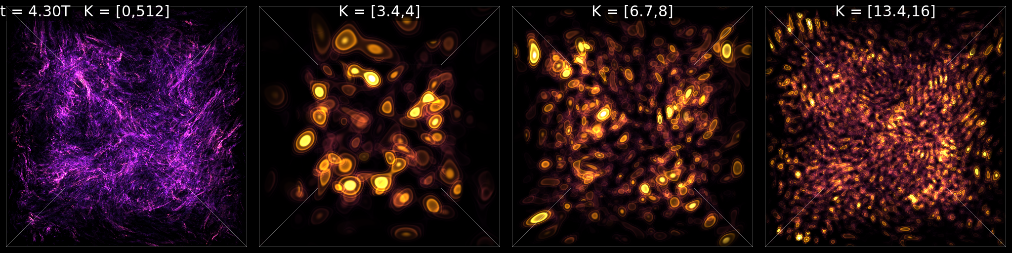
Figure 2: Illustration of eddies of different sizes in real space for the logarithmic binning employed in this paper. Eddies are illustrated based on the Q-criterion Hunt, Wray, and Moin (1988), where $Q=\left(\left\lVert\Omega\right\rVert^{2}-\left\lVert\mathcal{S}\right\rVert^{2}\right)/2$ indicates regions dominated by straining motion for $Q<0$ and regions dominated by rotational motion for $Q>0$. To illustrate eddies we exclude regions with $Q$ smaller than $0.2$ times its standard deviation. Logarithmic binning allows for localized structures in real space.

The definition of the shells in spectral space is an important aspect of this kind of analysis. Different definitions probe different features, particularly if the locality of energy transfer is of concern. For example, linear binning with $K\equiv k\in(\mathrm{K}-0.5,\mathrm{K}+0.5]$ is used(Alexakis, Mininni, and Pouquet, 2005; Moll et al., 2011) and corresponds to space-filling, monochromatic wave-like structures. Another example is octave binning with $K\equiv k\in(K/2,K]$ or more generally logarithmic binning(CARATI et al., 2006; Aluie and Eyink, 2009), which allows for structures, such as eddies, that are simultaneously localized in real and spectral space as illustrated in Fig. 2. Such an approach allows for more physically intuitive interpretations of the turbulent cascade to emerge as it is closer to the phenomenological cascade picture and naturally related to a power-law spectrum. We adopt it here for these reasons.

In particular, our shell boundaries are given by $1$ and $2^{n/4+2}$ for $n\in\{-1,0,1,\ldots,28\}$. They are illustrated by the vertical lines in the bottom panel of Fig. 3.

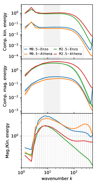
Figure 3: Compensated mean kinetic (top) and magnetic (center) energy spectra over all snapshots of a simulation. The vertical transparent regions around each line illustrate the standard deviation. For most of the lines the variation is very small and the transparent region lies within the linewidth. Grey areas highlight the range of scales ($7<k<30$) where approximately power-law scaling is observed. The kinetic energy is compensated by $k^{4/3}$ and the magnetic energy by $k^{1.7}$. The scale-by-scale ratio (uncompensated) of magnetic to kinetic energy is shown in the bottom panel. Vertical lines in the bottom panel illustrate the binning used throughout the paper.

In order to maintain a close relationship between wavenumber $k$ (in lowercase letters) and shells $K$ (in uppercase letters) we identify shells by the wavenumber they contain. For example, $K=10$ refers to the shell containing $k=10$, i.e. $k\in(9.5,11.31]$.

II.3 Cross-scale energy fluxes

For the description of cross-scale energy fluxes, i.e. fluxes from scales larger than a certain scale $k$ to the scales smaller than $k$ as illustrated in Fig. 1b, we closely follow the exposition of Debliquy, Verma, and Carati (2005) and extend it to the compressible case.

Based on the shell-to-shell energy transfer functions, the forward (large to small scales) cross-scale fluxes are generally given by

$$\Pi^{\mathrm{X}^{<}}_{\mathrm{Y}^{>}}(k)=\sum_{Q\leq k}\sum_{K>k}\mathcal{T}_{\mathrm{XY}}(Q,K)$$ (27)

where $\mathrm{X,Y}\in\{\mathrm{U,B}\}$ again. $\mathrm{X}^{<}$ refers to energy in reservoir $\mathrm{X}$ at wavenumbers smaller than $k$, whereas $\mathrm{Y}^{>}$ refers to energy in reservoir $\mathrm{Y}$ at wavenumbers larger than $k$.

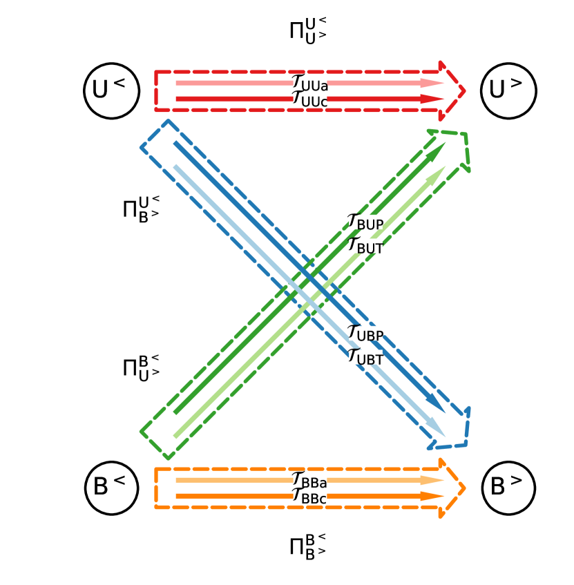
Figure 4: Sketch of the cross-scale energy fluxes between kinetic and magnetic energy reservoirs in ideal compressible MHD. The left spheres correspond to scales larger than a certain scale $k$, whereas the right spheres correspond to smaller scales. Each arrow illustrates transfer by a particular term. Energy fluxes between different reservoirs are mediated by magnetic pressure and tension forces and therefore have two arrows. The $\Pi^{\mathrm{B}^{<}}_{\mathrm{B}^{>}}$ flux (orange arrow) is not present when using variant I of the magnetic pressure formulation.

As in incompressible MHD there are four different cross-scale fluxes in the compressible case between the kinetic and magnetic energy reservoirs as illustrated in Fig. 4. Contrary to incompressible MHD, however, they are not based on four different transfer terms. Here, we have one additional term for each flux. For the intra-reservoir fluxes these are $\mathcal{T}_{\mathrm{UUc}}$ and $\mathcal{T}_{\mathrm{BBc}}$ specifically capturing compressibility effects via $\nabla\cdot\mathbf{u}$. For the inter-reservoir fluxes the additional terms related to magnetic pressure $\mathcal{T}_{\mathrm{BUP}}$ and $\mathcal{T}_{\mathrm{UBP}}$ enter the cross-scale fluxes. They are given as

$$\Pi^{\mathrm{U}^{<}}_{\mathrm{U}^{>}}(k) =\sum_{Q\leq k}\sum_{K>k}\mathcal{T}_{\mathrm{UUa}}(Q,K)+\mathcal{T}_{\mathrm{UUc}}(Q,K)\;,$$ (28)

$$\Pi^{\mathrm{B}^{<}}_{\mathrm{U}^{>}}(k) =\sum_{Q\leq k}\sum_{K>k}\mathcal{T}_{\mathrm{BUT}}(Q,K)+\mathcal{T}_{\mathrm{BUP}}(Q,K)\;,$$ (29)

$$\Pi^{\mathrm{U}^{<}}_{\mathrm{B}^{>}}(k) =\sum_{Q\leq k}\sum_{K>k}\mathcal{T}_{\mathrm{UBT}}(Q,K)+\mathcal{T}_{\mathrm{UBP}}(Q,K)\;,$$ (30)

$$\Pi^{\mathrm{B}^{<}}_{\mathrm{B}^{>}}(k) =\sum_{Q\leq k}\sum_{K>k}\mathcal{T}_{\mathrm{BBa}}(Q,K)+\mathcal{T}_{\mathrm{BBc}}(Q,K)\;.$$ (31)

II.4 Numerical data

Run	Integrator	Riemann solver	$\nabla\cdot\mathbf{B}$	Isothermal EOS	Forcing type	Forcing modes
$\mathtt{M0.5-Enzo}$	MUSCL-Hancock	HLLD	Cleaning	approx.	dynamic	mixed
$\mathtt{M0.5-Athena}$	VL	HLLD	CT	exact	random	solenoidal
$\mathtt{M2.5-Enzo}$	MUSCL-Hancock	HLL	Cleaning	approx.	dynamic	mixed
$\mathtt{M2.5-Athena}$	VL	HLLD	CT	exact	random	solenoidal

Table 1: Overview of the numerical setup for each simulation. More details (including references) are given in the text.

We analyze four datasets of forced, homogeneous, isotropic MHD turbulence. For the purpose of this paper, the datasets can be categorized twofold: by regime and by numerical simulation code (see overview in Table 1). The regime is either approximately incompressible with a subsonic root-mean-square (r.m.s.) Mach number of $\mathrm{M_{s}}\approx 0.5$, or weakly compressible with a supersonic r.m.s. Mach number of $\mathrm{M_{s}}\approx 2.5$. In both regimes, we use the numerical codes Enzo(Bryan et al., 2014) and Athena(Stone et al., 2008) in order to obtain physically similar simulations that differ by the numerical method employed. In all simulations we solve the ideal, compressible MHD equations on a static, periodic grid with $1024^{3}$ points and side length of $1$ in code units.

The Enzo simulations were used before in a priori testing of subgrid-scale models(Grete et al., 2016). They use the MUSCL-Hancock framework with second-order Runge-Kutta time integration and the HLLD (in the subsonic regime) or HLL (in the supersonic regime) Riemann solver(Wang and Abel, 2009). The gas is kept approximately isothermal by using an adiabatic equation of state with $\gamma=1.001$. The divergence constraint $\nabla\cdot\mathbf{B}=0$ is maintained by hyperbolic divergence cleaning(Dedner et al., 2002).

In the Athena simulations we employ the second-order van Leer integrator(Stone and Gardiner, 2009) with HLLD Riemann solver in both regimes and first-order flux correction. Here, we use an exact isothermal equation of state. Moreover, $\nabla\cdot\mathbf{B}=0$ is maintained to machine precision by using constrained transport.

All simulations start with uniform initial conditions, i.e., $\rho_{0}=1$, $\mathbf{u}_{0}=\mathbf{0}$, and $\mathbf{B}_{0}=\left(0,0,\sqrt{2\rho_{0}c_{\mathrm{s}}^{2}/\beta_{\mathrm{p}}}\right)$, with the speed of sound $c_{\mathrm{s}}=1$ in code units. The initial plasma beta is $\beta_{\mathrm{p}}=72$ in the subsonic regime and $\beta_{\mathrm{p}}=5$ in the supersonic regime, so that turbulence is super-Alfénic in the stationary regime.

Stationary turbulence is reached by constantly forcing the simulation box. We employ an acceleration field with a parabolic shape in spectral space. It peaks at low wavenumbers $k_{0}=2$ and is constrained to modes with $\mathbf{k}\in]0,2k_{0}[$. This translate to a characteristic (or integral) length scale of $L=2$.

In Enzo we use a stochastic acceleration field that evolves in space and time as an Ornstein–Uhlenbeck process(Schmidt et al., 2009). The forcing modes are projected from spectral to real space so that they are split into 50% compressive and 50% solenoidal modes. In Athena we use a random acceleration field that is purely solenoidal. It is regenerated every $0.2T$ large-eddy turnover times.

In general, we follow the simulations for a total of $5T$ turnover times with $T=L/V$. The characteristic velocity $V$ is given by the r.m.s. Mach number in the stationary regime, i.e. $0.5$ in the subsonic case and $2.5$ in the supersonic case. We disregard data during the initial $2T$ where turbulence develops from the uniform initial conditions. During the stationary regime $2T\leq t\leq 5T$ we captures 31 snapshots equally spaced in time. If not otherwise noted, all quantities in the following analysis are given by the mean values over these 31 snapshots and variations given by one standard deviations.

III Results

The results presented here highlight the uses of the analysis technique. In order to get a comprehensive picture of the energy transfers, we start from an aggregated point of view and then go into more and more detail. First, we compare general flow properties and energy spectra as a basis for the discussion. Second, we analyze the energy fluxes across scales. Third, we describe the total transfer, i.e. how much energy is gained (or lost) at a particular scale. Finally, we describe the individual shell-to-shell transfers.

III.1 Flow properties and energy spectra

Run	$\langle E_{\mathrm{u}}\rangle$	$\langle E_{\mathrm{B}}\rangle$	$\langle E_{\mathrm{B}}\rangle/\langle E_{\mathrm{u}}\rangle$	$\langle\beta_{\mathrm{p}}\rangle$	$\langle\langle\mathrm{M}_{\mathrm{s}}^{2}\rangle^{1/2}\rangle$	$\langle\langle\mathrm{M}_{\mathrm{a}}^{2}\rangle^{1/2}\rangle$	$\left<\Pi\right>$
$\mathtt{M0.5-Enzo}$	0.16	0.21	1.36	23.09	0.57	1.81	0.352
$\mathtt{M0.5-Athena}$	0.13	0.16	1.22	27.35	0.51	1.89	0.246
$\mathtt{M2.5-Enzo}$	2.88	2.39	0.83	1.34	2.51	2.11	24.3
$\mathtt{M2.5-Athena}$	3.30	2.78	0.84	1.09	2.63	1.95	37.7

Table 2: Overview of the flow properties, i.e. mean kinetic energy $E_{\mathrm{u}}$, mean magnetic energy $E_{\mathrm{B}}$, ratio of mean magnetic to kinetc energy, mean plasma $\beta_{\mathrm{p}}$, rms sonic Mach number $\mathrm{M_{s}}$ and rms Alfvènic Mach number $\mathrm{M_{a}}$, in the simulations during the stationary phase. The last column lists the mean (over time) of the mean total fluxes (in the inertial range), which are used for normalization in manuscript.

Table 2 shows mean and root mean square (rms) characteristic flow quantities during in the stationary regime. The two simulations in each regime are very similar independent of the numerical method. In the subsonic regime, the rms sonic Mach number is $\approx 0.5$ and the mean plasma $\beta_{\mathrm{p}}$ is $\approx 25$. In the supersonic regime, the sonic Mach number is $\approx 2.5$ and $\beta_{\mathrm{p}}$ of order unity. All simulations are in the super Alfénic regime with rms Alfén Mach number $\approx 2$. While there is more energy in the magnetic reservoir than in the kinetic reservoir in the subsonic regime ($\langle E_{\mathrm{B}}\rangle/\langle E_{\mathrm{u}}\rangle\approx 1.3$), the opposite is true in the supersonic regime where the ratio is $\approx 0.83$.

The larger ratio in the subsonic regime is also present on all scales as shown in the bottom panel of Fig. 3 where the ratio is plotted over wavenumber. In the subsonic regime magnetic energy is dominant on all scales beyond the forcing range. In the supersonic regime it is only dominant beyond the large scale forcing and up to $k\approx 30$. This range coincides with the range where approximately power-law scaling is observed in the kinetic energy spetrum, as can be seen in the top panel of Fig. 3. All simulations have a flat kinetic energy spectrum between $7\lesssim k\lesssim 30$ when compensated by $k^{4/3}$. For this reason, we use this region as the “inertial range” in the following analysis. The compensated (by $k^{1.7}$) magnetic energy spectra in the center panel lack any clear power-law regime, a result that is independent of regime and numerical method and in agreement with previous studiesKritsuk et al. (2011); Porter, Jones, and Ryu (2015).

Overall the spectra are again very similar within each regime and differences due to the numerical method become first apparent at the smallest scales. For example, the supersonic Enzo simulation is the only simulation that uses the HLL Riemann solver, whereas the other three runs use the less dissipative HLLD Riemann solver. This translates to a more pronounced decay of the spectrum at high wavenumbers and a slight decrease of the intertial range. Similarly, differences close to the grid scale are visible in all simulations, especially in the ratio of magnetic to kinetic energy. This is no surprise as this region is dominated by the numerical method itself. For the purpose of the manuscript and our analysis this is of no importance as contributions from these scales are negligible.

III.2 Cross-scale energy fluxes

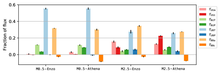
Figure 5: Mean fraction of the cross-scale flux in the inertial range by the individual terms in the stationary phase. The black lines at the end of each block indicate the standard deviation over time. The fluxes have been normalized to sum up to $1$.

We begin the energy transfer analysis from a broad point of view: the mean cross-scale energy flux within the inertial range as illustrated in Fig. 5. We follow the normalization of Debliquy et al.Debliquy, Verma, and Carati (2005). Thus, each snapshot is normalized to the mean total flux in the inertial range

$$\begin{split}\left<\Pi\right>=\sum_{k\in[7,30]}&\Big{(}\Pi^{\mathrm{U}^{<}}_{\mathrm{U}^{>}}(k)+\Pi^{\mathrm{U}^{<}}_{\mathrm{B}^{>}}(k)+\Pi^{\mathrm{B}^{<}}_{\mathrm{U}^{>}}(k)+\\ &\Pi^{\mathrm{B}^{<}}_{\mathrm{B}^{>}}(k)+\Pi^{\mathrm{P}^{<}}_{\mathrm{U}^{>}}(k)+\Pi^{\mathrm{F}^{<}}_{\mathrm{U}^{>}}(k)\Big{)}\;.\end{split}$$ (42)

We use this normalization for all quantities throughout the manuscript, i.e. all transfer functions for a particular snapshot are divided by the respective $\left<\Pi\right>$ of that snapshot. Overall there is little variability with respect to time. In the subsonic regime the cross-scale flux is dominated by kinetic to magnetic transfer by magnetic tension (contributing approximately $55\%$) and magnetic to magnetic transfer by advection ($\approx 31\%$). The contribution of the kinetic cascade is negligible and there is only a limited energy flux from magnetic energy at large scale to smaller scales by magnetic tension ($\approx 11\%$) and magnetic pressure ($\approx 4\%$ for Enzo and $\approx 8\%$ for Athena). It should be noted that these fractions are very close the results obtained by Debliquy et al. (see Table I in Ref. Debliquy, Verma, and Carati, 2005). For example, they report fluxes by magnetic tension of $49\%$ from the kinetic to the magnetic budget and of $12\%$ from the magnetic to the kinetic budget. In addition, their kinetic flux by advection is similarly small ($7.5\%$) and the magnetic flux by advection contributues with $37\%$. Contrary to the compressible finite volume codes we use, they employed a fully-dealiased pseudospectral code and analyzed decaying incompressible MHD turbulence at a resolution of $512^{3}$.

The differences between the subsonic and the supersonic regime are visible upon first inspection. While the magnetic cascade fluxes are unchanged, the contribution of kinetic to magnetic cross-scale flux by magnetic tension is cut in half to about $26\%$. This is generally compensated by the kinetic cascade fluxes even though they vary slightly between Enzo (with $15\%$ by advection and $8.4\%$ by compression) and Athena with $12.7\%$ and $22.4\%$, respectively). Moreover, magnetic pressure now contributes with $\approx 7\%$ to a large scale magnetic to small scale kinetic energy flux, which was absent in the subsonic regime. Overall the picture in the supersonic regime is much more balanced between the individual mediators and there is no single dominant contribution.

One interesting feature in the mean cross-scale fluxes is the magnetic cascade term mediated by compressive effects. One the one hand it is consistently negative, i.e. there is a magnetic energy flux from small to large scales, in all simulations. In the other hand, its seems to be more affected by the numerical method rather than the regime. For Enzo it contributes about $-2.5\%$ in both regimes, whereas for Athena it is more pronounced with approximately $-8\%$.

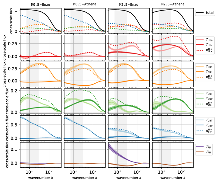
Figure 6: Mean cross-scale fluxes versus wavenumber of the individual terms during the stationary phase. Variations by means of the standard deviation are shown by the vertical shaded regions. The first row includes the joint fluxes between kinetic and magnetic energy reservoirs and the total cross-scale flux for comparison. The total cross-scale flux from large scale kinetic energy to kinetic energy on smaller scales ($\Pi^{\mathrm{U}^{<}}_{\mathrm{U}^{>}}$, second row), large scale magnetic to small scale magnetic ($\Pi^{\mathrm{B}^{<}}_{\mathrm{B}^{>}}$, third row), large scale magnetic to small scale kinetic ($\Pi^{\mathrm{B}^{<}}_{\mathrm{U}^{>}}$, fourth row) and large scale kinetic to small scale magnetic ($\Pi^{\mathrm{U}^{<}}_{\mathrm{B}^{>}}$, fifth row) are highlighted by a dashed line. For completeness, the bottom row shows the cross-scale flux by pressure variations and by the external forcing (data only available in Enzo).

A more detailed picture of the cross-scale fluxes is shown in Fig. 6, where the fluxes are now plotted over all wavenumbers. For all simulations the general shape of the individual fluxes is similar. It is predominately the scale that varies between regimes. It is important to note that the joint total fluxes by all terms together are approximately constant (black lines in the top row) until the end of the inertial range (highlighted by the gray areas). This is expected from theory for an inertial range in the incompressible regime. However, the individual fluxes are not at all constant and change substantially with $k$. For example, the dominant contribution of $\mathcal{T}_{\mathrm{UBT}}$ in the subsonic regime is constantly decreasing within the inertial range whereas the contribution by $\mathcal{T}_{\mathrm{BBa}}$ is constantly increasing.

Overall the contribution of $\mathcal{T}_{\mathrm{BBa}}$ is very robust with respect to shape and magnitude as illustrated in row 3 of Fig. 6. Its contribution is doubling from $\approx 16\%$ at the largest scales to $\approx 32\%$ at the end of the inertial range where it is then damped by numerical dissipation. The previously observed mean inverse flux in the magnetic cascade term via compression $\mathcal{T}_{\mathrm{BBc}}$ in the inertial range now clearly extends beyond the wavenumbers $7<k<30$. It is also more pronounced in the Athena simulations independent of the regime.

This feature is similarly present in the kinetic cascade term via compression $\mathcal{T}_{\mathrm{UUc}}$, which is, albeit having the same shape, 2.5-3 times as strong in M2.5-Athena than it is in M2.5-Enzo. As expected this term is practically absent on all scales in the subsonic regime and independent of numerical method. In general, the cross-scale fluxes from kinetic energy at large scales ($\Pi^{\mathrm{U}^{<}}_{\mathrm{U}^{>}}$ and $\Pi^{\mathrm{U}^{<}}_{\mathrm{B}^{>}}$) exhibit the largest quantitative changes going from the subsonic to the supersonic regime.

Another interesting feature concerns the large scale magnetic to small scale kinetic cross-scale energy transfer $\Pi^{\mathrm{B}^{<}}_{\mathrm{U}^{>}}$ and its components $\mathcal{T}_{\mathrm{BUT}}$ and $\mathcal{T}_{\mathrm{BUP}}$ (see row 4 of Fig. 6). While in the subsonic regime the magnetic tension related flux is consistently non zero up to the smallest scales in the domain, it is effectively zero beyond the inertial range in the supersonic regime. This leads to interesting dynamics in combination with the flux by magnetic pressure. Given that latter is always non zero and positive, the dominant contribution to $\Pi^{\mathrm{B}^{<}}_{\mathrm{U}^{>}}$ changes with scale and in the supersonic regime changes within the inertial range from tension dominated to pressure dominated.

Finally, the direct cross-scale transfer by the external mechanical driving is of importance. Independently of defining an acceleration field, as done here, see (24), or defining a forcing field, the external driving is always coupled to density field. Thus, our acceleration field, which is confined to $k\in]0,4[$, actually injects energy beyond $k=4$. This is most obvious in the bottom row of Fig. 6 where the cross-scale fluxes for the Enzo simulations are plotted. In the subsonic regime it is practically zero on all scales whereas in the supersonic regime it constantly decreases from the largest scales down to $k\approx 100$. It is directly linked to the different extent of density fluctuations between the sub- and the supersonic regime. We only have data available for the Enzo simulation. The absence of that term is clearly visible for the total cross-scale flux in M2.5-Athena, which is not constant (in our analysis) on the largest scales for that reason.

III.3 Total energy transfer

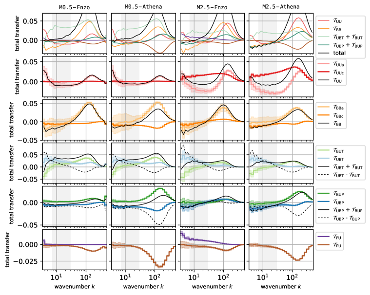
Figure 7: Mean total transfer in (positive) or out (negative) of a shell from (or to) all other shells. The transparent regions show the standard deviation over time. For comparison, all transfers including the total transfer are illustrated in the first row. The second row shows transfer from the kinetic energy reservoir to kinetic energy on other scales, the third row magnetic to magnetic transfer, the fourth row magnetic to kinetic transfer and the fifth row kinetic to magnetic transfer. The bottom row shows the transfers that are not within or between kinetic and magnetic energies, i.e. transfer by the external force (data only available for Enzo) and pressure. The dashed lines in the magnetic tension and pressure related panels illustrate the net transfer to magnetic energy. All transfer functions follow the same normalization as before, i.e. they are normalized by the total mean inertial cross-scale flux $\left<\Pi\right>$.

After the presentation of the energy transfer across scales, we now present the total energy transfer into and out of particular scales, i.e. $\sum_{Q}\mathcal{T}_{\mathrm{}}(Q,K)$. Figure 7 illustrates these transfers for all terms over all wavenumbers beyond the direct forcing regime. As with the cross-scale fluxes the overall picture is qualitatively very similar across the simulations, but has some notable quantitative differences.

The kinetic cascade term $\mathcal{T}_{\mathrm{UU}}$ is approximately zero within the inertial range. However, there are significant differences between the subsonic and supersonic regimes. While in the former regime both contributions ($\mathcal{T}_{\mathrm{UUa}}$ and $\mathcal{T}_{\mathrm{UUc}}$) are effectively zero, they are negative (advective term) and positive (compressive term) in the supersonic regime. Thus, compression and advection work against each other and their contributions cancel.

Similarly, the magnetic cascade term is approximately zero within the inertial range, but the individual terms are practically identical in both regimes. The advective component $\mathcal{T}_{\mathrm{BBa}}$ exhibits large variations around zero throughout the inertial range whereas the compressive component $\mathcal{T}_{\mathrm{BBc}}$ is constantly negative with only little variability.

The magnetic tension related terms ($\mathcal{T}_{\mathrm{BUT}}$ and $\mathcal{T}_{\mathrm{UBT}}$) provide an interesting insight into the dynamics between kinetic and magnetic energies. On the one hand, their joint effect leads to an increase of the total energy on all scales (see solid black line in the fourth row of Fig. 7). On the other hand, that increase of total energy is in magnetic energy on large and intermediate scales (positive dashed black line) and in kinetic energy on smaller scales (negative dashed black line). The zero crossing takes place at the end of the inertial range in all simulations. Whether this occurs by coincidence or due to the underlying physics should be verified in additional simulations at different resolutions. Moreover, this profile is also quantitatively fairly independent of the regime and numerical method.

Transfers mediated by magnetic pressure show a less consistent picture between individual runs, see fifth row of Fig. 7. In the supersonic regime the variations in both terms throughout the inertial range are consistent with zero. In the subsonic regime there is less variability and the kinetic to magnetic transfer $\mathcal{T}_{\mathrm{UBP}}$ is clearly negative and slight more pronounced in the Athena simulation. Interestingly, magnetic pressure is thus working against magnetic tension in transferring energy from the kinetic reservoir to the magnetic one within the inertial range as $\mathcal{T}_{\mathrm{UBT}}$ is positive over these wavenumbers.

As already seen in the cross-scale transfers, the forcing term is non-zero beyond the direct forcing scales (bottom row of Fig. 7) in the supersonic regime. Even though its overall contribution is weak, some energy is directly injected to the kinetic reservoir on intermediate scales.

Finally, two additional features should be noted. First, the profile of the total transfer of all terms (black line in the top row of Fig. 7) starts to deviate from zero beyond the inertial range. This is a direct measure of the numerical dissipation of the individual numerical methods. Second, from a total transfer point of view $\mathcal{T}_{\mathrm{BBc}}$ and $\mathcal{T}_{\mathrm{UBP}}$ are almost identical. Similarly, $\mathcal{T}_{\mathrm{BBa}}$ and $\mathcal{T}_{\mathrm{BUP}}$ exhibit the same dynamics. This can be related to their derivation, see (20) and (21). However, this impression is misleading as their underlying shell-to-shell transfer is different as shown in the following subsection.

III.4 Shell-to-shell transfer

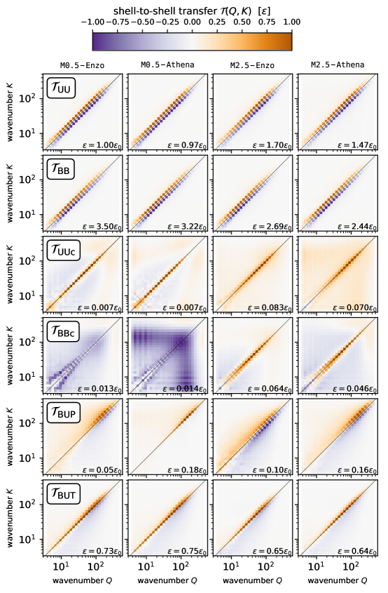
Figure 8: Mean transfer from shell $Q$ to shell $K$ by the individual transfer terms (from top to bottom): $\mathcal{T}_{\mathrm{UU}}$, $\mathcal{T}_{\mathrm{BB}}$, $\mathcal{T}_{\mathrm{UUc}}$, $\mathcal{T}_{\mathrm{BBc}}$, $\mathcal{T}_{\mathrm{BUP}}$ and $\mathcal{T}_{\mathrm{BUT}}$. The transfers for $\mathcal{T}_{\mathrm{UBP}}$ and $\mathcal{T}_{\mathrm{UBT}}$ are not explicitly shown. Due to the antisymmetry property their illustrations are are identical to the transposed panels of the shown $\mathcal{T}_{\mathrm{BUP}}$ and $\mathcal{T}_{\mathrm{BUT}}$ terms, respectively. Each panel uses a unique symmetric colorbar that extends from $-\varepsilon$ to $\varepsilon$. All are normalized to the maximum $\mathcal{T}_{\mathrm{UU}}$ value of simulation M0.5-Enzo with $\varepsilon_{0}=0.052$.

We close the analysis section with the presentation of the individual shell-to-shell transfers for all terms as depicted in Fig. 8.

In agreement with earlier work, we find the kinetic $\mathcal{T}_{\mathrm{UU}}$ and magnetic $\mathcal{T}_{\mathrm{BB}}$ cascade transfer function to be highly local, as shown in panels in the top two rows of Fig. 8. Independent of regime and numerical method, energy is received from the next shell on larger scales and released to the next shell on smaller scales. While in the subsonic regime the magnetic cascade is more than three times as strong as the kinetic cascade, it is a little more balanced in the supersonic regime. Here, the kinetic cascade is $\approx 1.6$ stronger compared to the M0.5 runs and the magnetic cascade is less than twice as strong as its kinetic counterpart as indicated by the different scaling coefficient $\epsilon$. In general, each panel is normalized with an individual $\epsilon$, see caption of Fig. 8.

The compressive $\mathcal{T}_{\mathrm{XXc}}$ components of $\mathcal{T}_{\mathrm{UU}}$ and $\mathcal{T}_{\mathrm{BB}}$ are plotted in rows three and four of Fig. 8. The kinetic compressive component is overall quite consistent between numerical methods. However, going from the M0.5 to M2.5 increases its strength by a factor of $10$ even though it is overall still weak compared to the full cascade term $\mathcal{T}_{\mathrm{UU}}$. The full term is zero on the diagonal, i.e. $K=Q$ by construction. This is not true of its components and $\mathcal{T}_{\mathrm{UUc}}$ is actually strongest (and positive) on the diagonal. Conversely, $\mathcal{T}_{\mathrm{UUa}}$ (not shown) must be negative on the diagonal illustrating how advection and compression work against each other as already mentioned.

The compressive magnetic cascade term $\mathcal{T}_{\mathrm{BBc}}$ is in stark contrast to its kinetic counterpart. The regime plays an important role. For both subsonic runs the transfer is entirely negative independent of the giving and receiving wavenumber. Moreover, the numerical method also introduces differences. In M0.5-Enzo the transfer predominately takes place off the diagonal and between large scales whereas in M0.5-Athena the strongest transfers are on the small scales. In the supersonic regime the picture is more consistent with respect to codes. Contrary to the subsonic regime, energy is now received from shells on and adjacent to a particular shell $K$, and transfers that are not close to the diagonal are comparatively weak.

As mentioned in the previous subsection, magnetic pressure and magnetic cascade transfers seem to be almost identical from a total transfer point of view. However, the individual shell-to-shell analysis (see fifth row of Fig. 8) reveals that $\mathcal{T}_{\mathrm{BUP}}$ is much less localized in spectral space. Energy is now transferred not only between the next larger and smaller shell, but also between the next 3-4 shells in both directions. In addition, a difference in the numerical methods is seen in the (numerically) dissipative regime. Independent of regime, there is no significant transfer of energy between kinetic and magnetic energies at the same scale ($K=Q$) for Enzo. In Athena a non negligible amount of energy is transfered from magnetic to kinetic energy at the same scale. This transfer is overall the strongest transfer mediated by magnetic pressure in the subsonic regime.

Finally, the shell-to-shell transfer via magnetic tension is in agreement with previous results(Aluie and Eyink, 2010; Teaca, Carati, and Domaradzki, 2011). It is weakly local and also most pronounced on the diagonal, i.e. energy is directly transferred between magnetic and kinetic reservoirs at the same scale. Moreover, this feature is consistent between regimes (with less than $20\%$ difference in strength) and independent of numerical method.

IV Discussion

The energy dynamics presented in Section III provide an interesting insight into both compressible MHD turbulence dynamics and numerics. For example, our results in the subsonic regime are in good agreement with previous studies conducted in the incompressible MHD regimeDebliquy, Verma, and Carati (2005); Aluie and Eyink (2010); Teaca, Carati, and Domaradzki (2011). This agreement is even more relevant given that these studies employed a spectral code whereas we employ fully compressible finite volume codes. However, subtle differences between the two methods we used are revealed by the analysis, e.g., for the inverse fluxes of the compressible magnetic cascade term on the smallest scales. A more detailed study of the presented energy dynamics in identical setups with different numerical methods including spectral and finite difference methods would be informative. Such an analysis would allow for the quantification of the practical influence of the numerical scheme on the dynamics and a measurement of numerical dissipation similar to Salvesen at al.Salvesen et al. (2014).

The observed upscale flux in the compressible magnetic cascade term is also relevant for subgrid-scale models in large eddy simulationsMiesch et al. (2015). Purely dissipative models, such as an eddy viscosity or resistivity, are prone to overestimate the downscale flux. Structural models, e.g. the nonlinear model by Vlaykov et al.Vlaykov et al. (2016) that explicitly captures compressibility effects in MHD, are capable of reproducing inverse fluxesGrete et al. (2016). The local nature of the energy transfer in the kinetic and magnetic cascade terms seems to be ideally suited for scale similarity-type subgrid-scale modelsBardina, Ferziger, and Reynolds (1980). However, Grete et al. (2017)Grete et al. (2017) showed that contrary to the nonlinear model, the scale similarity model did not improve higher order statistics when applied to decaying, supersonic MHD turbulence.

From an energy transfer point of view, our extension of the shell-to-shell analysis method to the compressible regime allows for a separation of a magnetic cascade and transfer by magnetic pressure, see II.1.3. On the one hand some previous studies claimedGraham, Cameron, and Schüssler (2010); Moll et al. (2011) that magnetic energy transfer between different scales (the magnetic cascade) and the exchange of energy between kinetic and magnetic reservoirs via magnetic pressure cannot be separated. On the other hand this separation has already been shown in the context of total transfer functionsSimon, Hawley, and Beckwith (2009). Here, we go one step further and split the total transfer functions into shell-to-shell transfer functions. This view allowed us to illustrate that the magnetic cascade is quite different from the magnetic pressure related terms at a shell-to-shell level. For example, $\mathcal{T}_{\mathrm{BBc}}$ and $\mathcal{T}_{\mathrm{UBP}}$ are identical at the level of total energy transfers. However, from an individual shell-to-shell point of view they are very dissimilar.

Another important result revealed by the analysis concerns the external force used in driven turbulence simulations. The forcing (or acceleration) field is inescapably coupled to the density field. This is of no concern in the subsonic regime due to limited density fluctuations. While the supersonic regime in our simulations is only mildly supersonic with $\mathrm{M_{s}}\approx 2.5$, we already observe a non-negligible energy input throughout the inertial range. On the one hand, this effect, i.e. energy injection beyond the range of scales defined in the external field, is expected to be much more pronounced in the highly supersonic regime. On the other hand, AluieAluie (2013) proved in the context of a Favre filtering based scale decomposition that transfers via the forcing term vanish for $K\gg Q$. This is also observed in our approach, see Fig. 7. Overall, analyzing driven turbulence data in highly supersonic regimes (e.g., with respect to slopes of the spectral energy densities) should thus be done with special care, especially in presence of a limited inertial range.

Moreover, Domaradzki et al.Domaradzki, Teaca, and Carati (2010) showed that even in the incompressible MHD regime the directly forced scales implicitly affect the transfer functions. Even though there is no direct energy injection by the $\mathcal{T}_{\mathrm{FU}}$ function beyond the forced scales, the nature of triadic interactions allow for the mediator to lie within the forced scales. The latter typically contain the most power and carry an imprint of the external forcing field. Thus, individual triadic interactions between (typically weaker) small scales are affected by a leg in the forced scales. It is a natural effect occurring in all forced turbulence simulations. In this manuscript, we are not concerned with individual interactions but use mediators that contain information of all wave numbers, which always include interactions with the forcing scales. The same approch is used by Domaradzki et al.Domaradzki, Teaca, and Carati (2010) and they estimate a minimum resolution well above $1000^{3}$ in order to see a decoupling of the forcing scales from the smallest resolved scales. While the resolution of our simulations is close to that number, we expect it to be greater in the case of compressible MHD (with shock-capturing finite volume methods) — especially if more than the smallest resolved scales should be decoupled.

In addition to the forcing, several other characteristics of our present analysis should be kept in mind. For example, the third quantity in the transfer functions is not restricted to a particular scale. As noticed by Alexakis et al.Alexakis, Mininni, and Pouquet (2005), this translates to all transfer functions containing information only about whether the energy transfer itself is local and not about whether the interaction itself is local. However, as pointed out by Aluie & EyinkAluie and Eyink (2010) the choice of the shell spacing directly influences whether local or nonlocal interaction are favored. For the logarithmic binning we use the number of possible local interactions is much larger than the number of possible nonlocal interaction. Thus, our results may also be interpreted as a hint about the locality of the interactions, but a more detailed study is required. Similarly, the present study is concerned with one of the simpler MHD turbulence configurations (super-Alfvénic, isotropic, non helical) as a proof of concept for the analysis. Again follow-up studies in different regimes, such as turbulence with a strong background magnetic field or in the presence of an inverse magnetic helicity cascade, are desirable.

V Conclusions

In this paper we extended an established shell-to-shell energy transfer analysis to the compressible MHD regime. Four transfer functions regulating energy transfer within and between kinetic and magnetic reservoirs are known from the incompressible formalism: kinetic to kinetic transfer by advection (the kinetic cascade), magnetic to magnetic transfer (the magnetic cascade), and transfer from kinetic to magnetic energy (and vice versa) by magnetic tension. We derived four additional terms are present in the compressible formalism that can be separated into two categories. First, both known cascade functions now contain not only the advective term but also a second term directly associated with the compressibility $\nabla\cdot\mathbf{u}$ . Second, an additional channel to exchange energy between kinetic and magnetic reservoirs is possible. We interpret this channel as mediated by magnetic pressure, which adds two (antisymmetric) transfer functions.

In order to illustrate the value of this formalism, we conducted and analyzed four simulations of driven, isothermal, ideal MHD turbulence. Using two different numerical codes, Enzo and Athena, in two regimes, subsonic ($\mathrm{M_{s}}\approx 0.5$) and supersonic ($\mathrm{M_{s}}\approx 2.5$), we were able to identify similarities and differences both with respect to MHD turbulence and numerical method.

In addition to the pure shell-to-shell transfer we also analyzed higher-level transfers, e.g. energy transfer across scale and the total transfer into (or out of) specific scales by the individual functions. Differences between regimes became apparent. While the cross-scale fluxes in the subsonic regime are dominated by kinetic to magnetic energy transfer via tension and magnetic to magnetic transfer via advection, the supersonic regime provides a more diverse impression. In this regime, kinetic to kinetic transfer by both advection and compression and kinetic to magnetic transfer via magnetic pressure contribute with non-negligible amounts. From a total transfer point of view the net effect of the kinetic cascade is similar in both regimes. Despite similarity in the net effect, while in the subsonic regime the compressive component is effectively absent in the supersonic regime both advective and compressive transfer are much stronger but also work against each other. The shell-to-shell results are also in agreement with previous findings. Kinetic and magnetic energy both exhibit features of a forward local energy cascade. Nonetheless, it is important to mention that this only holds for the functions that contain the advection and the compressive component. As known from the incompressible regime magnetic tension-related functions are weakly local and forward. Our analysis shows that this is also true for the new magnetic pressure-related functions.

Overall the application of shell-to-shell energy transfer analysis exposed several interesting features that would benefit from more detailed follow-up studies. For example, the dynamics of the compressive component in the magnetic cascade term concerning cross-scale fluxes seem to be dominated by numerical method rather than physical regime. Then again, the dynamics of that term concerning shell-to-shell transfer are quite similar between methods but differ a lot between regimes. Another example is the magnetic to kinetic cross-scale flux. It is dominated by magnetic tension on the large scales and dominated by magnetic pressure on the small scales. There are indications for a trend in characteristic features, e.g. the scale where both are equally strong or where magnetic tension becomes completely negligible, but more data (with different parameters) is required to draw definite conclusions. This also applies to the net total transfer by magnetic tension. In all simulations independent of regime and method the scale where predominately kinetic to magnetic transfer changes to predominately magnetic to kinetic transfer coincides with the end of the inertial range. Here, higher resolution simulations would allow one to trace that behavior in the presence of an extended inertial range.