Efficient and Accurate Machine-Learning Interpolation of Atomic Energies in Compositions with Many Species

Abstract

Machine-learning potentials (MLPs) for atomistic simulations are a promising alternative to conventional classical potentials. Current approaches rely on descriptors of the local atomic environment with dimensions that increase quadratically with the number of chemical species. In this article, we demonstrate that such a scaling can be avoided in practice. We show that a mathematically simple and computationally efficient descriptor with constant complexity is sufficient to represent transition-metal oxide compositions and biomolecules containing 11 chemical species with a precision of around 3 meV/atom. This insight removes a perceived bound on the utility of MLPs and paves the way to investigate the physics of previously inaccessible materials with more than ten chemical species.

Atomic interaction potentials based on the interpolation of first-principles calculations with machine-learning algorithms have the potential to enable efficient linear-scaling atomistic simulations with an accuracy that is close to the reference method Lorenz et al. (2004); Behler and Parrinello (2007); Bartók et al. (2010); Rupp et al. (2012). Such machine-learning potentials (MLPs) establish a relationship between a unique descriptor and the total or atomic energy using, e.g., artificial neural networks (ANNs) Montavon et al. (2012) or Gaussian process regression (GPR, Kriging) Rasmussen and Williams (2006). However, the combined space of atomic coordinates and chemical species grows rapidly with the number of chemical species, resulting in a formal corresponding growth of the descriptor complexity and thus the complexity of the MLP. This scaling has so far limited current MLP approaches to compositions with only a few chemical species Artrith et al. (2011); Artrith and Kolpak (2014, 2015); Morawietz et al. (2016) or atomic structures Faber et al. (2016). Overcoming this limitation is a very active field of research Huo and Rupp (2017); De et al. (2016).

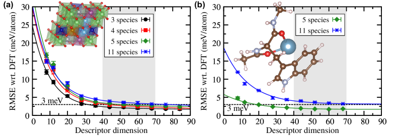
Figure 1: Precision of artificial neural network (ANN) potentials as function of the dimension of the descriptor used to represent the local atomic environment. (a) Root mean squared error (RMSE) of the ANN potential energies relative to their DFT references for Li$M$O2 systems with increasing number of chemical species: 3 species ($M$ = Ti; black circles), 4 species ($M$ = Ti, Ni; red squares), 5 species ($M$ = Ti, Mn, Ni; green diamonds), and 11 species ($M$ = Sc, Ti, V, Cr, Mn, Fe, Co, Ni, Cu; blue stars). The unit cell of a representative Li$M$O2 structure from the data set is shown as inset. (b) An equivalent analysis for a data set with conformations of the 20 proteinogenic amino acids (5 chemical species: H, C, N, O, S; green diamonds) and their complexes with the divalent cations Ba^2+, Ca^2+, Cd^2+, Hg^2+, Pb^2+, Sr^2+ (in total 11 species; blue stars). The inset shows one conformation of a tryptophan dipeptide complex with Ca^2+. Generally, the RMSE was evaluated after 3,000 training iterations, except for the two 11-species systems for which 5,000 iterations were required. The error bars indicate the standard deviation of three independently trained ANN potentials, the gray region highlights descriptors that result in essentially converged ANN potentials with RMSE values around 3 meV/atom, and the lines are meant to guide the eye.

In this article we demonstrate that the computational complexity of MLPs does not necessarily grow with the number of chemical species, so that MLPs for materials with ten or more chemical species are in principle feasible and computationally efficient. We show that, contrary to intuition and common belief, the same model complexity that is optimal for a ternary material is also sufficient to describe a system with 11 chemical species (Fig. 1). To illustrate these concepts, we consider two different materials classes of practical relevance: cation-disordered lithium transition-metal (TM) oxides, which have recently attracted interest as high-energy-density cathode materials for Li-ion batteries Lee et al. (2014); Yabuuchi et al. (2015), and proteinogenic amino acids, i.e., the building blocks of proteins and their complexes with divalent cations Ropo et al. (2016a, b). We show that both of these high-dimensional materials systems can be accurately modeled using MLPs based on a mathematically simple and computationally efficient descriptor with constant complexity that we will introduce in the following.

In the present work, we focus on MLPs that express the total structural energy as the sum of atomic energy contributions and are in this respect similar to other many-body potentials such as embedded atom models Daw and Baskes (1984); Daw et al. (1993). However, unlike conventional potentials, the atomic energy is not confined to a rigid functional form, but is represented by a flexible non-linear machine-learning model that is trained to a descriptor of the local atomic environment. In this context, the local atomic environment $\sigma_{i}^{R_{\textup{c}}}\subset\sigma$ of an atom $i$ in a structure $\sigma$ is defined as the local structure given by the set of coordinates $\{\mathbf{R}_{1},\mathbf{R}_{2},\ldots\}$ of all atoms within a cutoff distance $R_{\textup{c}}$ from atom $i$ and the local composition, i.e., the corresponding chemical species $\{t_{1},t_{2},\ldots\}$. To be physically meaningful and transferable between equivalent structures, the descriptor needs to be invariant with respect to translation and rotation of the structure and the exchange of equivalent atoms. Several transformations for $\sigma_{i}^{R_{\textup{c}}}$ into invariant representations $\widetilde{\sigma}_{i}^{R_{\textup{c}}}$ have been proposed in the literature Behler (2011); Bartók et al. (2013); Sadeghi et al. (2013); Schütt et al. (2014); Behler (2015); Faber et al. (2015); von Lilienfeld et al. (2015), and the most commonly used methods for MLPs are the symmetry functions by Behler and Parrinello (BP) Behler and Parrinello (2007); Behler (2011) and the smooth overlap of atomic positions (SOAP) approach by Bartók, Kondor, and Csányi Bartók et al. (2013); Bartók and Csányi (2015); De et al. (2016). With an invariant descriptor $\widetilde{\sigma}_{i}^{R_{\textup{c}}}$, the total MLP energy of a structure $\sigma$ can then be expressed as

$$E(\sigma)=\sum_{i}^{\textup{atoms}}\textup{MLP}_{t_{i}}(\widetilde{\sigma}_{i}^{R_{\textup{c}}})$$

.

Our approach draws inspiration from the strength of the established descriptor methods but explicitly maintains the distinction between local structure and composition by using two sets of invariant coordinates, ${}^{\{\mathbf{R}\}}\widetilde{\sigma}_{i}^{R_{\textup{c}}}$ and ${}^{\{t\}}\widetilde{\sigma}^{R_{\textup{c}}}_{i}$, that separately encode the atomic positions and species. The union of both sets, $\widetilde{\sigma}_{i}^{R_{\textup{c}}}={{}^{\{\mathbf{R}\}}\widetilde{\sigma}}_{i}^{R_{\textup{c}}}\cup{{}^{\{t\}}\widetilde{\sigma}}^{R_{\textup{c}}}_{i}$, is used as a combined descriptor for an ANN-based MLP (ANN potential). As structural descriptor ${{}^{\{\mathbf{R}\}}\widetilde{\sigma}}_{i}^{R_{\textup{c}}}$ we choose the expansion coefficients of the radial (bond length) and angular (bond angle) distribution functions in a complete basis set $\{\phi_{\alpha}\}$,

$$\mathrm{RDF}_{i}(r) =\sum_{\alpha}c^{(2)}_{\alpha}\phi_{\alpha}(r)\quad\text{for}\quad{}0\leq{}r\leq{}R_{\textup{c}}$$ (1)

$$\mathrm{ADF}_{i}(\theta) =\sum_{\alpha}c^{(3)}_{\alpha}\phi_{\alpha}(\theta)\quad\text{for}\quad{}0\leq{}\theta\leq{}\pi\quad,$$ (2)

and the compositional descriptor ${{}^{\{t\}}\widetilde{\sigma}}^{R_{\textup{c}}}_{i}$ is given by the expansion coefficients of the same distribution functions but with atomic contributions that are weighted differently for each chemical species. The RDF and ADF obey the invariants of the atomic energy, and basing the descriptor on an expansion in a complete basis set allows its systematic refinement by converging the number of basis functions. We implemented the descriptor into the free and open-source atomic energy network package Artrith and Urban (2016).

In general, multi-layer ANNs can reproduce any function with arbitrary precision Hornik (1991). However, the resolution of the invariant descriptor determines the maximal precision with which an ANN potential can resolve the chemical space of a given material. To determine the resolution of our combined descriptor, we trained ANN potentials to extensive reference data sets with different numbers of chemical species. We consider the resolution satisfactory if the ANN potential can reproduce the reference energies of our data sets with a precision of $\sim$3 meV/atom, which is the order of magnitude of the noise in our reference data.

Figure 1a shows the precision that can be achieved in representing Li-TM oxides with different numbers of TM species using ANN potentials based on the combined descriptor with different numbers of basis functions. The reference set for the ANN potential training comprised Hubbard-U corrected Liechtenstein et al. (1995); Anisimov et al. (1997); Jain et al. (2011) density-functional theory (DFT) energies and optimized structures of 16,047 Li$M$O2 configurations in the rocksalt structure with different compositions based on nine TMs (Sc, Ti, V, Cr, Mn, Fe, Co, Ni, and Cu) and cation arrangements with up to 36 atoms. For all DFT+U calculations we employed the PBE exchange-correlation functional Perdew et al. (1996) with projector-augmented wave Blöchl (1994) pseudopotentials as implemented in VASP Kresse and Furthmüller (1996a, b). DFT energies and atomic forces were converged to 0.05 meV per atom and 50 meV/Å, respectively, gamma-centered k-point meshes with a density of 1000 divided by the number of atoms were used, and the plane-wave cutoff was 520 eV. VASP input files were generated using the pymatgen software with default parameters Ong et al. (2013). Structures with up to 5 chemical species were generated by systematic enumeration, and random atomic configurations were generated for compositions with 6–11 chemical species. Further information about the generation of these reference structures, the parameters of our DFT calculations, and the architecture of the ANNs are given in the Appendix.

As seen in Fig. 1a, the ANN potentials achieve a root mean squared error (RMSE) of $\sim$3 meV/atom relative to the DFT reference energies with a descriptor dimension of 44 (i.e., 22 basis functions). Note that, for the present work, we employed the same number of basis functions for the radial and angular expansion (i.e., 11 each), though this is not a general requirement of the methodology. Increasing the descriptor dimension beyond 52 or 60 results in a minor additional reduction of the RMSE at the cost of significantly increased computational effort. We emphasize that this RMSE is purely a quality measure of the descriptor precision and does not reflect the accuracy of the ANN potentials in simulations, which would have to be carefully validated separately.

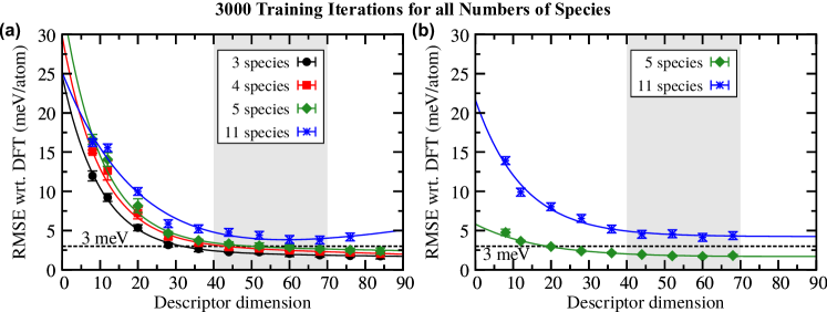
Figure S2: Precision of artificial neural network (ANN) potentials as function of the dimension of the descriptor used to represent the local atomic environment. The root mean squared error (RMSE) after 3,000 training iterations is shown. After this number of iterations, the RMSE has not yet converged for the 11-species systems and is increasing with descriptor size.

The RMSE was evaluated after 3,000 training iterations using the LM-BFGS method Byrd et al. (1995); Zhu et al. (1997), however, with increasing number of species and increasing descriptor size the required number of training iterations to achieve convergence generally also increases. Thus, the ANN potentials for 11 chemical species and descriptor dimensions above 40 have not converged after 3,000 iterations, and the RMSEs after 5,000 iterations are shown in Fig. 1. The unconverged RMSE after 3,000 training iterations is shown in Fig. S2 in the Appendix.

Remarkably, the optimal descriptor dimension is essentially independent of the number of chemical species in the composition, and a descriptor dimension of 44 is sufficient to capture the structural and chemical features of the distinct atomic configurations in the Li$M$O2 data set with up to 11 chemical species.

Figure 1b shows the equivalent analysis for the first-principles energies and structures of 45,892 conformations of the proteinogenic amino acids (5 chemical species: H, C, N, O, and S) and their complexes with the six divalent cations Ba^2+, Ca^2+, Cd^2+, Hg^2+, Pb^2+, Sr^2+ (a total of 11 chemical species) by Ropo, Schneider, Baldauf, and Blum Ropo et al. (2016a) based on DFT calculations (PBE+TS-vdW Tkatchenko and Scheffler (2009)) using the FHI-aims package Blum et al. (2009). This data set was compiled specifically for the parametrization of atomic potentials and thoroughly samples the relevant conformational space Ropo et al. (2016a), an important first step towards improved force fields for proteins Piana et al. (2014). The high precision of the ANN potentials with an RMSE of $\sim$3 meV/atom for 5 and 11 chemical species indicates that our combined descriptor is not limited to crystal structures with similar atomic positions, but is also suitable to distinguish between continuous atomic arrangements.

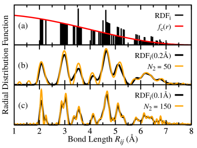
Figure 2: (a) Discrete atom-centered radial distribution function ($\textup{RDF}_{i}$) for a lithium site in a structure with composition Li₂MnNiO₄ (black lines) and the cosine cutoff function $f_{\textup{c}}$ for a cutoff radius of $R_{\textup{c}}=8$ Å. (b) Convolution of the RDF of (a) with a Gaussian function with a width of 0.2 Å (black line) and the reconstructed RDF from a Chebyshev expansion with a radial order $N_{2}=50$ (orange line). (c) Same as (b), but with a Gaussian width of 0.1 Å and an expansion order of $N_{2}=150$.

To understand the significance of these observations, we first describe the details of the structural and compositional descriptor. We begin by expressing the atom-centered radial and angular distribution functions of Eqs. (7) and (2) in terms of discrete delta functions centered at the bond lengths between atoms $j$ and the central atom $i$, $R_{ij}=||\mathbf{R}_{j}-\mathbf{R}_{i}||$, and the bond angle $\theta_{ijk}=\angle(\mathbf{R}_{j}-\mathbf{R}_{i},\mathbf{R}_{k}-\mathbf{R}_{i})$

$$\mathrm{RDF}_{i}(r) =\sum_{\mathclap{\;\;\mathbf{R}_{j}\in\,\sigma_{i}^{R_{\textup{c}}}}}\delta(r-R_{ij})\,f_{\textup{c}}(R_{ij})\,w_{t_{j}}$$ (3)

$$\mathrm{ADF}_{i}(\theta) =\sum_{\mathclap{\;\;\mathbf{R}_{j},\mathbf{R}_{k}\in\,\sigma_{i}^{R_{\textup{c}}}}}\delta(\theta-\theta_{ijk})\,f_{\textup{c}}(R_{ij})\,f_{\textup{c}}(R_{ik})\,w_{t_{j}}w_{t_{k}}\quad,$$ (4)

where $f_{\textup{c}}$ is a cutoff function that smoothly goes to zero at $R_{\textup{c}}$ (in practice, we use $f_{\textup{c}}(r)=0.5[\cos(r\cdot\pi/R_{\textup{c}})+1]$). The weights $w_{t_{j}}$ and $w_{t_{k}}$ are 1 for the structural descriptor ${}^{\{\mathbf{R}\}}\widetilde{\sigma}_{i}^{R_{\textup{c}}}$ and take on species-dependent values for the compositional descriptor ${}^{\{t\}}\widetilde{\sigma}_{i}^{R_{\textup{c}}}$. Here, we followed the (Ising-model) pseudo-spin convention commonly used for lattice models Sanchez et al. (1984), i.e., $w_{l}=0,\pm{}1,\pm{}2,\ldots$ where 0 is omitted for even numbers of species. For the expansions Eqs. (7) and (2) we choose a complete orthonormal basis $\{\phi_{\alpha}\}$, i.e., $\int\phi_{\alpha}\overline{\phi}_{\beta}=1$ if $\alpha=\beta$ and $0$ else. With this choice, the expansion coefficients are given by

$$c^{(2)}_{\alpha} =\sum_{\mathclap{\;\;\mathbf{R}_{j}\in\,\sigma_{i}^{R_{\textup{c}}}}}\phi_{\alpha}(R_{ij})\,f_{\textup{c}}(R_{ij})\,w_{t_{j}}\qquad\text{and}$$ (5)

$$c^{(3)}_{\alpha} =\sum_{\mathclap{\;\;\mathbf{R}_{j},\mathbf{R}_{k}\in\,\sigma_{i}^{R_{\textup{c}}}}}\phi_{\alpha}(\theta_{ijk})\,f_{\textup{c}}(R_{ij})\,f_{\textup{c}}(R_{ik})\,w_{t_{j}}w_{t_{k}}\quad.$$ (6)

A derivation of Eqs. (10) and (6) can be found in the Appendix. The expansions are truncated at finite radial and angular orders $N_{2}$ and $N_{3}$ that determine the dimension (i.e., the complexity) and the resolution of the descriptor, i.e., ${}^{\{\mathbf{R}\}}\widetilde{\sigma}_{i}^{R_{\textup{c}}}=\{{{}^{\{\mathbf{R}\}}c^{(2)}_{1}},\ldots,{{}^{\{\mathbf{R}\}}c^{(2)}_{N_{2}}},{{}^{\{\mathbf{R}\}}c^{(3)}_{1}},\ldots,{{}^{\{\mathbf{R}\}}c^{(3)}_{N_{3}}}\}$.

For this article, we employed the Chebyshev polynomials of the first kind as basis functions (see Appendix), as they can be defined in terms of a recurrence relation that allows for highly efficient numerical evaluation of the function values and their derivatives. With this choice of basis functions, Fig. 2 shows the RDF as reconstructed based on the structural expansion coefficients $\{^{\{\mathbf{R}\}}c_{\alpha}^{(2)}\}$ for two different orders ($N_{2}=50$ and $N_{2}=150$). From comparison with Gaussian convolutions of the discrete RDF, the radial resolution of the expansion order $N_{2}=150$ is around 0.1 Å. Atomic features on smaller scales may affect the shape of the RDF but do not give rise to distinct peaks. The expansion of the ADF is completely analogous.

We note that the radial and angular BP symmetry functions Behler and Parrinello (2007); Behler (2011) can be cast into the form of Eqs. (10) and (6) but are neither orthogonal nor systematically refinable. The relationship of our structural descriptor to the coefficients of a basis set expansion is, in turn, closer in spirit to the SOAP method Bartók et al. (2010, 2013) which is based on the power spectrum of the atomic density of the local atomic environment. SOAP allows for a rigorous and systematic description of the local structure, which comes at the cost of an arithmetically (and computationally) more complex formalism. However, by limiting the descriptor to radial and angular contributions our method maintains the simple analytic nature of the BP approach that allows for a highly efficient numerical implementation and straightforward differentiation (which is required for the calculation of analytic forces and higher derivatives). Basing the radial and angular descriptors on an expansion in a complete basis set allows their systematic refinement in the spirit of the SOAP approach, though our approach is limited to two- and three-body interactions.

Also note that decomposing the local atomic environment into $n$-body contributions as done in our structural descriptor is an established and well-tested approach for lattice models such as the cluster expansion (CE) method Fontaine (1994); Ceder (1993). In CE models, the total configurational energy is expanded in a basis set consisting of site clusters $(s_{i}s_{j}\ldots)$ with increasing numbers of lattice sites $s_{\alpha}$, i.e., point clusters, pairs, trimers, …, $n$-tuples. The site clusters form a complete basis set, and the configurational averages of all equivalent clusters (the cluster correlations) are the descriptor of the CE model. Unlike MLPs, the CE energy is a linear function of the descriptor. For the case of the continuous structural energy, Thompson et al. demonstrated that a linear potential based on SOAP (which also is a complete basis of the local structure) can achieve reasonable accuracy in practice if a sufficient number of basis functions is used Thompson et al. (2014).

However, the strength of non-linear machine-learning models is that they do not require mathematically complete descriptors as long as the descriptor is able to differentiate between all relevant samples. This property is exploited, for example, in the area of image recognition and text classification Rogati and Yang (2002). In practice this means that even an incomplete descriptor of the local atomic environment may be sufficient to construct a non-linear MLP if that descriptor is able to differentiate between all relevant local atomic structures, i.e., the descriptor does not have to resolve all hypothetically possible sets of three dimensional coordinates.

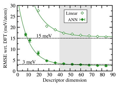
Figure 3: Convergence of the root mean squared error (RMSE) of the predicted Li$M$O2 (5 species, $M$ = Ti, Mn, Ni) energy for a linear model (empty diamonds) and a non-linear ANN (filled diamonds) with the dimension of the combined descriptor. The gray region highlights descriptors that result in essentially converged ANN potentials with RMSE values around 3 meV/atom. The lines are meant to guide the eye.

This behavior is exemplified in Fig. 3, which compares the precision of an ANN potential for the Li$M$O2 data set with 5 chemical species (10,175 atomic configurations) with that of a linear energy model as function of the descriptor dimension. As seen in the figure, the ANN achieves an RMSE of $\leq$3 meV/atom with descriptor dimensions of 44 (22 basis functions) and larger. Comparison with Fig. 2 shows that such a small basis set corresponds to a coarse representation of the RDF and the ADF, however, obviously this level of approximation is sufficient for the ANN potential to differentiate between all structural and compositional features in the reference set. This is not the case for the linear model whose RMSE is $>$15 meV/atom even for a descriptor dimension of 84.

In conclusion, we showed that machine-learning potentials do not require (mathematically) complete descriptors of the local atomic environment to reproduce potential energy surfaces with high precision. With this insight, we devised a combined descriptor of the local atomic structure and composition whose complexity does not scale with the number of chemical species. The method is conceptually simple and allows for highly efficient numerical implementations. The utility of the approach was demonstrated for two exemplary materials classes, lithium transition-metal oxides and amino acid complexes, each separately comprising compositions with 11 different chemical species. We showed that the potential energy landscape of both example systems can be represented with high precision by artificial neural network potentials using the combined descriptor achieving a resolution of around 3 meV/atom. Hence, machine-learning potentials are in practice not limited to compositions with small numbers of chemical species as previously argued in the literature and may be effective for the modeling of high-dimensional materials such as oxide solid solutions and peptide chains.

I Acknowledgments

This work was supported by the Office of Naval Research (ONR) under ONR award N00014-14-1-0444. This work used mainly the computational facilities of the Extreme Science and Engineering Discovery Environment (XSEDE), which is supported by National Science Foundation grant no. ACI-1053575. Additional computational resources from the University of California Berkeley, HPC Cluster (SAVIO) are also gratefully acknowledged.

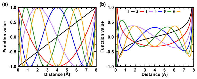
Figure S1: (a) Dual basis functions of Eq. (14) (Chebyshev polynomials) up to order $\alpha=6$ for a catoff radius $R_{\textup{c}}=8.0$ Å. The polynomial of order $\alpha=0$ is constant 1 and not shown. (b) The corresponding basis functions of Eq. (13) (only needed for the reconstruction of the RDF or ADF).

Appendix A The $\textup{Li}M\textup{O}_{2}$ data set

Starting point for the generation of the Li$M$O2 data set of this work were the enumerated lithium transition-metal (TM) oxide configurations of reference Urban et al., 2016. The data set with 3 chemical species (Li, Ti, and O) comprised a total of 7,338 structures including the TiO2 structures from reference Artrith and Urban, 2016 and additional LiTiO2 configurations that were systematically enumerated based on the rocksalt structure (A sites = Li and Ti, B sites = O) up to cell sizes containing 8 cation sites using the approach by Hart et al. Hart and Forcade (2008, 2009); Hart et al. (2012). For the data set with 4 chemical species (Li, Ni, Ti, and O), 1,343 atomic configurations with compositions LiNiO2 and Li2NiTiO4 were additionally generated using the same enumeration methodology (giving a total of 8,681 configurations). Further, 1,494 atomic configurations with compositions LiMnO2 and Li2NiMnO4 were added for the set with 5 species (Li, Ti, Mn, Ni, O) to a total of 10,175 configurations. Finally, for 11 chemical species, random atomic configurations with composition Li9$M$9O18 with $M$ = Sc, Ti, V, Cr, Mn, Fe, Co, Ni, Cu for all 24,310 possible compositions were generated, and 5,872 randomly selected configurations were included in the reference data set.

The complete reference data set for 11 chemical species comprises a total of 16,047 atomic configurations.

Appendix B Artificial neural network potentials

Together with the dimension of the descriptor discussed in the main text, the architecture of an artificial neural network (ANN) determines the model complexity. For the feedforward ANNs used in the present work, the architecture is given by the number of hidden layers and the number of nodes per layer employed by the ANN (see also reference Artrith and Urban (2016) for a detailed introduction). To facilitate comparison of the different structure and composition spaces on equal footing, we generally used a $N$-15-15-1 ANN architecture, i.e., an architecture with two hidden layeres containing each 15 nodes independent of the descriptor dimension $N$.

The atomic energy network (aenet) software Artrith and Urban (2016) was employed for the training of the ANN potentials with the limited-memory BFGS method Byrd et al. (1995); Zhu et al. (1997).

Appendix C Scaling behavior of existing local descriptors

The complexity of the Behler–Parrinello (BP) descriptor and the cluster-expansion basis scales at least quadratically with the number of chemical species.

As noted in the main manuscript, separate MLPs for each chemical species are constructed. For each of these MLPs, the descriptor also scales with the number of species:

For example, the angular symmetry functions for an ANN potential for a single species A describe the interactions of the central atom with two atoms of type A (A-A). For two species A and B, three interactions occur (A-A, A-B, and B-B), and for three species A, B, C, there are six (A-A, A-B, A-C, B-B, B-C, C-C). In general, for $N$ species the number of interactions is $N(N+1)/2$, i.e., the scaling is quadratic in the number of species. Further details about the symmetry function set up for multicomponent systems using the Behler-Parrinello approach along with actual parameters can also be found in reference Artrith et al., 2013.

When Ising-like pseudo spin variables are used to describe compositions, as for example in the cluster expansion (CE) method, an analogous scaling with the number of species occurs. The number of CE basis functions scales quadractically with the number of species when only pair clusters are considered. Generally, the scaling is on the order of the highest included n-body interaction, i.e., cubic for triplets, 4th order for quadruplet interactions, and so on. Mathematically, this relationship was worked out in reference Sanchez et al., 1984.

The multi-component implementation of the smooth overlap of atomic positions (SOAP) approach, is laid out in section 2.3 of reference De et al., 2016. The scaling is also quadratic, as it involves partial power spectra for each pair of species.

Appendix D Derivation of the expansion coefficients

The expansion coefficient $c^{(2)}_{\alpha}$ of the basis set expansion of the radial distribution function (RDF)

$$\mathrm{RDF}_{i}(r)=\sum_{\alpha}c^{(2)}_{\alpha}\phi_{\alpha}(r)\quad,$$ (7)

where $\int\bar{\phi}_{\beta}(r)\phi_{\alpha}(r)\,\mathrm{d}r=\delta_{\beta\alpha}$ and $\{\bar{\phi}_{\alpha}\}$ is the orthogonal dual basis to $\{\phi_{\alpha}\}$, is given by

$$c^{(2)}_{\alpha}=\!\int_{0}^{R_{\textup{c}}}\!\bar{\phi}_{\alpha}(r)\,\mathrm{RDF}_{i}(r)\,\mathrm{d}r\quad.$$ (8)

Note that the RDF as defined in Eq. (4) of the main manuscript

$$\mathrm{RDF}_{i}(r) =\sum_{\mathclap{\;\;\mathbf{R}_{j}\in\,\sigma_{i}^{R_{\textup{c}}}}}\delta(r-R_{ij})\,f_{\textup{c}}(R_{ij})\,w_{t_{j}}$$ (9)

is only different from $0$ for $0\leq{}r\leq{}R_{\textup{c}}$, so that the integral in Eq. (8) can be replaced by an integral over the entire space. Inserting the expression of the RDF Eq. (9) into the Eq. (8) yields

$$c^{(2)}_{\alpha} =\sum_{\mathclap{\;\;\mathbf{R}_{j}\in\,\sigma_{i}^{R_{\textup{c}}}}}\quad\int\!\bar{\phi}_{\alpha}(r)\,\delta(r-R_{ij})\,f_{\textup{c}}(R_{ij})\,w_{t_{j}}\,\mathrm{d}r$$

$$=\sum_{\mathclap{\;\;\mathbf{R}_{j}\in\,\sigma_{i}^{R_{\textup{c}}}}}\bar{\phi}_{\alpha}(R_{ij})\,f_{\textup{c}}(R_{ij})\,w_{t_{j}}\quad,$$ (10)

which is the expression given in Eq. (6) of the main manuscript.

The derivation of the coefficients $c^{(3)}_{\alpha}$ of the angular expansion is completely analogous.

Appendix E Chebyshev polynomials of the first kind

The Chebyshev polynomials $\{T_{n}\}$ are defined by the recurrence relation

$$\begin{aligned} T_{0}(x)&=1\\ T_{1}(x)&=x\\ T_{n+1}(x)&=2xT_{n}(x)-T_{n-1}(x)\quad.\end{aligned}$$ (11)

The polynomials are orthogonal on the interval $[-1,1]$ with respect to a weight

$$\int_{-1}^{1}\!\!\!T_{n}(x)T_{m}(x)\frac{\mathrm{d}x}{\sqrt{1-x^{2}}}=\begin{cases}\pi&n=m=0\\ \frac{\pi}{2}&n=m\neq{}0\\ 0&\text{else}\end{cases}$$ (12)

so that we choose the basis functions $\{\phi_{\alpha}\}$ and their duals $\{\bar{\phi}_{\alpha}\}$ on the interval $r\in{}(0,R_{\textup{c}})$ (for the radial expansion) as

$$\phi_{\alpha}(r) =\frac{k}{2\pi\sqrt{\frac{r}{R_{\textup{c}}}-\frac{r^{2}}{R^{2}_{\textup{c}}}}}\,T_{\alpha}\Bigl{(}\frac{2r}{R_{\textup{c}}}-1\Bigr{)}$$ (13)

$$\text{and}\quad\bar{\phi}_{\alpha}(r) =T_{\alpha}\Bigl{(}\frac{2r}{R_{\textup{c}}}-1\Bigr{)}\quad\text{with}\quad 0<r<R_{\textup{c}}$$ (14)

where $k=1/2$ for $\alpha=0$ and $k=1$ otherwise. For the angular expansion, the appropriate interval is $0\leq{}\theta<\pi$, so that $R_{\textup{c}}$ has to be replaced by $\pi$ in Eqs. (13) and (14).

References

- Lorenz et al. (2004) S. Lorenz, A. Groß, and M. Scheffler, Chem. Phys. Lett. 395, 210 (2004).
- Behler and Parrinello (2007) J. Behler and M. Parrinello, Phys. Rev. Lett. 98, 146401 (2007).
- Bartók et al. (2010) A. P. Bartók, M. C. Payne, R. Kondor, and G. Csányi, Phys. Rev. Lett. 104, 136403 (2010).
- Rupp et al. (2012) M. Rupp, A. Tkatchenko, K.-R. Müller, and O. A. von Lilienfeld, Phys. Rev. Lett. 108, 058301 (2012).
- Montavon et al. (2012) G. Montavon, G. B. Orr, and K.-R. Müller, eds., Neural Networks: Tricks of the Trade (Second Edition), Lecture Notes in Computer Science, Vol. 7700 (Springer Berlin Heidelberg, 2012).
- Rasmussen and Williams (2006) C. E. Rasmussen and C. K. I. Williams, Gaussian Processes for Machine Learning (MIT University Press Group Ltd, 2006).
- Artrith et al. (2011) N. Artrith, T. Morawietz, and J. Behler, Phys. Rev. B 83, 153101 (2011).
- Artrith and Kolpak (2014) N. Artrith and A. M. Kolpak, Nano Lett. 14, 2670– (2014).
- Artrith and Kolpak (2015) N. Artrith and A. M. Kolpak, Comput. Mater. Sci. 110, 20–28 (2015).
- Morawietz et al. (2016) T. Morawietz, A. Singraber, C. Dellago, and J. Behler, Proc. Natl. Acad. Sci. USA 113, 8368 (2016).
- Faber et al. (2016) F. A. Faber, A. Lindmaa, O. A. von Lilienfeld, and R. Armiento, Phys. Rev. Lett. 117, 135502 (2016).
- Huo and Rupp (2017) H. Huo and M. Rupp, arXiv (2017), 1704.06439 .
- De et al. (2016) S. De, A. P. Bartok, G. Csanyi, and M. Ceriotti, Phys. Chem. Chem. Phys. 18, 13754 (2016).
- Lee et al. (2014) J. Lee, A. Urban, X. Li, D. Su, G. Hautier, and G. Ceder, Science 343, 519 (2014).
- Yabuuchi et al. (2015) N. Yabuuchi, M. Takeuchi, M. Nakayama, H. Shiiba, M. Ogawa, K. Nakayama, T. Ohta, D. Endo, T. Ozaki, T. Inamasu, K. Sato, and S. Komaba, Proc. Natl. Acad. Sci. USA 112, 7650–7655 (2015).
- Ropo et al. (2016a) M. Ropo, M. Schneider, C. Baldauf, and V. Blum, Sci. Data 3, 160009 (2016a).
- Ropo et al. (2016b) M. Ropo, V. Blum, and C. Baldauf, Sci. Rep. 6, 35772 (2016b).
- Daw and Baskes (1984) M. S. Daw and M. I. Baskes, Phys. Rev. B 29, 6443 (1984).
- Daw et al. (1993) M. S. Daw, S. M. Foiles, and M. I. Baskes, Mater. Sci. Rep. 9, 251 (1993).
- Behler (2011) J. Behler, J. Chem. Phys. 134, 074106 (2011).
- Bartók et al. (2013) A. P. Bartók, R. Kondor, and G. Csányi, Phys. Rev. B 87, 184115 (2013).
- Sadeghi et al. (2013) A. Sadeghi, S. A. Ghasemi, B. Schaefer, S. Mohr, M. A. Lill, and S. Goedecker, J. Chem. Phys. 139, 184118 (2013).
- Schütt et al. (2014) K. T. Schütt, H. Glawe, F. Brockherde, A. Sanna, K. R. Müller, and E. K. U. Gross, Phys. Rev. B 89, 205118 (2014).
- Behler (2015) J. Behler, Int. J. Quantum Chem. 115, 1032 (2015).
- Faber et al. (2015) F. Faber, A. Lindmaa, O. A. von Lilienfeld, and R. Armiento, Int. J. Quantum Chem. 115, 1094 (2015).
- von Lilienfeld et al. (2015) O. A. von Lilienfeld, R. Ramakrishnan, M. Rupp, and A. Knoll, Int. J. Quantum Chem. 115, 1084 (2015).
- Bartók and Csányi (2015) A. P. Bartók and G. Csányi, Int. J. Quantum Chem. 115, 1051 (2015).
- Artrith and Urban (2016) N. Artrith and A. Urban, Comput. Mater. Sci. 114, 135 (2016).
- Hornik (1991) K. Hornik, Neural Networks 4, 251 (1991).
- Liechtenstein et al. (1995) A. I. Liechtenstein, V. I. Anisimov, and J. Zaanen, Phys. Rev. B 52, R5467 (1995).
- Anisimov et al. (1997) V. I. Anisimov, F. Aryasetiawan, and A. I. Lichtenstein, J. Phys.: Condens. Matter 9, 767 (1997).
- Jain et al. (2011) A. Jain, G. Hautier, C. J. Moore, S. P. Ong, C. C. Fischer, T. Mueller, K. A. Persson, and G. Ceder, Comput. Mater. Sci. 50, 2295 (2011).
- Perdew et al. (1996) J. Perdew, K. Burke, and M. Ernzerhof, Phys. Rev. Lett. 77, 3865 (1996).
- Blöchl (1994) P. E. Blöchl, Phys. Rev. B 50, 17953 (1994).
- Kresse and Furthmüller (1996a) G. Kresse and J. Furthmüller, Phys. Rev. B 54, 11169 (1996a).
- Kresse and Furthmüller (1996b) G. Kresse and J. Furthmüller, Comput. Mater. Sci. 6, 15 (1996b).
- Ong et al. (2013) S. P. Ong, W. D. Richards, A. Jain, G. Hautier, M. Kocher, S. Cholia, D. Gunter, V. L. Chevrier, K. A. Persson, and G. Ceder, Comput. Mater. Sci. 68, 314 (2013).
- Byrd et al. (1995) R. Byrd, P. Lu, J. Nocedal, and C. Zhu, SIAM J. Sci. Comput. 16, 1190 (1995).
- Zhu et al. (1997) C. Zhu, R. H. Byrd, P. Lu, and J. Nocedal, ACM T. Math Software 23, 550–560 (1997).
- Tkatchenko and Scheffler (2009) A. Tkatchenko and M. Scheffler, Phys. Rev. Lett. 102, 073005 (2009).
- Blum et al. (2009) V. Blum, R. Gehrke, F. Hanke, P. Havu, V. Havu, X. Ren, K. Reuter, and M. Scheffler, Comput. Phys. Commun. 180, 2175 (2009).
- Piana et al. (2014) S. Piana, J. L. Klepeis, and D. E. Shaw, Curr. Opin. Struct. Biol. 24, 98 (2014).
- Sanchez et al. (1984) J. Sanchez, F. Ducastelle, and D. Gratias, Physica A 128, 334 (1984).
- Fontaine (1994) D. D. Fontaine, Solid State Phys. 47, 33–176 (1994).
- Ceder (1993) G. Ceder, Comput. Mater. Sci. 1, 144 (1993).
- Thompson et al. (2014) A. Thompson, L. Swiler, C. Trott, S. Foiles, and G. Tucker, J. Comput. Phys. 285, 316 (2014).
- Rogati and Yang (2002) M. Rogati and Y. Yang, in Proceedings of the eleventh international conference on Information and knowledge management - CIKM ’02 (ACM Press, 2002).
- Urban et al. (2016) A. Urban, I. Matts, A. Abdellahi, and G. Ceder, Adv. Energy Mater. 6, 1600488 (2016).
- Hart and Forcade (2008) G. L. W. Hart and R. W. Forcade, Phys. Rev. B 77, 224115 (2008).
- Hart and Forcade (2009) G. L. W. Hart and R. W. Forcade, Phys. Rev. B 80, 014120 (2009).
- Hart et al. (2012) G. L. Hart, L. J. Nelson, and R. W. Forcade, Comput. Mater. Sci. 59, 101 (2012).
- Artrith et al. (2013) N. Artrith, B. Hiller, and J. Behler, physica status solidi (b) 250, 1191 (2013).