A review and comparative study on functional time series techniques

Summary

This paper reviews the main estimation and prediction results derived in the context of functional time series, when Hilbert and Banach spaces are considered, specially, in the context of autoregressive processes of order one (ARH(1) and ARB(1) processes, for $H$ and $B$ being a Hilbert and Banach space, respectively). Particularly, we pay attention to the estimation and prediction results, and statistical tests, derived in both parametric and non-parametric frameworks. A comparative study between different ARH(1) prediction approaches is developed in the simulation study undertaken.

Key words: ARH processes; Banach spaces; comparative study; empirical eigenvectors; functional linear regression; functional time series; Hilbert spaces; Hilbert-Schmidt autocorrelation operator; strongly-consistent estimator; trace covariance operators.

1 Introduction

Since the beginning, time series analysis has played a key role in the analysis of temporal correlated data. Due to the huge computing advances, data began to be gathered with an increasingly temporal resolution level. Statistical analysis of temporal correlated high-dimensional data has then become a very active research area. This paper presents an overview of the main estimation and prediction approaches, formulated in the context of functional time series.

Autoregressive Hilbertian processes of order one (ARH(1) processes) were firstly introduced by Bosq (1991), where a real separable Hilbert space $H$ is considered. The functional estimation problem was addressed by a moment-based estimation of the linear bounded autocorrelation operator, involved in the conditional expectation, providing the least-squares functional predictor (ARH(1) predictor). Projection into the theoretical and empirical eigenvectors of the autocovariance operator is considered in the computation of a consistent moment-based estimator of the autocorrelation operator. The model introduced in Bosq (1991) has been successfully used by Cavallini et al. (1994), on the forecasting of electricity consumption in Bologna (Italy). Central limit theorems, formulated in Merlevède (1996) and Merlevède et al. (1997), were applied to derive the asymptotic properties of ARH(1) parameter estimators and predictors (see, e.g., Bosq, 1999a, 1999b). Close graph Theorem allowed Mas (1999) to derive a truncated componentwise estimator of the adjoint of the autocorrelation operator. A central limit theorem for the formulated estimator was also derived. Enhancements to the model firstly established in Bosq (1991), under the Hilbert-Schmidt assumption of the autocorrelation operator, were presented in the comprehensive monograph by Bosq (2000). Specifically, the asymptotic properties of the formulated truncated componentwise parameter estimator of the autocorrelation operator, and of their associated plug-in predictors, are derived, from the asymptotic behaviour of the empirical eigenvalues and eigenvectors of the autocovariance operator. Improvements of the above-referred results were also provided in Mas (2000), where an extra regularity condition on the inverse of the autocovariance operator was imposed, to obtain the so-called resolvent class estimators. Efficiency of the componentwise estimator of the autocorrelation operator proposed in Bosq (2000) was studied in Guillas (2001). Mas & Menneateau (2003a) proved some extra asymptotic results for the empirical functional second-order moments. Mas & Menneateau (2003b) applied the perturbation theory, in the derivation of the asymptotic properties of the proposed estimators. Asymptotic behaviour of the ARH(1) estimators was obtained in Mas (2004, 2007) under weaker assumptions (in particular, under the assumption of compactness of the autocorrelation operator). Menneateau (2005) formulated some laws of the iterated logarithm for an ARH(1) process. Weak-consistency results, in the norm of Hilbert-Schmidt operators, have been recently proposed in Álvarez-Liébana et al. (2017), when the covariance and autocorrelation operators admit a diagonal spectral decomposition, in terms of a common eigenvectors system, under the Hilbert-Schmidt assumption of the autocorrelation operator. Alternative ARH(1) estimation techniques are presented in Besse & Cardot (1996), where a spline-smoothed-penalized functional principal component analysis (spline-smoothed-penalized FPCA), with rank constraint, was performed. A spline-smoothed-penalized FPCA estimator of the autocorrelation operator of an ARH(p) process was obtained in Cardot (1998), proving its consistency. A robust spline-smoothed-penalized FPCA estimator of the autocorrelation operator, for a class of ARH(1) processes, was discussed in Besse et al. (2000).

Statistical tests for the lack of dependence, in the context of linear processes in function spaces, were derived in Kokoszka et al. (2008). Change point analysis was applied to test the stability and stationarity of an ARH(1) process, in Horváth et al. (2010) and Horváth et al. (2014), respectively. A practical survey about how the ARH(1) framework can be applied to forecasting electricity consumption was presented in Andersson & Lillestøl (2010). The asymptotic normality of the empirical autocovariance operator, and its associated eigenelements, was studied in Kokoszka & Reimherr (2013a), in the context of non-linear and weakly dependent functional time series. Consistency results of componentwise parameter estimators addressed in Hörmann & Kidziński (2015), in the context of a general functional linear regression, can be particularized to the ARH(1) framework, under weaker assumptions than those ones assumed in Bosq (2000). The case of the autocorrelation operator depending on an unknown real-valued parameter has been also considered (see Kara-Terki & Mourid, 2016). This scenario can be applied to the prediction of an Ornstein-Uhlenbeck process in the ARH(1) framework, as developed in Álvarez-Liébana et al. (2016).

An extension of the classical ARH(1) to ARH(p) processes, with $p$ greater than one, was established in Bosq (2000). The crucial choice of the lag order $p$ was discussed in Kokoszka & Reimherr (2013b). An extended class of ARH(1) processes, by including exogenous variables in their dependence structure, was formulated in Guillas (2000). An ARH(p) model, with $p$ greater than one, to modelling the exogenous random variables, was subsequently proposed by Damon & Guillas (2002). Indeed, Damon & Guillas (2005) derived a Markovian representation by its reformulation as a $H^{p}$-valued ARHX(1) process. Marion & Pumo (2004) considered the first derivatives of an ARH(1) process, as the exogenous variables to be included in the model, by introducing the so-called ARHD(1) process. The ARHD(1) process was characterized as a particular ARH(1) model in Mas & Pumo (2007). Conditional autoregressive Hilbertian processes of order one (CARH(1) processes, also known as doubly stochastic Hilbertian process of order one), were introduced in Guillas (2002), aimed to include exogenous information in a non-additive way (see also Cugliary, 2013, where an underlying multivariate process was considered). Mourid (2004) considers the randomness of the autocorrelation operator by conditioning to each element of the sample space. ARH(p) processes with random coefficients (RARH(p) processes) were then defined. Some asymptotic results for the already mentioned RARH(p) processes are provided in Allam & Mourid (2014). Weakly dependent processes were analysed in Hörmann & Kokoszka (2010). Hilbertian periodically correlated autoregressive processes of order one (PCARH(1) processes) have been defined by Soltani & Hashemi (2011), and later extended to the Banach-valued context by Parvardeh et al. (2017). Spatial extension of the classical ARH(1) models was firstly proposed in Ruiz-Medina (2011). Their moment-based estimation was detailed in Ruiz-Medina (2012). An extension, to the context of processes in function spaces, of the well-known real-valued ARCH model, has been derived in Hörmann et al. (2013). Recently, Ruiz-Medina & Álvarez-Liébana (2017a) derived the asymptotic efficiency and equivalence of both, classical and Beta-prior-based Bayesian diagonal componentwise ARH(1) parameter estimators and predictors, when the autocorrelation operator is not assumed to be a compact operator, in the Gaussian case. Ruiz-Medina & Álvarez-Liébana (2017b) provide sufficient conditions for the strong-consistency, in the trace norm, of the autocorrelation operator of an ARH(1) process, when it does not admit a diagonal spectral decomposition in terms of the eigenvectors of the autocovariance operator. A two-level hierarchical Gaussian model is applied in Kowal et al. (2017) on the forecasting of ARH(p) processes.

Concerning alternative bases, Grenander’s theory of sieves (see Grenander, 1981) was adapted by Bensmain & Mourid (2001), for the estimation of the autocorrelation operator of an ARH(1) process, from a Fourier-basis-based decomposition in a finite dimensional subspace. An integral form of the autocorrelation operator was assumed in Laukaitis & Rac̆kauskas (2002), who consider smoothing techniques based on B-spline and Fourier bases. Antoniadis & Sapatinas (2003) suggested three linear wavelet-based predictors, two of them are built from the componentwise and resolvent estimators of the autocorrelation operator, already established in Bosq (2000) and Mas (2000), respectively. Hyndman & Ullah (2007) formulated a prediction approach of the mortality and fertility rates based on a real-valued ARIMA forecasting of the FPC scores, for each non-parametric smoothed sample curve. Focusing on the predictor, the idea of replacing the FPC with the directions more relevant to forecasting, by searching a reduced-rank approximation, was firstly exhibited in Kargin & Onatski (2008) (see also Didericksen et al., 2012, where approaches by Bosq, 2000, and Kargin & Onatski, 2008, were compared). As an extension of the work by Hyndman & Ullah (2007), a weighted version of the FPLSR and FPCA approaches was established in Hyndman & Shang (2009), with a decreasing weighting over time, as often, e.g., in demography. For the purpose of taking into account the information coming from the dynamic dependence, which is usually ignored in the FPCA literature, a dynamic functional principal components approach was simultaneously introduced by Panaretos & Tavakoli (2013) and Hörman et al. (2015). The main difference between them lies in the explicit construction of the dynamic scores performed in Hörman et al. (2015), while a functional process of finite rank was built in Panaretos & Tavakoli (2013). As discussed in Aue et al. (2015), a multivariate VARMA approach can be used to improve the curve-by-curve approaches above-referred by Hyndman & Ullah (2007) and Hyndman & Shang (2009).

Moving-average Hilbertian processes (MAH processes) and ARMAH processes can be defined as a particular case of Hilbertian general linear processes (LPH). From the previous above-referred works by Bosq (1991) and Mourid (1993), sufficient conditions for the invertibility of LPH were provided in Merlevède (1995, 1996). A Markovian representation of a stationary and invertible LPH, as well as a consistent plug-in predictor, was derived in Merlevède (1997). A few new asymptotic results were derived by Bosq (2000) from the previous theoretical properties. The conditional central limit theorem (see Dedecker & Merlevède, 2002) was extended to functional stochastic processes in Dedecker & Merlevède (2003), allowing its application to LPH. The weak convergence for the empirical autocovariance and cross-covariance operators of LPH was proved in Mas (2002). Further results, that those one formulated in Bosq (2000) for LPH, were obtained by Bosq (2007) and Bosq & Blanke (2007), where the study of a consistent predictor of MAH processes was addressed. Componentwise estimation of a MAH(1) process was studied in Turbillon et al. (2008), under properly assumptions. Tools proposed in Hyndman & Shang (2008) can be used in the outlier detection of an observed ARMAH(p,q) process. Wang (2008) proposed a real-valued non-linear ARMA model in which functional MA coefficients were considered (see also Chen et al., 2016, where MA coefficients were given by smooth functions). Tensorial products of ARMAH processes have been analysed in Bosq (2010), when innovations are assumed to be a martingale differences sequence.

An extensive literature has been also developed concerning the Banach-valued time series framework. Strong-consistency results on the estimation of a Banach-valued autoregressive process of order one (ARB(1) process) were presented in Pumo (1992, 1998), when $B=\mathcal{C}([0,1]))$ (so-called $AR\mathcal{C}(1)$ process). Its natural extension to $AR\mathcal{C}(p)$ models, with $p$ greater than one, and the characterization of the Ornstein-Uhlenbeck process as an $AR\mathcal{C}(1)$ process, was addressed in Mourid (1993, 1996), respectively. The notion of non-causality was developed in Guillas (2000) for Banach-valued stochastic processes, while the suitable periodicity of the ARB representation was determined by Benyelles & Mourid (2001). Kuelb’s Lemma (see Kuelbs, 1976) played a key role in this Banach-valued framework, since it provides a dense and continuous embedding $B\hookrightarrow H$, where $H$ is the completation of $B$ under a weaker topology (see Labbas & Mourid, 2002, where a componentwise estimation of the autocorrelation operator of an ARB(1) process is achieved in a general real separable Banach space). Non-plug-in $AR\mathcal{C}(1)$ prediction is achieved in Mokhtari & Mourid (2003), applying the theory of Reproducing Kernel Hilbert Spaces (RKHSs). Dehling & Sharipov (2005) addressed the asymptotic properties of both empirical mean and empirical autocovariance operator, for an ARB process with weakly dependent innovation process. A wide monograph concerning the estimation of ARB processes, by using the already mentioned sieve estimators, was developed by Rachedi (2005). Recently, for $\mathcal{D}=\mathcal{D}([0,1])$ space (the space of right-continuous functions with left limits), El Hajj (2011, 2013) have derived the asymptotic properties of the parameter estimators and predictors of $AR\mathcal{D}(1)$ processes. The intensity of jumps for these $\mathcal{D}$-valued processes was later analysed in Blanke & Bosq (2014). Stationarity of ARMAB processes was studied in Spangenberg (2013), under suitable conditions. Central limit theorems for PCARB(1) processes have been recently derived in Parvardeh et al. (2017).

A great amount of authors have been developed alternative non-parametric prediction techniques in both functional time series and functional regression frameworks, where the main goal is to forecast the predictable part of the paths by applying non-parametric methods. Besse et al. (2000) formulated a functional non-parametric kernel-based predictor of an ARH(1) process. Their work can be seen as a functional extension of the methodology adopted in Poggi (1994), where a non-parametric kernel-based forecasting of the electricity consumption was performed in a multivariate framework. Non-parametric methods were proposed in Cuevas et al. (2002), in the estimation of the underlying linear operator of a functional linear regression, where both explanatory and response variables are valued in a function space. A two-steps prediction approach, based on a non-parametric kernel-based prediction of the scaling coefficients, with respect to a wavelet basis decomposition of a stationary stochastic process with values in a function space, was firstly exhibited in Antoniadis et al. (2006). This method, also so-called kernel wavelet functional (KWF) method, was used, and slightly modified, in Antoniadis et al. (2012), on the forecasting of French electricity consumption, when the hypothesis of stationarity is not held. Improvements in the KWF approach were suggested in Cugliari (2011), where continuous wavelet transforms are also considered. A functional version of principal component regression (FPCR), and partial least-squares regression (FPLSR), was formulated by Reiss & Ogden (2007). In the case where the response is a Hilbert-valued variable, and the explanatory variable takes its values in a general function space, equipped with a semi-metric, Ferraty et al. (2012) obtained a non-parametric kernel estimator of the underlying regression operator.

The outline of this paper is as follows. References detailed in Sections 2-7 are divided by thematic areas in a chronicle. Section 2 is devoted to the study of the different ARH(1) componentwise estimation frameworks, as well as related results, based on the projections into the theoretical and empirical eigenvectors of the autocovariance operator. Section 3 deals improvements of the classical ARH(1) framework. Parametric forecasting of functional time series, based on the projection into alternative bases, such as Fourier, B-spline or wavelet bases, will be presented in Section 4. Section 5 studies MAH processes, as a particular case of LPH. The Banach-valued context is detailed in Section 6. Non-parametric techniques, in the context of functional time series and functional linear regression, are described in Section 7. Section 8 will introduce the main elements involved in the particular context of the ARH(1) diagonal componentwise estimation. In Section 9, a comparative study is undertaken for illustration of the performance of some of the most used estimation and prediction ARH(1) methodologies. Specifically, the approaches presented in Álvarez-Liébana et al. (2017), Antoniadis & Sapatinas (2003), Besse et al. (2000), Bosq (2000) and Guillas (2001) are compared. Proof details and useful theoretical results are provided in the Supplementary Material (see Sections S.1-S.3), where the numerical results obtained in the simulation and comparative studies are outlined as well (see Sections S.4-S.5).

2 ARH(1) componentwise estimator, based on the eigenvectors of the autocovariance operator

ARH(1) processes introduced by Bosq (1991) seek to extend the classical AR(1) model to functional data. In that work, a continuous-time stochastic process $\xi=\left\{\xi_{t},\ t\geq 0\right\}$ is turned into a set of $H$-valued random variables $X=\left\{X_{n}(t)=\xi_{n\delta+t},\ n\in\mathbb{Z}\right\}$, with $0\leq t\leq\delta$. In the sequel, let us consider zero-mean stationary processes, being $H$ a real separable Hilbert. The ARH(1) process was defined by

$$X_{n}=\rho\left(X_{n-1}\right)+\varepsilon_{n},\quad X_{n},\leavevmode\nobreak\ \varepsilon_{n}\in H,\quad n\in\mathbb{Z},\quad\rho\in\mathcal{L}(H),$$ (1)

where $\mathcal{L}(H)$ is the space of bounded linear operators on $H$. If $\varepsilon=\left\{\varepsilon_{n},\ n\in\mathbb{Z}\right\}$ is assumed to be a $H$-valued strong white noise (and uncorrelated with $X_{0}$), $\displaystyle\sum_{j=0}^{\infty}\left\|\rho^{j}\right\|_{\mathcal{L}(H)}^{2}<\infty$ is required to the stationarity condition. From the central limit theorems formulated in Merlevède (1996) and Merlevède et al. (1997), the following asymptotic results for the autocovariance operator $C={\rm E}\left\{X_{n}\otimes X_{n}\right\}$, for $n\in\mathbb{Z}$, under ${\rm E}\left\{\left\|X_{0}\right\|_{H}^{4}\right\}<\infty$ (so-called Assumption A3) and $\left\|X_{0}\right\|_{H}<\infty$, were obtained in Bosq (1999a, 1999b):

$$Z_{i}=X_{i}\otimes X_{i}-C=R\left(Z_{i-1}\right)+E_{i},\quad R(z)=\rho z\rho^{*}\in\mathcal{S}(H),\quad\left\|C_{n}-C\right\|_{\mathcal{S}(H)}=\mathcal{O}\left(\left(\frac{\ln(n)}{n}\right)^{1/2}\right)\leavevmode\nobreak\ a.s.,$$ (2)

being $C_{n}=\frac{1}{n}\displaystyle\sum_{i=0}^{n-1}X_{i}\otimes X_{i}$, for each $n\geq 2$, $\left\{E_{n},\ n\in\mathbb{Z}\right\}$ a martingale difference sequence and $\mathcal{S}(H)$ the class of Hilbert-Schmidt operators on $H$. Since $C$ is compact, from the close graph Theorem, $\rho^{*}=C^{-1}D$ is bounded of the domain of $C^{-1}$, which is a dense subspace in $H$. Then, the autocorrelation operator can be built as $\rho=Ext\left(DC^{-1}\right)=\left(DC^{-1}\right)^{**}$. Mas (1999) provided the asymptotic normality of the formulated estimator of $\rho^{*}$, under ${\rm E}\left\{\left\|C^{-1}\varepsilon_{0}\right\|_{H}^{2}\right\}<\infty$, by projecting into $H_{k_{n}}=sp\left(\phi_{1},\ldots,\phi_{k_{n}}\right)$, when the eigenvectors $\left\{\phi_{j},\ j\geq 1\right\}$ of $C$ are assumed to be known. Assumption $C_{1}>\ldots>C_{j}>\ldots>0$ (Assumption A1) was also imposed, where $\left\{C_{j},\ j\geq 1\right\}$ denote the eigenvalues of $C$.

The asymptotic results formulated in Merlevède (1996) and Merlevède et al. (1997) are crucial in the derivation of some extra asymptotic properties for $C$ and $D={\rm E}\left\{X_{n}\otimes X_{n+1}\right\}$ by Bosq (2000). In particular, under Assumption A3, if $D_{n}=\frac{1}{n-1}\displaystyle\sum_{i=0}^{n-2}X_{i}\otimes X_{i+1}$ denotes the empirical estimator of the cross-covariance operator $D$, the almost sure convergence to zero of $\frac{n^{1/4}}{\left(\ln(n)\right)^{\beta}}\displaystyle\sup_{j\geq 1}\left\|C_{n}-C\right\|_{\mathcal{S}(H)}$ and $\frac{n^{1/4}}{\left(\ln(n)\right)^{\beta}}\displaystyle\sup_{j\geq 1}\left\|D_{n}-D\right\|_{\mathcal{S}(H)}$, for any $\beta>1/2$, was proved. Bosq (2000) also checked that stationarity comes down actually to the existence of an integer $j_{0}\geq 1$, with $\left\|\rho^{j_{0}}\right\|_{\mathcal{L}(H)}<1$. Under Assumptions A1 and A3, as well as the Hilbert-Schmidt assumption of $\rho$, when a spectral decomposition of $C_{n}$ is achieved in terms of $\left\{C_{n,j},\ j\geq 1\right\}$ and $\left\{\phi_{n,j},\ j\geq 1\right\}$, the strong-consistency of the following non-diagonal estimator was derived in the above-referred work:

$$\widetilde{\rho}_{n}=\left(\widetilde{\pi}^{k_{n}}D_{n}C_{n}^{-1}\widetilde{\pi}^{k_{n}}\right),\quad\widetilde{\rho}_{n}(x)=\displaystyle\sum_{l=1}^{k_{n}}\widetilde{\rho}_{n,l}(x)\phi_{n,l},\quad\widetilde{\rho}_{n,l}(x)=\sum_{j=1}^{k_{n}}C_{n,j}^{-1}\left(\frac{1}{n-1}\displaystyle\sum_{i=0}^{n-2}\widetilde{X}_{i,j}\widetilde{X}_{i+1,l}\right)\langle x,\phi_{n,j}\rangle_{H},$$ (3)

assuming that $\left\{\phi_{j},\ j\geq 1\right\}$ are unknown, with $\widetilde{X}_{i,j}=\langle X_{i},\phi_{n,j}\rangle_{H}$, for any $j\geq 1$ and $i\in\mathbb{Z}$, being $\widetilde{\pi}^{k_{n}}$ the orthogonal projector into $\widetilde{H}_{k_{n}}=sp\left(\phi_{n,1},\ldots,\phi_{n,k_{n}}\right)$, for a suitable truncation parameter $k_{n}$. In the estimation approach formulated in equation (3), the non-diagonal autocorrelation operator and covariance operator of the error term are defined as follows:

$$\rho\left(X\right)\left(t\right) = \displaystyle\int_{a}^{b}\psi\left(t,s\right)X(s)ds,\quad\psi\left(t,s\right)=\displaystyle\sum_{j=1}^{\infty}\displaystyle\sum_{h=1}^{\infty}\rho_{j,h}\phi_{j}(t)\phi_{h}(s)\simeq\displaystyle\sum_{j=1}^{M}\displaystyle\sum_{h=1}^{M}\rho_{j,h}\phi_{j}(t)\phi_{h}(s),$$ (4)

$$C_{\varepsilon} = \displaystyle\sum_{j=1}^{\infty}\displaystyle\sum_{h=1}^{\infty}\sigma_{j,h}^{2}\phi_{j}\otimes\phi_{h}\simeq\displaystyle\sum_{j=1}^{M}\displaystyle\sum_{h=1}^{M}\sigma_{j,h}^{2}\phi_{j}\otimes\phi_{h},$$ (5)

for $M$ large enough.

Besides the componentwise estimator of $\rho^{\ast}$, Mas (2000) proposed to approximate $C$ by a linear operator smoothed by a family of functions $\left\{b_{n,p}(x)=\frac{x^{p}}{\left(x+b_{n}\right)^{p+1}},\ p\geq 0,\leavevmode\nobreak\ n\in\mathbb{N}\right\}$, which converge to $1/x$ point-wise, being $\left\{b_{n},\ n\in\mathbb{N}\right\}$ a strictly positive sequence decreasing to zero. The formulated estimators (so-called resolvent class estimators) of $\rho^{\ast}$ were given by Mas (2000) as follows:

$$\widehat{\rho}_{n,p}^{*}=b_{n,p}\left(C_{n}\right)D_{n}^{*},\quad b_{n,p}\left(C_{n}\right)=\left(C_{n}+b_{n}I\right)^{-\left(p+1\right)}C_{n}^{p},\quad p\geq 0,\quad n\in\mathbb{N},$$ (6)

in a manner that $b_{n,p}\left(C_{n}\right)$ is a compact operator, for each $p\geq 1$ and $n\in\mathbb{N}$, with deterministic norm equal to $b_{n}^{-1}$. Under the non-diagonal scenario in equations (4)-(5), a similar philosophy was adopted by Guillas (2001), in the derivation of the efficiency of the componentwise estimator of $\rho$ formulated in Bosq (2000), in ways that $C_{n}$ was regularized by a sequence $u=\left\{u_{n},\ n\geq 1\right\}$, with $0<u_{n}\leq\beta C_{k_{n}}$, for $0<\beta<1$. Hence, let us defined $C_{n,j,u}^{-1}=1/\displaystyle\max\left(C_{n,j},u_{n}\right)$, for any $j\geq 1,\leavevmode\nobreak\ n\geq 2$. An efficient estimator, when $\left\{\phi_{j},\ j\geq 1\right\}$ are unknown, and under Assumptions A1 and A3, was stated in Guillas (2001) by

$$\widetilde{\rho}_{n,u}(x) = \displaystyle\sum_{l=1}^{k_{n}}\widetilde{\rho}_{n,l,u}(x)\phi_{n,l},\quad\widetilde{\rho}_{n,l,u}(x)=\sum_{j=1}^{k_{n}}C_{n,j,u}^{-1}\left(\frac{1}{n-1}\displaystyle\sum_{i=0}^{n-2}\widetilde{X}_{i,j}\widetilde{X}_{i+1,l}\right)\langle x,\phi_{n,j}\rangle_{H},$$ (7)

for a well-suited truncation parameter, providing the mean-square convergence. Remark that in equation (7), Hilbert-Schmidt condition over $\rho$ is not needed. We may also cite Mas (2004), where the asymptotic properties, in the norm of $\mathcal{L}(H)$, of the estimator of $\rho^{\ast}$ formulated in Mas (1999), were derived, such that the weaker condition of compactness of $\rho$ was assumed. Assumptions A1 and A3, and conditions set in Mas (1999), were also required. This compactness condition, jointly with $\left\|C^{-1/2}\rho\right\|_{\mathcal{L}(H)}<\infty$ (i.e., $\rho$ should be, at least, as smooth as $C^{1/2}$), was also imposed in Mas (2007), where the weak-convergence of the estimator of $\rho^{\ast}$ was addressed, under the convexity of the spectrum of $C$, when $k_{n}=o\left(\frac{n^{1/4}}{\ln(n)}\right)$. Álvarez-Liébana et al. (2017) recently established a weakly-consistent diagonal componentwise estimator of $\rho$, in the norm of $\mathcal{S}(H)$, when $C$ and $\rho$ admit a diagonal spectral decomposition in terms of $\left\{\phi_{j},\ j\geq 1\right\}$. The mean-square convergence of the following estimator of $\rho$, when eigenvectors of $C$ are assumed to be known and $\rho$ is a symmetric operator, was proved, for a well-suited truncation parameter $k_{n}$:

$$\widehat{\rho}_{k_{n}}=\displaystyle\sum_{j=1}^{k_{n}}\widehat{\rho}_{n,j}\phi_{j}\otimes\phi_{j},\quad\widehat{\rho}_{n,j}=\frac{\widehat{D}_{n,j}}{\widehat{C}_{n,j}}=\frac{n}{n-1}\frac{\displaystyle\sum_{i=0}^{n-2}X_{i,j}X_{i+1,j}}{\displaystyle\sum_{i=0}^{n-1}X_{i,j}^{2}},\quad\widehat{C}_{n,j}\neq 0\leavevmode\nobreak\ a.s.,\quad n\geq 2,$$ (8)

under the strictly positiveness of $C$ and extra mild assumptions. A similar diagonal scenario will be developed in Section 8, where strongly-consistent estimators are provided, when eigenvectors of $C$ are known and unknown.

Alternative ARH(1) estimation parametric techniques, based on a modified version of the functional principal component analysis (FPCA) framework above-referred, have been developed. A spline-smoothed-penalized FPCA, with rank constraint, was presented in Besse & Cardot (1996) (and later applied by Besse et al., 2000, on the forecasting of climatic variations). In that work, the paths were previously smoothed solving the following non-parametric optimization problem:

$$\min_{\widehat{X}_{i}^{q,\ell}\in H_{q}}\left\{\frac{1}{np}\displaystyle\sum_{i=0}^{n-1}\displaystyle\sum_{j=1}^{p}\left(X_{i}(t_{j})-\widehat{X}_{i}^{q,\ell}(t_{j})\right)^{2}+\ell\left\|D^{2}\widehat{X}_{i}^{q,\ell}\right\|_{L^{2}\left([0,1]\right)}^{2}\right\},\leavevmode\nobreak\ H_{q}\subset\left\{f:\leavevmode\nobreak\ \left\|D^{2}f\right\|_{L^{2}\left([0,1]\right)}^{2}<c,\leavevmode\nobreak\ c>0\right\},$$ (9)

being $\ell$ the penalized parameter and $\left\{t_{j},\ j=1,\ldots,p\right\}$ the set of knots. The $q$-dimensional subspace $H_{q}$ is spanned by $\left\{A\left(\ell\right)v_{j},\ j=1,\ldots,q\right\}$, being $A\left(\ell\right)$ the smoothing hat-matrix and $\left\{v_{j},\ j=1,\ldots,q\right\}$ the eigenvectors associated to the first $q$-largest eigenvalues of the matrix $S=\frac{1}{n}A\left(\ell\right)^{1/2}X^{\prime}I_{n}XA\left(\ell\right)^{1/2}$. Estimator of $\rho$ was then built in Besse & Cardot (1996) by $\widehat{\rho}_{q,\ell}=\widehat{D}_{q,\ell}\widehat{C}_{q,\ell}^{-1}$, with $\widehat{C}_{q,\ell}=\frac{1}{n}\displaystyle\sum_{i=0}^{n-1}\widehat{X}_{i}^{q,\ell}\otimes\widehat{X}_{i}^{q,\ell}$ and $\widehat{D}_{q,\ell}=\frac{1}{n-1}\displaystyle\sum_{i=0}^{n-2}\widehat{X}_{i}^{q,\ell}\otimes\widehat{X}_{i+1}^{q,\ell}$. See also Cardot (1998), where a spline-smoothed-penalized FPCA was achieved into the Sobolev space $W^{2,2}\left([0,1]\right)$, providing a consistent componentwise truncated estimator of $\rho$ of an ARH(p) process, keeping in mind the regularized paths. Condition $\displaystyle\max_{j=1,\ldots,p-1}\left(t_{j}-t_{j+1}\right)=\mathcal{O}\left(p^{-1}\right)$, as well as the strictly positiveness of the eigenvalues of the autocovariance operator of the regularized trajectories, was assumed under a suitable choice for the truncation parameter.

It is also worth noting the work by Mas & Menneatau (2003a), in relation to asymptotic results for the empirical functional second-order moments. Based on the perturbation theory, Mas & Menneateau (2003b) proved how the asymptotic behaviour of a self-adjoint random operator is equivalent to that of its associated eigenvectors and eigenvalues. The results derived in Mas & Menneateau (2003a) are completed by Menneateau (2005), focusing on the law of the iterated logarithm, under the above-referred ARH(1) framework. In a more general framework, the lack of dependence of the functional linear model $Y_{n}=\Psi\left(X_{n}\right)+\varepsilon_{n}$, for each $n\in\mathbb{Z}$, was tested in Kokoszka et al. (2008), under Assumptions A1, A3 and the asymptotic properties of $C_{n}$ derived in Bosq (2000). As discussed in Kokoszka et al. (2008), their approach can be adapted to the ARH(1) framework, and therefore, the nullity of the autocorrelation operator can be tested. In the above-referred works, the null hypotheses of the constancy of $\rho$ and the stationarity condition have been implicitly assumed. Horváth et al. (2010) suggested a testing method on the stability of the autocorrelation operator of an ARH(1) process (against change point alternative), based on the componentwise context above-mentioned, while Horváth et al. (2014) derived testing methods on the stationarity of functional time series (against change point alternative and the so-called two alternatives integrated and deterministic trend). ARH(1) forecasting of the electricity consumption was addressed in Andersson & Lillestøl (2010) (see also Cavallini et al., 1994). The asymptotic normality of the empirical principal components of a wide class of functional stochastic processes (even non-linear weakly dependent functional time series) was derived in Kokoszka & Reimherr (2013a). In the context of linear regression, when both explanatory and response variables are valued in a function space, consistent forecasting of an ARH(1) process was achieved in Hörmann & Kidziński (2015), when the explanatory variables are allowed to be dependent. In the case of $\rho$ depends on an unknown real parameter $\theta$, the Ornstein-Uhlenbeck process (O.U. process) was characterized by Álvarez-Liébana et al. (2016) as an stationary ARH(1) process $X_{n}=\rho_{\theta}\left(X_{n-1}\right)+\varepsilon_{n}$, for any $n\in\mathbb{Z}$ and $\theta>0$ (see also Kara-Terki & Mourid, 2016, where the asymptotic normality of an ARH(1) process, with $\rho=\rho_{\theta}$, is studied).

3 Extensions of the classical ARH(1) model

Enhancements to the classical ARH(1) model have been developed during the last decades. A great amount of them will be detailed in this Section, arranging the references in chronicle by blocks.

From the previous asymptotic results developed by Mourid (1993, 1996) in the Banach-valued context (see more details in Section 6), the natural extension of ARH(1) to ARH(p) processes, with $p$ greater than one, was presented in Bosq (2000) as $X_{n}=\displaystyle\sum_{k=1}^{p}\rho_{k}\left(X_{n-k}\right)+\varepsilon_{n}$, for each $n\in\mathbb{Z}$, and $\rho_{k}\in\mathcal{L}(H)$, for any $k=1,\ldots,p$, being $\rho_{p}$ a non-null operator on $H$. By its Markovian properties, ARH(p) model was rewritten by Bosq (2000) as the $H^{p}$-valued ARH(1) process $Y_{n}=\rho^{\prime}\left(Y_{n-1}\right)+\varepsilon_{n}^{\prime}$, with $Y_{n}=\left(X_{n},\ldots,X_{n-p+1}\right)\in H^{p}$, $\varepsilon_{n}^{\prime}=\left(\varepsilon_{n},0,\ldots,0\right)\in H^{p}$ and

$$\rho^{\prime}=\blockarray{cccccc}\block{(ccccc)c}\rho_{1}&\rho_{2}\ldots\rho_{p-1}\rho_{p}\\ I_{H}0_{H}\ldots 0_{H}0_{H}\\ \vdots\vdots\ddots\vdots\vdots\\ 0_{H}0_{H}\ldots I_{H}0_{H}\longrightarrow\text{{p-th row}}\\ \in\mathcal{L}(H^{p}),\quad\langle\left(X_{1},\ldots,X_{p}\right),\left(Y_{1},\ldots,Y_{p}\right)\rangle_{p}=\displaystyle\sum_{k=1}^{p}\langle X_{k},Y_{k}\rangle_{H},$$

where $H^{p}$ denotes the cartesian product of $p$ copies of $H$, being a Hilbert space endowed with $\langle\cdot,\cdot\rangle_{p}$. In the equation above, $I_{H}$ and $0_{H}$ denote the identity and null operators on $H$, respectively. The crucial choice of the lag order $p$ was discussed in Kokoszka & Reimherr (2013c), when $\rho_{k}\in\mathcal{S}(H)$, for any $k=1,\ldots,p$ and $\left\|\rho^{\prime}\right\|_{\mathcal{L}(H)}<1$. The following multistage testing procedure was proposed in the mentioned work, based on the estimation of the operators $\rho_{k}$, for each $k=1,\ldots,p$:

$$H_{0} :\leavevmode\nobreak\ X\text{ is an i.i.d. sequence}\quad vs\quad H_{p-1}:\leavevmode\nobreak\ X\text{ is an ARH(1) process},$$

$$H_{p-1} :\leavevmode\nobreak\ X\text{ is an ARH(p-1) process}\quad vs\quad H_{p}:\leavevmode\nobreak\ X\text{ is an ARH(p) process},$$

in a manner that the method continues while a null hypothesis is not be rejected.

Aimed to include exogenous information in the dependence structure, ARH(1) processes with exogenous variables (ARHX(1) processes) were introduced in Guillas (2000) and Damon & Guillas (2002) as follows:

$$X_{n}=\rho\left(X_{n-1}\right)+\displaystyle\sum_{k=1}^{p}a_{k}\left(Z_{n,k}\right)+\varepsilon_{n},\quad n\in\mathbb{Z},\quad a_{k},\rho\in\mathcal{L}(H),\leavevmode\nobreak\ k=1,\ldots,p.$$ (10)

being $Z=\left\{Z_{n,k},\ n\in\mathbb{Z},\leavevmode\nobreak\ k=1,\ldots,p\right\}$ the exogenous variables. Guillas (2000) initally proposed an AR(1) dependence structure in $Z$ (i.e., $a_{k}=0_{H}$, for any $k=2,\ldots,p$), while the ARH(p) structure displayed in (10) was subsequently established in Damon & Guillas (2002). See also Damon & Guillas (2005), where a Markovian representation of (10) is adopted to reformulate it as a $H^{p}$-valued ARHX(1) process.

The first derivatives of the random paths of an ARH(1) process were included by Marion & Pumo (2004) as the exogenous variables (so-called ARHD(1) process), when the trajectories belong to the Sobolev space $W^{2,1}\left([0,1]\right)$. The ARH(1) process was given by $X_{n}=\rho\left(X_{n-1}\right)+\Psi\left(X_{n-1}^{\prime}\right)+\varepsilon_{n}$ for each $n\in\mathbb{Z}$, with $\rho,\leavevmode\nobreak\ \Psi\in\mathcal{K}(H)$, and was reformulated by Mas & Pumo (2007) as the ARH(1) process:

$$X_{n}=A\left(X_{n-1}\right)+\varepsilon_{n},\quad A=\Phi+\Psi D\in\mathcal{K}(H),\leavevmode\nobreak\ \left\|A\right\|_{\mathcal{L}(H)}<1,\quad{\rm E}\left\{\left\|X\right\|_{W}^{4}\right\}<\infty,\quad D\left(f\right)=f^{\prime},$$ (11)

with $\langle f,g\rangle_{W}=\displaystyle\int_{0}^{1}f(t)g(t)dt+\displaystyle\int_{0}^{1}f^{\prime}(t)g^{\prime}(t)dt$, for any $f,g\in W^{2,1}\left([0,1]\right)$.

After pointing out some extensions, where exogenous information has been additively incorporated, Guillas (2002) proposed an i.i.d. sequence of Bernoulli variables $I=\left\{I_{n},\ n\in\mathbb{Z}\right\}$ to condition an ARH(1) process, in a non-additive way. A conditional autoregressive Hilbertian process of order one (CARH(1) process, also known as doubly stochastic Hilbertian process of order one) was then formulated:

$$X_{n}=\rho_{I_{n}}\left(X_{n-1}\right)+\varepsilon_{n}=\begin{cases}\rho_{0}\left(X_{n-1}\right)+\varepsilon_{n},&\text{if}\ I_{n}=0\\ \rho_{1}\left(X_{n-1}\right)+\varepsilon_{n},&\text{otherwise}\end{cases},\quad\rho_{0},\leavevmode\nobreak\ \rho_{1}\in\mathcal{L}(H),\leavevmode\nobreak\ n\in\mathbb{Z}.$$ (12)

An extension of (12), where the latent process was considered as a continuous multivariate process $V=\left\{V_{n},\ n\in\mathbb{Z}\right\}$, was established in Cugliari (2013). Mourid (2004) proposed to consider the randomness of $\rho$ by defining it from a basic probability space $\left(\Omega,\mathcal{A},\mathcal{P}\right)$ into $\mathcal{L}(H)$; i.e., $\rho^{\omega}\in\mathcal{L}(H)$, for each $\omega\in\Omega$. ARH(p) processes with random coefficients (RARH(p) processes) were then introduced. Its asymptotic properties, in the Hilbert-Schmidt norm, were subsequently derived in Allam & Mourid (2014).

In addition, weakly-dependent functional time series, based on a moment-based $m$-dependence, as the most direct relaxation of independence, were studied in Hörmann & Kokoszka (2010). The estimation of an ARH(1) process, in which $\rho$ is periodically correlated (PCARH(1) processes), was addressed in Soltani & Hashemi (2011). In that work, the model $X_{n}=\rho_{n}\left(X_{n-1}\right)+\varepsilon_{n}$, with $\rho_{n}=\rho_{n+T}$, for each $n\in\mathbb{Z}$, was assumed (periodically correlated with period $T>0$).

A new branch in the field of functional time series, when the data is gathered on a grid assuming a spatial interaction, was firstly introduced by Ruiz-Medina (2011). In that work, a novel family of spatial stochastic processes (SARH(1) processes), which can be seen as the Hilbert-valued extension of spatial autoregressive processes of order one (SAR(1) processes), was defined as follows:

$$X_{i,j}=R+\rho_{1}\left(X_{i-1,j}\right)+\rho_{2}\left(X_{i,j-1}\right)+\rho_{3}\left(X_{i-1,j-1}\right)+\varepsilon_{i,j},\leavevmode\nobreak\ \left(i,j\right)\in\mathbb{Z}^{2},\quad R\in H,\quad\rho_{h}\in\mathcal{L}(H),\leavevmode\nobreak\ h=1,2,3,$$ (13)

based on the so-called Markov property of the three points for a spatial stochastic process. In (13), $\rho_{h}$ is assumed to be decomposed in terms of the eigenvalues $\left\{\lambda_{k,h},\ k\geq 1\right\}$ and the biorthonormal systems of left and right eigenvectors, $\left\{\psi_{k},\ k\geq 1\right\}$ and $\left\{\phi_{k},\ k\geq 1\right\}$, respectively, for each $h=1,2,3$. The spatial innovation process $\left\{\varepsilon_{i,j},\ \left(i,j\right)\in\mathbb{Z}^{2}\right\}$ is imposed to be a two-parameter martingale difference sequence, with ${\rm E}\left\{\varepsilon_{i,j}\otimes\varepsilon_{i,j}\right\}$ not depending on the coordinates $\left(i,j\right)\in\mathbb{Z}^{2}$. Ruiz-Medina (2011) derived an unique stationary solution to the SARH(1) state equation (13), providing its inversion. The definition of SARH(1) processes, from the tensorial product of ARH(1) processes, is provided as well. Extended classes of models of functional spatial time series are also formulated in that paper. Moment-based estimators of the functional parameters involved in the SARH(1) equation were proposed in Ruiz-Medina (2012), where their performance is illustrated with a real data application, for spatial functional prediction of ocean surface temperature.

A functional version of ARCH model, given by $X_{n}=\varepsilon_{n}\sigma_{n}$, with $\sigma_{n}^{2}=\delta+\rho\left(X_{n-1}^{2}\right)$, for each $n\in\mathbb{Z}$, was analysed in Hörmann et al. (2013). A new set of sufficient conditions was provided in Ruiz-Medina & Álvarez-Liébana (2017a) for the asymptotic efficiency of diagonal componentwise estimators of the autocorrelation operator of a stationary ARH(1) process under both, classical and Beta-prior-based Bayesian, scenarios. In particular, under Assumption A1, $\rho$ is assumed to be linear bounded and self-adjoint operator, while the usual Hilbert-Schmidt condition is not imposed. Stronger assumptions for the eigenvalues $\left\{\sigma_{j}^{2},\ j\geq 1\right\}$ of $C_{\varepsilon}={\rm E}\left\{\varepsilon_{n}\otimes\varepsilon_{n}\right\}$ were considered, to offset the slower decay rate of the eigenvalues $\left\{\rho_{j},\ j\geq 1\right\}$ of $\rho$. Specifically, if $\rho=\displaystyle\sum_{j=1}^{\infty}\rho_{j}\phi_{j}\otimes\phi_{j}$, conditions $\rho_{j}=\sqrt{1-\frac{\sigma_{j}^{2}}{C_{j}}}$ and $\frac{\sigma_{j}^{2}}{C_{j}}\leq 1$, with $\frac{\sigma_{j}^{2}}{C_{j}}=\mathcal{O}\left(j^{-1-\gamma}\right)$, for any $\gamma>0$ and $\sigma_{j}^{2}={\rm E}\left\{\langle\varepsilon_{n},\phi_{j}\rangle_{H}^{2}\right\}$, for each $j\geq 1$, were assumed. The asymptotic equivalence of the estimators was also provided, as well as of the their associated plug-in predictors. The Beta-prior-based Bayesian estimator of $\rho$ was derived in Ruiz-Medina & Álvarez-Liébana (2017a) as follows:

$$\widetilde{\rho}_{n}=\displaystyle\sum_{j=1}^{\infty}\widetilde{\rho}_{n,j}\phi_{j}\otimes\phi_{j},\leavevmode\nobreak\ \widetilde{\rho}_{n,j}=\frac{1}{2\beta_{n,j}}\left(\left(\alpha_{n,j}+\beta_{n,j}\right)-\sqrt{\left(\alpha_{n,j}-\beta_{n,j}\right)^{2}-4\beta_{n,j}\sigma_{j}^{2}\left(2-\left(a_{j}+b_{j}\right)\right)}\right),$$ (14)

with $\alpha_{n,j}=\displaystyle\sum_{i=0}^{n-1}X_{i,j}X_{i+1,j}$ and $\beta_{n,j}=\displaystyle\sum_{i=0}^{n-1}X_{i,j}^{2}$, for each $j\geq 1$ and $n\in\mathbb{Z}$, being $\left(a_{j},b_{j}\right)$ the Beta parameters such that $\rho_{j}\sim\mathbb{B}\left(a_{j},b_{j}\right)$, for any $j\geq 1$. We may also cite Ruiz-Medina & Álvarez-Liébana (2017b), where sufficient conditions for the strong-consistency, in the trace norm, of the above-formulated diagonal componentwise estimator of the autocorrelation operator of an ARH(1) process, are provided. Note that, in that paper, $\rho$ is not assumed to admit a diagonal spectral decomposition with respect to the eigenvectors of the autocovariance operator $C$.

See also Kowal et al. (2017), where a two-level hierarchical model has been recently proposed on the forecasting of an ARH(p) process, by using a Gibbs sampling algorithm. Their purpose is applied to the forecasting of the U.S. Treasury nominal yield curve.

4 ARH estimation approaches based on alternative bases

In this section, we pay attention to the ARH(1) estimation, based on the projection into alternative bases to the eigenvectors of $C$. The sieves method introduced by Grenander (1981) was adapted by Bensmain & Mourid (2001) for the estimation of the autocorrelation operator of an ARH(1) process. A novel consistent estimator was derived under both scenarios, when $\rho$ is a bounded linear operator, and under the Hilbert-Schmidt condition. Specifically, $\rho$ was estimated considering different subsets (so-called sieves) $\left\{\Theta_{m},\ m\in\mathbb{N}\right\}$ of the parametric space $\Theta$, where $\rho$ takes its values, equipped with a metric $d$, such that $\Theta_{m}$ is a compact set, with $\Theta_{m}\subset\Theta_{m+1}$ and $\bigcup_{m\in\mathbb{N}}\Theta_{m}$ is dense in $\Theta$.

In particular, in the former case, when $\rho$ is assumed to be a bounded linear operator $\rho\left(f\right)\left(t\right)=\displaystyle\int_{0}^{1}K\left(t-x\right)f(x)dx$, depending on a kernel $K\left(\cdot\right)$, then $X_{n}\left(t\right)=\displaystyle\int_{0}^{1}K\left(t-s\right)X_{n-1}\left(s\right)ds+\varepsilon_{n}\left(t\right)$. The Fourier basis $\left\{\phi_{0}\left(t\right)=I_{\left[0,1\right]},\leavevmode\nobreak\ \phi_{2k}(t)=\sqrt{2}\cos\left(2\pi kt\right),\leavevmode\nobreak\ \phi_{2k+1}(t)=\sqrt{2}\sin\left(2\pi kt\right),\ k\geq 1\right\}$ was considered, being $I_{\left[0,1\right]}$ the identity function over the interval $\left[0,1\right]$. The ARH(1) state equation was developed as

$$\begin{cases}a_{0}\left(X_{n}\right)=a_{0}\left(K\right)a_{0}\left(X_{n-1}\right)+a_{0}\left(\varepsilon_{n}\right),\quad a_{k}\left(X_{n}\right)=\left(a_{k}\left(K\right)a_{k}\left(X_{n-1}\right)-b_{k}\left(K\right)b_{k}\left(X_{n-1}\right)\right)/2+a_{k}\left(\varepsilon_{n}\right)\\ b_{k}\left(X_{n}\right)=\left(a_{k}\left(K\right)b_{k}\left(X_{n-1}\right)+b_{k}\left(K\right)a_{k}\left(X_{n-1}\right)\right)/2+b_{k}\left(\varepsilon_{n}\right)\end{cases}$$ (15)

for each $n\in\mathbb{Z}$ and $k\geq 1$, being $\left\{a_{k}\left(X_{n}\right),\leavevmode\nobreak\ a_{k}\left(\varepsilon_{n}\right),\leavevmode\nobreak\ a_{k}\left(K\right),\ k\geq 1\right\}$ and $\left\{b_{k}\left(X_{n}\right),\leavevmode\nobreak\ b_{k}\left(\varepsilon_{n}\right),\leavevmode\nobreak\ b_{k}\left(K\right),\ k\geq 1\right\}$ the Fourier coefficients respect to cosine and sine functions, respectively. Bensmain & Mourid (2001) assumed that $b_{k}(t)=0$, for each $t\in\left[0,1\right]$ and $k\geq 0$, in a manner that (15) becomes

$$x_{n,0}=c_{0}x_{n-1,0}+\varepsilon_{n,0},\quad x_{n,k}=\frac{1}{2}c_{k}x_{n-1,k}+\varepsilon_{n,k},\quad x_{n,k}=a_{k}\left(X_{n}\right),\leavevmode\nobreak\ c_{k}=a_{k}\left(K\right),\quad k\geq 1,\leavevmode\nobreak\ n\in\mathbb{Z}.$$ (16)

Estimation of $\rho$ was then reached by forecasting the Fourier coefficients $\left\{c_{k},\ k\geq 0\right\}$ in the sieve

$$\Theta_{m_{n}}=\left\{K\in L^{2}\left(\left[0,1\right]\right):\leavevmode\nobreak\ K(t)=c_{0}I_{\left[0,1\right]}+\displaystyle\sum_{k=1}^{m_{n}}c_{k}\sqrt{2}\cos\left(2\pi kt\right),\quad\displaystyle\sum_{k=1}^{m_{n}}k^{2}c_{k}^{2}\leq m_{n},\leavevmode\nobreak\ m_{n}\longrightarrow^{n\to\infty}\infty\right\},$$ (17)

providing, with $m_{n}\longrightarrow\infty$ as $n\to\infty$,

$$\widehat{c}_{0}=\frac{\displaystyle\sum_{i=1}^{n}x_{i,0}x_{i-1,0}}{\displaystyle\sum_{i=1}^{n}x_{i-1,0}^{2}},\quad\widehat{c}_{k}=\frac{\displaystyle\sum_{i=1}^{n}x_{i,k}x_{i-1,k}}{\displaystyle\sum_{i=1}^{n}\frac{1}{2}x_{i-1,k}^{2}+n2\lambda k},\quad\text{ under }\displaystyle\sum_{k=1}^{m_{n}}k^{2}\left(\frac{\displaystyle\sum_{i=1}^{n}x_{i,k}x_{i-1,0}}{\displaystyle\sum_{i=1}^{n}\frac{1}{2}x_{i-1,k}^{2}+n2\lambda k}\right)^{2}=m_{n}.$$ (18)

The non-diagonal componentwise estimator formulated in Bosq (2000) was used in Laukaitis & Rac̆kauskas (2002), by considering regularized paths in terms of a B-spline basis. In that work, the forecasting of the intensity of both cash withdrawal in cash machines (so-called automatic teller machines or ATM) and transactions in points of sale (so-called POS), depending on Vilnius Bank, was achieved. Antoniadis & Sapatinas (2003) discussed how the prediction of functional stochastic processes can be seen as a linear ill-posed inverse problem, providing a few approaches about the regularization techniques required. In the context of 1-year-ahead forecasting of the climatological ENSO time series, they also proposed three linear wavelet-basis-based ARH(1) predictors, one of which is based on the resolvent estimators of $\rho$ formulated in Mas (2000). From the componentwise estimation framework developed in Bosq (2000), they derived regularized wavelet estimators, by means of a previously wavelet-basis-based smoothing method:

$$\widetilde{Y}_{i,\widehat{\lambda}^{M}}=\widetilde{X}_{i,\widehat{\lambda}^{M}}-\frac{1}{n}\displaystyle\sum_{i=0}^{n-1}\widetilde{X}_{i,\widehat{\lambda}^{M}},\quad\widetilde{X}_{i,\widehat{\lambda}^{M}}=\displaystyle\sum_{k=0}^{2^{j_{0}}-1}\widehat{\alpha_{j_{0}k}^{i}}\phi_{j_{0}k}+\displaystyle\sum_{j=j_{0}}^{J-1}\displaystyle\sum_{k=0}^{2^{j}-1}\widehat{\beta_{jk}^{i}}\psi_{jk},\quad i\in\mathbb{Z},$$ (19)

with smoothing parameter $\widehat{\lambda}^{M}=\left(\displaystyle\sum_{j=1}^{M}\sigma_{j}^{2}\right)\left(\displaystyle\sum_{j=1}^{M}C_{j}\right)/N$. The plug-in predictor was given by

$$\widetilde{\rho}_{n,\widehat{\lambda}^{M}}\left(X_{n-1}\right) = \displaystyle\sum_{j=1}^{k_{n}}\widetilde{\rho}_{n,\widehat{\lambda}^{M},j}\left(X_{n-1}\right)\widetilde{\phi}_{j}^{M},$$

$$\widetilde{\rho}_{n,\widehat{\lambda}^{M},j}\left(X_{n-1}\right) = \frac{1}{n-1}\displaystyle\sum_{k=1}^{k_{n}}\displaystyle\sum_{i=0}^{n-2}\frac{1}{\widetilde{C}_{n,\widehat{\lambda}^{M},k}}\widetilde{X}_{n-1,\widehat{\lambda}^{M},k}\widetilde{Y}_{i,\widehat{\lambda}^{M},k}\widetilde{Y}_{i+1,\widehat{\lambda}^{M},j},$$ (20)

with $\widetilde{X}_{n-1,\widehat{\lambda}^{M},j}=\langle\widetilde{\phi}_{j}^{M},X_{n-1}\rangle_{H}$ and $\widetilde{Y}_{i+1,\widehat{\lambda}^{M},j}=\langle\widetilde{\phi}_{j}^{M},\widetilde{Y}_{i+1,\widehat{\lambda}^{M}}\rangle_{H}$, for each $j=1,\ldots,k_{n}$ and $i=0,\ldots,n-1$, where $\left\{\widetilde{C}_{n,\widehat{\lambda}^{M},j},\ j\geq 1\right\}$ and $\left\{\widetilde{\phi}_{j}^{M},\ j\geq 1\right\}$ denote the eigenvalues and eigenvectors, respectively, of the empirical estimator $\widetilde{C}_{n,\widehat{\lambda}^{M}}=\frac{1}{n}\displaystyle\sum_{i=0}^{n-1}\widetilde{Y}_{i,\widehat{\lambda}^{M}}\otimes\widetilde{Y}_{i,\widehat{\lambda}^{M}}$. Values $\left\{\widehat{\alpha_{j_{0}k}^{i}},\leavevmode\nobreak\ \phi_{j_{0}k},\ k=0,\ldots,2^{j_{0}}-1\right\}$ and $\left\{\widehat{\beta_{jk}^{i}},\leavevmode\nobreak\ \psi_{jk},\ j\geq j_{0},\leavevmode\nobreak\ k=0,\ldots,2^{j}-1\right\}$, for $i=0,\ldots,n-1$, in equation (19), denote the scaling coefficients, at $J-j_{0}$ resolutions levels, for a primary resolution level $j_{0}<J$. Assumptions A1 and A3 were imposed, along with

$$nC_{k_{n}}^{4}\to\infty,\quad\frac{1}{n}\displaystyle\sum_{j=1}^{k_{n}}\frac{b_{j}}{C_{j}^{2}}\to 0,\leavevmode\nobreak\ \text{as }n\to\infty,\quad b_{j}=\displaystyle\max\left(\left(C_{j-1}-C_{j}\right)^{-1},\left(C_{j}-C_{j+1}\right)^{-1}\right).$$ (21)

Hyndman & Ullah (2007) detailed an alternative robust version of FPCA, to avoid the instability induced by outlying observations. Forecasting of mortality and fertility rates, as continuous curves, was performed in Hyndman & Ullah (2007):

$$y_{t}(x_{i})=f_{t}(x_{i})+\sigma_{t}(x_{i})\varepsilon_{t,i},\quad\left\{\varepsilon_{t,i},\ t=1,\ldots,n,\leavevmode\nobreak\ i=1,\ldots,p\right\}\leavevmode\nobreak\ \text{ i.i.d. sequence of standard normal},$$ (22)

where $\left\{x_{i},\ i=1,\ldots,p\right\}$ denotes the ages covered, being $\left\{y_{t}(x_{i}),\ i=1,\ldots,p,\leavevmode\nobreak\ t=1,\ldots,n\right\}$ the log-rates of mortality (or fertility) for age $x_{i}$ in year $t$. Curves are decomposed in terms of

$$f_{t}(x)=\displaystyle\sum_{k=1}^{K}\beta_{t,k}\psi_{k}(x)+e_{t}(x),\quad e_{t}(x)\sim\mathcal{N}\left(0,v(x)\right),\quad t=0,1,\ldots,n,$$ (23)

being $\left\{\psi_{k},\ k=1,\ldots,K\right\}$ an orthonormal basis, with the coefficients $\left\{\beta_{t,k},\ k=1,\ldots,K\right\}$ being predicted by using a real-valued ARIMA process. A weighted version of the approach presented in Hyndman & Ullah (2007) considering the largest weights for the most recent data (required in fields such as demography), was developed in Hyndman & Shang (2009). Instead of the curve-by-curve forecasting established in Hyndman & Ullah (2007) and Hyndman & Shang (2009), a multivariate VARMA model was applied by Aue et al. (2015), to avoid the loss of information invoked by the uncorrelated assumption of the FPC scores, imposed in those works.

Kargin & Onatski (2008) focused on the predictor of an ARH(1) process, instead of on the operators $\rho$ and $C$ themselves. They proposed to replace the functional principal components with directions more relevant to forecasting, by searching a reduced-rank approximation (see also Didericksen et al., 2012, where a comparative study, between approaches in Bosq, 2000, and Kargin & Onatski, 2008, was undertaken). Their method, so-called predictive factor decomposition, is built under the searching of a minimal operator $\rho\in R_{p}$, aimed to minimize ${\rm E}\left\{\left\|X_{n}-\rho\left(X_{n-1}\right)\right\|_{H}^{2}\right\}$, being $R_{p}$ the set of $p$-rank operator. The predictor was then given by

$$\widehat{X}_{n}=\displaystyle\sum_{l=1}^{p}\langle X_{n-1},\widehat{b}_{l}^{\alpha}\rangle_{H}D_{n}\widehat{b}_{l}^{\alpha},\quad\widehat{b}_{l}^{\alpha}=\alpha\widehat{x}_{l}^{\alpha}+\displaystyle\sum_{j=1}^{K}\frac{\langle\widehat{x}_{l}^{\alpha},\phi_{n,j}\rangle_{H}}{C_{n,j}^{1/2}}\phi_{n,j},\quad l=1,\ldots,p,$$ (24)

being $\left\{\widehat{x}_{l}^{\alpha},\ l=1,\ldots,p\right\}$ a linear combination of the eigenvectors $\left\{\phi_{n,j},\ j=1,\ldots,p\right\}$ of the empirical autocovariance operator. Kargin & Onatski (2008) proposed to fix $\alpha=0.75$.

A dynamic functional principal components analysis (DFPCA) approach was formulated by Panaretos & Tavakoli (2013), based on an harmonic decomposition (so-called Cramér-Karhunen-Loève decomposition) of the paths by using a set of spectral density operators $\left\{F_{\omega},\ \omega\in\left[-\pi,\pi\right]\right\}$. These are defined as the discrete-time Fourier transform $F_{\omega}=\frac{1}{2\pi}\displaystyle\sum_{h\in\mathbb{Z}}e^{-i\omega h}C_{h}$ of the covariance operators $C_{h}={\rm E}\left\{X_{n}\otimes X_{n+h}\right\}$, for each $h\in\mathbb{Z}$. The formulated predictor is given by a stochastic integral, depending on a finite sum of tensorial products of eigenvectors of the spectral density operators, as an extension of the Brillinger’s information theory. See also Hörman et al. (2015), where a DFPCA was also established, by replacing the usual FPC scores $\langle X_{n},\phi_{j}\rangle_{H}$, for each $j\geq 1$ and $n\in\mathbb{Z}$, with an explicitly construction of dynamic FPC scores $Y_{n,j}=\displaystyle\sum_{l\in\mathbb{Z}}\langle X_{n-1}\left(\cdot\right),\psi_{j}\left(\cdot,l\right)\rangle_{H}$:

$$\psi_{j}(\cdot,l)=\frac{1}{2\pi}\displaystyle\int_{-\pi}^{\pi}\varphi_{j}(u,\omega)e^{-il\omega}d\omega,\quad F_{\omega}\left(\cdot\right)=\frac{1}{2\pi}\displaystyle\sum_{h\in\mathbb{Z}}e^{-i\omega h}C_{h}\left(\cdot\right)=\displaystyle\sum_{j=1}^{\infty}\lambda_{j}(\omega)\langle\cdot,\varphi_{j}(\cdot,\omega)\rangle_{H}\varphi_{j}(\cdot,\omega).$$ (25)

5 Hilbert-valued moving-average and general linear processes

This section is devoted to describe the main contributions in the field of Hilbertian moving-average processes (MAH processes), including the general case of Hilbertian general linear processes (LPH). The case of ARMAH processes is considered as well. From the Wold decomposition $X_{n}=\varepsilon_{n}+\displaystyle\sum_{k=1}^{\infty}a_{k}\left(\varepsilon_{n-k}\right)$ of a LPH, for each $n\in\mathbb{Z}$ and $a_{k}\in\mathcal{L}(H)$, for any $k\geq 1$, the stationarity is held as long as $\varepsilon=\left\{\varepsilon_{n},\ n\in\mathbb{Z}\right\}$ is a $H$-valued SWN and $\displaystyle\sum_{k=1}^{\infty}\left\|a_{k}\right\|_{\mathcal{L}(H)}^{2}<\infty$. Building on the early works by Bosq (1991) and Mourid (1993), the invertibility of LPH was proved in Merlevède (1995) if and only if $1-\displaystyle\sum_{j=1}^{\infty}z^{j}\left\|a_{j}\right\|_{\mathcal{L}(H)}\neq 0$, for $\left|z\right|<1$. Asymptotic properties were subsequently derived in Merlevède (1996).

Merlevède (1997) provided a Markovian representation of stationary and invertible LPH in a subspace $H_{\beta}=\left\{X:\leavevmode\nobreak\ \left\|X\right\|_{H_{\beta}}=\displaystyle\sum_{k=1}^{\infty}\beta_{k}\left\|X_{k}\right\|_{H}^{2}<\infty\right\}$, being $\beta=\left\{\beta_{k},\ k\geq 1\right\}$ a strictly positive decreasing and summable sequence. Let us define the $H_{\beta}$-random variables $Y_{n}=\left(X_{n},X_{n-1},\ldots,X_{n-p-1},X_{n-p},\ldots\right)^{\prime}$ and $e_{n}=\left(\varepsilon_{n},0,0,\ldots\right)^{\prime}$, for each $n\in\mathbb{Z}$. A strongly-consistent plug-in predictor was derived in Merlevède (1997), by estimating the operator

$$R=\blockarray{cccccc}\block{(ccccc)c}\rho_{1}&\rho_{2}\ldots\rho_{p}\ldots\\ I_{H}0_{H}\ldots 0_{H}\ldots\\ \vdots\vdots\ddots\vdots\ddots\\ 0_{H}0_{H}\ldots I_{H}\ldots\longrightarrow\text{{p-th row}}\\ \vdots\vdots\ddots\vdots\ddots\\$$

under $\left\|R\right\|_{\mathcal{L}(H_{\beta})}<1$ and ${\rm E}\left\{\left\|Y_{0}\right\|_{H_{\beta}}^{4}\right\}<\infty$. Mas (2002) studied the weak-convergence for the empirical autocovariance and cross-covariance operators of LPH. In particular, under ${\rm E}\left\{\left\|\varepsilon_{0}\right\|_{H}^{4}\right\}<\infty$ and $\displaystyle\sum_{k=1}^{\infty}\left\|a_{k}\right\|_{\mathcal{L}(H)}<\infty$,

$$\sqrt{n}\begin{pmatrix}C_{n,0}-C_{0}\\ C_{n,1}-C_{1}\\ \vdots\\ C_{n,h}-C_{h}\end{pmatrix}\longrightarrow^{w}\mathcal{N}\left(0,\Sigma\right),\quad C_{h}={\rm E}\left\{X_{0}\otimes X_{h}\right\},\quad C_{n,h}=\frac{1}{n-h}\displaystyle\sum_{i=0}^{n-h-1}X_{i}\otimes X_{i+h},\quad h\in\mathbb{N}.$$ (26)

MAH(q) and ARHMAH(p,q) processes, with $p$ and $q$ greater than one, as a particular case of LPH, were defined in Bosq & Blanke (2007) as

$$X_{n}=\varepsilon_{n}+\displaystyle\sum_{k=1}^{q}l_{k}\left(\varepsilon_{n-k}\right),\quad l_{k}\in\mathcal{L}(H),\quad\left\|l_{k}\right\|_{\mathcal{L}(H)}<1,$$ (27)

and

$$X_{n}=\varepsilon_{n}+\displaystyle\sum_{j=1}^{p}\rho_{j}\left(X_{n-j}\right)+\displaystyle\sum_{k=1}^{q}l_{k}\left(\varepsilon_{n-k}\right),\quad l_{k},\leavevmode\nobreak\ \rho_{j}\in\mathcal{L}(H),\leavevmode\nobreak\ \left\|l_{k}\right\|_{\mathcal{L}(H)}<1,\leavevmode\nobreak\ \left\|\rho_{j}\right\|_{\mathcal{L}(H)}<1,$$ (28)

respectively, for each $n\in\mathbb{Z}$ and $k=1,\ldots,q,\leavevmode\nobreak\ j=1,\ldots,p$. LPH in a wide sense, when $\left\{a_{j},\ j\geq 1\right\}$ are allowed to be unbounded, were studied in Bosq (2007) and Bosq & Blanke (2007). In that framework, linear closed subspaces of $L_{H}^{2}\left(\Omega,\mathcal{A},\mathcal{P}\right)$ (see Fortet, 1995) are crucial to extend aspects as Wold decomposition, orthogonality and Markovianess. Unlike the estimation of an ARH(1) process, troubles in the estimation of the operator $l$ of a MAH(1) process arise from the non-linear behaviour of the moment equation. We may cite Turbillon et al. (2008), where the estimation of the MAH(1) model $X_{n}=\varepsilon_{n}+l\left(\varepsilon_{n-1}\right)$, being $l\in\mathcal{K}(H)$ under $\left\|DC^{-1}\right\|_{\mathcal{L}(H)}<1/2$ and $\left\|D^{*}C^{-1}\right\|_{\mathcal{L}(H)}<1/2$, was reached. A special framework was introduced in Wang (2008), where a real-valued non-linear ARIMA(p,d,q) model was modified, in a manner that functional MA coefficients were included:

$$X_{n}+\displaystyle\sum_{j=1}^{p}\rho_{j}X_{n-j}=\varepsilon_{n}+\displaystyle\sum_{k=1}^{q}f_{k}\left(X_{n-k-d}\right)\varepsilon_{n-k},\quad n\in\mathbb{Z},$$ (29)

being $\left\{f_{k},\ k\geq 1\right\}$ a set of arbitrary univariate functions. Forecasting of the Chinese Consumer Price Index, which monthly collects prices paid by middle-class consumers for a standard basket of goods and services (e.g., fuel, oil, milk, drugs, etc), was achieved in Chen et al. (2016), adopting smooth functions as functional MA coefficients in equation (29).

Furthermore, a survey about the asymptotic properties of LPH, derived in the above-referred works by Merlevède (1995, 1996, 1997), was achieved in Bosq (2000) and Bosq & Blanke (2007). Dedecker & Merlevède (2003) extended the conditional central limit theorem (see Dedecker & Merlevède, 2002) to LPH. Useful tools proposed by Hyndman & Shang (2008), such as visualization and outlier detection, can be applied to observed ARMAH processes, obeying a functional linear model. Outlier detection in French male age-specific mortality data was also achieved in that work. Bosq (2010) addressed the structure of tensorial products for ARMAH models, when the innovations are assumed to be martingale difference functional sequences, by using the linear close subspace theory.

6 Banach-valued autoregressive processes

The study of functional time series, with values in a real separable Banach space $B$, is reviewed in this Section. The Kuelb’s Lemma (see Kuelbs, 1976) plays a crucial role on the derivation of the estimation results in this framework. Given a real separable Banach space $\left(B,\left\|\cdot\right\|_{B}\right)$, the Kuelb’s Lemma proves that there exists an inner product $\langle\cdot,\cdot\rangle_{0}$ on $B$, with its associated norm $\left\|\cdot\right\|_{0}$ weaker than $\left\|\cdot\right\|_{B}$, providing a dense and continuous embedding $B\hookrightarrow H$, where $H$ is the completation of $B$ under $\left\|\cdot\right\|_{0}$. Specifically, in the ARB(1) context, the componentwise estimation of the autocorrelation operator is achieved in Labbas & Mourid (2002), by considering the corresponding orthonormal basis, in the Hilbert space $H$ associated with $B$ by a continuous embedding. Strong-consistency of the formulated estimator, in the norm of bounded linear operators on $H$, was also derived.

Simultaneously to the early work by Bosq (1991), Pumo (1992, 1998) considered a particular case of the referred framework, adopting the Banach space of continuous functions on the interval $\left[0,1\right]$, so-called $\mathcal{C}=\mathcal{C}\left([0,1]\right))$. Particularly, the $AR\mathcal{C}(1)$ process was formulated as follows:

$$X_{n}=\rho\left(X_{n-1}\right)+\varepsilon_{n},\quad X_{n},\leavevmode\nobreak\ \varepsilon_{n}\in\mathcal{C},\quad\rho(X)(t)=\displaystyle\int_{0}^{1}r(s,t)X(s)ds,\leavevmode\nobreak\ X\in\mathcal{C},\quad\left\|r\right\|_{\mathcal{C}\left([0,1]^{2}\right)}<1,\quad n\in\mathbb{Z}.$$ (30)

Pumo (1992, 1998) consider the real separable Hilbert space $H=L^{2}\left([0,1],\beta_{[0,1]},\lambda\right)$, where $\lambda$ denotes the Lebesgue measure, and the corresponding continuous extension of $\rho$ to $\rho^{\prime}$, defined on $L^{2}\left([0,1],\beta_{[0,1]},\lambda\right)$, such that $\left\|\rho^{\prime}\right\|_{\mathcal{L}(L^{2}\left([0,1],\beta_{[0,1]},\lambda\right))}<1$. Specifically, an ARH(1) process $X^{\prime}$, associated with the ARB(1) process $X$, is defined, from projection into an orthonormal basis $\left\{e_{j},\ j\geq 1\right\}$ of $L^{2}\left([0,1],\beta_{[0,1]},\lambda\right)$. The restriction to $\mathcal{C}$ of the componentwise estimator of $\rho^{\prime}$, computed in terms of the eigenvectors of the autocovariance operator of $X^{\prime}$, provides an estimator of $\rho$, under strongly-mixing and Cramer conditions. Strong-consistency of the formulated estimator, in the norm of bounded linear operators on $\mathcal{C}$, was derived in Bosq (2000). The natural extension of $AR\mathcal{C}(1)$ to $AR\mathcal{C}(p)$ processes, with $p$ greater than one, was firstly proposed in Mourid (1993, 1996). In that works, the characterization of some continuous time processes (such as Ornstein-Uhlenbeck processes) as $AR\mathcal{C}(1)$ processes, was also provided. As commented in Section 2, a continuous-time stochastic process $\xi=\left\{\xi_{t},\ t\geq 0\right\}$ is turned into a set of functional random variables $X=\left\{X_{n}(t)=\xi_{n\delta+t},\ n\in\mathbb{Z}\right\}$, with $X_{n}(t)$ taking values in the interval $\left[0,\delta\right]$, for each $n\in\mathbb{Z}$ and $\delta>0$. A method to estimate the periodicity $\delta$ for an $AR\mathcal{C}(p)$ process was developed by Benyelles & Mourid (2001), by using the work by Martin (1982).

In the particular Banach space $\mathcal{C}$, a non-plug-in predictor of a stationary $AR\mathcal{C}(1)$ process $X$, based on the projection into an orthonormal basis of the Reproducing Kernel Hilbert space, associated with the autocovariance operator of $X^{\prime}$, was derived in Mokhtari & Mourid (2003) via Parzen’s approach (see also Parzen, 1961). In the case of the eigenvalues $\left\{C_{j}^{\prime},\ j\geq 1\right\}$ of the autocovariance operator of $X^{\prime}$ are unknown, they assumed that $C_{n,1}>\ldots>C_{n,k_{n}}>0\leavevmode\nobreak\ a.s.$, being $\left\{C_{n,j}^{\prime},\ j\geq 1\right\}$ the eigenvalues of the empirical estimator of the autocovariance operator of $X^{\prime}$, for a suitable truncation parameter $k_{n}$. Under mild assumptions over the eigenvectors of the empirical estimator of the autocovariance operator of $X^{\prime}$, Mokhtari & Mourid (2003) derived a consistent non-plug-in predictor. As discussed in that work, the spectral decomposition of cross-covariance operator $D$ is not needed in the Parzen-approach-based framework, as required in Pumo (1992, 1998). The equivalence of the asymptotic behaviour of both approaches is also derived.

When the space $\mathcal{D}=\mathcal{D}\left(\left[0,1\right]\right)$ (defined as the space of right continuous functions with left limits on $\left[0,1\right]$) is adopted, El Hajj (2011, 2013) deeply addressed the estimation and prediction of $AR\mathcal{D}(1)$ processes, when $\mathcal{D}$ is equipped with the Skorokhod topology. While $\mathcal{D}$ is a non-separable Banach space under the supremum norm, the Skorokhod topology provides the separability property to the metric space. The asymptotic properties of this special class of functional autoregressive processes were provided in El Hajj (2011). When the autocorrelation operator takes values in $\mathcal{C}$, by considering the continuous embedding into $L^{2}\left([0,1],\beta_{[0,1]},\lambda\right)$ already commented, the estimation and prediction of $AR\mathcal{D}(1)$ and $MA\mathcal{D}(1)$ processes was addressed by El Hajj (2013).

Additionally, some general results, useful for the development of the theory of linear processes in Banach spaces, are now noted. Guillas (2000) generalized some notions about non-causality to Banach-valued context. Extending the results by Bosq (2000), Dehling & Sharipov (2005) provided the asymptotic properties of functional second-order moments of an ARB process, allowing weakly dependent innovation processes. The sieves method already detailed in Section 4, and initially proposed on the ARH(1) forecasting by Bensmain & Mourid (2001), was applied in Rachedi (2005), on the estimation and prediction of an ARB(1) process, based on the dual space of $B$. Rates of convergences of the formulated estimator were provided in the mentioned work, when $\rho$ is assumed to be a $p$-summable operator; i.e., for each $X_{0},\ldots,X_{n-1}$ on $B$, there exist $p\in\left(1,\infty\right)$ and constant $c>0$ such that

$$\left(\displaystyle\sum_{i=0}^{n-1}\left\|\rho\left(X_{i}\right)\right\|^{p}\right)^{1/p}\leq c\displaystyle\sup_{\left\|X^{*}\right\|\leq 1}\left(\displaystyle\sum_{i=0}^{n-1}\left|\left(X^{*},X_{i}\right)\right|^{p}\right)^{1/p},\quad X^{*}\in B^{*},$$ (31)

providing the $p$-integrable norm $\pi_{p}\left(\rho\right)$, as the minimum value of constant $c$ which verifies the equation (31). If $\Pi_{p}(B)$ is the set of $p$-summable operators on $B$, when $H$ is a Hilbert space, then $\Pi_{2}(B)$ coincides with the space of Hilbert-Schmidt operators on $H$, with the Hilbert-Schmidt norm $\pi_{2}$. A decomposition of $\rho$ in terms of so-called Schauder and Markushevich bases, was also obtained. In the Skorokhod space $\mathcal{D}$ studied in El Hajj (2011, 2013), Blanke & Bosq (2014) analysed the intensity of jumps of $\mathcal{D}$-valued linear processes, providing some limit theorems for $ARMA\mathcal{D}(1,1)$ processes, when both fixed and random number of jumps are regarded. As discussed in Blanke & Bosq (2014), the estimation of these jumps can be used in the prediction of compound Poisson processes, which are used, e.g., for forecasting the payments, at fixed instants, refunded to the holders of an insurance policy. An extension of ARMA processes to general complex separable Banach spaces was proposed in Spangenberg (2013). Firstly, the stationarity of the ARMAB(1,q) process

$$X_{n}=\varepsilon_{n}+\rho_{1}\left(X_{n-1}\right)+\displaystyle\sum_{k=1}^{q}l_{k}\left(\varepsilon_{n-k}\right),\quad\rho_{1},\leavevmode\nobreak\ l_{k}\in\mathcal{L}(B),\leavevmode\nobreak\ k=1,\ldots,q,$$ (32)

was proved, under the hyperbolic property over $\rho_{1}$ (i.e., $\sigma\left(\rho_{1}\right)\cap\mathbb{S}=\left\{\emptyset\right\}$, being $\mathbb{S}$ the unit circle and $\sigma\left(\rho_{1}\right)$ the spectrum of $\rho_{1}$) and $\displaystyle\log^{+}$-moment conditions. Stationarity of ARMAB(p,q) processes was subsequently derived by a $B^{p}$-valued ARMA(1,q) representation. From results in Soltani & Hashemi (2011), where PCARH(1) processes were introduced, Parvardeh et al. (2017) derived the asymptotic properties for Banach-valued autoregressive periodically correlated processes of order one (PCARB(1) processes).

7 Non-parametric functional time series framework

Let us see the main references in the context of non-parametric functional time series and functional linear regression, when both explanatory and response variables take values in a space of functions.

As a functional extension of the multivariate-based electricity consumption forecasting approach developed by Poggi (1994), a non-parametric kernel-based predictor was formulated in Besse et al. (2000):

$$\widehat{X}_{n}^{h_{n}}=\widehat{\rho}_{h_{n}}\left(X_{n-1}\right),\quad\widehat{\rho}_{h_{n}}\left(X_{n-1}\right)=\frac{\displaystyle\sum_{i=0}^{n-2}\widehat{X}_{i+1}K\left(\frac{\left\|\widehat{X}_{i}-X_{n-1}\right\|_{L^{2}\left(\left[a,b\right]\right)}^{2}}{h_{n}}\right)}{\displaystyle\sum_{i=0}^{n-2}K\left(\frac{\left\|\widehat{X}_{i}-X_{n-1}\right\|_{L^{2}\left(\left[a,b\right]\right)}^{2}}{h_{n}}\right)},\quad\widehat{X}_{i}=argmin\left\|D\widehat{X}_{i}\right\|_{L^{2}\left(\left[a,b\right]\right)}^{2},$$ (33)

being $K$ the usual Gaussian kernel and $D$ a $d$-th order differential operator. Forecasting of climatological time series, so-called ENSO time series, was therein achieved. Cuevas et al. (2002) addressed the strong-consistency estimation of the underlying linear operator of a linear regression, when both explanatory and response variables are assumed to be $H$-valued random variables, with $H=L^{2}\left(\left[a,b\right]\right)$. In particular, the design is given by the triangular array $\left\{X_{i,n}\left(t\right),\ 1\leq i\leq n\right\}$, providing the model $Y_{i,n}=\Psi\left(X_{i,n}\right)+\varepsilon_{i,n}$, with $X_{i,n}\in L^{2}\left(\left[a,b\right]\right)$ and $Y_{i,n}\in L^{2}\left(\left[c,d\right]\right)$, under $\Psi\in\mathcal{L}\left(L^{2}\left(\left[a,b\right]\right),L^{2}\left(\left[c,d\right]\right)\right)$.

Antoniadis et al. (2006) introduced the two-steps prediction approach so-called kernel wavelet functional (KWF) method, where strongly-mixing conditions are imposed. An expansion of strictly stationary functional time series into a discrete wavelet basis $\left\{\psi_{k}^{J},\ k=0,\ldots,2^{J}-1\right\}$, at scale $J$, is achieved, and the forecasting of $\widehat{X}_{n}={\rm E}\left\{X_{n}|X_{n-1},\ldots,X_{0}\right\}$, for each $n\in\mathbb{Z}$, was then performed by

$$\widehat{X}_{n}^{J}\left(\cdot\right)=\displaystyle\sum_{k=0}^{2^{J}-1}\widehat{\xi}_{n,k}^{J}\psi_{k}^{J}\left(\cdot\right),\quad\widehat{\Xi}_{n}=\frac{\displaystyle\sum_{i=0}^{n-2}K\left(D\left(P\left(\Xi_{n}\right),D\left(P\left(\Xi_{i}\right)\right)\right)/h_{n}\right)\Xi_{i+1}}{1/n+\displaystyle\sum_{i=0}^{n-2}K\left(D\left(P\left(\Xi_{n}\right),D\left(P\left(\Xi_{i}\right)\right)\right)/h_{n}\right)},$$ (34)

where $\widehat{\Xi}_{n}=\left\{\widehat{\xi}_{n,k}^{J}:\leavevmode\nobreak\ k=0,1,\ldots,2^{J}-1\right\}$ denotes, for each $n\in\mathbb{Z}$, the set of predicted scaling coefficients, at scale $J$, being $P\left(\Xi_{i}\right)$ the set of wavelet coefficients derived by the so-called pyramid algorithm (see Mallat, 1989), for any $i=0,1,\ldots,n-1$. Distance $D\left(\cdot,\cdot\right)$ in (34), for a two set of discrete wavelet coefficients $\left\{\theta_{j,k}^{i},\ i=1,2\right\}$, at scale $j=j_{0},\ldots,J-1$ and location $k=0,\ldots,2^{j}-1$, is given by

$$D\left(\theta^{1},\theta^{2}\right)=\displaystyle\sum_{j=j_{0}}^{J-1}2^{-j/2}d_{j}\left(\theta^{1},\theta^{2}\right),\quad d_{j}\left(\theta^{1},\theta^{2}\right)=\left(\displaystyle\sum_{k=0}^{2^{j}-1}\left(\theta_{j,k}^{1}-\theta_{j,k}^{2}\right)^{2}\right)^{1/2}.$$ (35)

Pointwise prediction intervals were also built. See also Cugliari (2011), where a continuous wavelet transform (CWT) is also considered. Slightly modifications have been also proposed in the French electricity consumption forecasting addressed by Antoniadis et al. (2012), when the hypothesis of stationarity is not held. We may also cite the work by Antoniadis et al. (2009), in which a method on the selecting the properly bandwidth $h_{n}$, for kernel-based forecasting of functional time series, was developed.

Functional versions of partial least-squares regression and principal component regression (FPLSR and FPCR, respectively) were formulated in Reiss & Ogden (2007). In this work, a functional smoothing-based approach to signal regression was adopted, where decompositions in terms of B-spline bases and roughness penalties are involved. Let us consider a general functional linear regression model, when Hilbert-valued response and $\mathcal{F}$-valued explanatory variables are considered, when $\mathcal{F}$ is defined as a general functions space, equipped with a semi-metric $d$ and its associated topology $\mathcal{T}_{\mathcal{F}}\left(X,t\right)=\left\{X_{1}\in\mathcal{F}:\leavevmode\nobreak\ d\left(X_{1},X\right)\leq t\right\}$. In this framework, a non-parametric kernel-based estimator of the underlying regression operator was derived in Ferraty et al. (2012) as follows, for each $i=0,1,\ldots,n-1$:

$$Y_{i}=\Psi\left(X_{i}\right)+\varepsilon,\quad\widehat{Y_{n}}=\widehat{\Psi}_{h_{n}}\left(X_{n}\right),\quad\widehat{\Psi}_{h_{n}}\left(X_{n}\right)=\frac{\displaystyle\sum_{i=0}^{n-2}X_{i+1}K\left(\frac{d\left(X_{i},X_{n-1}\right)}{h_{n}}\right)}{\displaystyle\sum_{i=0}^{n-2}K\left(\frac{d\left(X_{i},X_{n-1}\right)}{h_{n}}\right)},$$ (36)

being $K$ a Gaussian kernel (see Ferraty & Vieu, 2006, about the choice of a semi-metric $d$).

8 ARH(1) strongly-consistent diagonal componentwise parameter estimators

In this section, we restrict our attention to the case where $C$ and $\rho$ admit a diagonal spectral decomposition in terms of the common eigenvectors system $\left\{\phi_{j},\ j\geq 1\right\}$, since in that case, an important dimension reduction is achieved. This spectral diagonalization can be reached under a wide range of scenarios, leading to a sparse representation of kernels of the associated integral operators (see, e.g., Meyer & Coifman, 1997, for the case of spectral diagonalization of Calderón-Zygmund operators in terms of wavelet bases, in Besov spaces). As discussed in Álvarez-Liébana et al. (2017), this particular scenario is naturally obtained when $\rho$ and $C$ are linked by a continuous function. Both scenarios, when $\left\{\phi_{j},\ j\geq 1\right\}$ are known and unknown, are now covered, providing the corresponding strong-consistency results, for the formulated diagonal componentwise estimators of $\rho$, in the norm of bounded linear operators. Proof details are provided in Sections S.1-S.2 of the Supplementary Material. Under a non-diagonal scenario, an almost sure upper-bound for the $S(H)$ norm of the error associated with the diagonal componentwise estimator of $\rho$, when eigenvectors of C are unknown, is provided in Section S.3 of the Supplementary Material.

ARH(1) model: diagonal framework

Let $H$ be a real separable Hilbert space, and let $X=\left\{X_{n},\ n\in\mathbb{Z}\right\}$ be a zero-mean stationary ARH(1) process on the basic probability space $(\Omega,\mathcal{A},P)$, satisfying:

$$X_{n}=\rho\left(X_{n-1}\right)+\varepsilon_{n},\quad\rho\in\mathcal{L}(H),\quad\left\|\rho\right\|_{\mathcal{L}(H)}<1,\quad n\in\mathbb{Z},$$ (37)

when $H$-valued innovation process $\varepsilon=\left\{\varepsilon_{n},\ n\in\mathbb{Z}\right\}$ is assumed to be SWN, and to be uncorrelated with $X_{0}$, with $\sigma^{2}_{\varepsilon}={\rm E}\left\{\|\varepsilon_{n}\|_{H}^{2}\right\}<\infty,$ for all $n\in\mathbb{Z}.$ In addition, let us consider the following assumptions:

Assumption A1. The autocovariance operator $C={\rm E}\left\{X_{n}\otimes X_{n}\right\},$ for every $n\in\mathbb{Z},$ is a strictly positive and self-adjoint operator, in the trace class, with $Ker\left(C\right)=\left\{\emptyset\right\}$. Its eigenvalues $\left\{C_{j},\ j\geq 1\right\}$ then satisfy

$$\sum_{j=1}^{\infty}C_{j}<\infty,\quad C_{1}>\ldots>C_{j}>C_{j+1}>\ldots>0,\quad C(f)(g)=\displaystyle\sum_{j=1}^{\infty}C_{j}\left\langle\phi_{j},f\right\rangle_{H}\left\langle\phi_{j},g\right\rangle_{H},\leavevmode\nobreak\ \forall f,g\in H.$$ (38)

Assumption A2. The autocorrelation operator $\rho$ is a self-adjoint and Hilbert-Schmidt operator, admitting the following diagonal spectral decomposition:

$$\rho(f)(g)=\displaystyle\sum_{j=1}^{\infty}\rho_{j}\left\langle\phi_{j},f\right\rangle_{H}\left\langle\phi_{j},g\right\rangle_{H},\quad\displaystyle\sum_{j=1}^{\infty}\rho_{j}^{2}<\infty,\quad\forall f,g\in H,$$ (39)

where $\left\{\rho_{j},\ j\geq 1\right\}$ is the system of eigenvalues of $\rho,$ with respect to the orthonormal system $\left\{\phi_{j},\ j\geq 1\right\}$.

Under Assumptions A1-A2, the cross-covariance operator $D=\rho C={\rm E}\left\{X_{n}\otimes X_{n+1}\right\}$, for each $n\in\mathbb{Z}$, can be also diagonally decomposed, with regard to the eigenvectors of $C$, providing a set of eigenvalues $\left\{D_{j}=\rho_{j}C_{j},\ j\geq 1\right\}$. Moreover, projections of (37) into $\left\{\phi_{j},\ j\geq 1\right\}$ lead to the stationary zero-mean AR(1) representation, under $\left\|\rho\right\|_{\mathcal{L}(H)}=\displaystyle\sup_{j\geq 1}\left|\rho_{j}\right|<1$:

$$X_{n,j}=\rho_{j}X_{n-1,j}+\varepsilon_{n,j},\quad X_{n,j}=\left\langle X_{n},\phi_{j}\right\rangle_{H},\leavevmode\nobreak\ \varepsilon_{n,j}=\left\langle\varepsilon_{n},\phi_{j}\right\rangle_{H},\quad\rho_{j}\in\mathbb{R},\leavevmode\nobreak\ \left|\rho_{j}\right|<1,\quad j\geq 1,\leavevmode\nobreak\ n\in\mathbb{Z}.$$ (40)

Diagonal strongly-consistent estimator when the eigenvectors of $C$ are known

In the following of this subsection, Assumption A3 will be imposed, jointly with $\langle X_{0},\phi_{j}\rangle_{H}\neq 0$ a.s. for any $j\geq 1$ (so-called Assumption A4). In the case of $\left\{\phi_{j},\ j\geq 1\right\}$ are assumed to be known, and under Assumptions A1-A2, the following estimators of $C$ and $D$, based on the empirical moment-based estimation of their eigenvalues, is developed, for any $n\geq 2$ and $j\geq 1$:

$$\widehat{C}_{n}=\displaystyle\sum_{j=1}^{\infty}\widehat{C}_{n,j}\phi_{j}\otimes\phi_{j},\leavevmode\nobreak\ \widehat{C}_{n,j}=\frac{1}{n}\displaystyle\sum_{i=0}^{n-1}X_{i,j}^{2},\leavevmode\nobreak\ \widehat{D}_{n}=\displaystyle\sum_{j=1}^{\infty}\widehat{D}_{n,j}\phi_{j}\otimes\phi_{j},\leavevmode\nobreak\ \widehat{D}_{n,j}=\frac{1}{n-1}\displaystyle\sum_{i=0}^{n-2}X_{i,j}X_{i+1,j}.$$ (41)

From Assumption A4, let us consider the diagonal componentwise estimator of $\rho$

$$\widehat{\rho}_{k_{n}} = \displaystyle\sum_{j=1}^{k_{n}}\widehat{\rho}_{n,j}\phi_{j}\otimes\phi_{j},\quad\widehat{\rho}_{n,j}=\frac{\widehat{D}_{n,j}}{\widehat{C}_{n,j}}=\frac{n}{n-1}\frac{\displaystyle\sum_{i=0}^{n-2}X_{i,j}X_{i+1,j}}{\displaystyle\sum_{i=0}^{n-1}X_{i,j}^{2}},\quad j\geq 1,\leavevmode\nobreak\ n\geq 2.$$ (42)

Under Assumptions A1-A4, the following proposition provides the strong-consistency, in the norm of $\mathcal{L}(H)$, of the estimator (42), as well as of its associated ARH(1) plug-in predictor, in the underlying Hilbert space. Proof details are provided in Sections S.1-S.2 in the Supplementary Material.

Proposition 1

Under Assumptions A1–A4, for a truncation parameter $k_{n}<n$, with $\displaystyle\lim_{n\to\infty}k_{n}=\infty$,

$$\frac{n^{1/4}}{\left(\ln(n)\right)^{\beta}}\left\|\widehat{\rho}_{k_{n}}-\rho\right\|_{\mathcal{L}(H)}\longrightarrow^{a.s.}0,\quad\|\left(\widehat{\rho}_{k_{n}}-\rho\right)(X_{n-1})\|_{H}\longrightarrow^{a.s.}0,\quad n\rightarrow\infty.$$ (43)

Diagonal strongly-consistent estimator when the eigenvectors of $C$ are unknown

In the case of $\{\phi_{j},\ j\geq 1\}$ are unknown, as is often in practice, $C_{n}=\frac{1}{n}\displaystyle\sum_{i=0}^{n-1}X_{i}\otimes X_{i}$ admits a diagonal spectral decomposition in terms of $\{C_{n,j},\ j\geq 1\}$ and $\{\phi_{n,j},\ j\geq 1\}$, satisfying, for each $n\geq 2$:

$$C_{n}\left(\phi_{n,j}\right) = C_{n,j}\phi_{n,j},\quad j\geq 1,\quad C_{n,1}\geq\dots\geq C_{n,n}\geq 0=C_{n,n+1}=C_{n,n+2}=\dots$$ (44)

$$C_{n} = \frac{1}{n}\displaystyle\sum_{i=0}^{n-1}X_{i}\otimes X_{i}=\displaystyle\sum_{j=1}^{\infty}C_{n,j}\phi_{n,j}\otimes\phi_{n,j},\quad C_{n,j}=\frac{1}{n}\displaystyle\sum_{i=0}^{n-1}\widetilde{X}_{i,j}^{2},\leavevmode\nobreak\ j\geq 1.$$ (45)

In the remainder, we will denote $\widetilde{X}_{i,j}=\langle X_{i},\phi_{n,j}\rangle_{H}$ and $\phi_{n,j}^{\prime}=\mbox{sgn}\left\langle\phi_{n,j},\phi_{j}\right\rangle_{H}\phi_{j}$, for each $i\in\mathbb{Z},\leavevmode\nobreak\ j\geq 1$ and $n\geq 2$, where $\mbox{sgn}\langle\phi_{n,j},\phi_{j}\rangle_{H}=\mathbf{1}_{\langle\phi_{n,j},\phi_{j}\rangle_{H}\geq 0}-\mathbf{1}_{\langle\phi_{n,j},\phi_{j}\rangle_{H}<0}$. Since $\left\{\phi_{n,j},\ j\geq 1\right\}$ is a complete orthonormal system of eigenvectors, for each $n\geq 2$, operator $D_{n}=\frac{1}{n-1}\displaystyle\sum_{i=0}^{n-2}X_{i}\otimes X_{i+1}$ admits the following non-diagonal spectral representation:

$$D_{n}=\frac{1}{n-1}\displaystyle\sum_{i=0}^{n-2}X_{i}\otimes X_{i+1}=\displaystyle\sum_{j=1}^{\infty}\displaystyle\sum_{l=1}^{\infty}D_{n,j,l}^{*}\phi_{n,j}\otimes\phi_{n,l}=\displaystyle\sum_{j=1}^{\infty}\sum_{l=1}^{\infty}\frac{1}{n-1}\displaystyle\sum_{i=0}^{n-2}\widetilde{X}_{i,j}\widetilde{X}_{i+1,l}\phi_{n,j}\otimes\phi_{n,l},$$ (46)

where $D_{n,j,l}^{*}=\langle D_{n}\left(\phi_{n,j}\right),\phi_{n,l}\rangle_{H}=\frac{1}{n-1}\displaystyle\sum_{i=0}^{n-2}\widetilde{X}_{i,j}\widetilde{X}_{i+1,l},$ for each $j,l\geq 1$ and $n\geq 2$. In particular, we will use the notation $D_{n,j}=D_{n,j,j}^{*}=\langle D_{n}\left(\phi_{n,j}\right),\phi_{n,j}\rangle_{H}$. The following assumption is here deemed:

Assumption A5. $C_{n,k_{n}}>0\leavevmode\nobreak\ a.s,$ where $k_{n}$ is a suitable truncation parameter $k_{n}<n$, with $\displaystyle\lim_{n\to\infty}k_{n}=\infty$.

From Assumption A5, the following diagonal componentwise estimator of $\rho$ is outlined:

$$\widetilde{\rho}_{k_{n}}=\displaystyle\sum_{j=1}^{k_{n}}\widetilde{\rho}_{n,j}\phi_{n,j}\otimes\phi_{n,j},\quad\widetilde{\rho}_{n,j}=\frac{D_{n,j}}{C_{n,j}}=\frac{n}{n-1}\frac{\displaystyle\sum_{i=0}^{n-2}\widetilde{X}_{i,j}\widetilde{X}_{i+1,j}}{\displaystyle\sum_{i=0}^{n-1}\widetilde{X}_{i,j}^{2}},\quad j\geq 1,\leavevmode\nobreak\ n\geq 2.$$ (47)

Under Assumptions A1-A3 and A5, the strong-consistency of the diagonal estimator $\widetilde{\rho}_{k_{n}}$ is reached in Proposition 2, and proved in Sections S.1-S.2 of the Supplementary Material. The large-sample behaviour of (47) is illustrated in Section S.4 of the Supplementary Material, under diagonal scenarios.

Proposition 2

Let $\left\{k_{n},\ n\in\mathbb{N}\right\}$ a sequence of integers such that, for $\widetilde{n}_{0}$ sufficiently large, and $\beta>\frac{1}{2},$

$$\Lambda_{k_{n}} = o\left(n^{1/4}(\ln(n))^{\beta-1/2}\right),\quad k_{n}C_{k_{n}}<1,\leavevmode\nobreak\ n\geq\widetilde{n}_{0},$$ (48)

$$\frac{1}{C_{k_{n}}}\displaystyle\sum_{j=1}^{k_{n}}a_{j} = \mathcal{O}\left(n^{1/4}\left(\ln(n)\right)^{-\beta}\right),$$ (49)

where $\Lambda_{k_{n}}=\displaystyle\sup_{1\leq j\leq k_{n}}(C_{j}-C_{j+1})^{-1}$, $a_{1}=2\sqrt{2}\frac{1}{C_{1}-C_{2}}$ and $a_{j}=2\sqrt{2}\displaystyle\max\left(\frac{1}{C_{j-1}-C_{j}},\frac{1}{C_{j}-C_{j+1}}\right)$, for any $2\leq j\leq k_{n}$. Then, under Assumptions A1-A3 and A5,

$$\left\|\widetilde{\rho}_{k_{n}}-\rho\right\|_{\mathcal{L}(H)}\longrightarrow^{a.s.}0,\quad\|\left(\widetilde{\rho}_{k_{n}}-\rho\right)(X_{n-1})\|_{H}\longrightarrow^{a.s.}0,\quad n\rightarrow\infty.$$ (50)

When $\rho$ does not admit a diagonal spectral representation, an almost sure upper bound for the error $\left\|\widetilde{\rho}_{k_{n}}-\rho\right\|_{\mathcal{S}(H)}^{2}$ is provided in Section S.3 of the Supplementary Material, under Assumption A5 and conditions imposed in Lemma 2 (see Section S.2 of the Supplementary Material).

9 Comparative study: an evaluation of the performance

A comparative study is undertaken to illustrate the performance of the ARH(1) predictor formulated in Section 8, and those ones given by Antoniadis & Sapatinas (2003), Besse et al. (2000), Bosq (2000) and Guillas (2001), under different diagonal, pseudo-diagonal and non-diagonal scenarios, when $\left\{\phi_{j},\ j\geq 1\right\}$ are unknown. Additionally to the figures displayed in this Section, more details of the numerical results obtained can also be found in the tables included in Section S.5 of the Supplementary Material. In all of the scenarios considered, autocovariance operator $C$ is given by

$$C(f)(g)=\sum_{j=1}^{\infty}C_{j}\langle\phi_{j},f\rangle_{H}\langle\phi_{j},g\rangle_{H},\quad\phi_{j}\left(x\right)=\sqrt{\frac{2}{b-a}}\sin\left(\frac{\pi jx}{b-a}\right),\quad f,g\in H=L^{2}((a,b)),\leavevmode\nobreak\ x\in(a,b).$$ (51)

In the remaining, we fix $(a,b)=(0,4)$ and, under Assumption A1, $C_{j}=c_{1}j^{-\delta_{1}}$, for any $j\geq 1$, being $c_{1}$ a positive constant. Different rates of convergence to zero of the eigenvalues of $C$ are studied, corresponding to the values of the shape parameter $\delta_{1}\in(1,2)$. Table 1 and Figure 1 below show the scenarios considered in the illustration of the performance of the componentwise estimators of $\rho$ compared (see equations (4)-(5) above).

Table 1: Parameters involved in the definition of $\rho$ and $C_{\varepsilon}$ (see equations (4)-(5) above), under different diagonal, pseudo-diagonal and non-diagonal Gaussian generations, for any $j,h\geq 1$, $M=50$, $\delta_{2}=11/10$ and different shape parameters $\delta_{1}$ detailed below equation (51) (see Tables 2-5).

Framework	$\rho_{j,j}$	$\rho_{j,h}$, with $j\neq h$	$\sigma_{j,j}^{2}$	$\sigma_{j,h}^{2}$, with $j\neq h$
Diagonal	$c_{2}j^{-\delta_{2}}$	0	$C_{j}\left(1-\rho_{j,j}^{2}\right)$	0
Pseudo-diagonal	$c_{2}j^{-\delta_{2}}$	$e^{-\left|j-h\right|/W},\leavevmode\nobreak\ W=0.2$	$C_{j}\left(1-\rho_{j,j}^{2}\right)$	$e^{-\left|j-h\right|^{2}/W},\leavevmode\nobreak\ W=0.2$
Non-diagonal	$c_{2}j^{-\delta_{2}}$	$\frac{1}{K}\frac{1}{\left|j-h\right|^{2}+1},\leavevmode\nobreak\ W=0.2,\leavevmode\nobreak\ \frac{1}{K}=0.275$	$C_{j}\left(1-\rho_{j,j}^{2}\right)$	$e^{-\left|j-h\right|^{2}/W},\leavevmode\nobreak\ W=0.2$

In Table 1 above, $c_{2}$ is a constant which belongs to the interval $\left(0,1\right)$, such that $\rho$ is a Hilbert-Schmidt operator.

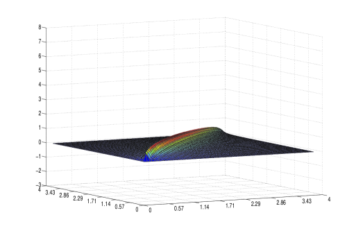
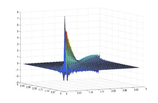
Figure 1: Operator $\psi\left(\cdot,\cdot\right)$ associated with the autocorrelation operator $\rho$, valued at the grid $\left[a,b\right]\times\left[a,b\right]$, for pseudo-diagonal (on left) and non-diagonal (on right) scenarios (see Table 1). Discretization step $\Delta t=0.06$ and shape parameter $\delta_{1}=3/2$ are adopted.

Large-sample behaviour of the ARH(1) plug-in predictors

Large-sample behaviour of the ARH(1) plug-in predictor formulated in Section 8.3, as well as those ones in Bosq (2000) and Guillas (2001) (see equations (3) and (7) above, respectively), will be illustrated. Remark that the ARH(1) plug-in predictor established in Section 8.3 will be only considered under diagonal scenarios. Strong-consistency results for the estimator $\widetilde{\rho}_{k_{n}}$, in the trace norm, when $\rho$ is a positive and trace operator, which does not admit a diagonalization in terms of the eigenvectors of $C$, have been recently provided in Ruiz-Medina & Álvarez-Liébana (2017b). See also Section S.3 of the Supplementary Material, where an almost sure upper bound for $\left\|\widetilde{\rho}_{k_{n}}-\rho\right\|_{\mathcal{S}(H)}^{2}$ is theoretically derived, when $\rho$ is not assumed to admit a diagonal spectral representation, nor to be a trace operator, but it is assumed to be a Hilbert-Schmidt operator.

As commented earlier (see equation (3) above), Assumptions A1, A3 and A5, jointly with the boundedness of $X_{0}$ and the Hilbert-Schmidt assumption of $\rho$, are required in the strong-consistency results by Bosq (2000). Condition (49) was also imposed in that work. From Bosq (2000, Example 8.6), conditions therein considered are held under any scenario in which the truncation parameter $k_{n}=\lceil\log(n)\rceil$ is adopted, under Assumptions A1-A3 and A5 (it can be proved as condition (48) is also verified when $k_{n}=\lceil\log(n)\rceil$). In the formulation of mean-square convergence, Guillas also considered Assumptions A1, A3 and A5. From Guillas (2001, Theorem 2, Example 4), if the regularization sequence above-referred (see equation (7)) verifies $\alpha\frac{C_{k_{n}}^{\gamma}}{n^{\epsilon}}\leq u_{n}\leq\beta C_{k_{n}}$, for $0<\beta<1$ and $\alpha>0$, with $\gamma=1$ and $\epsilon=0$, then the mean-square consistency is achieved under a suitable truncation parameter. In particular, if $k_{n}=\lceil e^{\prime}n^{1/\left(8\delta_{1}+2\right)}\rceil$, with $e^{\prime}=17/10$, the rate of convergence in quadratic mean is of order of $n^{-\delta_{1}/\left(4\delta_{1}+1\right)}$. Remark that, since $\lceil\left(17/10\right)n^{1/\left(8\delta_{1}+2\right)}\rceil<\lceil\ln(n)\rceil$ for $n$ large enough, conditions (48)-(49) are also verified when $k_{n}=\lceil e^{\prime}n^{1/\left(8\delta_{1}+2\right)}\rceil$, with $e^{\prime}=17/10$, is fixed.

For sample sizes $n_{t}=35000+40000\left(t-1\right),\leavevmode\nobreak\ t=1,\ldots,10$, and a suitable truncation parameter $k_{n}$,

$$F\left(k_{n},n_{t},\beta\right)=\left(\displaystyle\sum_{l=1}^{N}\mathbf{1}_{\left(\xi_{n_{t},\beta},\infty\right)}\left(\left\|\left(\rho-\overline{\rho}_{k_{n}}^{l}\right)\left(X_{n-1}^{l}\right)\right\|_{H}^{k_{n}}\right)\right)/N,$$ (52)

will be displayed (see Figures 2-4 below), being $\mathbf{1}_{\left(\xi_{n_{t},\beta},\infty\right)}$ the indicator function over the interval $\left(\xi_{n_{t},\beta},\infty\right)$, where $\xi_{n_{t},\beta}$ numerically fits the almost sure rate of convergence of $\left\|\left(\rho-\overline{\rho}_{k_{n}}^{l}\right)\left(X_{n-1}^{l}\right)\right\|_{H}^{k_{n}}$ (see Tables 2-3 below). When the data is generated in the diagonal framework,

$$\left\|\left(\rho-\overline{\rho}_{k_{n}}^{l}\right)\left(X_{n-1}^{l}\right)\right\|_{H}^{k_{n}}=\sqrt{\displaystyle\int_{a}^{b}\left(\displaystyle\sum_{j=1}^{k_{n}}\rho_{j}X_{n-1,j}^{l}\phi_{j}(t)-\displaystyle\sum_{j=1}^{k_{n}}\overline{\rho}_{n,j}^{l}\left(X_{n-1}^{l}\right)\phi_{n,j}^{l}(t)\right)^{2}dt},$$ (53)

is computed, being $\overline{\rho}_{k_{n}}^{l}\left(X_{n-1}^{l}\right)$ the predictors defined in (44)-(47), (3) and (7), respectively, for any $j=1,\ldots,k_{n}$, and based on the $l$th generation of the values $\widetilde{X}_{i,j}^{l}=\langle X_{i}^{l},\phi_{n,j}^{l}\rangle_{H}$, for $l=1,\ldots,N$, with $N=500$ simulations. The following parameter values will be considered, when the diagonal data generation is assumed:

Table 2: Diagonal scenarios considered (see Figure 2 below, and Table 4 in the Supplementary Material), with $\delta_{2}=11/10$, $n_{t}=35000+40000(t-1),\leavevmode\nobreak\ t=1,\ldots,10$, and $\xi_{n_{t},\beta}=\frac{\left(\ln(n_{t})\right)^{\beta}}{n_{t}^{1/2}}$, for $\beta=65/100$.

Scenario	$\delta_{1}$	$k_{n}$
1	$3/2$	$\lceil\ln(n)\rceil$
2	$24/10$	$\lceil\ln(n)\rceil$
3	$3/2$	$\lceil e^{\prime}n^{1/\left(8\delta_{1}+2\right)}\rceil,\leavevmode\nobreak\ e^{\prime}=17/10$
4	$24/10$	$\lceil e^{\prime}n^{1/\left(8\delta_{1}+2\right)}\rceil,\leavevmode\nobreak\ e^{\prime}=17/10$

As discussed, conditions formulated in Bosq (2000) and Proposition 2 of the current paper are held for scenarios 1-2 in Table 2, while in scenarios 3-4, the conditions assumed in Proposition 2 and the approaches by Bosq (2000) and Guillas (2001), are verified (but not in an optimal sense).

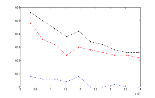
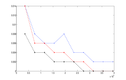
Figure 2: $F\left(k_{n},n_{t},\beta\right)$ values, for scenario 2 (on left) and scenario 4 (on right), for our approach (blue star dotted line) and those one presented in Bosq (2000) (red circle dotted line) and Guillas (2001) (black diamond dotted line). The curve $\xi_{n_{t},\beta}=\frac{\left(\ln(n_{t})\right)^{\beta}}{n_{t}^{1/2}}$, with $\beta=65/100$, is adopted.

Under pseudo-diagonal and non-diagonal frameworks, the following truncated norm is then computed, instead of (53):

$$\left\|\left(\rho-\overline{\rho}_{k_{n}}^{l}\right)\left(X_{n-1}^{l}\right)\right\|_{H}^{k_{n}}=\sqrt{\displaystyle\int_{a}^{b}\left(\displaystyle\int_{a}^{b}\left(\displaystyle\sum_{j,k=1}^{k_{n}}\rho_{j,k}\phi_{j}(t)\phi_{k}(s)\right)ds-\displaystyle\sum_{j=1}^{k_{n}}\overline{\rho}_{n,j}^{l}\left(X_{n-1}^{l}\right)\phi_{n,j}^{l}(t)\right)^{2}dt}.$$ (54)

Pseudo-diagonal and non-diagonal scenarios, for approaches formulated in Bosq (2000) and Guillas (2001), are outlined in Table 3.

Table 3: Pseudo-diagonal and non-diagonal scenarios considered (see Figures 3-4 below, and Tables 5-6 in the Supplementary Material), with $\delta_{2}=11/10$, $n_{t}=35000+40000(t-1),\leavevmode\nobreak\ t=1,\ldots,10$, and $\xi_{n_{t},\beta}=\frac{\left(\ln(n_{t})\right)^{\beta}}{n_{t}^{1/3}}$.

Pseudo-diagonal scenarios				Non-diagonal scenarios
Scenario	$\delta_{1}$	$k_{n}$	$\beta$	Scenario	$\delta_{1}$	$k_{n}$	$\beta$
5	$3/2$	$\lceil\ln(n)\rceil$	$3/10$	9	$3/2$	$\lceil\ln(n)\rceil$	$125/100$
6	$24/10$	$\lceil\ln(n)\rceil$	$3/10$	10	$24/10$	$\lceil\ln(n)\rceil$	$125/100$
7	$3/2$	$\lceil(17/10)n^{1/\left(8\delta_{1}+2\right)}\rceil$	$3/10$	11	$3/2$	$\lceil(17/10)n^{1/\left(8\delta_{1}+2\right)}\rceil$	$125/100$
8	$24/10$	$\lceil(17/10)n^{1/\left(8\delta_{1}+2\right)}\rceil$	$3/10$	12	$24/10$	$\lceil(17/10)n^{1/\left(8\delta_{1}+2\right)}\rceil$	$125/100$

Scenarios 5-6 and 9-10 verify conditions required in Bosq (2000), while scenarios 7-8 and 11-12 are included in both setting of conditions, proposed in Bosq (2000) and Guillas (2001).

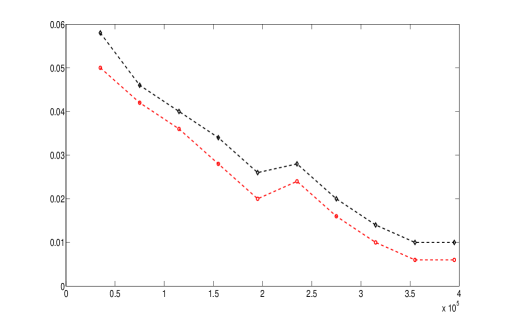
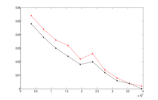
Figure 3: $F\left(k_{n},n_{t},\beta\right)$ values, for scenario 6 (on left) and scenario 8 (on right), for approaches presented in Bosq (2000) (red circle dotted line) and Guillas (2001) (black diamond dotted line). The curve $\xi_{n_{t},\beta}=\frac{\left(\ln(n_{t})\right)^{\beta}}{n_{t}^{1/3}}$, with $\beta=3/10$, is adopted.

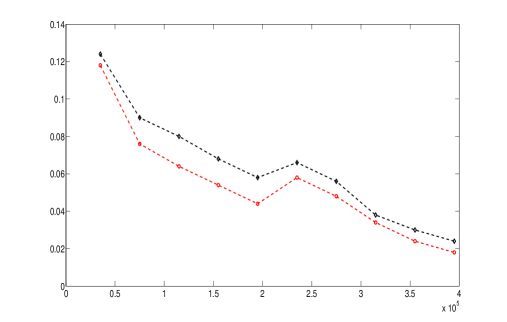
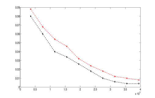
Figure 4: $F\left(k_{n},n_{t},\beta\right)$ values, for scenario 10 (on left) and scenario 12 (on right), for approaches presented in Bosq (2000) (red circle dotted line) and Guillas (2001) (black diamond dotted line). The curve $\xi_{n_{t},\beta}=\frac{\left(\ln(n_{t})\right)^{\beta}}{n_{t}^{1/3}}$, with $\beta=125/100$, is adopted.

Results obtained in the diagonal scenarios 1-4, which are reflected in Table 2, have been applied to the three componentwise ARH(1) plug-in predictor approaches. As expected, the amount of values $\left\|\left(\rho-\overline{\rho}_{k_{n}}^{l}\right)\left(X_{n-1}^{l}\right)\right\|_{H}^{k_{n}}$, which lie within the band $\left[0,\xi_{n_{t},\beta}\right)$, is greater as long as the decay rate of the eigenvalues of $C$ is faster. Since a diagonal framework is considered in scenarios 1-2, a better performance of the approach formulated in Section 8.3 can be noticed in comparison with those ones by Bosq (2000) and Guillas (2001), where errors appear, when sample sizes are not sufficiently large, in the estimation of the non-diagonal componentwise coefficients of $\rho$, which must be zero. This possible effect of the non-diagonal design, under a diagonal scenario, is not observed, for truncation rules selecting a very small number of terms, in relation to the sample size. This fact occurs in the truncation rule adopted in Guillas (2001).

In the pseudo-diagonal and non-diagonal scenarios outlined in Table 3, methodologies in Bosq (2000) and Guillas (2001) are compared, such that the curve $\xi_{n_{t},\beta}=\frac{\left(\ln(n_{t})\right)^{\beta}}{n_{t}^{1/3}}$, for $\beta=3/10$ and $\beta=125/100$, numerically fits their almost sure rate of convergence. As observed (see also Tables 4-6 in Section S.5 of the Supplementary material), the sample-size dependent truncation rule, according to the rate of convergence to zero of the eigenvalues of $C$, plays a crucial role in the observed performance of both approaches.

Small-sample behaviour of the ARH(1) plug-in and non-plug-in predictors

Smaller sample sizes must be adopted in this subsection, since computational limitations arise when regularized wavelet plug-in predictor formulated in Antoniadis & Sapatinas (2003) (see equations (19)-(21) above), as well as penalized predictor and non-parametric kernel-based predictor applied in Besse et al. (2000) (see equations (9) and (33), respectively), are included in the comparative study. See also Section S.5 of the Supplementary Material, where extra numerical results are provided. As above, the diagonal componentwise estimator here formulated will be only considered under diagonal scenarios.

On the one hand, Assumptions A1 and A3, and conditions in (21), are required when regularized-wavelet-based prediction approach is applied. In particular, since $C_{j}=c_{1}j^{-\delta_{1}}$, for any $j\geq 1$, if $k_{n}=\lceil n^{1/\alpha}\rceil$ is adopted, then $1-\frac{4\delta_{1}}{\alpha}>0$, leading to $\alpha>4\delta_{1}$. Additionally to $k_{n}=\lceil\ln(n)\rceil$, the truncation parameter $k_{n}=\lceil n^{1/\alpha}\rceil$ will be adopted (see Table 4-5), with $\alpha=6.5$ and $\alpha=10$, for $\delta_{1}=3/2$ and $\delta_{1}=24/10$, respectively. Furthermore, $F\left(k_{n},n_{t},\beta\right)$ values defined in (52)-(54) are computed for the wavelet-based approach just replacing $\left\{\phi_{n,j},\ j\geq 1\right\}$ by $\left\{\widetilde{\phi}_{j}^{M},\ j\geq 1\right\}$ (see equations (19)-(21)). As before, since $\lceil n^{1/\alpha}\rceil<\lceil\ln(n)\rceil$ and $\lceil n^{1/\alpha}\rceil<\lceil(17/10)n^{1/\left(8\delta_{1}+2\right)}\rceil$, for $\alpha=6.5$ and $\alpha=10$, conditions imposed for the estimator formulated in Section 8, as well as in Bosq (2000) and Guillas (2001), are verified when the truncation parameter $k_{n}=\lceil n^{1/\alpha}\rceil$, with $\alpha=6.5$ and $\alpha=10$, is studied.

On the other hand, let us also compare with the techniques presented in Besse et al. (2000), and detailed in equations (9) and (33), based on penalized prediction and non-parametric kernel-based prediction, respectively. In those techniques, they assume that the functional values of the stationary process are in the Sobolev space $W^{2,2}\left(\left[0,1\right]\right)$. When the referred methodologies in Besse et al. (2000) are implemented, the following alternative norm replaces the norm reflected in (53)-(54), for values $F\left(k_{n},n_{t},\beta\right)$:

$$\left\|\left(\rho-\overline{\rho}_{k_{n}}^{l}\right)\left(X_{n-1}^{l}\right)\right\|_{H} = \sqrt{\displaystyle\int_{a}^{b}\left(\rho\left(X_{n-1}^{l}\right)(t)-\overline{\rho}_{k_{n}}^{l}\left(X_{n-1}^{l}\right)(t)\right)^{2}dt},\quad l=1,\ldots,N.$$ (55)

Hence, the following diagonal scenarios are regarded:

Table 4: Diagonal scenarios considered (see Figure 5 below, and Tables 9-10 in the Supplementary Material), with $M=50$, $q=10$, $\delta_{2}=11/10$, $n_{t}=750+500(t-1),\leavevmode\nobreak\ t=1,\ldots,13$, and $\xi_{n_{t},\beta}=\frac{\left(\ln(n_{t})\right)^{\beta}}{n_{t}^{1/2}},\leavevmode\nobreak\ \beta=65/100$.

Scenario	$\delta_{1}$	$k_{n}$	$h_{n}$
13	$3/2$	$\lceil\ln(n)\rceil$	$0.15,\leavevmode\nobreak\ 0.25$
14	$24/10$	$\lceil\ln(n)\rceil$	$0.15,\leavevmode\nobreak\ 0.25$
15	$3/2$	$\lceil n^{1/\alpha}\rceil,\leavevmode\nobreak\ \alpha=6.5$
16	$24/10$	$\lceil n^{1/\alpha}\rceil,\leavevmode\nobreak\ \alpha=10$

Remark that, since both approaches formulated in Besse et al. (2000) not depend on the truncation parameter $k_{n}$ adopted, we only perform them for scenarios 13-14, where different rates of convergence to zero of the eigenvalues of $C$ are considered, and conditions imposed in that paper are verified. Conditions formulated in Bosq (2000) and Proposition 2 of the current paper are held for all scenarios, while the conditions assumed in Antoniadis & Sapatinas (2003) and Guillas (2001) are only verified under scenarios 15-16.

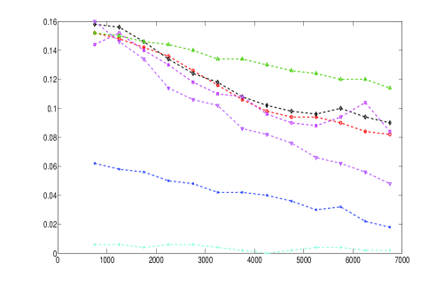
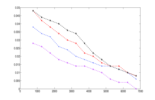
Figure 5: $F\left(k_{n},n_{t},\beta\right)$ values, for scenario 14 (on left) and scenario 16 (on right), for our approach (blue star dotted line) and those one presented in Antoniadis and Sapatinas (2001) (pink square dotted line), Besse et al. (2000) (cyan blue plus dotted line for penalized prediction; dark green upward-pointing triangle and purple downward-pointing triangle dotted lines, for kernel-based prediction, for $h_{n}=0.15$ and $h_{n}=0.25$, respectively), Bosq (2000) (red circle dotted line) and Guillas (2001) (black diamond dotted line). The curve $\xi_{n_{t},\beta}=\frac{\left(\ln(n_{t})\right)^{\beta}}{n_{t}^{1/2}}$, with $\beta=65/100$, is drawn (light green dotted line).

Pseudo-diagonal and non-diagonal scenarios are detailed in Table 5.

Table 5: Pseudo-diagonal and non-diagonal scenarios considered (see Figures 6-7 below, and Tables 11-14 in the Supplementary Material), with $\delta_{2}=11/10$, $n_{t}=750+500(t-1),\leavevmode\nobreak\ t=1,\ldots,13$, and $\xi_{n_{t},\beta}=\frac{\left(\ln(n_{t})\right)^{\beta}}{n_{t}^{1/3}}$.

Pseudo-diagonal scenarios					Non-diagonal scenarios
Scenario	$\delta_{1}$	$k_{n}$	$\beta$	$h_{n}$	Scenario	$\delta_{1}$	$k_{n}$	$\beta$	$h_{n}$
17	$3/2$	$\lceil\ln(n)\rceil$	$3/10$	$1.2,\leavevmode\nobreak\ 1.7$	21	$3/2$	$\lceil\ln(n)\rceil$	$125/100$	$1.2,\leavevmode\nobreak\ 1.7$
18	$24/10$	$\lceil\ln(n)\rceil$	$3/10$	$1.2,\leavevmode\nobreak\ 1.7$	22	$24/10$	$\lceil\ln(n)\rceil$	$125/100$	$1.2,\leavevmode\nobreak\ 1.7$
19	$3/2$	$\lceil n^{1/\alpha}\rceil,\leavevmode\nobreak\ \alpha=6.5$	$3/10$		23	$3/2$	$\lceil n^{1/\alpha}\rceil$	$125/100$
20	$24/10$	$\lceil n^{1/\alpha}\rceil,\leavevmode\nobreak\ \alpha=10$	$3/10$		24	$24/10$	$\lceil n^{1/\alpha}\rceil$	$125/100$

As noted before, approaches formulated in Besse et al. (2000) are only tested for scenarios 17-18 and 21-22, and conditions in Bosq (2000) are verified for all scenarios. Scenarios developed by Antoniadis & Sapatinas (2003) and Guillas (2001) are only held when the truncation parameter proposed in Antoniadis & Sapatinas (2003) is adopted.

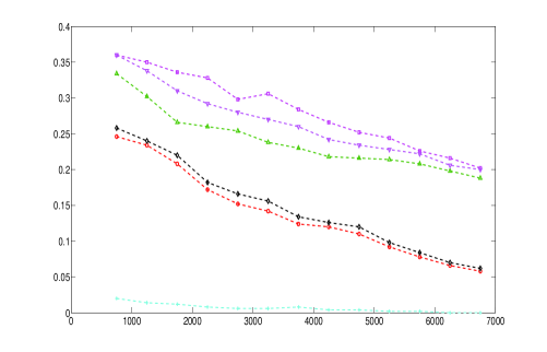
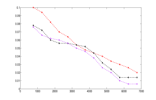
Figure 6: $F\left(k_{n},n_{t},\beta\right)$ values, for scenario 18 (on left) and scenario 20 (on right), for approaches presented in Antoniadis & Sapatinas (2003) (pink square dotted line), Besse et al. (2000) (cyan blue plus dotted line for penalized prediction; dark green upward-pointing triangle and purple downward-pointing triangle dotted lines, for kernel-based prediction, for $h_{n}=1.2$ and $h_{n}=1.7$, respectively), Bosq (2000) (red circle dotted line) and Guillas (2001) (black diamond dotted line). The curve $\xi_{n_{t},\beta}=\frac{\left(\ln(n_{t})\right)^{\beta}}{n_{t}^{1/3}}$, with $\beta=3/10$, is drawn (light green dotted line).

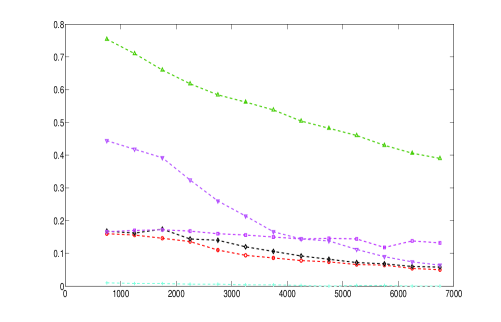
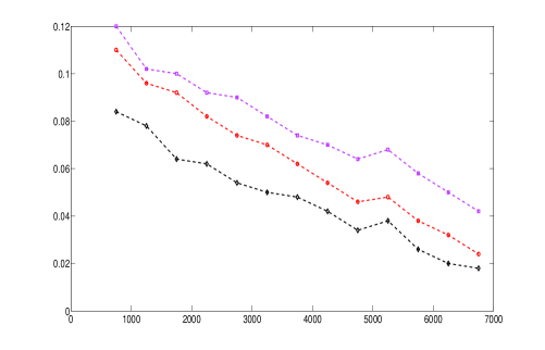
Figure 7: $F\left(k_{n},n_{t},\beta\right)$ values, for scenario 22 (on left) and scenario 24 (on right), for approaches presented in Antoniadis & Sapatinas (2003) (pink square dotted line), Besse et al. (2000) (cyan blue plus dotted line for penalized prediction; dark green upward-pointing triangle and purple downward-pointing triangle dotted lines, for kernel-based prediction, for $h_{n}=1.2$ and $h_{n}=1.7$, respectively), Bosq (2000) (red circle dotted line) and Guillas (2001) (black diamond dotted line). The curve $\xi_{n_{t},\beta}=\frac{\left(\ln(n_{t})\right)^{\beta}}{n_{t}^{1/3}}$, with $\beta=125/100$, is drawn (light green dotted line).

When smaller sample sizes are adopted, and approaches formulated in Antoniadis & Sapatinas (2003) and Besse et al. (2000) are included in the comparative study, scenarios 13-24 have been considered and reflected in Tables 4-5. As expected, the larger sample are used, the better performance is obtained for the empirical-eigenvector-based componentwise approaches tested in the previous subsection. Note that even when small sample sizes are studied, a good performance of the ARH(1) plug-in predictor given in equations (44)-(47) is observed. As well as the regularized wavelet-based approach detailed in Antoniadis & Sapatinas (2003) becomes the best methodology for small sample sizes, in comparision with the componentwise techniques above mentioned.

Note that the good performance observed corresponds to the truncation rule proposed by these authors, with a small number of terms. While, when a larger number of terms is considered, according to the alternative truncation rules tested, the observed outperformance does not hold. While the penalized prediction approach proposed in Besse et al. (2000) has been shown as the more accurate, is, however, less affected by the regularity conditions imposed on the autocovariance kernel (see Tables 9-14 in Section S.5 of the supplementary material). The non-parametric kernel-based purpose by Besse et al. (2000) requires to solve the selection problem associated with the bandwidth parameter. Furthermore, a drawback of both approaches in Antoniadis & Sapatinas (2003) and Besse et al. (2000) is that they require large computational times in their implementations. The underlying dependence structure, given by the covariance operators and their spectral decompositions, cannot be provided in those approaches.

Acknowledgments

This work has been supported in part by project MTM2015–71839–P (co-funded by Feder funds), of the DGI, MINECO, Spain.

References

- [1]
- [2] Allan, A. & Mourid, T. (2014). Covariance operator estimation of a functional autoregressive process with random coefficients. Statist. Probab. Lett., 84, 1–8.
- [3] Álvarez-Liébana, J., Bosq, D. & Ruiz-Medina, M. D. (2016). Consistency of the plug-in functional predictor of the Ornstein-Uhlenbeck process in Hilbert and Banach spaces. Statist. Probab. Lett., 117, 12–22.
- [4] Álvarez-Liébana, J., Bosq, D. & Ruiz-Medina, M. D. (2017). Asymptotic properties of a componentwise ARH(1) plug-in predictor. J. Multivariate Anal., 155, 12–34.
- [5] Andersson, J. & Lillestøl, J. (2010). Modeling and forecasting electricity consumption by functional data analysis. The Journal of Energy Markets, 3, 3–15.
- [6] Antoniadis, A., Brosat, X., Cugliari, J. & Poggi, J. M. (2012). Prévision d’un processus à valeurs fonctionnelles en présence de non stationnarités. Application à la consommation d’électricité. J. SFdS, 153, 52–78.
- [7] Antoniadis, A., Paparoditis, E. & Sapatinas, T. (2006). A functional wavelet-kernel approach for time series prediction. J. R. Stat. Soc. Ser. B. Stat. Methodol., 68, 837–857.
- [8] Antoniadis, A., Paparoditis, E. & Sapatinas, T. (2009). Bandwidth selection for functional time series prediction. Statist. Probab. Lett., 79, 733–740.
- [9] Antoniadis, A. & Sapatinas, T. (2003). Wavelet methods for continuous-time prediction using Hilbert-valued autoregressive processes. J. Multivariate Anal., 87, 133–158.
- [10] Aue, A., Norinho, D. & Hörmann, S. (2015). On the prediction of stationary functional time series. J. Amer. Statist. Assoc., 110, 378–392 .
- [11] Bensmain, N. & Mourid, T. (2001). Estimateur “sieve” de l’opérateur d’un processus ARH. C. R. Acad. Sci. Paris Sér. I Math., 332, 1015–1018.
- [12] Benyelles, W. & Mourid, T. (2001). Estimation de la période d’un processus à temps continu à représentation autorégressive. C. R. Acad. Sci. Paris Sér. I Math., 333, 245–248.
- [13] Besse, P.C. & Cardot, H. (1996). Approximation spline de la prévision d’un processu fonctionnel autoregréssif d’ordre 1. Canad. J. Statist., 24, 467–487.
- [14] Besse, P. C., Cardot, H. & Stephenson, D. B. (2000). Autoregressive forecasting of some functional climatic variations. Scand. J. Stat., 27, 673–687.
- [15] Blanke, D. & Bosq, D. (2014). Exponential bounds for intensity of jumps. Math. Methods Statist., 23, 239–255.
- [16] Bosq, D. (1991). Modelization, non-parametric estimation and prediction for continuous time processes. Nonparametric functional estimation and related topics, NATO, ASI Series, 335, 509–529.
- [17] Bosq, D. (1999a). Autoregressive representation for the empirical covariance operator of an ARH. C. R. Acad. Sci. Paris Sér. I Math., 329, 531–534.
- [18] Bosq, D. (1999b). Autoregressive Hilbertian Processes. Annales de l’ISUP, 43, 25–55.
- [19] Bosq, D. (2000). Linear Processes in Function Spaces. Springer, New York.
- [20] Bosq, D. (2007). General linear processes in Hilbert spaces and prediction. J. Stat. Planning and Inference, 137, 879–894.
- [21] Bosq, D. (2010). Tensorial products of functional ARMA processes. J. Multivariate Anal., 101, 1352–1363.
- [22] Bosq, D. & Blanke, D. (2007). Inference and Predictions in Large Dimensions. Wiley, Chichester.
- [23] Cardot, H. (1998). Convergence du lissage spline de la prévision des processus autorégressifs fonctionnels. C. R. Acad. Sci. Paris Sér. I Math., 326, 755–758.
- [24] Cavallini, A., Montanari, G. C., Loggini, M., Lessi, M. & Cacciari, M. (1994). Nonparametric prediction of harmonic levels in electrical networks. Proceed. IEEE ICHPS VI Bologna, 165–171.
- [25] Chen, S. X., Lei, L. & Tu, Y. (2016). Functional coefficient moving average model with applications to forecasting chinese CPI. Statist. Sinica, 26, 1649–1672.
- [26] Cuevas, A., Febrero, M. & Fraiman, R. (2002). Linear functional regression: the case of fixed design and functional response. Canad. J. Statist., 30, 285–300.
- [27] Cugliari, J. (2011). Prévision non paramétrique de processus à valeurs fonctionnelles. Application à la consommation d’électricité. PhD thesis, University of Paris-Sud 11, Paris.
- [28] Cugliari, J. (2013). Conditional Autoregressive Hilbertian processes. arXiv:1302.3488.
- [29] Damon, J. & Guillas, S. (2002). The inclusion of exogenous variables in functional autoregressive ozone forecasting. Environmetrics, 13, 759–774.
- [30] Damon, J. & Guillas, S. (2005). Estimation and simulation of autoregressive processes with exogenous variables. Stat. Inference Stoch. Process., 8, 185–204.
- [31] Dedecker, J. & Merlevède, F. (2002). Necessary and sufficient conditions for the conditional central limit theorem. Ann. Probab., 30, 1044–1081.
- [32] Dedecker, J. & Merlevède, F. (2003). The conditional central limit theorem in Hilbert spaces. Stochastic Process. Appl., 108, 229–262.
- [33] Dehling, H. & Sharipov, O. S. (2005). Estimation of mean and covariance operator for Banach space valued autoregressive processes with dependent innovations. Stat. Inference Stoch. Process., 8, 137–149.
- [34] Didericksen, D., Kokoszka, P. & Zhang, X. (2012). Empirical properties of forecast with the functional autoregressive model. Comput. Stat., 27, 285–298.
- [35] Ferraty, F., Van Keilegom, I. & Vieu, P. (2012). Regression when both response and predictor are functions. J. Multivariate Anal., 109, 10–28.
- [36] Ferraty, F. & Vieu, P. (2006). Nonparametric functional data analysis: Theory and practice. Springer, Berlin.
- [37] Fortet, R. (1995). Vecteurs, fonctions et distributions aleatoires dans les espaces de Hilbert. Hermes, Paris.
- [38] Grenander, U. (1981). Abstract Inference. Wiley, New York.
- [39] Guillas, S. (2000). Noncausality and functional discretization, limit theorems for an ARHX process. C. R. Acad. Sci. Paris Sér. I Math., 331, 91–94.
- [40] Guillas, S. (2001). Rates of convergence of autocorrelation estimates for autoregressive Hilbertian processes. Statist. Probab. Lett., 55, 281–291.
- [41] Guillas, S. (2002). Doubly stochastic Hilbertian processes. J. Appl. Probab., 39, 566–580.
- [42] El Hajj, L. (2011). Limit theorems for -valued autoregressive processes. C. R. Acad. Sci. Paris Sér. I Math., 349, 821–825.
- [43] El Hajj, L. (2013). Inférence statistique pour des variables fonctionnelles à Sauts. PhD thesis, University Paris VI, Paris.
- [44] Hörmann, S., Horváth, L. & Reeder, R. (2013). A functional version of the ARCH model. Econometric Theory, 29, 267–288.
- [45] Hörmann, S., Kidziński, L. & Hallin, M. (2015). Dynamic functional principal components. J. R. Stat. Soc. Ser. B. Stat. Methodol., 77, 319–348.
- [46] Hörmann, S. & Kidziński, L. (2015). A Note on Estimation in Hilbertian Linear Models. Scand. J. Stat., 42, 43–62.
- [47] Hörmann, S. & Kokoszka, P. (2010). Weakly dependent functional data. Ann. Statist., 38, 1845–1884.
- [48] Horváth, L., Husková, M. & Kokoszka, P. (2010). Testing the stability of the functional autoregressive process. J. Multivariate Anal., 101, 352–367.
- [49] Horváth, L., Kokoszka, P. & Rice, G. (2014). Testing stationarity of functional time series. J. Econometrics, 179, 66–82.
- [50] Hyndman, R. J. & Shang, H. L. (2008). Bagplots, Boxplots and Outlier Detection for Functional Data. In: Functional and Operatorial Statistics. Contributions to Statistics. Physica-Verlag HD.
- [51] Hyndman, R. J. & Shang, H. L. (2009). Forecasting functional time series. J. Korean Statist. Soc., 38, 199–211.
- [52] Hyndman, R. J. & Ullah, Md. S (2007). Robust forecasting of mortality and fertility rates: A functional data approach. Comput. Statist. Data Anal., 51, 4942–4956.
- [53] Kara-Terki, N. & Mourid, T. (2016). Local asymptotic normality of Hilbertian autoregressive processes. C. R. Acad. Sci. Paris Sér. I, 354, 634–638.
- [54] Kargin, V. & Onatski, A. (2008). Curve forecasting by functional autoregression. J. Multivariate Anal., 99, 2508–2526.
- [55] Kokoszka, P., Maslova, I., Sojka, J. & Zhu, L. (2008). Testing for lack of dependence in the functional linear model. Canad. J. Statist., 36, 207–222.
- [56] Kokoszka, P. & Reimherr, M. (2013a). Asymptotic normality of the principal components of functional time series. Stochastic Process. Appl., 123, 1546–1562.
- [57] Kokoszka, P. & Riemherr, M. (2013b). Determining the order of the functional autoregressive model. J. Time Series Anal., 34, 116–129.
- [58] Kowal, D. R., Matteson, D. S. & Ruppert, D. (2017). Functional autoregression for sparsely sample data. J. Bus. Econom. Statist., to appear.
- [59] Kuelbs, J. (1976). A strong convergence theorem for Banach valued random variables. Ann. Prob., 4, 744–771.
- [60] Labbas, A. & Mourid, T. (2002). Estimation et prévision d’un processus autorégressif Banach. C. R. Acad. Sci. Paris Sér. I, 335, 767–772.
- [61] Laukaitis, A. & Rac̆kauskas, A. (2002). Functional data analysis of payment systems. Nonlinear Anal. Model. Control, 7, 53–68.
- [62] Mallat, S. G. (1989). A theory of multiresolution signal decomposition: the wavelet representation. IEEE Trans. Pattn. Anal. Mach. Intell., 11, 674–693.
- [63] Marion, J.-M. & Pumo, B. (2004). Comparison of ARH and ARHD models on physiological data. Ann. I.S.U.P., 48, 29–38.
- [64] Martin, D. E. K. (1982). Estimation of the minimal period of periodically correlated sequences. Ph. D. Thesis. University of Maryland, Maryland.
- [65] Mas, A. (1999). Normalité asymptotique de l’estimateur empirique de l’opérateur d’autocorrélation d’un processus ARH. C. R. Acad. Sci. Paris Sér. I Math., 329, 899–902.
- [66] Mas, A. (2000). Estimation d’opérateurs de corrélation de processus fonctionnels: lois limites, tests, déviations modérées. Ph. D. Thesis. University of Paris VI, France.
- [67] Mas, A. (2002). Weak convergence for the covariance operators of a Hilbertian linear process. Stochastic Process. Appl., 99, 117–135.
- [68] Mas, A. (2004). Consistance du prédicteur dans le modèle ARH: le cas compact. Ann. I.S.U.P., 48, 39–48.
- [69] Mas, A. (2007). Weak-convergence in the functional autoregressive model. J. Multivariate Anal., 98, 1231–1261.
- [70] Mas, A. & Menneteau, L. (2003a). Large and moderate deviations for infinite dimensional autoregressive processes. J. Multivariate Anal., 87, 241–260.
- [71] Mas, A. & Menneteau, L. (2003b). Perturbation approach applied to the asymptotic study of random operators. Progress in Probability, 55, 127–134.
- [72] Mas, A. & Pumo, B. (2007). The ARHD model. J. Statist. Plann. Inference, 137, 538–553.
- [73] Menneteau, L. (2005). Some laws of the iterated logarithm in Hilbertian autoregressive models. J. Multivariate Anal., 92, 405–425.
- [74] Merlevède, F. (1995). Sur l’inversibilité des processus linéaires à valeurs dans un espace de Hilbert. C. R. Acad. Sci. Paris, Sér. I, 321, 477–480.
- [75] Merlevède, F. (1996). Central limit theorem for linear processes with values in a Hilbert space. Stochastic Process. Appl., 65, 103–114.
- [76] Merlevède, F. (1997). Résultats de convergence presque sûre pour l’estimation et la prévision des processus linéaires hilbertiens. C. R. Acad. Sci. Paris, Sér. I, 324, 573–576.
- [77] Merlevède, F., Peligrad, M. & Utev, S. (1997). Sharp Conditions for the CLT of Linear Processes in a Hilbert Space. J. Theoret. Probab. , 10, 681–693.
- [78] Meyer, Y. & Coifman, R. (1997). Wavelets, Calderón-Zygmund and Multilinear Operators. Cambridge University Press, Cambridge.
- [79] Mokhtari, F. & Mourid, T. (2003). Prediction of continuous time autoregressive processes via the Reproducing Kernel Spaces. Stat. Inference Stoch. Process., 6, 247–266.
- [80] Mourid, T. (1993). Processus autorégressifs banachiques d’ordre supérieur. C. R. Acad. Sci. Paris Sér. I Math., 317, 1167–1172.
- [81] Mourid, T. (1996). Représentation autorégressive dans un espace de Banach de processus réels à temps continu et équivalence des lois. C. R. Acad. Sci. Paris Sér. I Math., 322 , 1219-1224.
- [82] Mourid, T. (2004). Processus autorégressifs hilbertiens à coefficients aléatoires. Ann. I.S.U.P., 48, 79–85.
- [83] Panaretos, V. M. & Tavakoli, S. (2013). Cramér-Karhunen-Loève representation and harmonic principal component analysis of functional time series. Stoch. Processes Appl., 123, 2779–2807.
- [84] Parvardeh, A., Mohammadi, N., Mahmoodi, S. & Soltani, A. R. (2017). First order autoregressive periodically correlated model in Banach spaces: existence and central limit theorem. J. Multivariate Anal., 449, 756–768.
- [85] Parzen, E. (1961). An approach to time series analysis. Ann. Math. Statist., 32, 951–989.
- [86] Poggi, J. M. (1994). Prévision non paramétrique de la consommation électrique. Revue de Statistique Appliquée, 42, 93–98.
- [87] Pumo, B. (1992). Estimation et prévision de processus autorégressifs fonctionnels. PhD thesis, Université de Paris 6, Paris.
- [88] Pumo, B. (1998). Prediction of continuous time processes by -valued autoregressive process. Stat. Inference Stoch. Process. , 1, 297–309.
- [89] Rachedi, F. (2005). Estimateurs cribles des processus autorégressifs Banachiques. PhD Thesis, Université Pierre et Marie Curie - Paris VI, Paris.
- [90] Reiss, P. T. & Ogden, T. (2007). Functional principal component regression and functional partial least-squares. J. Amer. Statist. Assoc., 102, 984–996.
- [91] Ruiz-Medina, M. D. (2011). Spatial autoregressive and moving average Hilbertian processes. J. Multivariate Anal., 102, 292–305.
- [92] Ruiz-Medina, M. D. (2012). Spatial functional prediction from spatial autoregressive Hilbertian processes. Environmetrics 23, 119–128.
- [93] Ruiz-Medina, M. D. & Álvarez-Liébana, J. (2017a). Classical and Bayesian componentwise predictors for non-ergodic ARH(1) processes. REVSTAT, in press.
- [94] Ruiz-Medina, M. D. & Álvarez-Liébana, J. (2017b). Consistent diagonal componentwise ARH(1) prediction. Submitted.
- [95] Soltani, A. R. & Hashemi, M. (2011). Periodically correlated autoregressive Hilbertian processes. Stat. Inference Stoch. Process., 14, 177–188.
- [96] Spangenberg, F. (2013). Strictly stationary solutions of ARMA equations in Banach spaces. J. Multivariate Anal., 121, 127–138.
- [97] Turbillon, C., Bosq, D., Marion, J. M. & Pumo, B. (2008). Estimation du paramètre des moyennes mobiles hilbertiennes. C. R. Acad. Sci. Paris Sér. I Math., 346, 347–350.
- [98] Wang, H.B. (2008). Nonlinear ARMA models with functional MA coefficients. J. Time Series Anal., 29, 1032–1056.