A Bayesian algorithm for detecting identity matches
and fraud in image databases

Abstract

A statistical algorithm for categorizing different types of matches and fraud in image databases is presented. The approach is based on a generative model of a graph representing images and connections between pairs of identities, trained using properties of a matching algorithm between images.

1 Introduction

This report describes a machine learning algorithm for detecting and classifying different types of identity fraud, developed as part of Digital Signal Corporation’s DCAF 2.0 product and service (Database Conversion and the Analysis of Fraud). In this context, detecting identity fraud amounts to finding different types of connections between pairs of identities (IDs) across databases of IDs, each containing various types of images of faces. The algorithm is based on a probabilistic, generative model of a graph representing all images in a pair of IDs, coupled with an image matcher, or a program that produces a similarity score between $0$ and $1$ for any pair of images. The fraud detection algorithm takes advantage of known statistics of the matcher on a training dataset and directly computes likelihoods of several types of fraud that a system operator would be interested in, without producing or relying on any intermediate feature, which results in a highly accurate and nearly optimal classifier.

The scenario addressed by the algorithm can be described as follows. We have a collection of $P$ IDs, the probe, to be tested against a (typically much larger) database of $G$ IDs, the gallery. Each ID consists of a collection of 2D images and/or 3D meshes taken from DSC’s laser imaging system, although for clarity, the results in this report discuss 2D images only. A person approaches a checkpoint with an ID card containing several existing images of his or her face, and the system collects one or more additional images of the face to add to the ID, forming the probe. This may also be repeated for a sequence of individuals, each having their own ID, to form a larger probe with $P>1$. The gallery is an existing database of IDs previously collected by the system in this manner. For each pair of a probe ID and a gallery ID, the classifier determines if there is a match, and if so, what the nature of the match is. For example, the two IDs might actually be the same individual and all of the images within them would be (approximately) the same, or the person could have possession of someone else’s ID card, so that it does not match their own face but instead matches another ID in the gallery database. This matching process is performed on all $PG$ pairs of IDs, and the outputs are a $P\times G$ matrix of decisions as well as a numerical score for each pair that was identified as fraud, indicating how strong that result was. For each fraud type of interest, a ranked list of probe-gallery ID pairs with the top scores are submitted to an operator for further inspection. The subsequent sections of this report describe the different types of identity fraud the system looks for, the mathematical and statistical framework used to model these classes, and various performance tests and simulations.

2 Types of identity fraud

Let $R$ be the edges of the observed graph, consisting of a probe ID and a gallery ID with vertices $V_{1}$ and $V_{2}$ respectively. Let $E_{1}$ and $E_{2}$ be the edges within the probe and gallery IDs and $E_{1,2}$ be the edges between the two IDs, so that $R=E_{1}\cup E_{2}\cup E_{1,2}$. The vertices represent images and the edges are the matcher scores between pairs of images, which are assumed to be between $0$ and $1$. Note that if $|V_{1}|=N_{P}$ and $|V_{2}|=N_{G}$, where $|\cdot|$ is the size of a set, then we can calculate the total number of edges in $R$ as $\frac{1}{2}N_{P}(N_{P}-1)+\frac{1}{2}N_{G}(N_{G}-1)+N_{P}N_{G}$. Given $R$, the classifier is built to distinguish between seven possible hypotheses $H$, including a baseline “no fraud” case and six different types of fraud.

The “No fraud” case, $H=1$, is the situation where the probe and gallery subgraphs are each complete and also fully disjoint from each other. This is the baseline case that we would expect to see when the two IDs are in fact different people. “Multi-ID,” or $H=2$, is the case where both subgraphs are complete and fully connected to each other, i.e. the two IDs are actually the same person. “Probe mismatch,” $H=3$, is the case when the probe subgraph is incomplete, but the two IDs are fully disjoint from each other. This represents a situation where the probe ID contains fraudulent images, but the gallery ID has no involvement in the fraud, and we must look at other gallery IDs to locate the match. “Probe mixed-ID,” $H=4$, is similar to $H=3$ but where the vertices that are disjoint in the probe subgraph have full connections to every image in the gallery subgraph. This occurs when we have found the gallery ID that the mismatched images in the probe ID belong to. “Gallery mismatch,” $H=5$, and “Gallery mixed-ID,” $H=6$, are the same as $H=3$ and $H=4$ respectively but with the roles of the probe and gallery reversed. Note that the interpretation of $H=5$ can vary in practice. It is not necessarily a situation we want to call fraud (especially if we are only interested in finding fraud within the probe ID) but it has a fairly high probability of occurring in practice, and needs to be accounted for by the classifier to obtain accurate results with the other hypotheses. The final case, “Crossed ID” or $H=7$, occurs when both subgraphs are incomplete, but there are two disjoint linkages between them. It corresponds to a scenario where a group of people (such as a family) is enrolling under multiple IDs. Examples of the seven hypotheses are shown in Figure 1 for an ID pair with two images in each ID.

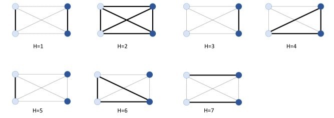
Figure 1: The seven hypotheses that the classifier chooses between, for a (2,2) ID pair. The vertices on the left are in the probe ID and the ones on the right are in the gallery ID.

Note that these hypotheses describe the underlying ground truth on the graph. Due to the slight inaccuracy and randomness of the matcher, it is possible for “nonphysical” data to be actually observed in practice, such as a case with three images, A, B and C, where the edges A-B and B-C have scores of 0.9, but A-C has a score of 0.1. The classifier will still map this observation to the hypothesis $H$ that is the best match to the data. It should also be remarked that the seven hypotheses do not cover every possible ground truth. For example, one can imagine a case similar to $H=7$ where there are three or more disjoint linkages. However, in practice we expect that cases like this have a very low probability of occurring, and even when they do occur, the classifier will still select the “closest” hypothesis, usually $H=7$.

This type of graph is formed for every pair between the $P$ probe IDs and $G$ gallery IDs, and the resulting $PG$ problems are largely treated independently of each other. Note that in many other contexts, similar types of matching problems are typically addressed by using hash tables, reducing the $PG$ ID comparisons to a number on the order of $P+G$. However, in the scenario we address here, the matcher scores and classifier outputs are approximate and real-valued. Conventional hash functions preserve exact matches between data but by design, fail to preserve close distances between data, and thus are not applicable.

3 Theory and statistical model

We assume we are given $p_{M}$ and $p_{N}$, the match and non-match sample densities of the image matcher. These statistics may come from the same probe and/or gallery dataset that we are testing for fraud in, or from a separate, training gallery dataset. The training data only consists of the matcher outputs for pairs of matching and non-matching images, and does not require any information about fraud. The sample statistics are formed using histograms of the data with $CN^{1/3}/\sigma$ bins for $N$ samples, where $C$ is some constant and $\sigma$ is the sample standard deviation; several rules of this type exist in the statistics literature and have various optimality properties. Smoother density estimates such as those based on Gaussian or wavelet kernels were investigated, but turned out to be less well suited than histograms for capturing the sharp spikes that typically appear in these densities (see Figure 2).

We now make the assumption that the scores on every edge are independent, similar to a naive Bayes classifier. This is an approximation and is not the case in practice, but it turns out to affect all the hypotheses roughly equally and does not significantly impact the classifier’s accuracy. The likelihood function of $R$ under each hypothesis is not easy to estimate directly, but this assumption allows us to express it entirely in terms of the densities $p_{M}$ and $p_{N}$. We define $V_{1},V_{2},E_{1},E_{2},E_{1,2}$ as in the previous section, with $R=E_{1}\cup E_{2}\cup E_{1,2}$. For any collection of vertices $V$, we also denote the reduced power set (collection of all subsets, except the empty set and the entire set) of $V$ by $2^{V}-2$, and the set of edges in the complete graph on $V$ by $E(V)$. Note that $|2^{V}-2|=2^{|V|}-2$. Furthermore, for any collection of edges $E\subset R$, define the match likelihood on those edges by

$$L(E)=\left(\prod_{E_{i}\in E}p_{M}(E_{i})\right)\left(\prod_{E_{i}\in R\backslash E}p_{N}(E_{i})\right).$$

The classifier first computes the likelihoods $p(R|H=h)$ for each of the seven hypotheses $h$. The likelihoods are given by the following formulas.

$$p(R|H=1) = L(E_{1}\cup E_{2})$$

$$p(R|H=2) = L(E_{1}\cup E_{2}\cup E_{1,2})$$

$$p(R|H=3) = \frac{1}{|2^{V_{1}}-2|}\sum_{S\in 2^{V_{1}}-2}L(E(S)\cup E_{2})$$

$$p(R|H=4) = \frac{1}{|2^{V_{1}}-2|}\sum_{S\in 2^{V_{1}}-2}L(E(S)\cup E(V_{1}\backslash S\thinspace\cup\thinspace V_{2}))$$

$$p(R|H=5) = \frac{1}{|2^{V_{2}}-2|}\sum_{S\in 2^{V_{2}}-2}L(E(S)\cup E_{1})$$

$$p(R|H=6) = \frac{1}{|2^{V_{2}}-2|}\sum_{S\in 2^{V_{2}}-2}L(E(S)\cup E(V_{2}\backslash S\thinspace\cup\thinspace V_{1}))$$

$$p(R|H=7) = \frac{1}{|2^{V_{1}}-2||2^{V_{2}}-2|}\sum_{S_{1}\in 2^{V_{1}}-2}\sum_{S_{2}\in 2^{V_{2}}-2}L(E(S_{1}\cup V_{2}\backslash S_{2})\cup E(S_{2}\cup V_{1}\backslash S_{1}))$$

Note that these formulas match the structure of the hypotheses in Figure 1. For example, under $H=1$, the likelihood function reflects the fact that we expect $E_{1}$ and $E_{2}$ to all be matches and $E_{1,2}$ to all be non-matches. The sums run over all possible subsets of fraudulent images within each ID, that correspond to valid cases under the given hypothesis. The number of terms grows exponentially large with the number of images, making the likelihoods potentially expensive to compute. One way to simplify this problem is to not consider all elements in $2^{V}-2$, but restrict the sums to subsets containing at most $M$ elements for some fixed $M$, i.e. only considering cases where any given ID has at most $M$ fraudulent images. The effect of this approximation will be investigated in the next section, but it turns out to be a reasonable assumption in practice, where even large IDs typically contain at most only a few mismatched images. In practice, the vertices and indices corresponding to each element of the reduced power set can be stored in a lookup table and reused across different pairs of identities, and ordered by the size of each subset using the “revolving door algorithm” based on Pascal’s triangle.

Once the likelihoods are computed, they can be used to make a decision $D$ about $H$ according to one of several standard optimality criteria: the maximum likelihood (ML), maximum a posteriori (MAP) or minimum mean square (MMS) estimates, which correspond to the following choices for $D$.

$$D_{\mathrm{ML}} = \arg\max_{h}p(R|H=h)$$

$$D_{\mathrm{MAP}} = \arg\max_{h}p(R|H=h)p(H=h)$$

$$D_{\mathrm{MMS}} = \mathrm{round}\bigg{(}\frac{\sum_{h=1}^{7}hp(R|H=h)p(H=h)}{\sum_{h=1}^{7}p(R|H=h)p(H=h)}\bigg{)}$$

Note that $D_{\mathrm{MMS}}$ is effectively an average and depend on what order the 7 classes are in (i.e. which one is $H=1$, $H=2$ and so on). $D_{\mathrm{MAP}}$ corresponds to the so-called naive Bayes classifier, and is the one the DCAF system uses in practice. If the priors $p(H=h)$ were all equal for $1\leq h\leq 7$, then $D_{\mathrm{MAP}}=D_{\mathrm{ML}}$, but the “no fraud” $p(H=1)$ probability is typically much larger than any of the other cases on common training datasets.

Once the algorithm makes a decision $D$, the log-likelihood of the corresponding hypothesis $\log p(G|H=D)$ is used as a numerical score of how strongly fraudulent that pair of IDs is, relative to other pairs of IDs. These scores are then used to produce a list of the most strongly fraudulent pairs of IDs. In practice, this log-likelihood is divided by the total number of edges in the graph to produce a score that is independent of the number of images in the ID.

4 Performance and simulation results

This section summarizes some results on the performance of the classifier under different constraints and datasets. The densities $p_{M}$ and $p_{N}$ are estimated from the outputs of a commercial 2D image matcher (Cognitec FaceVACS; see [1] and [2]) on every pair of faces in the MORPH face dataset (about $80,000$ face images), which produces $136,000$ match and $231$ million non-match points. Note that the number of non-match points is much larger, as is typical, and its histogram has more bins to account for this. The resulting density estimates are shown in Figure 2.

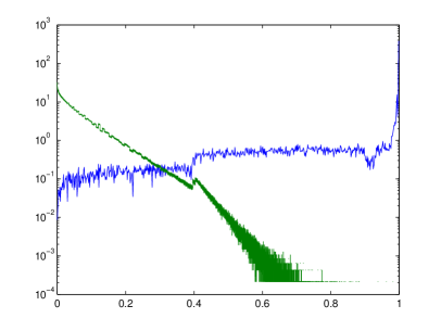
Figure 2: Match (blue) and non-match (green) density estimates from MORPH data under Cognitec.

To test the performance of the classifier, we check the classifier’s decisions on simulated (3,3) ID pairs from several test datasets, i.e. 3 images each in the probe and gallery IDs. The datasets consist of a random subset of MORPH (called MORPH_Rand_10), a dataset of the company employees (DSCEmployee) and an older dataset collected at the University of Notre Dame at 45-degree angle offsets (NDOff45). The MORPH subset contains 900 identities with 10 images each; we treat 100 of these as the probe and the remaining 800 as the gallery. The simulation generates fraudulent ID pairs corresponding to 4 of the 7 hypotheses, $H\in\{1,2,4,6\}$. We restrict our attention to only these fraud cases to allow for a comparison with a legacy algorithm used in DCAF 1.6 to address the same problem, which uses a spectral clustering-based feature and only recognizes these cases [3]. The maximum likelihood decision $D_{\mathrm{ML}}$ is used for the statistical classifier, to account for the fact that the simulation generates an equal number of each of the fraud cases. Note that in a real system where the fraudulent cases are unlikely to begin with, $D_{\mathrm{MAP}}$ with non-uniform priors would be expected to have better performance with lower false positive rates.

The production version of the classifier is implemented in DCAF 2.0 as a C++ module with Python and Matlab APIs. The likelihoods for each probe-gallery ID pair in a database can be computed concurrently and are easily amenable to multithreading or GPU computation. The inputs are matcher scores between the probe and gallery databases and the classifier outputs matcher scores. We set the maximum number of fraudulent images per ID $M=3$, which, as will be seen below, speeds up the calculations by a few orders of magnitude with a minimal effect on the classifier’s accuracy. The 4x4 matrix of classification accuracies between different hypotheses $H$ and decisions $D$ is shown for MORPH_Rand_10 and NDOff45 in Figure 3, for both this technique as well as the clustering method. It can be seen that the statistical algorithm has significantly better accuracy with both datasets, especially in terms of the false positives (the top rows in Figure 3) that are often critical in a real situation. The relative improvement is also greater on NDOff45, a harder dataset to work with due to its greater angle variations, indicating that the classifier performs especially well on borderline cases.

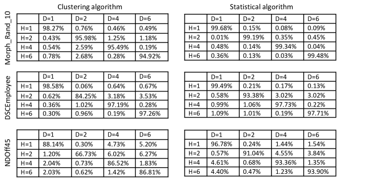
Figure 3: Classification error rates for the spectral clustering method (left) and the statistical method (right) on (3,3) ID pairs from MORPH_Rand_10 (top), DSCEmployee (middle) and NDOff45 (bottom).

For each of these cases, we also examine the distributions of the log-likelihood scores when the classifier reaches the corresponding decision. The plots are shown in Figure 4. The scores generally look like Gaussian variables for most of the hypotheses, typically taking on values between $0$ and $60$ (or $0$ and $4$ after dividing by the number of edges as described earlier), with the exception of cases involving $H=2$ or $D=2$. The exact reasons for this are not well understood, but in the $H=2$, $D=2$ case, this can interpreted to mean that the classifier is always “very sure” of its answer when it correctly detects a multi-ID case.

We finally consider a different type of test in Figure 5, where the classifier is run on MORPH_Rand_10 for different values of $M$, with 80,000 ID pairs to be checked. There is no fraud simulation done here, and the objective is instead to study the false positive rates across all seven hypotheses and to examine the tradeoff with the computation time. An ideal classifier would choose $D=1$ for all 80,000 cases, although in practice, the dataset actually contains a few mislabeled images that would prevent this. It can be seen that the $H=3$ and $H=5$ cases generate a lot of false positives relative to the other cases. There is also zero improvement in going from $M=3$ to $M=4$, despite the large increase in computation time (the time shown is the total for all 80,000 pairs).

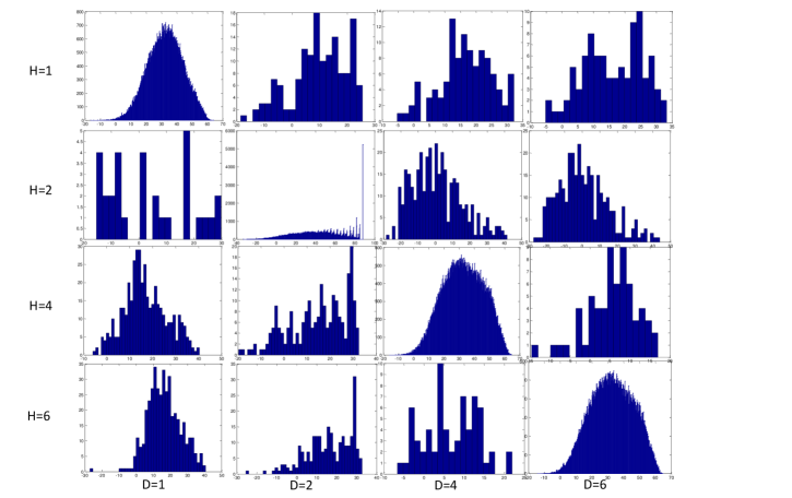
Figure 4: Log-likelihood score densities for different hypotheses and decisions.

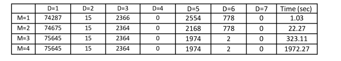
Figure 5: Results of the false positive test on 80,000 (10,10) ID pairs from MORPH_Rand_10 for different values of $M$.

References

- [1] D. Giorgi et al. A Critical Assessment of 2D and 3D Face Recognition Algorithms. Sixth IEEE International Conference on Advanced Video and Signal Based Surveillance, 2009.
- [2] Cognitec Systems GmbH. FaceVACS algorithm performance. http://www.cognitec.com. Accessed in 2014.
- [3] C. Roller. System and method for detecting potential fraud between a probe biometric and a dataset of biometrics, 2015.