Anisotropic Challenges in Pedestrian Flow Modeling

Abstract

Macroscopic models of crowd flow incorporating individual pedestrian choices present many analytic and computational challenges. Anisotropic interactions are particularly subtle, both in terms of describing the correct “optimal” direction field for the pedestrians and ensuring that this field is uniquely defined. We develop sufficient conditions, which establish a range of “safe” densities and parameter values for each model. We illustrate our approach by analyzing several established intra-crowd and inter-crowd models. For the two-crowd case, we also develop sufficient conditions for the uniqueness of Nash Equilibria in the resulting non-zero-sum game.

35L65, 49N90, 91D10, 65N22.

1 Introduction.

Modeling the dynamics of crowds is a very active area in traffic engineering. A good overview and classification of most popular approaches can be found in [5]. For some of the macroscopic models incorporating individual choices of pedestrians, significant efforts have already been invested to build efficient implementations and conduct extensive numerical experiments (e.g., [31, 40, 61, 57, 39, 38, 19, 28, 26, 36, 37, 12]), despite the fact that some of the theoretical underpinnings are still missing. This includes both the well-posedness of PDE systems and the convergence under grid refinement of approximate solutions. Some practitioners may even argue that the issues of numerical convergence are not particularly relevant [28] since these PDEs are only approximations of crowd dynamics valid in intermediate asymptotics and the actual traffic engineering applications assume a specific length-scale. In the absence of rigorous error estimates, the models are judged instead phenomenologically – based on the perceived realism of their numerical predictions and on their ability to generate some of the self-organized behavior (e.g., “lane formation”) observed in real crowds. This tendency seems problematic given the blurring of boundaries between qualitative models (used to highlight the underlying mechanisms) and quantitative models (used to make specific predictions or even change the shape of the environment – to avoid stampedes or to improve the chances of a successful evacuation).

In macroscopic models the crowd is represented as a density function $\rho(\boldsymbol{x},t)$, whose evolution is described by a conservation law. A typical (hyperbolic) version is

$$\rho_{t}(\boldsymbol{x},t)\;+\;\nabla\cdot(\rho(\boldsymbol{x},t)\mbox{\boldmath${V}$}(\boldsymbol{x},t))\;=\;0,\qquad\qquad\boldsymbol{x}\in\Omega\subseteq\mathbb{R}^{2},\,t>0,$$ (1.1)

where ${V}$ is the velocity of motion for all pedestrians located at $\boldsymbol{x}\in\Omega$ at the time $t.$ The initial density $\rho(\boldsymbol{x},0)$ is assumed to be known and additional boundary conditions are used to specify the obstacles and inflow/outflow rates through the exits. In many approaches, the velocity field ${V}$ is obtained by modeling pedestrians’ individual choices – they plan their paths taking into account the current (and possibly future) crowd density on different parts of $\Omega$; see, for example, [31, 40, 19]. This path optimization is performed by solving a nonlinear Hamilton-Jacobi equation coupled to (1.1). The well-posedness of the resulting PDE systems is far from trivial and is an area of active research [22, 3, 51]. Our goals in this paper are much more modest: we simply aim to verify the internal/logical model consistency, by which we mean that the velocity field ${V}$ should be uniquely defined almost everywhere on $\Omega$.

The internal consistency requirement is trivially satisfied when the pedestrians’ velocities are isotropic; i.e., they can move in any direction with the same speed dependent on $\rho$ at the current position $(\boldsymbol{x},t$). This is precisely the setting described by Hughes [33] and reviewed in section 2. However, anisotropic velocities arise naturally in many generalizations: due to the landscape (e.g., walking on a steep hill), or interactions of multiple crowds (e.g., [40, 39, 38, 26]), or non-local dependencies on $\rho$ (e.g., [19]). Regardless of the source of anisotropy, the notion of “optimal direction of motion” becomes far more delicate and can result in subtle mistakes in computational implementations. A velocity profile $\mathcal{V}(\boldsymbol{x},t)$ represents the set of all velocities that a pedestrian can use at a specific time and location; its formal definition is included in section 3, where we show that its geometric properties determine the optimal pedestrian choices. We also show that the strict convexity of $\mathcal{V}$ is needed to guarantee that anisotropic models are internally consistent.

Unfortunately, computational experiments by themselves are insufficient to uncover model inconsistencies since they might be masked by the implementation details. Throughout this paper, we conduct a review of implicit assumptions in prior models. However, our real focus is on developing minimal consistency conditions, which should be easy to verify – either beforehand or in conjunction with any numerical implementation. Whether or not our conditions are actually satisfied in existing models depends on the crowd densities and parameter values. This brings us to a discussion of some of the experimental work to determine the latter (see section 3.1).

With two interacting crowds, we argue that models are consistent only if there is no need to specify which crowd “goes first” in choosing its velocity field. This is essentially the requirement for the uniqueness of a Nash equilibrium in a non-zero-sum differential game, and in section 4 we derive the sufficient conditions to guarantee it.

In section 5 we discuss the challenges of building efficient numerical algorithms for anisotropic models. For a single crowd with non-local interactions, we propose a new approach to decrease the computational cost by using a linear approximation of crowd density. For two-crowd models, we discuss the use of iterative solvers for a coupled system of Hamilton-Jacobi-Isaacs PDEs and include the results of several computational experiments. We conclude by discussing several desirable extensions in section 6.

2 Optimal Control Formulation.

Finding time-optimal trajectories to a target is among the most studied problems in optimal control theory. Here we provide a brief overview of the dynamic programming approach, focusing on the geometric interpretation and referring readers to [4, 8] for a detailed treatment. Suppose the local velocity depends on one’s location and the chosen control value; i.e., $\mbox{\boldmath${v}$}:\bar{\Omega}\times\mathcal{U}\mapsto\mathbb{R}^{2}$, where $\mathcal{U}$ is a suitable compact set of control values. In our context, it will be enough to identify controls as the pedestrians’ preferred directions of motion; i.e., $\mathcal{U}=S^{1}=\{\boldsymbol{u}\in\mathbb{R}^{2}\,\mid\,|\boldsymbol{u}|=1\}.$ We will focus on two types of pedestrian velocities:

$$\mbox{\boldmath${v}$}(\boldsymbol{x},\boldsymbol{u})\; =\;v(\boldsymbol{x},\boldsymbol{u})\boldsymbol{u},\;$$ (2.2)

where $$v>0 \boldsymbol{x} \boldsymbol{u}$$ is the speed of motion through in the direction ; and

$$\mbox{\boldmath${v}$}(\boldsymbol{x},\boldsymbol{u})\; =\;\boldsymbol{u}\,+\,\mbox{\boldmath${w}$}_{i}(\boldsymbol{x},\boldsymbol{u}),\;$$ (2.3)

where $$\mbox{\boldmath${w}$}_{i}$$ is a known “interactional velocity” perturbation.

The dynamics are governed by $\mbox{\boldmath${y}$}^{\prime}(t)=\mbox{\boldmath${v}$}(\mbox{\boldmath${y}$}(t),\boldsymbol{u})$, and we want to choose a feedback control function $\boldsymbol{u}=\boldsymbol{u}(\mbox{\boldmath${y}$}(t))$ to minimize the time of travel to the target $\Gamma_{d}$. The value function $\varphi(\boldsymbol{x})$ is defined to be the minimum time to target from the starting position $\mbox{\boldmath${y}$}(0)=\boldsymbol{x}\in\Omega$, and it can be recovered as the unique viscosity solution [17] of the Hamilton-Jacobi-Bellman PDE

$$\max_{\boldsymbol{u}\in\mathcal{U}}\{-\nabla\varphi(\boldsymbol{x})\cdot\mbox{\boldmath${v}$}(\boldsymbol{x},\boldsymbol{u})\}= \,1, \boldsymbol{x}\in\Omega$$ (2.4)

$$\varphi(\boldsymbol{x})= \,0, \boldsymbol{x}\in\Gamma_{d}$$

with additional boundary conditions (e.g., $\varphi=+\infty$ on $\partial\Omega\backslash\Gamma_{d}$) to ensure that all trajectories stay inside $\Omega$. The characteristics of this PDE are in fact the time-optimal trajectories and a time-optimal feedback control is obtained by choosing $\boldsymbol{u}(\boldsymbol{x})$ from the argmax set of equation (2.4).

The above describes path-planning for a pedestrian whose velocity is only affected by the current location and the chosen direction. But the dependence on crowd density can be treated similarly; e.g., with the speed $v(\rho,\boldsymbol{u})$ monotone decreasing in $\rho$. If the rest of the crowd is not moving and the current density $\hat{\rho}$ is known, our pedestrian can simply use $v(\boldsymbol{x},\boldsymbol{u})=v(\hat{\rho}(\boldsymbol{x}),\boldsymbol{u})$ to plan her path to $\Gamma_{d}$. We will refer to this approach as “stroboscopic” since in reality all pedestrians are moving using the same logic, but our planning is based on the current snapshot of the crowd density instead of trying to predict the correct/updated density at each point on the trajectory. So, the current $\varphi$ is only good enough to choose the initial direction of motion and has to be continuously recomputed as the density changes. Putting this all together, our system of PDEs is

$$\rho_{t}(\boldsymbol{x},t)\;+\;\nabla\cdot(\rho(\boldsymbol{x},t)\mbox{\boldmath${V}$}(\boldsymbol{x},t)) =\;0,$$ (2.5a)

$$\max\limits_{\boldsymbol{u}\in\mathcal{U}}\left\{-\nabla\varphi(\boldsymbol{x},t)\cdot\mbox{\boldmath${v}$}(\rho(\boldsymbol{x},t),\boldsymbol{u})\right\} =\,1,$$ (2.5b)

$$\boldsymbol{u}_{*}(\boldsymbol{x},t)\,\in\,\mathop{\mathrm{argmax}}\limits_{\boldsymbol{u}\in\mathcal{U}}\left\{-\nabla\varphi(\boldsymbol{x},t)\cdot\mbox{\boldmath${v}$}(\rho(\boldsymbol{x},t),\boldsymbol{u})\right\},$$ (2.5c)

$$\mbox{\boldmath${V}$}(\boldsymbol{x},t)=\mbox{\boldmath${v}$}(\rho(\boldsymbol{x},t),\boldsymbol{u}^{*}(\boldsymbol{x},t)),$$ (2.5d)

with the specified initial density $\rho(\boldsymbol{x},0)=\rho_{0}(\boldsymbol{x})$ and $\varphi(\boldsymbol{x},t)=0$ on $\Gamma_{d}\times R$.

$\begin{array}[]{ccccc}\includegraphics[width=41.19443pt]{Figures/ColorBar.pdf}&\includegraphics[width=121.41306pt]{Figures/SingleCrowd1.pdf}&\includegraphics[width=121.41306pt]{Figures/SingleCrowd2.pdf}&\includegraphics[width=121.41306pt]{Figures/SingleCrowd3.pdf}&\includegraphics[width=121.41306pt]{Figures/SingleCrowdDirections.pdf}\\ &(a)&(b)&(c)&(d)\end{array}$

Figure 1: Simulation of a single (isotropic) crowd evacuating through a doorway (shown in black) on the right edge of the domain. Contour plots of $\rho$ for various time-slices (in a,b,c) and a quiver plot of $\boldsymbol{u}_{*}$ in d. The speed function is $v(\rho)=e^{-0.075\rho^{2}}.$ Computed on a 100 x 100 grid with a timestep $\Delta t=0.5$.

In the isotropic case (where $v(\rho,\boldsymbol{u})=v(\rho)$), each $\varphi(\cdot,t)$ is a solution of the Eikonal equation:

$$|\nabla\varphi(\boldsymbol{x},t)|v(\rho(\boldsymbol{x},t))=1$$ (2.6)

and the crowd velocity is $\mbox{\boldmath${V}$}(\boldsymbol{x},t)=-v(\rho(\boldsymbol{x},t))\frac{\nabla\varphi(\boldsymbol{x},t)}{|\nabla\varphi(\boldsymbol{x},t)|}=-v^{2}(\rho(\boldsymbol{x},t))\nabla\varphi(\boldsymbol{x},t).$ (A typical isotropic evolution of crowd density on a domain with a single obstacle is shown in Figure 1.) This is essentially the set up considered in the influential paper by Hughes [33], who was among the first to model the influence of pedestrian’s choices on the macroscopic dynamics. In [33] the equations for “the potential” $\varphi$ were derived based on a physical analogy: “Pedestrians have a common sense of the task (called potential) they face to reach their common destination such that any two individuals at different locations having the same potential would see no advantage to either of exchanging places. There is no perceived advantage of moving along a line of constant potential. Thus, the motion of any pedestrian is in the direction perpendicular to the potential [level sets].” However, this suggestive analogy is somewhat misleading. After all, the gradient of the potential indicates the direction of forces/accelerations, while we are choosing the direction for the velocity.

Hughes further claims that “Many physical situations are potentially both anisotropic and inhomogeneous. Fortunately, [this] does not change the derivation of the equations of motion and [the equivalent of $\mbox{\boldmath${V}$}(\boldsymbol{x},t)=-v^{2}(\rho(\boldsymbol{x},t))\nabla\varphi(\boldsymbol{x},t)$] with [the speed] redefined for the new arguments, remains valid.” But it is easy to see that this is not quite correct: in the general anisotropic setting, the optimal direction can be different from $\frac{-\nabla\varphi(\boldsymbol{x},t)}{|\nabla\varphi(\boldsymbol{x},t)|}$. (Consider the example of someone trying to swim to the opposite shore of a river of finite width and infinite length. Then, by symmetry, $\nabla\varphi$ points directly across the river from one shore to the other. However, the optimal path of the swimmer is to move in a diagonal direction, with the flow of the river, rather than fighting against the flow to go straight across. See also a detailed discussion and Figure 2 in section 3.1.) Even though anisotropic problems were not considered by Hughes in [33], we believe that this comment may have led to the misidentification of optimal directions in several subsequent papers.

3 Optimal directions and velocity profiles.

To evolve the crowd density $\rho$, it might seem natural to require that the velocity field ${V}$ should be uniquely defined for all $(\boldsymbol{x},t).$ However, the $\mathop{\mathrm{argmax}}$ approach for choosing the optimal direction of motion assumes that $\nabla\varphi$ is well-defined. Unfortunately, equation (2.4) typically does not have a smooth/classical solution, and admits infinitely many weak solutions. Additional criteria based on test functions were introduced by Crandall and Lions in [17] to select the unique viscosity solution, coinciding with the value function of the corresponding control problem. For starting points where $\nabla\varphi$ is undefined, it is easy to see that optimal trajectories are usually non-unique. Suppose $\{\tilde{\boldsymbol{x}}_{n}\}$ and $\{\hat{\boldsymbol{x}}_{n}\}$ are two sequences converging to the same point $\boldsymbol{x}$, but $\tilde{\mbox{\boldmath${p}$}}=\lim_{n\to\infty}\nabla\varphi(\tilde{\boldsymbol{x}}_{n})$ is different from $\hat{\mbox{\boldmath${p}$}}=\lim_{n\to\infty}\nabla\varphi(\hat{\boldsymbol{x}}_{n}).$ Then it is clear that the optimal direction of motion starting from $\boldsymbol{x}$ will depend on whether we use $\tilde{\mbox{\boldmath${p}$}}$ or $\hat{\mbox{\boldmath${p}$}}$ in place of $\nabla\varphi$ in equation (2.4). Luckily, mild technical conditions on ${v}$ guarantee that the viscosity solution is Lipschitz-continuous (and, as a result, differentiable almost everywhere). Since the crowd density $\rho$ is assumed to be in $L^{1}$, it is sufficient to have ${V}$ uniquely defined almost everywhere, making the above complications less relevant.

Wherever $\varphi$ is differentiable, the optimization in (2.4) has a simple geometric structure: if we view $\mbox{\boldmath${n}$}=\frac{\nabla\varphi(\boldsymbol{x})}{|\nabla\varphi(\boldsymbol{x})|}$ as a known/fixed unit vector, $\boldsymbol{u}\in\mathcal{U}$ is simply chosen to maximize the projection of $\mbox{\boldmath${v}$}(\boldsymbol{x},\boldsymbol{u})$ onto $(-\mbox{\boldmath${n}$})$. Two important consequences of this are related to the shape of the velocity profile $\mathcal{V}(\boldsymbol{x})=\{\mbox{\boldmath${v}$}(\boldsymbol{x},\boldsymbol{u})\,|\,\boldsymbol{u}\in\mathcal{U}\}$:
1. The argmax in (2.4) is a singleton if and only if the curve $\mathcal{V}(\boldsymbol{x})$ is strictly convex.
2. If the curve $\mathcal{V}(\boldsymbol{x})$ is smooth, each $\boldsymbol{u}\in\mathcal{U}$ is optimal for at most one unit vector ${n}$.
(The latter property becomes “if and only if” for convex velocity profiles.)

In the isotropic case $\mbox{\boldmath${v}$}(\boldsymbol{x},\boldsymbol{u})=v(\boldsymbol{x})\boldsymbol{u}$ and the velocity profile $\mathcal{V}(\boldsymbol{x})$ is just a circle centered at the origin. Thus, the optimal direction of motion is just $\boldsymbol{u}_{*}(\boldsymbol{x})=-\mbox{\boldmath${n}$}=\frac{-\nabla\varphi(\boldsymbol{x})}{|\nabla\varphi(\boldsymbol{x})|}$, as noted in the previous section for the Eikonal equation. But as shown in Figure 3, this is not the case for general velocity profiles.

The lack of strict convexity for $\mathcal{V}(\boldsymbol{x})$ implies that, for some $\mbox{\boldmath${n}$}^{\text{bad}}$ there are at least two different optimal directions of motion; e.g., see Figure 3(d). Unlike the $\hat{\mbox{\boldmath${p}$}}\neq\tilde{\mbox{\boldmath${p}$}}$ scenario discussed earlier, this presents a significant problem since this $\mbox{\boldmath${n}$}^{\text{bad}}$ might be in effect on a large part of $\Omega$.

In subsections 3.1-3.2 we focus on two sources of anisotropy in pedestrian path planning. The first is to consider the case of two pedestrian crowds ($A$ and $B$) moving towards different exits, with their speed depending on the angle between the directions of motion of the two crowds ($\boldsymbol{u}_{A}$ and $\boldsymbol{u}_{B}$). Examples of such models can be found in [40, 61, 57, 39, 38, 26]. Another source of anisotropy is to have the velocity of the pedestrians depend on the density of the crowd in a non-local, non-radially symmetric way, as in [19].

3.1 Inter-crowd anisotropy.

Hughes’ paper used isotropic pedestrian speed functions based on the classical Lighthill and Whitham model for vehicular flow[48]; e.g., $v(\rho,\boldsymbol{u})=\bar{v}\left(1-\rho/\rho_{\text{max}}\right),$ where $\bar{v}$ and $\rho_{\text{max}}$ are positive constants. Other monotone non-increasing functions of $\rho$ have been similarly explored; e.g., the control-theoretic reinterpretation of Hughes’ work in [31] used a version of Drake’s fundamental diagram [20]

$$v(\rho,\boldsymbol{u})=\bar{v}e^{-\alpha\rho^{2}}.$$ (3.7)

Hughes also considered multi-crowd scenarios, with each crowd distinguished by its desired destination and a different value of $\bar{v}$. However, in his models the density induced slow-downs were due to the total density only. E.g., given two crowds $A$ and $B$, their speeds are specified by $v^{c}(\rho,\boldsymbol{u})=\bar{v}^{c}\left(1-\rho/\rho_{\text{max}}\right),$ where $c\in\{A,B\}$ and $\rho=\rho^{\textsc{a}}+\rho^{\textsc{b}}$. This yields a total of four PDEs for $(\rho^{\textsc{a}},\varphi^{\textsc{a}},\rho^{\textsc{b}},\varphi^{\textsc{b}})$, with the coupling between the crowds based on $\rho$ only. Importantly, these models are still isotropic and the equations for both $\varphi^{\textsc{a}}$ and $\varphi^{\textsc{b}}$ are Eikonal; i.e., the differences in the directions chosen by two crowds have no effect on their speeds even when they are passing through each other.

More recent work by Jiang et al. [40] aimed to penalize for such directional differences explicitly by extending Formula (3.7). The same approach was later adopted in [61, 57, 39, 38] and served as a background in [35]. Assuming that $\mbox{\boldmath${u}$}^{\textsc{a}}$ and $\mbox{\boldmath${u}$}^{\textsc{b}}$ are the crowds’ respective directions and the angle between them is $\psi=\arccos\left(\mbox{\boldmath${u}$}^{\textsc{a}}\cdot\mbox{\boldmath${u}$}^{\textsc{b}}\right)$, the “disagreement penalty” factor is defined as

$$f(\bar{\rho},\psi)=e^{-\beta\left(1-\cos\psi\right)\bar{\rho}^{2}},$$ (3.8)

where $\bar{\rho}$ is the density of the “other” crowd. With this notation the new crowd speeds are defined as

$$v^{\textsc{a}}\left(\rho^{\textsc{a}},\rho^{\textsc{b}},\mbox{\boldmath${u}$}^{\textsc{a}},\mbox{\boldmath${u}$}^{\textsc{b}}\right)=\bar{v}e^{-\alpha\left(\rho^{\textsc{a}}+\rho^{\textsc{b}}\right)^{2}}f(\rho^{\textsc{b}},\psi)\;\text{ and }\;v^{\textsc{b}}\left(\rho^{\textsc{a}},\rho^{\textsc{b}},\mbox{\boldmath${u}$}^{\textsc{a}},\mbox{\boldmath${u}$}^{\textsc{b}}\right)=\bar{v}e^{-\alpha\left(\rho^{\textsc{a}}+\rho^{\textsc{b}}\right)^{2}}f(\rho^{\textsc{a}},\psi)$$ (3.9)

for motion in the respective crowd directions $\mbox{\boldmath${u}$}^{\textsc{a}}$ and $\mbox{\boldmath${u}$}^{\textsc{b}}$; see the “geometric velocity” definition (2.2). The idea is that $f=1$ when both crowds move in unison, and $f$ monotonically decreases with both $\bar{\rho}$ and $\psi$, reaching the minimum when crowds move in opposite directions. The values of parameters $\bar{v}=1.034$, $\alpha=0.075$, and $\beta=0.019$ were selected based on the physical experiments described in [60] (crowds of pedestrians asked to pass through each other at oblique angles with their aggregate speeds determined by video cameras).

The dependence on $\psi$ clearly introduces a game-theoretic aspect: both crowds choose their directions simultaneously and their decisions affect each other immediately. Significant technical complications resulting from this strong coupling are discussed in section 4.1. But for now we note that even if $\mbox{\boldmath${u}$}^{\textsc{b}}_{*}$ is already chosen and known, the task of selecting an optimal $\mbox{\boldmath${u}$}^{\textsc{a}}_{*}$ is inherently anisotropic: the value function $\varphi^{\textsc{a}}$ satisfies a version of the Hamilton-Jacobi equation (2.4)

$$\max\limits_{\mbox{\boldmath${u}$}^{\textsc{a}}\in\mathcal{U}}\left\{-\nabla\varphi^{\textsc{a}}(\boldsymbol{x},t)\cdot\mbox{\boldmath${v}$}^{\textsc{a}}\left(\rho^{\textsc{a}}(\boldsymbol{x},t),\rho^{\textsc{b}}(\boldsymbol{x},t),\mbox{\boldmath${u}$}^{\textsc{a}},\mbox{\boldmath${u}$}^{\textsc{b}}_{*}\right)\right\}\;=\;1.$$

Figure 3 illustrates the anisotropy in velocity profiles of $\varphi^{\textsc{a}}$. In [40] and the more recent extensions [61, 57, 39, 38, 35] this anisotropic effect was ignored partly due to rewriting the above equation in “Eikonal-type” notation and partly due to the interpretation of $\varphi^{\textsc{a}}$ as a “potential”, mirroring the original model by Hughes. This led them to take $\frac{-\nabla\varphi^{\textsc{a}}}{|\nabla\varphi^{\textsc{a}}|}$ as the “optimal” direction, which in general can be quite different from the correct $\mbox{\boldmath${u}$}^{\textsc{a}}_{*}$.

However, it is worth noting that at these parameter values, the problem is very nearly isotropic at lower densities. At $\beta=0.019$ and $\rho^{\textsc{b}}=1$, we found the maximum angular difference between $\frac{-\nabla\varphi}{|\nabla\varphi|}$ and $\mbox{\boldmath${u}$}^{\textsc{a}}_{*}$ to be less than 0.02 radians (See Figure 3(a) for a plot of the nearly circular velocity profile). This might explain why this discrepancy was not noticed in the numerical experiments reported in [40, 61, 57, 39, 38, 35].

To highlight how the optimal direction is in fact $\mbox{\boldmath${u}$}^{\textsc{a}}_{*}$ and not $\frac{-\nabla\varphi^{\textsc{a}}}{|\nabla\varphi^{\textsc{a}}|}$, let us consider an example with Crowd $A$ consisting of a single pedestrian (i.e., $\rho^{\textsc{a}}=0$ everywhere). Let Crowd $B$ form a “river” of infinite length moving to the right, with density $\rho^{\textsc{b}}=1$ for $0.3\leq y\leq 0.7$, and $\rho^{\textsc{b}}=0$ everywhere else. Then let us consider the path planning of our single pedestrian of Crowd $A$ starting at $x=0.3$ and $y=0$, trying to reach the upper boundary $y=1$ as a target. Then $\frac{-\nabla\varphi^{\textsc{a}}}{|\nabla\varphi^{\textsc{a}}|}$ always points directly upward. However, the optimal path is actually to move diagonally with crowd $B$ while in the “river”. For parameter values of $\alpha=0.075$ and $\beta=0.347$, the exit time for the gradient path planning is $T=1.21$. But with the correct $\mbox{\boldmath${u}$}^{\textsc{a}}_{*}$ path planning, the exit time is instead $T=1.1762$; see Figure 2. For comparison, the individual’s velocity profile while in the “river” can be found in Figure 2(b). Here we can see that the largest vertical component of the speed corresponds to moving diagonally in the orange direction, the direction of the individual’s path through the “river” in Figure 2(a). In particular, it has a larger vertical component than would result from moving strictly up (see the red arrow in Figure 2(b)).

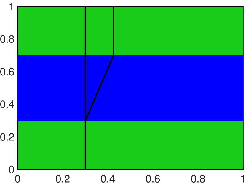
(a)

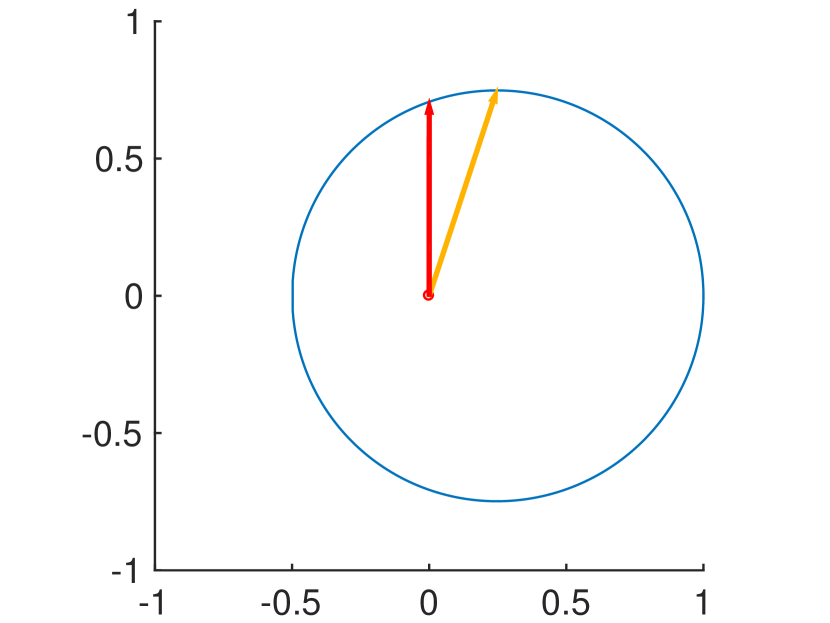
(b)

Figure 2: Optimal versus gradient path planning in subfigure (a). Corresponding velocity profile while “in the river” in subfigure (b).

We note that the parameter values used in [40] and subsequent publications seem highly unrealistic despite the experimental data used for calibration in [60]. For instance, consider two crowds with densities $\rho^{\textsc{a}}=\rho^{\textsc{b}}=1$ person per square meter. For convenience, we will define $\xi=f(1,0)-f(1,\pi)=1-e^{-2\beta}$, which gives the speed reduction resulting from these crowds moving in opposite directions rather than in unison. At $\beta=0.019$, if these crowds move in opposite directions, they are only slowed down by $\xi\approx 4.7\%$ of the full speed achievable when they move in unison. To provide some perspective, the classical estimate by Navin and Wheeler [50] used to calibrate many traffic engineering models yields a significantly higher $\beta=0.078.$ For our example, with $\rho^{\textsc{a}}=\rho^{\textsc{b}}=1$, this corresponds to a slow down of $\xi\approx 14.5\%$ relative to moving in unison. Even this last estimate appears rather conservative: anyone who has ever tried to catch a subway train during rush hour would attest that a speed reduction of $\xi\in[30\%,50\%]$ (corresponding to $\beta\in[0.178,0.347]$) would be much closer to their experience.

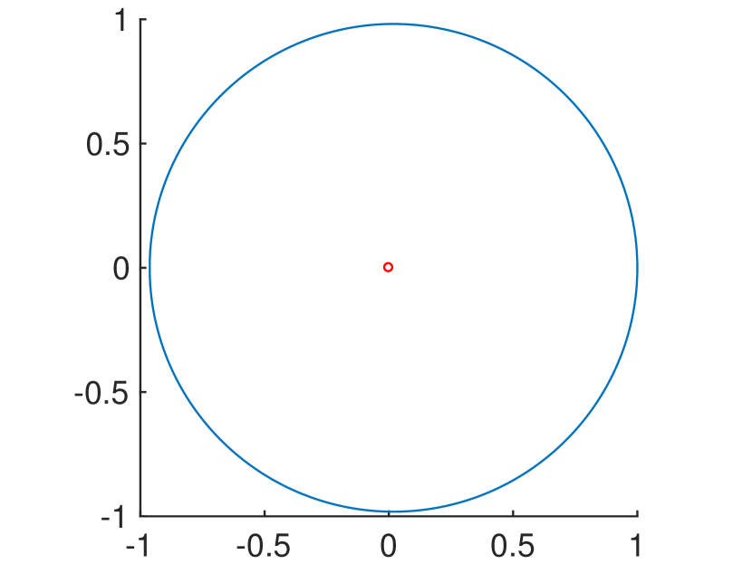
(a) $\beta=0.019$, $\bar{\rho}=1$
Convex velocity profile

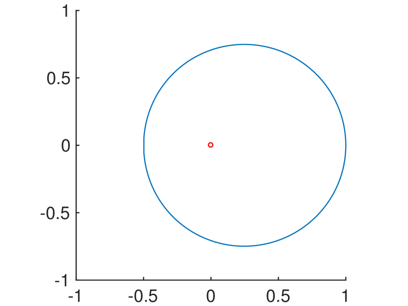
(b) $\beta=0.347$, $\bar{\rho}=1$
Convex velocity profile

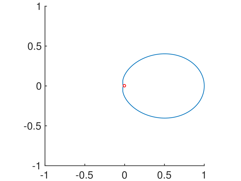
(c) $\beta=0.347$, $\bar{\rho}=2.4$
Non-convex velocity profile

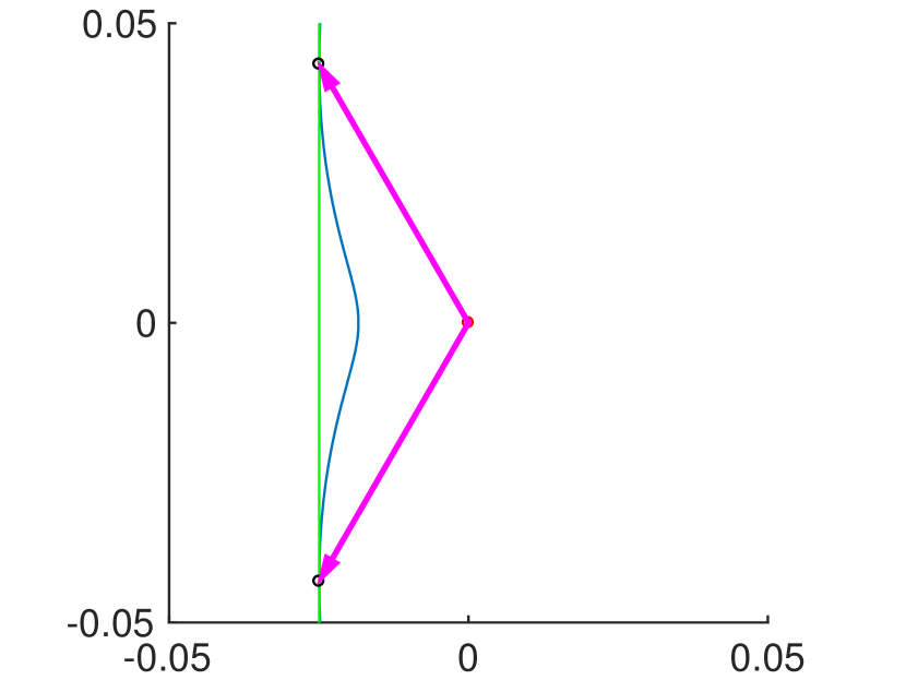
(d) Zoomed version of $\beta=0.347$, $\bar{\rho}=2.4$ to show non-convexity

Figure 3: Anisotropic velocity profiles for Crowd A at various parameter values. We assume $\mbox{\boldmath${u}$}^{\textsc{b}}_{*}=(1,0).$

For high enough values of $\rho^{\textsc{b}}$ or $\beta$, the velocity profile of crowd A can actually become non-convex. This scenario is highlighted in Figure 3(d). If a pedestrian tries to maximize the component of $\mbox{\boldmath${u}$}^{\textsc{a}}$ in the $-x$ direction, then both choices of $\mbox{\boldmath${u}$}^{\textsc{a}}$ denoted by the magenta arrows are optimal.

When looking at the velocity profile $\mathcal{V}$, we are concerned with only the smoothness and convexity of the profile, and not the scaling. Thus we need only look at the “disagreement penalty” factor $f(\rho^{\textsc{b}},\psi)$. Assuming that $\rho^{\textsc{b}}$ is fixed, we will further refer to it as $f(\psi)$ to simplify the notation. For a fixed $x$, we only need to check that the polar curve $\textbf{f}(\psi)=(f(\psi)\cos(\psi),f(\psi)\sin(\psi))$ is strictly convex, where $\psi$ is the angle between $\mbox{\boldmath${u}$}^{\textsc{a}}$ and $\mbox{\boldmath${u}$}^{\textsc{b}}$. If we consider its tangent vector $\textbf{T}(\psi)=\dot{\textbf{f}}(\psi)$, we can then write the derivative of the tangent vector as $\textbf{T}^{\prime}(\psi)=k(\psi)\textbf{N}(\psi)$, where $k$ is the curvature, and N is the unit normal vector. The sufficient condition for strict convexity is that $\textbf{T}(\psi)\times\textbf{N}(\psi)$ does not change sign. This reduces to a simple condition on $f$ and its derivatives:

$$f(\psi)^{2}+2f^{\prime}(\psi)^{2}-f(\psi)f^{\prime\prime}(\psi)>0,\quad\forall\psi$$ (3.10)

For the particular model (3.8), this condition simplifies to:

$$1+\beta\bar{\rho}^{2}\cos(\psi)+\beta\bar{\rho}^{2}\sin^{2}(\psi)>0.$$

We see that the left hand side is minimized when $\psi=\pi$. The sufficient condition for strict convexity then becomes

$$\beta\bar{\rho}^{2}<1.$$

At the parameter values used in [40], we see that we only lose strict convexity at densities exceeding $\bar{\rho}\approx 7.25$ people per square meter – a threshold which is too high to be relevant in practice. However, as discussed previously, their value of $\beta$ is rather small and with $\beta=0.078$ (consistent with Navin and Wheeler’s data [50]), we instead get that we can lose strict convexity when the density of either crowd exceeds a more physically relevant threshold of $\bar{\rho}=\sqrt{1/0.078}\approx 3.57.$

We summarize the results of using different values of $\beta$ in Table 1. The first two columns are for $\beta$ values consistent with Wong et al. [60] and Navin et al. [50] respectively. The third and fourth columns correspond to a slowdown of $\xi=0.3$ and $0.5$ respectively. In each case we list the critical density $\hat{\rho}$ at which the velocity profile loses strict convexity. We note that different “disagreement penalty factors” can be studied similarly. For example, a model considered in [26] is based on using $\bar{\rho}$ rather than $\bar{\rho}^{2}$; i.e.,

$$f(\bar{\rho},\psi)=e^{-\beta\left(1-\cos\psi\right)\bar{\rho}},$$ (3.11)

with the advantage that it scales more consistently for pairwise interactions of multiple crowds. The critical $\hat{\rho}$ values for this alternative model are reported in the last row of Table 1.

Table 1: Critical densities for two disagreement penalty models and various $\beta$ values.

$\beta$ 0.019 0.078 0.178 0.347 $\xi$ 0.037 0.144 0.3 0.5 critical density $\hat{\rho}$ for the $\beta\bar{\rho}^{2}$ model 7.25 3.58 2.37 1.70 critical density $\hat{\rho}$ for the $\beta\bar{\rho}$ model 52.6 12.8 5.62 2.88

3.2 Intra-crowd anisotropy.

Up until now we have only discussed models with localized interactions of pedestrians. But it is often reasonable to let the velocity $\mbox{\boldmath${V}$}(\boldsymbol{x},t)$ depend on values of $\rho(\cdot,t)$ in some region containing $\boldsymbol{x}$, rather than on a local $\rho(\boldsymbol{x},t)$ only. For multiple crowds, such non-local models present additional analytic challenges even if the direction field is specified in advance instead of chosen by individual pedestrians [16]. If individual choices are also included, non-local interactions give rise to anisotropy. In this section we show that this anisotropy may result in model inconsistency even for a single crowd.

In the paper by Cristiani, Priuli, and Tosin [19], the velocity is no longer chosen directly. Instead, it is the sum of a chosen behavioral velocity $\boldsymbol{u}\in S^{1}$, and an interaction velocity perturbation $\mbox{\boldmath${w}$}_{i}$ that is determined based on the density of pedestrians inside some sensory region $S(\boldsymbol{x},\boldsymbol{u})$. This sensory region is usually modeled by a sector (of angle $\alpha$ and radius $R$) centered at $\boldsymbol{x}$ and with the orientation determined by $\boldsymbol{u}$; see Figure 4. The key idea is that each pedestrian is only influenced by others roughly ahead of her, and not the ones behind. The model developed in [19] defines the interaction velocity $\mbox{\boldmath${w}$}_{i}$ as follows:

$$\mbox{\boldmath${w}$}_{i}=\int_{S(\boldsymbol{x},\boldsymbol{u})\cap\Omega}\mathcal{F}(\mbox{\boldmath${y}$}-\boldsymbol{x})\rho(t,\boldsymbol{x})\,d\mbox{\boldmath${y}$};\qquad\qquad\mathcal{F}(\boldsymbol{r})=\begin{cases}\frac{-F\boldsymbol{r}}{|\boldsymbol{r}|^{2}},&|\boldsymbol{r}|>\frac{1}{C},\\ \frac{-FC\boldsymbol{r}}{|\boldsymbol{r}|},&|\boldsymbol{r}|\leq\frac{1}{C},\end{cases}$$ (3.12)

where $F$ and $C$ are positive constants, with the latter functioning as a “cutoff”. Since the interaction velocity perturbation has a non-local dependence on the current $\rho$, it would be accurate to denote it $\mbox{\boldmath${w}$}_{i}\left[\rho(\cdot,t)\right](\boldsymbol{x},\boldsymbol{u})$, but we will at times abbreviate this as $\mbox{\boldmath${w}$}_{i}(\boldsymbol{x},\boldsymbol{u})$ or even $\mbox{\boldmath${w}$}_{i}$. The overall velocity is

$$\mbox{\boldmath${v}$}\left[\rho(\cdot,t)\right](\boldsymbol{x},\boldsymbol{u})\;=\;\boldsymbol{u}\,+\,\mbox{\boldmath${w}$}_{i}\left[\rho(\cdot,t)\right](\boldsymbol{x},\boldsymbol{u}),$$ (3.13)

which is a version of formula (2.3). Modulo this change from $\mbox{\boldmath${v}$}\left(\rho(\boldsymbol{x},t),\boldsymbol{u}\right)$ to $\mbox{\boldmath${v}$}\left[\rho(\cdot,t)\right](\boldsymbol{x},\boldsymbol{u})$, the functions $\rho$ and $\varphi$ satisfy the same system of PDEs (2.5).

Figure 4: An example of sensory region $S(\boldsymbol{x},\boldsymbol{u})$ for intra-crowd anisotropy.

We will now investigate the convexity of the velocity profiles for the case of intra-crowd anisotropy. Since this model depends non-locally on the density, we will only analyze this under some assumptions on the density function.

3.2.1 Linear Density.

First, let us consider the case of a density distribution that is linear in $\boldsymbol{x}$ at some fixed time $t$. WLOG we may assume that this density distribution is of the form:

$$\rho(x,y)=\rho_{0}+\rho_{x}x$$

In this case, we can evaluate the integral found in (3.12), which is done in Appendix A.

We note that for very high densities, the velocity profile may not actually contain the origin, as the interaction velocity can dominate the behavioral velocity. We show in Appendix B that as long as the density is linear in $\boldsymbol{x}$ and the velocity profile contains the origin, then we have convexity for all $\alpha$ such that $\alpha>3\sin(\alpha)$. This condition is satisfied for all $\alpha>\approx 130.57^{\circ}$, including the value of $\alpha=170^{\circ}$ used by Cristiani et al [19]. Otherwise, it may be possible to find a linear density function, and values for the parameters such that the velocity profile will not remain convex. For example, consider the case of $\alpha=20^{\circ},F=1,R=1$, $\rho_{0}=2$, and $\rho_{x}=-3/2$. A plot of this velocity profile can be found in Figure 5(a).

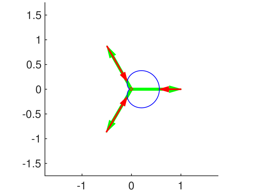
(a)

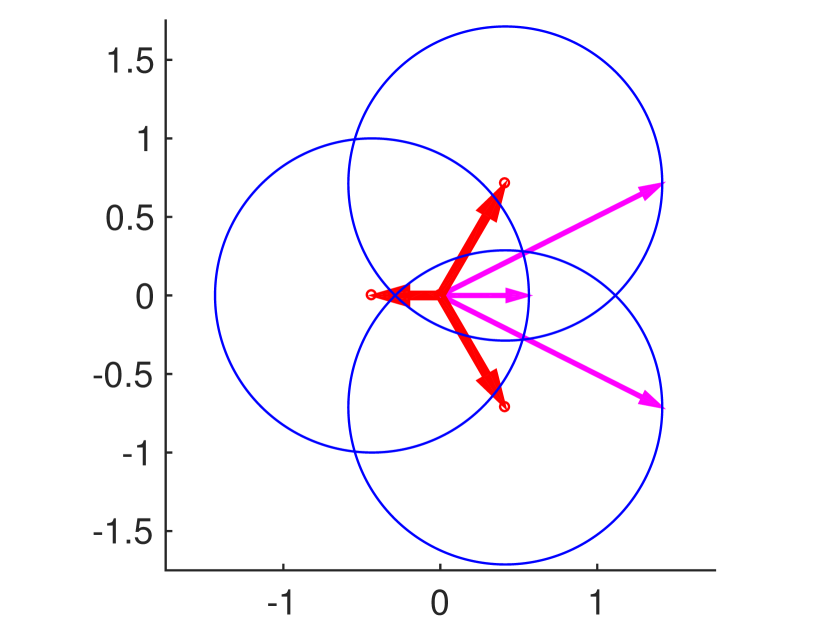
(b)

Figure 5: Left: Non-convex velocity profile for intra-crowd anisotropy and linear density with $\alpha=20^{\circ},F=1,R=1,\rho_{0}=2,\rho_{x}=-3/2$ on the left. Right: three “shifted circle” versions corresponding to different/fixed $\mbox{\boldmath${w}$}_{i}$ choices. Magenta arrows show the resulting velocity corresponding to $\boldsymbol{u}=(1,0)$ in each profile. One of them coincides with the correct resulting velocity in subfigure (a).

This linear density example is also good for illustrating another (general) pitfall in anisotropic modeling. In [19] the dynamics are given in the form:

$$\mbox{\boldmath${y}$}^{\prime}(t)=\boldsymbol{u}(t)+\mbox{\boldmath${w}$}_{i}[\rho(\tau,\cdot)](t)$$

However, this misleadingly suggests that $\mbox{\boldmath${w}$}_{i}$ is independent of the choice of $\boldsymbol{u}$. To illustrate this point, we show the correctly computed velocity profile in Figure 5(a) with three different versions of $\boldsymbol{u}$ in green and the corresponding $\mbox{\boldmath${w}$}_{i}$ vectors in red. Choosing any one of these $\mbox{\boldmath${w}$}_{i}$’s to be used for all $\boldsymbol{u}$ directions will yield a “shifted circle” velocity profile with very different resulting velocities; see Figure 5(b). Moreover, it is not clear which of these shifts would be a reasonable choice. This limits the validity of the simplified equation proposed in [19]

$$|\nabla\varphi|\,-\,\nabla\varphi\cdot\mbox{\boldmath${w}$}_{i}[\rho(\tau,\cdot)]\;=\;1$$

to radially symmetric sensing regions (i.e., with $\alpha=360^{\circ}$ only). Based on personal communications with the authors, the actual numerical tests in [19] have used a correct semi-Lagrangian discretization of the general HJB equation (2.5b).

3.2.2 Piecewise Constant Density.

We also considered piecewise constant density functions of the form:

$$\rho(x,y)=\begin{cases}\rho_{1},&x>0\\ \rho_{2},&x\leq 0\end{cases}$$

Here we find that both convexity and smoothness can also fail at $x=0$ for some parameter values, see the examples in Figure 6.

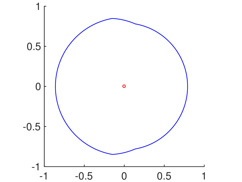
(a)

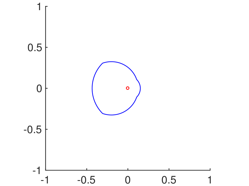
(b)

Figure 6: Non-convex velocity profiles for discontinuous density: $F=0.4$, $R=1$, $\rho_{1}=1.5$, $\rho_{2}=1$, $\alpha=20^{\circ}$ in (A) and the same except for $\alpha=90^{\circ}$ in (B).

4 Nash equilibria.

Returning to the problem of two-crowd interactions with $\rho=(\rho^{\textsc{a}},\rho^{\textsc{b}}),$ let us consider a speed function of the form:

$$v^{\textsc{a}}(\rho,\mbox{\boldmath${u}$}^{\textsc{a}})=f(\rho^{\textsc{b}},\psi)$$

with the corresponding velocity

$$\mbox{\boldmath${v}$}^{\textsc{a}}(\boldsymbol{x},\mbox{\boldmath${u}$}^{\textsc{a}})=\mbox{\boldmath${u}$}^{\textsc{a}}f(\rho^{\textsc{b}}(\boldsymbol{x}),\psi)$$

where $\mbox{\boldmath${u}$}^{\textsc{a}}$ and $\mbox{\boldmath${u}$}^{\textsc{b}}$ are the directions of motion of each crowd and $\psi$ is the angle between them.

In this case, the decision-making of the two crowds is modeled as a non-zero-sum game. We then look for a solution to the following coupled system of Hamilton-Jacobi-Isaacs (HJI) equations:

$$\max_{\mbox{\boldmath${u}$}^{\textsc{a}}\in S^{1}}\Bigl{\{}(\nabla\varphi^{\textsc{a}}(\boldsymbol{x})\cdot(-\mbox{\boldmath${u}$}^{\textsc{a}})v^{\textsc{a}}(\rho^{\textsc{a}}(\boldsymbol{x}),\mbox{\boldmath${u}$}^{\textsc{a}},\mbox{\boldmath${u}$}^{\textsc{b}})\Bigr{\}}=1$$ (4.14)

$$\max_{\mbox{\boldmath${u}$}^{\textsc{b}}\in S^{1}}\Bigl{\{}(\nabla\varphi^{\textsc{b}}(\boldsymbol{x})\cdot(-\mbox{\boldmath${u}$}^{\textsc{b}})v^{\textsc{b}}(\rho^{\textsc{b}}(\boldsymbol{x}),\mbox{\boldmath${u}$}^{\textsc{b}},\mbox{\boldmath${u}$}^{\textsc{a}})\Bigr{\}}=1$$ (4.15)

This notation is slightly misleading: each of the two PDEs involves maximizing in only one variable ($\mbox{\boldmath${u}$}^{\textsc{a}}$ or $\mbox{\boldmath${u}$}^{\textsc{b}}$), with the other one participating as a parameter. Both maximizations are assumed to be performed simultaneously, yielding the optimal pair of direction fields $(\mbox{\boldmath${u}$}^{\textsc{a}}_{*},\mbox{\boldmath${u}$}^{\textsc{b}}_{*}).$ A different pair of PDEs could be obtained by assuming that one of the crowds has an advantage of selecting its direction second (once the other crowd’s direction is already known). In general, the solution might change depending on which crowd we select to “go first”. This feature is disconcerting from a modeling perspective since the notion of “going first” is harder to motivate when the replanning is done continuously in time (with changing densities $\rho^{\textsc{a}}$ and $\rho^{\textsc{b}}$). So, it is desirable to guarantee that the order of decision making is irrelevant, making the system (4.14, 4.15) meaningful as written above. The sufficient condition for this is the uniqueness of the two-player Nash equilibrium (NE), a concept which we review below for general games.

We assume that player $A$ chooses strategies $a\in\mathcal{A}$ to maximize $J^{\textsc{a}}(a,b)$ and player $B$ chooses strategies $b\in\mathcal{B}$ to maximize $J^{\textsc{b}}(a,b)$. In the non-zero-sum setting (when $J^{\textsc{a}}\neq-J^{\textsc{b}}$) the well-posedness of the game is non-trivial even when $\mathcal{A}$ and $\mathcal{B}$ are discrete sets. NE is defined as a pair of strategies $(a_{*},b_{*})\in\mathcal{A}\times\mathcal{B}$ such that there is never an incentive to change unilaterally. More precisely, $(a_{*},b_{*})$ is said to be NE if both of the following hold:

$$J^{\textsc{a}}(a_{*},b_{*})\geq J^{\textsc{a}}(a,b_{*}),\quad\forall a\in\mathcal{A},$$

$$J^{\textsc{b}}(a_{*},b_{*})\geq J^{\textsc{b}}(a_{*},b),\quad\forall b\in\mathcal{B}.$$

If the game has a unique NE, then we can always assume that both players make their decisions simultaneously – if both players are rational, there is no longer any advantage to “go second.”

The existence of NE for infinite continuous games has been proved under some very general assumptions, at least in the class of mixed policies [23]. For zero-sum-games, the possible non-uniqueness is not a major issue and requires no coordination between the players. If both $(a_{*},b_{*})$ and $(a_{\sharp},b_{\sharp})$ are NE, then so are $(a_{*},b_{\sharp})$ and $(a_{\sharp},b_{*})$; moreover, $J^{\textsc{a}}$ will have the same value for each of these pairs (and $J^{\textsc{b}}=-J^{\textsc{a}}$). So, who goes first and which NE they aim for still does not matter. However, none of this holds in the case of non-zero-sum games. In section 4.2 we will show examples where the value of multiple NE is different, players disagree about their relative merits, and choosing simultaneously without coordination can easily lead to a non-Nash outcome.

In the case of zero-sum HJI games, the notions of “upper value” and “lower value” are used to capture what happens when one of the players goes first. A separate “Isaacs criterion” on the Hamiltonian ensures that these two values are always equal, enabling simultaneous decision-making by the players. Additional mild technical conditions guarantee that a NE exists among pure strategies, making it unnecessary to consider any relaxed/“chattering” controls [4]. A simple modification of this argument yields the existence of a pure-strategy NE in (4.14, 4.15) provided both velocity profiles are strictly convex. However, to claim that this non-zero-sum system has a well-defined value, we will also need to know that this NE is unique.

We will focus on a fixed $\boldsymbol{x}\in\Omega$, assuming that $\rho$’s and $\varphi$’s are known for both crowds and writing $\textbf{p}=\nabla\varphi_{\textsc{a}}(\textbf{x}),\;\textbf{q}=\nabla\varphi_{\textsc{b}}(\textbf{x})$ to simplify the notation:

$$\max_{\mbox{\boldmath${u}$}^{\textsc{a}}\in S^{1}}\Bigl{\{}\mbox{\boldmath${p}$}\cdot(-\mbox{\boldmath${u}$}^{\textsc{a}})\,v^{\textsc{a}}\left(\rho^{\textsc{b}}(\boldsymbol{x}),\mbox{\boldmath${u}$}^{\textsc{a}},\mbox{\boldmath${u}$}^{\textsc{b}}\right)\Bigr{\}}=1;\hfill\qquad\qquad\max_{\mbox{\boldmath${u}$}^{\textsc{b}}\in S^{1}}\Bigl{\{}\mbox{\boldmath${q}$}\cdot(-\mbox{\boldmath${u}$}^{\textsc{b}})\,v^{\textsc{b}}\left(\rho^{\textsc{a}}(\boldsymbol{x}),\mbox{\boldmath${u}$}^{\textsc{a}},\mbox{\boldmath${u}$}^{\textsc{b}}\right)\Bigr{\}}=1.$$

Furthermore, to focus on the geometric aspects we will use $\Delta$ to denote the angle between ${p}$ and ${q}$, $\psi$ for the angle between $\mbox{\boldmath${u}$}^{\textsc{a}}$ and $\mbox{\boldmath${u}$}^{\textsc{b}}$, and $(a,b)$ for the angles that $\mbox{\boldmath${u}$}^{\textsc{a}}$ and $\mbox{\boldmath${u}$}^{\textsc{b}}$ make with $(-\mbox{\boldmath${p}$})$ and $(-\mbox{\boldmath${q}$})$ respectively.

From the definition (3.9), we note that the anisotropic speeds $v^{\textsc{a}}$ and $v^{\textsc{b}}$ have a common isotropic factor which does not affect the choice of optimal direction. Denote $f^{\textsc{a}}(\psi)=f(\rho^{\textsc{b}},\psi)$, $f^{\textsc{b}}(\psi)=f(\rho^{\textsc{a}},\psi)$, recall that $\psi=a-b+\Delta$, and our new task is to show the uniqueness of the NE for all $(\mbox{\boldmath${p}$},\mbox{\boldmath${q}$})$ in the equivalent game

$$\max_{a\in[0,2\pi]}\Bigl{\{}\cos(a)f^{\textsc{a}}(a-b+\Delta)\Bigr{\}}=1,\hfill\qquad\qquad\max_{b\in[0,2\pi]}\Bigl{\{}\cos(b)f^{\textsc{b}}(a-b+\Delta)\Bigr{\}}=1.$$ (4.16)

We will assume that the velocity profiles for both crowds are smooth and strictly convex. The strict convexity ensures that the $\mathop{\mathrm{argmax}}_{a\in[0,2\pi]}$ is unique for every $b$, making the “best reply” map $\Phi^{\textsc{a}}(b)$ well-defined. Since $f^{\textsc{a}}$ is smooth, the first-order optimality condition

$$0\;=\;\frac{d}{da}\Bigl{[}\cos(a)f^{\textsc{a}}(a-b+\Delta)\Bigr{]}=-\sin(a)f^{\textsc{a}}(a-b+\Delta)+\cos(a)\frac{\partial}{\partial a}\bigl{[}f^{\textsc{a}}(a-b+\Delta)\bigr{]}$$ (4.17)

should hold for $a=\Phi^{\textsc{a}}(b).$ If we denote the right hand side as $g(a,b)$, then

$$\frac{\partial g}{\partial a}\,=\,-\cos(a)f^{\textsc{a}}(\psi)-2\sin(a)\frac{df^{\textsc{a}}}{d\psi}+\cos(a)\frac{d^{2}f^{\textsc{a}}}{d\psi^{2}};\qquad\frac{\partial g}{\partial b}\,=\,-\sin(a)\frac{df^{\textsc{a}}}{d\psi}+\cos(a)\frac{d^{2}f^{\textsc{a}}}{d\psi^{2}}.$$

Noting that (4.17) implies $\sin(a)=\cos(a)\frac{\frac{df^{\textsc{a}}}{d\psi}}{f^{\textsc{a}}(\psi)},$ we can now simplify the derivative

$$\frac{d\Phi^{\textsc{a}}}{db}\,=\,\frac{-g_{b}}{g_{a}}\,=\,\frac{-\left(\frac{df^{\textsc{a}}}{d\psi}\right)^{2}+f^{\textsc{a}}(\psi)\frac{d^{2}f^{\textsc{a}}}{d\psi^{2}}}{-f^{\textsc{a}}(\psi)^{2}-2\left(\frac{df^{\textsc{a}}}{d\psi}\right)^{2}+f^{\textsc{a}}(\psi)\frac{d^{2}f^{\textsc{a}}}{d\psi^{2}}}.$$ (4.18)

A similar derivation can be repeated for the other crowd’s best reply $\Phi^{\textsc{b}}(a)$. If we show that the map $a\mapsto\Phi^{\textsc{a}}(\Phi^{\textsc{b}}(a))$ is a contraction mapping, the existence and uniqueness of NE becomes a simple consequence of the Banach fixed-point theorem.

Thus, it is sufficient to show that the derivative is bounded by 1, i.e.

$$\left|\frac{d}{da}\Bigl{[}\Phi^{\textsc{a}}(\Phi^{\textsc{b}}(a))\Bigr{]}\right|<1,\qquad\forall a\in[0,2\pi]$$

It is generally easier to check the slightly stronger condition following from the Chain Rule that

$$\left|\frac{d\Phi^{\textsc{a}}}{db}\right|\left|\frac{d\Phi^{\textsc{b}}}{da}\right|<1,\qquad\forall(a,b)\in[0,2\pi]\times[0,2\pi]$$

where the derivatives of the best reply maps can be found in Equation (4.18).

4.1 NE in intercrowd models.

In [40], they assume a speed function for crowd $A$ of the form:

$$v^{\textsc{a}}(\psi)=v_{0}e^{-\alpha(\left(\rho^{\textsc{a}}\right)^{2}+\left(\rho^{\textsc{b}}\right)^{2})}e^{-\beta\left(\rho^{\textsc{b}}\right)^{2}(1-\cos(\psi))}$$

where $\rho$ is the density of the other crowd. (Crowd $B$’s speed function is defined analogously.) Since we are interested only in the shape (rather than scaling) of the velocity profile, we shall just use:

$$f^{\textsc{a}}(\psi)=e^{-\beta\left(\rho^{\textsc{b}}\right)^{2}(1-\cos(\psi))}$$

as it is simpler to work with. For ease of notation, we shall also drop the superscripts on $\rho.$ We calculate that

$$\frac{df^{\textsc{a}}}{d\psi}=-\beta\rho^{2}\sin(\psi)e^{-\beta\rho^{2}(1-\cos(\psi))},$$

$$\frac{d^{2}f^{\textsc{a}}}{d\psi^{2}}=\beta^{2}\rho^{4}\sin(\psi)^{2}e^{-\beta\rho^{2}(1-\cos(\psi))}-\beta\rho^{2}\cos(\psi)e^{-\beta\rho^{2}(1-\cos(\psi))}.$$

Plugging these into Equation (4.18), we obtain

$$\left|\frac{d\Phi^{\textsc{a}}}{db}\right|\,=\,\left|\frac{\beta\rho^{2}\cos(\psi)}{\beta\rho^{2}\cos(\psi)+\beta^{2}\rho^{4}\sin^{2}(\psi)+1}\right|.$$ (4.19)

We see that the denominator is a quadratic polynomial in $\cos(\psi)$. If we assume the necessary and sufficient condition for strict convexity that $\beta\rho^{2}<1$, then it follows that the absolute value of this polynomial reaches a minimum of $1-\beta\rho^{2}$ at $\psi=\pi$. Similarly, the numerator is maximized in absolute value at $\psi=\pi$, so we see that the worst case scenario is that of $\psi=\pi$, where the derivative is bounded by:

$$\left|\frac{d\Phi^{\textsc{a}}}{db}\right|\,<\frac{\beta(\rho^{\textsc{b}})^{2}}{1-\beta(\rho^{\textsc{b}})^{2}}.$$ (4.20)

The same process works with the crowds switched. So $\Phi^{\textsc{a}}(\Phi^{\textsc{b}}(a))$ is a contraction mapping (and NE is unique) whenever

$$\frac{\beta(\rho^{\textsc{b}})^{2}}{1-\beta(\rho^{\textsc{b}})^{2}}\frac{\beta(\rho^{\textsc{a}})^{2}}{1-\beta(\rho^{\textsc{a}})^{2}}<1\qquad\text{or, equivalently,}\qquad\beta(\rho^{\textsc{a}})^{2}+\beta(\rho^{\textsc{b}})^{2}<1.$$ (4.21)

The models in [40] assume a value of $\beta=0.019$, which means that our condition for guaranteeing the uniqueness of NE becomes:

$$(\rho^{\textsc{a}})^{2}+(\rho^{\textsc{b}})^{2}<\frac{1}{\beta}\approx 52.632;$$ (4.22)

i.e., NE will be unique for all physically relevant crowd densities. However, this criterion becomes much more restrictive for higher (more realistic) values of $\beta$. For example, at $\beta=0.347$, the condition is now $(\rho^{\textsc{a}})^{2}+(\rho^{\textsc{b}})^{2}<2.881$, which is definitely violated when $\rho^{\textsc{a}}+\rho^{\textsc{b}}\geq 2.41$ even if $\max\left(\rho^{\textsc{a}},\rho^{\textsc{b}}\right)\leq\hat{\rho}\approx 1.7$ and the velocity profiles are convex; see also Table 1 and Figure 7. Similarly, for the alternative disagreement penalty model based on $(\beta\bar{\rho})$, the corresponding sufficient condition for the uniqueness of NE is $\rho^{\textsc{a}}+\rho^{\textsc{b}}<\frac{1}{\beta}=\hat{\rho}.$ For $\beta=0.347$, this means that the uniqueness might be lost when the total density of both crowds exceeds $2.881$.

Our numerical experiments show that the above conditions are actually sharp: all densities from Region 2 in Figure 7 seem to yield multiple NE. However, the experiments also show that this only happens when ${p}$ and $(-\mbox{\boldmath${q}$})$ are sufficiently close; e.g., at $\beta=0.5$ in the $(\beta\bar{\rho}^{2})$ model and $\rho^{\textsc{a}}=\rho^{\textsc{b}}=1.2$, we only observe multiple NE when the angle between ${p}$ and ${q}$ is greater than 171 degrees.

$\begin{array}[]{cc}\leavevmode\hbox to110.17pt{\vbox to113.96pt{\text{[drawing]}}}&\leavevmode\hbox to110.17pt{\vbox to113.96pt{\text{[drawing]}}}\\ (a)&(b)\end{array}$

Figure 7: Critical density regions for the $\beta(\bar{\rho})^{2}$ model (subfigure a) and for the $\beta\bar{\rho}$ model (subfigure b). Provably unique NE in Region 1; multiple NE observed in Region 2; non-convex velocity profiles in Region 3.

4.2 NE Examples.

Example 1

Here we consider an example with $\mbox{\boldmath${p}$}=(1,0)$ and $\mbox{\boldmath${q}$}=(-1,0)$, with $\beta=0.347$, $\rho^{\textsc{a}}=1.68$, and $\rho^{\textsc{b}}=0.72$ Numerically, we find three NEs at:

$$\left(\begin{array}[]{c}a\\ b\end{array}\right)=\left(\begin{array}[]{c}3.1416\\ 0\end{array}\right),\left(\begin{array}[]{c}3.0366\\ 0.5208\end{array}\right),\text{ and }\left(\begin{array}[]{c}3.2466\\ 5.7623\end{array}\right).$$

A plot of $-\mbox{\boldmath${p}$},-\mbox{\boldmath${q}$}$ and the velocity profiles for each NE can be found in Figure 8. The orange arrow is $-\mbox{\boldmath${p}$}$ and the green arrow is $-\mbox{\boldmath${q}$}$. The velocity profile and choice of direction for crowd $A$ are plotted in red, while the same is plotted in blue for crowd $B$.

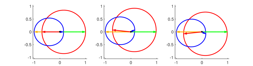
Figure 8: $-\mbox{\boldmath${p}$}$,$-\mbox{\boldmath${q}$}$, and velocity profiles for each NE in Example $1$.

Example 1 is also summarized below in bimatrix form. Both crowds try to maximize their respective outcomes based on (4.16); each entry contains the payoff for the “row player” (crowd A) and the “column player” (crowd B). Of course, both of them have infinitely many options, but we include only those corresponding to Figure 8. The NE outcomes are on the diagonal, and their payoffs are different; so, the “value” of this game is not well-defined. Moreover, since the crowds do not coordinate, they cannot know which NE control the other player will choose and this lack of coordination will frequently result in non-Nash (off-diagonal) outcomes.

Nash Equilibria payoffs for Example 1

	0	0.5208	5.7623
3.1416	0.698, 0.141	0.715, 0.139	0.715, 0.139
3.0366	0.695, 0.142	0.718, 0.147	0.705, 0.133
3.2466	0.695, 0.142	0.705, 0.133	0.718, 0.147

Example 2

Now for an example where $\mbox{\boldmath${p}$}\not=-\mbox{\boldmath${q}$}$. Here we take $\mbox{\boldmath${p}$}=(\cos(\pi/20),\sin(\pi/20))$ and $\mbox{\boldmath${q}$}=(\cos(39\pi/40),\sin(39\pi/40))$, with $\beta=0.347$, $\rho^{\textsc{a}}=1.68$, and $\rho^{\textsc{b}}=1.68$. Numerically, we now find two NEs, this time at:

$$\left(\begin{array}[]{c}a\\ b\end{array}\right)=\left(\begin{array}[]{c}2.5470\\ 0.6732\end{array}\right),\text{ and }\left(\begin{array}[]{c}4.0641\\ 5.4393\end{array}\right).$$

A plot of $-\mbox{\boldmath${p}$},-\mbox{\boldmath${q}$}$ and the velocity profiles for each NE can be found in Figure 9

Figure 9: $-\mbox{\boldmath${p}$}$,$-\mbox{\boldmath${q}$}$, and velocity profiles for each NE in Example $2$.

NE payoffs for Example 2

	0.6732	5.4393
2.5470	0.205, 0.205	0.106, 0.105
4.0641	0.105, 0.106	0.328, 0.328

From our numerical experiments, it seems that all cases with $\mbox{\boldmath${p}$}\not=-\mbox{\boldmath${q}$}$ and multiple NEs are qualitatively similar to Example 2. Since $\mbox{\boldmath${p}$}\not=-\mbox{\boldmath${q}$}$, we can think of $-\mbox{\boldmath${p}$}$ and $-\mbox{\boldmath${q}$}$ as splitting the plane into two sections, one where the angle between them is greater than $\pi$, and one where the angle is less than $\pi$. We always see two NEs, one in the section with angle greater than $\pi$, one in the other section. The NE on the side where the angle is less than $\pi$ then has higher payoffs for both crowds, dominating the other NE.

Example 3

In the previous examples, we showed that multiple NEs are possible even if the velocity profile is strictly convex and smooth. In this last example we aim to illustrate that a strictly convex but non-smooth velocity profile can result in infinitely many NEs. Let us consider a speed function with “disagreement penalty” of the form:

$$f(\bar{\rho},\psi)=e^{-C\bar{\rho}\left(\pi^{2}-(\text{mod}(\psi,2\pi)-\pi)^{2}\right)}.$$

The resulting velocity profiles form a strictly convex but non-smooth teardrop-like shape as seen in Figure 10. In the different subfigures of Figure 10, we have consistently chosen $C=0.1$ and $\rho^{\textsc{a}}=\rho^{\textsc{b}}=1$, keeping ${p}$ and ${q}$ symmetric relative to the $x$-axis. We explore how the NEs change as we decrease the angle $\theta$ between $(-\mbox{\boldmath${p}$})$ and $(-\mbox{\boldmath${q}$}),$ which are shown by the orange and green arrows respectively.

$\begin{array}[]{cccc}\includegraphics[width=108.405pt]{Figures/NonSmoothNash1.pdf}&\includegraphics[width=108.405pt]{Figures/NonSmoothNash2.pdf}&\includegraphics[width=108.405pt]{Figures/NonSmoothNash3.pdf}&\includegraphics[width=108.405pt]{Figures/NonSmoothNash4.pdf}\\ (a)&(b)&(c)&(d)\end{array}$

Figure 10: Example 3: NEs for non-smooth velocity profiles as $(-\mbox{\boldmath${p}$})$ in orange and $(-\mbox{\boldmath${q}$})$ in green move closer together. Subfigures $(c)$ and $(d)$ show a few of infinitely many NEs.

Figure 10a shows the case $\theta=2\pi/3$, with a unique NE, both crowds having distinct velocity profiles and different choices of optimal directions (shown in red and blue). As ${p}$ and ${q}$ move closer together, we still have a unique NE up until the critical angle $\theta_{c},$ when the velocity profiles of both crowds (and the respective optimal directions) coincide; see Figure 10b. A simple geometric argument shows that $\theta_{c}=\pi/2-\arctan(1/(2\pi C\bar{\rho})).$ For $\theta\in[0,\theta_{c}),$ the NE is no longer unique even though in each of them both velocity profiles coincide and both crowds choose the same “optimal” direction corresponding to the tip of the velocity profile. Note that only some of these NEs are Pareto optimal (the ones where the tip lies in between $(-\mbox{\boldmath${p}$})$ and $(-\mbox{\boldmath${q}$})$), and many others are not; see the full range of Nash-profiles in Figure 10c. It is worth noting that the case $\mbox{\boldmath${p}$}=\mbox{\boldmath${q}$}$ can also be viewed as one crowd artificially divided into two, whose goals/destinations are actually the same. In order for our model to remain consistent, we would hope that there is a unique NE corresponding to the optimal choice of direction for the isotropic (one-crowd) model. Figure 10d shows that this is actually not the case and we have infinitely many NEs even with $\theta=0.$ (However, only one of them, corresponding to the vertically symmetric velocity profile and the “isotropically optimal” direction of motion $\frac{-\mbox{\boldmath${p}$}}{|\mbox{\boldmath${p}$}|}$, is now Pareto-optimal). This suggests that the smoothness of the velocity profile is also a natural consistency condition even for the single crowd models.

5 Numerical Implementation and Experiments.

The fully coupled system (2.5) is typically discretized via explicit time-stepping: the current density $\rho$ is used to compute $\varphi$ in the current time slice, and the recovered $\boldsymbol{u}_{*}$ is then used to find $\rho$ in the next time-slice via (2.5a, 2.5d). In [31] this approach was used with WENO-based discretizations for both the conservation law and the isotropic Eikonal PDE. Our own simpler implementation relies on a Lax-Friedrichs scheme [46] for the hyperbolic conservation law (2.5a) and a first-order accurate semi-Lagrangian discretization of the HJB equation (2.5b).

Modeling the choice of optimal directions presents two main challenges. The first is a choice of suitable discretization for the anisotropic / static HJ PDEs, yielding a large system of coupled (discretized) equations in each time slice. The second is an efficient method for solving this discretized system. In the following discussion we primarily focus on the latter challenge and also emphasize the connection to our consistency criteria covered in previous sections. We will first discuss the numerical methods for a single HJB PDE (2.5b) in Section 5.1, followed by a discussion of numerics for two coupled HJI equations in Section 5.2, and two-crowd simulation results in Section 5.3.

5.1 Numerical solution of HJB for a single anisotropic crowd.

If $\rho$ is known and $t>0$ is fixed, then $\varphi$ is the viscosity solution of the Hamilton-Jacobi-Bellman equation (2.5b), and $\boldsymbol{u}_{*}$ can be recovered from (2.5c). In the special case of isotropic dynamics (i.e. when $\mbox{\boldmath${v}$}(\rho(\boldsymbol{x},t),\boldsymbol{u})=v(\rho(\boldsymbol{x},t))\boldsymbol{u}$ and $\boldsymbol{u}\in S^{1}$), this HJB PDE reduces to an Eikonal equation (2.6), for which many competing efficient algorithms have been developed in the last 20 years. Dijkstra-like (“Fast Marching”) methods [59, 53, 56] provide non-iterative solvers by dynamically recovering the correct ordering of discretized equations and solving them one at a time. These methods have been extended to meshes on manifolds [42, 52], higher-order accurate Eulerian [54, 1] and semi-Lagrangian discretizations [18], and more general anisotropic cases [55, 2, 49]. An alternative (“Fast Sweeping”) approach is based on alternating through a set of natural geometric orderings to speed up the convergence of Gauss-Seidel iterations [7, 64, 58, 41, 47, 62, 63, 6]. Each of these two approaches is particularly efficient on its own subset of problems. More recently, hybrid (two-scale) methods have been introduced in [13, 14] to combine the advantages of both marching and sweeping. These papers also include a review of several other “fast Eikonal solvers” (mirroring the logic of label-correcting algorithms on graphs) and their parallel implementations.

Our own simulations use Fast Sweeping – primarily because this approach is easier to extend to multi-crowd scenarios discussed in section 5.2.

In principle, the computational cost of solving (2.5b) in each time-slice can be further reduced by only computing $\varphi$ on the relevant subset of $\bar{\Omega}$. Such “causal domain restriction” techniques are reminiscent of the classical A* algorithm on graphs [27] and have been also extended to Eikonal equations; see [15] and references therein. In pedestrian flow modeling, similar ideas have been used to speed up the “dynamic floor field” computation in [28].

For the general/anisotropic version of the pedestrian direction field problem, it usually is not possible to write down the analytic expression for $\boldsymbol{u}_{*}$ even if $\nabla\varphi$ is already known. The HJB equation (2.5b) is then most naturally discretized in a semi-Lagrangian framework [21], with $\boldsymbol{u}_{*}$ recovered at each gridpoint through a numerical optimization over all $\boldsymbol{u}\in\mathcal{U}$.

This numerical optimization often presents a significant computational bottleneck, particularly so for non-local models, in which evaluating the velocity ${v}$ for any specific $\boldsymbol{u}$ is already expensive. We recall that in [19] the velocity is computed as the sum of a chosen velocity $\boldsymbol{u}$ and an interactional velocity $\mbox{\boldmath${w}$}_{i}$; see formula (3.13). Computing the value of $\mbox{\boldmath${w}$}_{i}$ requires calculating an integral over a sensory region $S(\boldsymbol{x},\boldsymbol{u})$ that changes with each choice of $\boldsymbol{u}$. However, if the density is approximately linear within the sensory region $S(\boldsymbol{x},\boldsymbol{u})$, our work in Appendix A shows how to evaluate this integral analytically, which could be used to speed up the numerics.

Aside from being computationally expensive, the numerical optimization to find $\boldsymbol{u}_{*}$ may “mask” some of the possible model inconsistencies: if the argmax in (2.5c) is not unique (e.g., when the velocity profile is not strictly convex), this can easily go unnoticed and the simulation results will become dependent on the specific implementation of optimization on $\mathcal{U}.$ To avoid these issues, it is important to verify the convexity of the speed profile either a priori or at run-time (based on the crowd densities observed in the simulation).

5.2 Implementation notes for two-crowd models.

In Section 4, we discussed uniqueness of Nash Equilibria for the system of coupled Hamilton-Jacobi-Isaacs PDEs (4.14) and (4.15). For numerical simulations, the semi-Lagrangian discretization of these PDEs on the grid results in a pair of coupled optimization problems at each gridpoint $(i,j)$:

$$\varphi^{\textsc{a}}_{ij}\;=\;\min_{\mbox{\boldmath${u}$}^{\textsc{a}}_{ij}\in S^{1}}G\left(\rho^{\textsc{a}}_{ij},\rho^{\textsc{b}}_{ij},\mbox{\boldmath${u}$}^{\textsc{b}}_{ij},N\varphi^{\textsc{a}}_{ij}\right),$$ (5.23)

$$\varphi^{\textsc{b}}_{ij}\;=\;\min_{\mbox{\boldmath${u}$}^{\textsc{b}}_{ij}\in S^{1}}G\left(\rho^{\textsc{a}}_{ij},\rho^{\textsc{b}}_{ij},\mbox{\boldmath${u}$}^{\textsc{a}}_{ij},N\varphi^{\textsc{b}}_{ij}\right),$$ (5.24)

where $N\varphi^{\textsc{a}}_{ij}$ refers to the values of $\varphi^{\textsc{a}}$ at the neighboring gridpoints to $(i,j)$. Ideally, we would like to know that the system (5.23-5.24) has a unique Nash Equilibrium regardless of values of $\rho^{\textsc{a}}_{ij},\rho^{\textsc{b}}_{ij},N\varphi^{\textsc{a}}_{ij},$ and $N\varphi^{\textsc{b}}_{ij}$ whenever the same is true for (4.14-4.15) regardless of the vectors $\nabla\varphi^{\textsc{a}}$ and $\nabla\varphi^{\textsc{b}}$. Our numerical experiments confirm this equivalence, but it has not been proven rigorously so far.

These coupled discretized equations have to be solved at every gridpoint. A natural approach for doing this is to mimic the structure of the “best reply” map in Section 4. If $\varphi$ for one of the crowds is assumed to be known, then $\varphi$ for the other crowd can be solved as in the one-crowd case (e.g., by Fast Sweeping; see Section 5.1). So, we can alternate through solving equations (5.23) and (5.24), freezing the current version of $\varphi^{\textsc{a}}$ and $\mbox{\boldmath${u}$}^{\textsc{a}}$ to recover $\varphi^{\textsc{b}}$ and $\mbox{\boldmath${u}$}^{\textsc{b}}$, which are then used to update $\varphi^{\textsc{a}}$ and $\mbox{\boldmath${u}$}^{\textsc{a}}$, and so on. When the (discretized) best reply map is a contraction, its fixed point is the unique Nash equilibrium and this iterative process converges to it. The examples in Section 5.3 show simulations of two crowds computed in this manner which exhibit qualitative behavior similar to real crowds. If we initialize the discretized best reply map with some initial choice of directions (e.g. from the previous time step), then the convergence of this map is proof that both crowds are in fact using Nash equilibrium strategies. However, this approach is not sufficient to guarantee that this Nash equilibrium is also unique, even if the simulation appears plausible from a phenomenological perspective.

A more careful approach is to iterate over the gridpoints in the outer loop, freezing $\left(N\varphi^{\textsc{a}}_{ij},N\varphi^{\textsc{b}}_{ij}\right)$ and updating $(\varphi^{\textsc{a}}_{ij},\varphi^{\textsc{b}}_{ij})$ simultaneously. We can discretize the control space $S^{1}$ (considering a fixed/finite number of directions of motion) and then find the Nash equilibria for the resulting finite bi-matrix game. One advantage is that we can directly verify the number of Nash equilibria, though it might also change as we refine the discretization of $S^{1}.$

Since the coupled system (4.14-4.15) has to be solved in every time-slice, it is desirable to speed up the above procedures as much as possible. One heuristic approach is based on updating the crowd direction fields by measuring the angle $\Psi$ between our currently chosen direction and the direction used by the other crowd in the previous time-slice. This idea (similar to the approach used in [40] and the subsequent papers) effectively decouples the PDEs, speeding up the numerics and side-stepping all Nash-equilibria issues. However, there is no proof that the resulting evolution of crowd densities is the same as one would recover from actually solving the coupled system (4.14-4.15).

5.3 Numerical Experiments with Two Crowds.

This subsection contains a few simulation results based on our implementation of the anisotropic two-crowd model found in [40], discussed previously in Sections 3.1 and 4.1. As a reminder, the corresponding speed functions are:

$$v^{\textsc{a}}\left(\rho^{\textsc{a}},\rho^{\textsc{b}},\mbox{\boldmath${u}$}^{\textsc{a}},\mbox{\boldmath${u}$}^{\textsc{b}}\right)=\bar{v}e^{-\alpha\left(\rho^{\textsc{a}}+\rho^{\textsc{b}}\right)^{2}}f(\rho^{\textsc{b}},\psi)\;\text{ and }\;v^{\textsc{b}}\left(\rho^{\textsc{a}},\rho^{\textsc{b}},\mbox{\boldmath${u}$}^{\textsc{a}},\mbox{\boldmath${u}$}^{\textsc{b}}\right)=\bar{v}e^{-\alpha\left(\rho^{\textsc{a}}+\rho^{\textsc{b}}\right)^{2}}f(\rho^{\textsc{a}},\psi)$$

where $f$ is given by:

$$f(\bar{\rho},\psi)=e^{-\beta\left(1-\cos\psi\right)\bar{\rho}^{2}}.$$

In all examples, we will use $\alpha=0.075$ and $\bar{v}=1$ meter/second on a $100$m by $100$m square domain $\Omega$. Our code also verifies that the models stay consistent throughout the simulations; i.e., the densities stay in Region 1 defined in Figure 7a.

Example 1: Difference in Direction Fields

This example is meant to highlight the difference between optimal and gradient path-planning. In Figure 11, crowds A and B are trying to reach exits on the South and North sides of the domain, respectively. The crowds are initially intermixed and their optimal direction fields (shown in blue) are different from the gradient fields of their respective value functions (shown in red). The red directions appear to indicate shorter paths toward the desired exits, but using them would be suboptimal since the corresponding “disagreement penalty” to the speeds would be higher. This can be interpreted as a more “organic” version of the example in Figure 2.

$\begin{array}[]{ccccc}\includegraphics[width=41.19443pt]{Figures/ColorBar.pdf}&\includegraphics[width=121.41306pt]{Figures/DiffDensityA.pdf}&\includegraphics[width=121.41306pt]{Figures/DiffDensityB.pdf}&\includegraphics[width=121.41306pt]{Figures/DiffDirectionsA.pdf}&\includegraphics[width=121.41306pt]{Figures/DiffDirectionsB.pdf}\\ &(a)&(b)&(c)&(d)\end{array}$

Figure 11: Two interacting crowds aiming for different exits on a domain with a single obstacle. Subfigures (a) and (b): contour plots of $\rho^{\textsc{a}}$ and $\rho^{\textsc{b}}$ at $t=1.5$ with the respective exits shown in black. Subfigures (c) and (d): their corresponding optimal direction fields (in blue) and gradient fields (in red). Computed for $\beta=0.347$ on a $100$x$100$ grid with timestep $\Delta t=0.5.$

Exmaple 2: Lane Formation

This example is meant to illustrate lane formation of two crowds in an intercrowd model based on [40]. Each crowd flows in from an entrance on the side of the domain (shown in dark gray), with Crowd $A$ flowing in from the left at a rate of 0.8 $\text{ped}\cdot m^{-1}\cdot s^{-1}$ and Crowd $B$ flowing in from the right at a rate of 0.4 $\text{ped}\cdot m^{-1}\cdot s^{-1}$. Each crowd then aims to reach a target on the opposite side of the domain (shown in black). As can be seen in Figure 12, both crowds form lanes to avoid each other. Since this is similar to behavior of real crowds, such phenomena are often used to argue for the validity of PDE models. It is worth noting that the lanes do not separate completely, so correctly resolving the anisotropic interactions here is quite important. We can quantify this effect by normalizing the two densities and calculating the overlapping coefficient OVL [34] as follows:

$$\text{OVL}(t)=\int_{\Omega}\min\left(\frac{\rho^{\textsc{a}}(\boldsymbol{x},t)}{\int_{\Omega}\rho^{\textsc{a}}(\boldsymbol{x},t)d\boldsymbol{x}},\frac{\rho^{\textsc{b}}(\boldsymbol{x},t)}{\int_{\Omega}\rho^{\textsc{b}}(\boldsymbol{x},t)d\boldsymbol{x}}\right)d\boldsymbol{x}$$

This overlapping coefficient measures the similarity of the two densities, with $\text{OVL}=1$ if $\rho^{\textsc{a}}=\rho^{\textsc{b}}$ and $\text{OVL}=0$ if the supports of $\rho^{\textsc{a}}$ and $\rho^{\textsc{b}}$ are disjoint. For the densities in subfigures 12(c-d), the overlapping coefficient is $\text{OVL}(100)=0.5841$. While some of this overlap is due to numerical viscosity from solving Equation (2.5)(a) via Lax-Friedrichs, experimentally we see that OVL does not change significantly under grid refinement.

$\begin{array}[]{ccccc}\includegraphics[width=41.19443pt]{Figures/ColorBar.pdf}&\includegraphics[width=121.41306pt]{Figures/LaneFormation1a.pdf}&\includegraphics[width=121.41306pt]{Figures/LaneFormation1b.pdf}&\hskip 14.22636pt\includegraphics[width=121.41306pt]{Figures/LaneFormation2a.pdf}&\includegraphics[width=121.41306pt]{Figures/LaneFormation2b.pdf}\\ &(a)&(b)&(c)&(d)\end{array}$

Figure 12: A simulation of two crowds, taken at time slices of $t=40$ and $t=100$. Crowd A enters from the left side of the domain (shown in dark gray) and is trying to reach an exit on the right (shown in black), while Crowd B enters from the right side of the domain and is trying to reach an exit on the left. Computed for $\beta=0.178$ on a $100$x$100$ grid with a timestep of $\Delta t=0.5.$

Example 3: Intersection

As in Example 2, each crowd begins on one side of the domain and aims to reach a target at the opposite side. However, instead of moving in opposite directions to each other (as in Example 2), they now meet at a right-angle intersection in the middle of the domain (seen in Figure 13).

In subfigures 13(c-d) the crowds now again overlap significantly, with an overlapping coefficient of $\text{OVL}(50)=0.4538$. Moreover, the most of this overlap happens near the center of $\Omega,$ where the difference in direction fields between the gradient and optimal path planning is the largest, making it important to resolve the anisotropic interactions correctly.

$\begin{array}[]{ccccc}\includegraphics[width=41.19443pt]{Figures/ColorBar.pdf}&\includegraphics[width=121.41306pt]{Figures/Intersection1a.pdf}&\includegraphics[width=121.41306pt]{Figures/Intersection1b.pdf}&\hskip 14.22636pt\includegraphics[width=121.41306pt]{Figures/Intersection2a.pdf}&\includegraphics[width=121.41306pt]{Figures/Intersection2b.pdf}\\ &(a)&(b)&(c)&(d)\end{array}$

Figure 13: Two crowds meeting at an intersection (at $t=10$ and $t=50$). Crowd A begins on the left side of the domain and is trying to reach an exit on the right side of the domain (shown in black), while Crowd B begins at the bottom of the domain and is trying to reach an exit at the top. Computed for $\beta=0.178$ on a $100$x$100$ grid with a timestep of $\Delta t=0.5.$

6 Conclusions.

We have reviewed several anisotropic crowd flow models, highlighting the geometric interpretation of “optimality” in choosing the pedestrians’ direction field. We have derived internal consistency criteria to guarantee that this direction field is uniquely defined almost everywhere on $\Omega$ and showed that the strict convexity and smoothness of the velocity profile are sufficient. Anisotropic interactions of multiple crowds lead to a non-zero-sum-game formulation, and we have developed additional criteria to guarantee the uniqueness of a Nash equilibrium for such games. Up until now these issues were largely ignored in the analysis of some of the more popular models [40, 19], and we showed that they can in principle lead to ill-posedness for a range of physically relevant parameter values. However, we emphasize that our primary goal is not to criticize the prior literature, but to advocate the use of new analytic criteria – either as a pre-processing step or as a run-time “sanity-check” – in future implementations of anisotropic models.

We have discussed the numerical implementation of such models and included a number of two-crowd simulation results. We have further proposed an approach for decreasing the computational cost of models with non-local interactions. The intra-crowd anisotropies may arise due to the lack of radial symmetry in sensing regions [19], making the computation of velocity profiles quite costly in itself. We showed how to do this efficiently wherever the crowd density is approximately linear.

We hope that our work will shift the focus of model comparison away from purely phenomenological criteria. E.g., numerical simulations of multiple crowds can produce “lane formation” even if the underlying model is inconsistent or the anisotropic interactions are resolved incorrectly (using gradient descent in $u$ instead of the optimal direction field). However, anisotropic interactions might influence the lane-orientation and are clearly important factors for the behavior of pedestrians in overlapping/interacting “fringes” of such lanes.

In the future, we would like to investigate several extensions both on the modeling/theoretic side and in numerical techniques. First, the uniqueness of Nash equilibria for general (non-zero-sum) differential games is a challenging question when the players’ dynamics are not separable [9], and we hope that our criteria can be suitably generalized. Second, a semi-Lagrangian discretization of the corresponding system of Hamilton-Jacobi-Isaacs PDEs presents another (discretized) game, and it would be useful to show that similar criteria guarantee the uniqueness of the Nash equilibrium in it. (Otherwise, the results of numerical simulations are rather hard to interpret [11]). Finally, we would like to explore the related issues for Mean Field Games (MFG). Up until now, the MFG-type multi-crowd models have been isotropic (and assumed the presence of stochastic perturbations in pedestrian dynamics, resulting in “viscous” second-order terms in PDEs) [43]. While it is easy to write down the corresponding anisotropic/inviscid equations, we expect them to be similarly affected by questions of velocity profile convexity and uniqueness of Nash equilibria. Moreover, the standard MFG framework assumes that each agent’s cost/dynamics are only affected by her own state and choice of actions + the aggregate state of all other agents [44, 45, 32, 25]. In contrast, anisotropic multi-crowd models must also account for the direct dependence on other agents’ current actions, and it is not obvious whether the standard MFG framework will remain suitable.

Acknowledgements: AV is grateful to Leighton Arnold, whose undergraduate independent study project served as a starting point for AV’s work on crowd dynamics modeling. Both authors would like to thank Emiliano Cristiani, Yanqun Jiang, and Chi-Wang Shu for very helpful discussions of their models. The authors are also grateful to the anonymous reviewers and the editor for suggestions on improving this paper.

Appendix A Velocity Profile for Linear Density Intra-Crowd Anisotropy

In this section, we derive a formula for the velocity profile of the model used in [19], under the assumption of a linear density distribution within the sensing region. We recall that for this model of intra-crowd anisotropy, the interactional velocity is given by:

$$\mbox{\boldmath${w}$}_{i}(\boldsymbol{x},\boldsymbol{u})=\int_{S(\boldsymbol{x},\boldsymbol{u})\cap\Omega}\mathcal{F}(\mbox{\boldmath${y}$}-\boldsymbol{x})\rho(t,\mbox{\boldmath${y}$})d\mbox{\boldmath${y}$}$$

The original formulation, which can be found in Equation (3.12) in Section 3.2, involved a cutoff value $C$ in the definition of $\mathcal{F}(\mbox{\boldmath${y}$})$. To simplify the analysis we shall take $C\to\infty$ and use $\mathcal{F}(\mbox{\boldmath${y}$})=\frac{-F\mbox{\boldmath${y}$}}{|\mbox{\boldmath${y}$}|^{2}}$. Suppose that $\boldsymbol{u}=(\cos(\theta),\sin(\theta))$, $S(\boldsymbol{x},\boldsymbol{u})$ is a sector of radius $R$ and angle $\alpha$ centered in the direction $\boldsymbol{u}$. Furthermore, suppose $\boldsymbol{x}$ is far enough away from $\partial\Omega$ so that the sensing region $S(\boldsymbol{x},\boldsymbol{u})\subset\Omega$ and $\rho(\boldsymbol{x})>0$ on $S(\boldsymbol{x},\boldsymbol{u})$ for all choices of $\boldsymbol{u}.$ Then fixing the time $t>0$, we may assume WLOG that our density $\rho$ is of the form $\rho(x,y)=\rho_{0}+\rho_{x}x$, with $\rho_{x}>0$. Our formula for $\mbox{\boldmath${w}$}_{i}$ then becomes:

$$\mbox{\boldmath${w}$}_{i}=\int_{S(\theta)}\frac{-F\mbox{\boldmath${y}$}}{|\mbox{\boldmath${y}$}|^{2}}(\rho_{0}+\rho_{x}x)d\mbox{\boldmath${y}$}$$

which we can write in polar coordinates as:

$$\mbox{\boldmath${w}$}_{i}=\int_{\theta-\alpha/2}^{\theta+\alpha/2}\int_{0}^{R}\frac{-F}{r^{2}}\left(\begin{array}[]{c}r\cos(\gamma)\\ r\sin(\gamma)\end{array}\right)(\rho_{0}+\rho_{x}r\cos(\gamma))rdrd\gamma$$

After computing this integral, we get that the overall velocity $\mbox{\boldmath${v}$}=\mbox{\boldmath${w}$}_{i}+\boldsymbol{u}$ is given as:

$$\mbox{\boldmath${v}$}(\theta)=\left(\begin{array}[]{c}\frac{-F\rho_{x}R^{2}\alpha}{4}\\ 0\end{array}\right)+(1-2F\rho_{0}R\sin(\alpha/2))\left(\begin{array}[]{c}\cos(\theta)\\ \sin(\theta)\end{array}\right)-\frac{F\rho_{x}R^{2}\sin(\alpha)}{4}\left(\begin{array}[]{c}\cos(2\theta)\\ \sin(2\theta)\end{array}\right)$$ (A.1)

As long as the pedestrian density is linear within the sensing region, this gives an explicit form for $\mbox{\boldmath${v}$}(\theta)$.

Appendix B Convexity for Linear Density Intra-Crowd Anisotropy

For convenience, we shall now use $C_{1}=(1-2F\rho_{0}R\sin(\alpha/2))$, $C_{2}=F\rho_{x}R^{2}\sin(\alpha)$, and $C_{3}=F\rho_{x}R^{2}\alpha$. With this notation, we can write our explicit form for ${v}$ from Section A as:

$$\mbox{\boldmath${v}$}(\theta)=\left(\begin{array}[]{c}v_{1}(\theta)\\ v_{2}(\theta)\end{array}\right)=\left(\begin{array}[]{c}-\frac{C_{3}}{4}\\ 0\end{array}\right)+C_{1}\left(\begin{array}[]{c}\cos(\theta)\\ \sin(\theta)\end{array}\right)-\frac{C_{2}}{4}\left(\begin{array}[]{c}\cos(2\theta)\\ \sin(2\theta)\end{array}\right).$$ (B.1)

We first note that as long as $0<\alpha<\pi$, i.e. a pedestrian is only slowed down by other pedestrians in front of them, then we have $C_{3}>C_{2}>0.$

We will need to put two different conditions on our parameters so that our solutions can be logically consistent. First, the component of the overall velocity $\mbox{\boldmath${v}$}(\theta)$ in the direction of the behavioral velocity $\boldsymbol{u}=(\cos(\theta),\sin(\theta))$ is positive for all values of $\theta$. We calculate this to happen when:

$$C_{1}-\frac{C_{2}+C_{3}}{4}\cos(\theta)>0,\quad\text{ for all }\theta\in[0,2\pi].$$

Since $C_{2}$ and $C_{3}$ are always positive, this is equivalent to the condition:

$$C_{1}-\frac{C_{2}+C_{3}}{4}>0.$$ (B.2)

We also need a sufficient condition for the strict convexity of the velocity profile. As with the inter-crowd case, our velocity profile is given as a parametrized curve, so to check that it is strictly convex, we must make sure the sign of the cross product $\textbf{T}\times\textbf{N}$ does not change. This condition becomes:

$$v_{1}^{\prime}v_{2}^{\prime\prime}-v_{2}^{\prime}v_{1}^{\prime\prime}>0,\quad\text{ for all }\theta\in[0,2\pi].$$ (B.3)

We note that Equation (3.10) is a special case of Equation (B.3) when $v_{1}(\theta)=f(\theta)\cos(\theta)$ and $v_{2}(\theta)=f(\theta)\sin(\theta)$. Plugging B.1 into B.3 reduces the latter to

$$C_{1}^{2}+\frac{C_{2}^{2}}{2}+\frac{3}{2}C_{1}C_{2}\cos(\theta)>0,\quad\text{ for all }\theta\in[0,2\pi].$$ (B.4)

We recall that $C_{2},C_{3}>0$. Then as long as Equation B.2 is satisfied, we have $C_{1}>0$ as well. Looking at Equation B.4, we see that the left hand side is minimized when $\theta=\pi$, so the sufficient condition for strict convexity becomes:

$$C_{1}^{2}+\frac{C_{2}^{2}}{2}-\frac{3}{2}C_{1}C_{2}=\frac{(C_{1}-C_{2})(2C_{1}-C_{2})}{2}>0.$$ (B.5)

The case we want to avoid is when we have a non-strictly-convex velocity profile that contains the origin, i.e. when Equation (B.2) is satisfied and Equation (B.5) is not. This can only happen when:

$$C_{2}>C_{1}>\frac{C_{2}+C_{3}}{4}.$$

Writing this in terms of the original parameters:

$$F\rho_{x}R^{2}\sin(\alpha)>1-2F\rho_{0}R\sin(\alpha/2)>F\rho_{x}R^{2}\frac{(\alpha+\sin(\alpha))}{4}.$$

These inequalities can only be satisfied if: $\sin(\alpha)>\frac{\alpha+\sin(\alpha)}{4}$, i.e.

$$\alpha<3\sin(\alpha),$$

which is true for $0<\alpha<\approx 130.57^{\circ}$. This means that if $\alpha>\approx 130.57^{\circ}$ (as in [19]) and the velocity profile contains the origin, then the velocity profile will always be strictly convex.

References

- [1] Shahnawaz Ahmed, Stanley Bak, Joyce McLaughlin, and Daniel Renzi, A third order accurate fast marching method for the eikonal equation in two dimensions, SIAM Journal on Scientific Computing 33 (2011), no. 5, 2402–2420.
- [2] Ken Alton and Ian M Mitchell, An ordered upwind method with precomputed stencil and monotone node acceptance for solving static convex Hamilton-Jacobi equations, Journal of Scientific Computing 51 (2012), no. 2, 313–348.
- [3] Debora Amadori and M. Di Francesco, The one-dimensional Hughes model for pedestrian flow: Riemann-type solutions, Acta Mathematica Scientia 32 (2012), no. 1, 259 – 280.
- [4] Martino Bardi and Italo Capuzzo-Dolcetta, Optimal control and viscosity solutions of Hamilton-Jacobi-Bellman equations, Springer Science & Business Media, 2008.
- [5] Nicola Bellomo and Christian Dogbe, On the modeling of traffic and crowds: A survey of models, speculations, and perspectives, SIAM Review 53 (2011), no. 3, 409–463.
- [6] J-D Benamou, Songting Luo, and Hongkai Zhao, A compact upwind second order scheme for the eikonal equation, Journal of Computational Mathematics (2010), 489–516.
- [7] Michelle Boué and Paul Dupuis, Markov chain approximations for deterministic control problems with affine dynamics and quadratic cost in the control, SIAM Journal on Numerical Analysis 36 (1999), no. 3, 667–695.
- [8] Alberto Bressan and Benedetto Piccoli, Introduction to the mathematical theory of control, vol. 2, American institute of mathematical sciences, 2007.
- [9] Alberto Bressan and Fabio S. Priuli, Infinite horizon noncooperative differential games, Journal of Differential Equations 227 (2006), no. 1, 230 – 257.
- [10] Martin Burger, Marco Di Francesco, Peter Markowich, and Marie-Therese Wolfram, Mean field games with nonlinear mobilities in pedestrian dynamics, Discrete and Dynamical Systems - B 19 (2014), no. 5, 1311–1333.
- [11] Simone Cacace, Emiliano Cristiani, and Maurizio Falcone, Numerical approximation of Nash equilibria for a class of non-cooperative differential games, Game Theory and Applications (L. Petrosjan and V. Mazalov, eds.), vol. 16, Nova Publishers, New York, 2013.
- [12] Jose A Carrillo, Stephan Martin, and Marie-Therese Wolfram, An improved version of the Hughes model for pedestrian flow, Mathematical Models and Methods in Applied Sciences 26 (2016), no. 04, 671–697.
- [13] A. Chacon and A. Vladimirsky, Fast two-scale methods for eikonal equations, SIAM Journal on Scientific Computing 34 (2012), no. 2, A547–A578.
- [14] , A parallel two-scale method for eikonal equations, SIAM Journal on Scientific Computing 37 (2015), no. 1, A156–A180.
- [15] Zachary Clawson, Adam Chacon, and Alexander Vladimirsky, Causal domain restriction for eikonal equations, SIAM Journal on Scientific Computing 36 (2014), no. 5, A2478–A2505.
- [16] Rinaldo M Colombo and Magali Lécureux-Mercier, Nonlocal crowd dynamics models for several populations, Acta Mathematica Scientia 32 (2012), no. 1, 177–196.
- [17] Michael G Crandall and Pierre-Louis Lions, Viscosity solutions of Hamilton-Jacobi equations, Transactions of the American Mathematical Society 277 (1983), no. 1, 1–42.
- [18] Emiliano Cristiani and Maurizio Falcone, Fast Semi-Lagrangian schemes for the eikonal equation and applications, SIAM Journal on Numerical Analysis 45 (2007), no. 5, 1979–2011.
- [19] Emiliano Cristiani, Fabio S. Priuli, and Andrea Tosin, Modeling rationality to control self-organization of crowds: An environmental approach, SIAM J. Appl. Math. 75 (2015), no. 2, 605–629.
- [20] J. S. Drake, J. L. Schofer, and A. D. May, A statistical analysis of speed-density hypotheses, Proceedings of the Third International Symposium on the Theory of Traffic Flow (L. Edie, R. Herman, and R. Rothery, eds.), 1967.
- [21] Maurizio Falcone and Roberto Ferretti, Semi-Lagrangian approximation schemes for linear and Hamilton-Jacobi equations, SIAM, 2013.
- [22] Marco Di Francesco, Peter A. Markowich, Jan-Frederik Pietschmann, and Marie-Therese Wolfram, On the Hughes’ model for pedestrian flow: The one-dimensional case, Journal of Differential Equations 250 (2011), no. 3, 1334 – 1362.
- [23] Irving L Glicksberg, A further generalization of the Kakutani fixed point theorem, with application to Nash equilibrium points, Proceedings of the American Mathematical Society 3 (1952), no. 1, 170–174.
- [24] Diogo A. Gomes and João Saúde, Mean field games models—a brief survey, Dynamic Games and Applications 4 (2014), no. 2, 110–154.
- [25] Olivier Guéant, Jean-Michel Lasry, and Pierre-Louis Lions, Mean field games and applications, (2011), 205–266.
- [26] Flurin S. Hänseler, William H. K. Lam, Michel Bierlaire, Gael Lederrey, and Marija Nikolić, A dynamic network loading model for anisotropic and congested pedestrian flows, Tech. Report TRANSP-OR 151026, Transport and Mobility Laboratory, Ecole Polytechnique Fédérale de Lausanne, October 2015.
- [27] Peter E Hart, Nils J Nilsson, and Bertram Raphael, A formal basis for the heuristic determination of minimum cost paths, IEEE transactions on Systems Science and Cybernetics 4 (1968), no. 2, 100–107.
- [28] Dirk Hartmann and Peter Hasel, Efficient dynamic floor field methods for microscopic pedestrian crowd simulations, Commun. Comput. Phys. 16 (2014), no. 1, 264–286.
- [29] Serge Hoogendoorn and Piet HL Bovy, Simulation of pedestrian flows by optimal control and differential games, Optimal Control Applications and Methods 24 (2003), no. 3, 153–172.
- [30] Serge P Hoogendoorn and Piet HL Bovy, Dynamic user-optimal assignment in continuous time and space, Transportation Research Part B: Methodological 38 (2004), no. 7, 571–592.
- [31] Ling Huang, S.C. Wong, Mengping Zhang, Chi-Wang Shu, and William H.K. Lam, Revisiting Hughes’ dynamic continuum model for pedestrian flow and the development of an efficient solution algorithm, Transportation Research Part B: Methodological 43 (2009), no. 1, 127–141.
- [32] Minyi Huang, Roland P Malhamé, Peter E Caines, et al., Large population stochastic dynamic games: closed-loop McKean-Vlasov systems and the Nash certainty equivalence principle, Communications in Information & Systems 6 (2006), no. 3, 221–252.
- [33] Roger L. Hughes, A continuum theory for the flow of pedestrians, Transportation Research Part B 36 (2002), 507–535.
- [34] Henry F Inman and Edwin L Bradley Jr, The overlapping coefficient as a measure of agreement between probability distributions and point estimation of the overlap of two normal densities, Communications in Statistics-Theory and Methods 18 (1989), no. 10, 3851–3874.
- [35] Y.-Q. Jiang, B.-K. Chen, B.-H. Wang, W.-F. Wong, and B.-Y. Cao, Extended social force model with a dynamic navigation field for bidirectional pedestrian flow, ArXiv preprint (2017).
- [36] Yan-Qun Jiang, Ren-Yong Guo, Fang-Bao Tian, and Shu-Guang Zhou, Macroscopic modeling of pedestrian flow based on a second-order predictive dynamic model, Applied Mathematical Modelling 40 (2016), no. 23, 9806–9820.
- [37] Yan-Qun Jiang, Wei Zhang, and Shu-Guang Zhou, Comparison study of the reactive and predictive dynamic models for pedestrian flow, Physica A: Statistical Mechanics and its Applications 441 (2016), 51–61.
- [38] Yan-Qun Jiang, Shu-Guang Zhou, and Fang-Bao Tian, A higher-order macroscopic model for bi-direction pedestrian flow, Physica A: Statistical Mechanics and its Applications 425 (2015), 69–78.
- [39] Yanqun Jiang, Sze Chun Wong, Peng Zhang, Ruxun Liu, Yali Duan, and Keechoo Choi, Numerical simulation of a continuum model for bi-directional pedestrian flow, Applied Mathematics and Computation 218 (2012), no. 10, 6135–6143.
- [40] Yanqun Jiang, Tao Xiong, S.C. Wong, Chi-Wang Shu, Mengping Zhang, Peng Zhang, and William H.K. Lam, A reactive dynamic continuum user equilibrium model for bi-directional pedestrian flows, Acta Mathematica Scientia 29 (2009), no. 6, 1541 – 1555.
- [41] Chiu Yen Kao, Stanley Osher, and Jianliang Qian, Lax–Friedrichs sweeping scheme for static Hamilton–Jacobi equations, Journal of Computational Physics 196 (2004), no. 1, 367–391.
- [42] Ron Kimmel and James A Sethian, Fast marching methods on triangulated domains, Proceedings of the National Academy of Science 95 (1998), 8341–8435.
- [43] Aimé Lachapelle and Marie-Therese Wolfram, On a mean field game approach modeling congestion and aversion in pedestrian crowds, Transportation research part B: methodological 45 (2011), no. 10, 1572–1589.
- [44] Jean-Michel Lasry and Pierre-Louis Lions, Jeux à champ moyen. I–le cas stationnaire, Comptes Rendus Mathématique 343 (2006), no. 9, 619–625.
- [45] , Jeux à champ moyen. II–horizon fini et contrôle optimal, Comptes Rendus Mathématique 343 (2006), no. 10, 679–684.
- [46] Peter D Lax, Weak solutions of nonlinear hyperbolic equations and their numerical computation, Communications on pure and applied mathematics 7 (1954), no. 1, 159–193.
- [47] Fengyan Li, Chi-Wang Shu, Yong-Tao Zhang, and Hongkai Zhao, A second order discontinuous Galerkin fast sweeping method for eikonal equations, Journal of Computational Physics 227 (2008), no. 17, 8191–8208.
- [48] M. J. Lighthill and G. B. Whitham, On kinematic waves. II. a theory of traffic flow on long crowded roads, Proceedings of the Royal Society of London A: Mathematical, Physical and Engineering Sciences 229 (1955), no. 1178, 317–345.
- [49] Jean-Marie Mirebeau, Efficient fast marching with Finsler metrics, Numerische mathematik 126 (2014), no. 3, 515–557.
- [50] FP Navin and RJ Wheeler, Pedestrian flow characteristics, Traffic Engineering, Inst Traffic Engr 39 (1969).
- [51] F. S. Priuli, First order mean field games in crowd dynamics, ArXiv pre-print (2014).
- [52] J. A. Sethian and A. Vladimirsky, Fast methods for the eikonal and related Hamilton–Jacobi equations on unstructured meshes, Proceedings of the National Academy of Sciences 97 (2000), no. 11, 5699–5703.
- [53] James A Sethian, A fast marching level set method for monotonically advancing fronts, Proceedings of the National Academy of Sciences 93 (1996), no. 4, 1591–1595.
- [54] , Fast marching methods, SIAM review 41 (1999), no. 2, 199–235.
- [55] James A Sethian and Alexander Vladimirsky, Ordered upwind methods for static Hamilton–Jacobi equations: Theory and algorithms, SIAM Journal on Numerical Analysis 41 (2003), no. 1, 325–363.
- [56] James Albert Sethian, Level set methods and fast marching methods: evolving interfaces in computational geometry, fluid mechanics, computer vision, and materials science, vol. 3, Cambridge university press, 1999.
- [57] Xiong Tao, Zhang Peng, Wong S. C., Shu Chi-Wang, and Zhang Meng-Ping, A macroscopic approach to the lane formation phenomenon in pedestrian counterflow, Chinese Physics Letters 28 (2011), no. 10, 108901.
- [58] Yen-Hsi Richard Tsai, Li-Tien Cheng, Stanley Osher, and Hong-Kai Zhao, Fast sweeping algorithms for a class of Hamilton–Jacobi equations, SIAM journal on numerical analysis 41 (2003), no. 2, 673–694.
- [59] John N. Tsitsiklis, Efficient algorithms for globally optimal trajectories, IEEE Transactions on Automatic Control 40 (1995), no. 9, 1528–1538.
- [60] S. C. Wong, W. L. Leung, S. H. Chan, William H. K. Lam, Nelson H. C. Yung, C. Y. Liu, and Peng Zhang, Bidirectional pedestrian stream model with oblique intersecting angle, Journal of Transportation Engineering 136 (2010), no. 3, 234–242.
- [61] Tao Xiong, Mengping Zhang, Chi-Wang Shu, S.C. Wong, and Peng Zhang, High-order computational scheme for a dynamic continuum model for bi-directional pedestrian flows, Computer-Aided Civil and Infrastructure Engineering 26 (2011), no. 4, 298–310.
- [62] Yong-Tao Zhang, Shanqin Chen, Fengyan Li, Hongkai Zhao, and Chi-Wang Shu, Uniformly accurate discontinuous Galerkin fast sweeping methods for eikonal equations, SIAM Journal on Scientific Computing 33 (2011), no. 4, 1873–1896.
- [63] Yong-Tao Zhang, Hong-Kai Zhao, and Jianliang Qian, High order fast sweeping methods for static Hamilton–Jacobi equations, Journal of Scientific Computing 29 (2006), no. 1, 25–56.
- [64] Hongkai Zhao, A fast sweeping method for eikonal equations, Mathematics of computation 74 (2005), no. 250, 603–627.