CMF models of hot star winds
We calculate global (unified) wind models of main-sequence, giant, and supergiant O stars from our Galaxy. The models are calculated by solving hydrodynamic, kinetic equilibrium (also known as NLTE) and comoving-frame (CMF) radiative transfer equations from the (nearly) hydrostatic photosphere to the supersonic wind. For given stellar parameters, our models predict the photosphere and wind structure and in particular the wind mass-loss rates without any free parameters. Our predicted mass-loss rates are by a factor of 2–5 lower than the commonly used predictions. A possible cause of the difference is abandoning of the Sobolev approximation for the calculation of the radiative force, because our models agree with predictions of CMF NLTE radiative transfer codes. Our predicted mass-loss rates agree nicely with the mass-loss rates derived from observed near-infrared and X-ray line profiles and are slightly lower than mass-loss rates derived from combined UV and H diagnostics. The empirical mass-loss rate estimates corrected for clumping may therefore be reconciled with theoretical predictions in such a way that the average ratio between individual mass-loss rate estimates is not higher than about . On the other hand, our predictions are by factor of lower than pure H mass-loss rate estimates and can be reconciled with these values only assuming a microclumping factor of at least eight.
Key Words.:
stars: winds, outflows – stars: mass-loss – stars: early-type – hydrodynamics – radiative transfer1 Introduction
Hot massive stars lose a significant amount of their mass via line-driven winds (Lucy & Solomon 1970, Castor, Abbott & Klein 1975). The mass loss influences stellar evolution (Chiosi & Nasi 1974, De Loore et al. 1977, Keszthelyi et al. 2017) and contributes to the mass and momentum input into the interstellar medium. One of the key parameters that determine the influence of the stellar wind on stellar evolution and on the circumstellar medium is the amount of mass lost per unit of time, that is, the mass-loss rate.
There are several observational indicators that are used to derive the wind mass-loss rates. The shape of X-ray emission line profiles is affected by the continuum absorption in cool wind (MacFarlane et al. 1991, Ignace & Gayley 2002, Feldmeier et al. 2003) providing the the possibility to determine the mass-loss rates. The strength of the ultraviolet P Cygni lines also scales with the mass-loss rate, but the sensitivity of P Cygni lines to the ionization balance complicates their usage for the mass-loss rate determination (Lamers et al. 1999, Fullerton et al. 2006). H emission line is another suitable mass-loss rate tracer (Puls at al. 2006) that can be most easily reached. Near-infrared emission lines (Najarro et al. 2011) and the excess at long wavelengths (Scuderi et al. 1998, Daley-Yates et al. 2016) are also used to probe the wind mass-loss rate.
Hot star wind mass-loss rates can be also predicted using dedicated wind models. The models typically use kinetic equilibrium equations (statistical equilibrium equations) to derive the ionization and excitation equilibrium, however the models differ in the treatment of the hydrodynamics and radiative transfer. While Vink et al. (2001) apply the Monte Carlo method of the solution of the radiative transfer equation and prespecified velocity law, Gräfener & Hamann (2005, 2008) and Krtička & Kubát (2010) use comoving frame (CMF) radiative transfer equation and solve hydrodynamics self-consistently.
Ideally, all observational tracers should give the same mass-loss rate for the same star, which should also agree with theoretical predictions. However, this is not the case in most cases, and the differences may amount to one order of magnitude (e.g., Puls et al. 2008). This is a serious problem for stellar evolutionary models and for the determination of the massive star feedback, for example, the influence of massive star on the interstellar medium. The discordant mass-loss rate determinations may be possibly reconciled by taking into account the effect of small scale wind inhomogeneities (clumping) on the diagnostics and on the predictions. These inhomogeneities are most likely connected with intrinsic instability of the line driving (Owocki et al. 1988, Feldmeier et al. 1997, Owocki & Puls 1999, Runacres & Owocki 2002). The instabilities may be possibly triggered by photospheric turbulence (Cantiello et al. 2009, Jiang et al. 2015).
The small scale wind inhomogeneities (discussed in the proceedings Hamann et al. 2008) are typically divided into optically thin ones (microclumping) and optically thick ones (macroclumping or porosity). The optically thin inhomogeneities affect the wind properties that are proportional to the square of the density. Consequently, they affect the H emission line, which originates due the the recombination, and free-free emission resulting from the collisions of protons with free electrons (e.g., Puls at al. 2006). Microclumping affects also the wind ionization equilibrium and therefore the strength of ultraviolet wind line profiles (Crowther et al. 2002, Evans et al. 2004). The inhomogeneities may be optically thick in continuum, possibly affecting the shape of X-ray line profiles (Feldmeier et al. 2003, Oskinova 2016), and optically thick in lines, affecting the ultraviolet wind line profiles (Oskinova et al. 2007). To proceed toward more realistic mass-loss rates on the observational side, it is necessary to understand the influence of optically thin and optically thick inhomogeneities on the observational tracers (Sundqvist et al. 2010, 2011, Šurlan et al. 2012, 2013, Shenar et al. 2015).
Because the small scale wind inhomogeneities affect the ionization balance and the radiative transfer, they may also influence the theoretical wind mass-loss rate predictions. The inhomogeneities influence only the terminal wind velocity if they start at large distances from the star (Krtička et al. 2008, Sundqvist et al. 2014), whereas the inhomogeneities that start very close to the photosphere affect also the wind mass-loss rate (Krtička et al. 2008, Muijres et al. 2011). Moreover, to understand the reasons for a possible discordance between theoretical and observational mass-loss rate estimates, all approximations in the theoretical models have to be carefully inspected.
One of the most important simplifications that appeared in our previous models (Krtička & Kubát 2010) was the so-called core-halo approximation. This approach separates treatment of the atmosphere (core) and the wind (halo). Within this approximation, we accounted for the influence of the stellar radiation on the radiative force and wind ionization equilibrium. However, the influence of wind on atmosphere was neglected. Models that provide more realistic connection of the wind and the photosphere abandoning the core-halo approximation (unified or global models) have been calculated for O stars (Abbott & Hummer 1985, Gabler et al. 1989, Hillier & Miller 1998, Pauldrach et al. 2001, Puls et al. 2005, Sander et al. 2015). However, only the models of Gräfener & Hamann (2008) and Sander et al. (2017) allow also for selfconsistent treatment of the radiative force from the (nearly) hydrostatic photosphere to supersonic wind
Here we study the effect of abandoning the core-halo approximation on predicted mass-loss rates. We have included the photosphere into our models and use the same hydrodynamic and radiative transfer equations both in the photosphere and in the wind. We also improved the kinetic equilibrium equations. The models newly account for the influence of line transitions on the radiation field, however they still rely on the Sobolev approximation during the calculation of bound-bound radiative rates.
2 Global wind models
The wind models were calculated using the METUJE code which solves equations describing stellar photosphere and wind together. The code solves the radiative transfer equation, the kinetic equilibrium equations, and hydrodynamic equations in photosphere and wind, and enables us to properly describe the interaction of photospheres and winds. The code solves stationary (time-independent) equations assuming spherical symmetry.
The model calculation consists of two loops, the inner loop and the outer loop (c.f., Krtička & Kubát 2004, Fig. 1). The inner loop (Sect. 2.2) solves the NLTE problem, that is, the kinetic equilibrium equations (with Sobolev bound-bound term) and continuum radiative transfer equation (with corrections for lines) to obtain consistent values of level populations and radiation field. The inner loop is iterated until the convergence is achieved. The outer loop solves the comoving frame (CMF) radiative transfer equation (Sect. 2.1) and performs iterations of hydrodynamic equations (Sects. 2.3 and 2.4) with level populations taken from the inner loop. The full inner loop is performed for each iteration of the outer loop. The outer loop is iterated until the hydrodynamic structure converges. The model is calculated for different lower boundary velocities until the code finds the boundary velocity which allows the solution to smoothly pass through the critical point111The critical point in our calculations corresponds to radiative-acoustic waves (Abbott 1980, Thomas & Feldmeier 2016). It appears for supersonic velocities larger than the classical speed of sound.. Moreover, at the beginning of the calculation, the model is calculated only for subcritical velocities. In subsequent steps, when the lower boundary velocity is known with sufficient precision (roughly about 50%), the solution is extended to the whole wind and comprises also supercritical velocities.
The initial estimate of the structure of global models in the subsonic part (for velocities lower than the classical speed of sound) was derived from the TLUSTY atmosphere models (Lanz & Hubeny 2003) calculated for the same stellar parameters (stellar effective temperature , surface gravitational acceleration , and chemical composition) as the global model. The method for obtaining the initial estimate of the structure of global models in the supersonic part is described by Krtička & Kubát (2004). Both parts of the initial estimate are continuously connected to enable smooth run of iterations.
2.1 Radiative transfer equation
The radiative transfer equation is solved numerically as a second order differential equation in the comoving frame (CMF) using the method of Mihalas et al. (1975). We use a modified version of the original method. As in our previous paper (Krtička & Kubát 2010), our method specifies the flux-like variable at the grid points (Krtička & Kubát 2010). The frequency grid (see Krtička & Kubát 2010, for details) is constructed with spacing proportional to the thermal speed of a fictitious atom with a mass of ( is a mass of the hydrogen atom) at the temperature kK, , where is the grid index, and . Typically we use about frequencies to solve the CMF radiative transfer equation. For wind velocities smaller than the thermal speed the CMF radiative transfer equation approaches the static radiative transfer equation, consequently the same CMF equation can be used to model both photosphere and wind.
We account for all relevant processes that influence the radiative transfer in hot star winds, that is, the bound-bound and bound-free processes of considered ions (for their list see Krtička & Kubát 2009), free-free processes of H i, He i, and He ii, and scattering on free electrons. All these processes are included in the absorption and emission coefficients. The emission coefficient describing the scattering on free electrons is calculated using continuum mean intensity corrected for lines, see Eq. (6) below. For our calculations we assume Gaussian line profiles and thermal broadening only. The line (bound-bound) data used for the calculation of opacity and emissivity were extracted from the VALD database (Piskunov et al. 1995, Kupka et al. 1999). Moreover, we tested an extended line list including 41 million lines of Fe iii – Fe vi taken from the Kurucz website222http://kurucz.harvard.edu. The tests showed that the resulting line force differs by just few percent from that calculated using shorter line list. Consequently, we adopted the original shorter line list, for which the calculations are faster.
The inner boundary condition for the radiative transfer equation was derived from the diffusion approximation (see Hubeny & Mihalas 2014, Chapter 11.9). We write the diffusion approximation in terms of the source function (see Auer 1976), which provides smoother models than the Planck function. The first three terms of the Taylor expansion of the source function are
| (1) |
where is the radial optical depth. The substitution to the formal solution of the static radiative transfer equation gives (see Hubeny & Mihalas 2014, Eq. 11.165)
| (2) |
This yields the inner boundary condition
| (3) |
or, in the finite difference approximation, as implemented in the code,
| (4) |
To obtain this equation, we extrapolated the finite differences to estimate the difference at the boundary. The subscripts number the grid points. Numerical tests have shown that inclusion of higher-order terms in Eq. (1) does not improve the precision of the solution. The outer boundary condition (Krtička & Kubát 2010) assumes no infalling radiation.
2.2 Kinetic equilibrium equations
The level populations are derived from the kinetic equilibrium equations (see Hubeny & Mihalas 2014, Chapter 9). We take into account all relevant atomic processes important in hot star winds, namely the radiative and collisional excitation, deexcitation, ionization, recombination, and Auger processes. The radiative field for the calculation of radiative rates corresponding to continuum transitions is taken from the solution of the CMF radiative transfer equation. To speed up the NLTE iterations, the bound-bound terms are derived using the Sobolev method (Rybicki & Hummer 1978) with incident intensity ( in Eq. (33) of Rybicki & Hummer 1978) derived from the CMF radiative field. As a good approximation we took the radiation at the outer model boundary. The tests we carried out using different incident intensities (corresponding to points closer to the photosphere) showed that this approximation does not significantly affect the resulting general model structure.
The kinetic equilibrium equations have to be solved together with the radiative transfer equation to obtain the level populations that are consistent with radiative field. The whole process of solution must be iterated to get the converged solution in each step of the iteration of hydrodynamical equations. However, the CMF solution of the radiative transfer equation is time consuming and its execution after each kinetic equation iteration step would require prohibitively long computation time. To avoid this, we solve the CMF radiative transfer equation only before the iteration step of hydrodynamic equations, and use the CMF solution to correct the mean intensity derived from continuum radiative transfer equation. The continuum radiative transfer equation is calculated neglecting line transitions (Krtička & Kubát 2004). The solution of the continuum equation is therefore much faster and can be calculated after each solution of the kinetic equilibrium equations. To correct the mean intensities derived from the continuum radiative transfer equation for the effect of line transitions, we use the correction factors (blocking factors, c.f., Pauldrach et al. 2001) calculated as
| (5) |
These factors are derived using correct mean intensities from the solution of CMF radiative transfer equation averaged over frequencies corresponding to each . Here , , are frequencies of a grid at which is evaluated, and is a frequency index. For simplicity, we omitted the radial dependence in Eq. (5). The correction factors are recalculated using Eq. (5) after each CMF solution. Then the mean intensity, which is used in kinetic equilibrium equations, is calculated as
| (6) |
from each solution of the continuum radiative transfer equation.
Similarly as in the case of the radiative force correction factors (see Krtička & Kubát 2010) the direct use of factors defined by Eq. (5) causes instability in the model convergence. To avoid this we introduced weak smoothing of for (NR is the number of radial points),
| (7) |
where is the value of at a given grid point (as for and ) and we use instead of in the models. Our numerical tests showed that the smoothing Eq. (7) does not significantly affect the global properties of the model but eliminates unphysical point to point variations of the temperature in the atmosphere.
To accelerate the iterative solution of the radiative transfer equation together with the kinetic equilibrium equations (the NLTE problem) we use accelerated lambda iterations based on the method proposed by Rybicki & Hummer (1992). The linearization of derived equations is based on Newton-Raphson iterations resembling the method of Hempe & Schönberg (1986). This enabled us to naturally combine the acceleration of iteration due to continuum transitions with Newton-Raphson iterations derived from the Sobolev method used for the line transitions (Krtička & Kubát 2009).
The kinetic equilibrium equations are also used to calculate the derivatives of the occupation numbers with respect to flow variables, most notably the temperature (see Sect. 2.4 of Krtička & Kubát 2004). These derivatives are used within the Newton-Raphson solution of hydrodynamic equations. Contrary to previous models, we added an additional term that accounts for the dependence of the mean intensity on the temperature in Eq. (24) of Krtička & Kubát (2004). This term is calculated assuming that the derivative of the mean continuum intensity of radiation is the same as in LTE, that is,
| (8) |
This additional term is used only deep in the atmosphere in the regions, where the temperature is derived from the differential form of the transfer equation (see Eq. (9)).
The model ions for the solution of the kinetic equilibrium equations were either adopted from TLUSTY model atmosphere input files (see Lanz & Hubeny 2003, 2007, for their description) or prepared by us using Opacity and Iron Project data (Seaton et al. 1992, Hummer et al. 1993) and data described by Pauldrach et al. (2001). The list of included ions is given in Krtička & Kubát (2009).
2.3 Continuity and momentum equations
The continuity and momentum equations (Hubeny & Mihalas 2014, Eqs. (20.1) and (20.21)) are the same in the photosphere and in the wind. However, their physical interpretations differ. The momentum equation with the radiative force term enables us to derive the radial velocity in the wind, whereas in the limiting case of the stellar photosphere this equation approaches the hydrostatic equation, which is used for determination of density. Consequently, the continuity equation determines the density in the wind, whereas it is used to derive the velocity in the quasistatic photosphere. Despite these differing physical interpretations, the model smoothly passes from the photosphere in hydrostatic equilibrium to the supersonic wind, because we used the same equations throughout the model.
The radiative force in the momentum equation is derived from the solution of CMF radiative transfer equation. We included both the line radiative force and the radiative force due to continuum transitions (most notably the light scattering by free electrons). Our experience shows that the continuum radiative force can significantly affect the density distribution of subsonic part of the model. This can spoil the convergence of the model, consequently we limit the maximum change of the continuum radiative force between subsequent iterations to a fraction (typically about ) of the radiative force due to the light scattering on free electrons. Moreover, we limited the maximum continuum radiative force to twice the radiative force due to the light scattering on free electrons.
2.4 Equation of temperature
The equation for the temperature comprises the most difficult part of the unification of the wind and photosphere models. This is connected with the fact that the physical mechanisms that determine temperature in the photosphere and in the wind are very different. Consequently, the equation used to derive the temperature is the only equation that significantly differs in the photosphere and in the wind.
| Model | ||||||||
|---|---|---|---|---|---|---|---|---|
| ] | [] | ] | ||||||
| Main | 300-5 | 30000 | 6.6 | 12.9 | 4.50 | 2440 | ||
| sequence | 325-5 | 32500 | 7.4 | 16.4 | 4.74 | 1900 | ||
| 350-5 | 35000 | 8.3 | 20.9 | 4.97 | 1220 | |||
| 375-5 | 37500 | 9.4 | 26.8 | 5.19 | 1770 | |||
| 400-5 | 40000 | 10.7 | 34.6 | 5.42 | 1960 | |||
| 425-5 | 42500 | 12.2 | 45.0 | 5.64 | 1910 | |||
| Giants | 300-3 | 30000 | 13.1 | 19.3 | 5.10 | 2070 | ||
| 325-3 | 32500 | 13.4 | 22.8 | 5.25 | 1470 | |||
| 350-3 | 35000 | 13.9 | 27.2 | 5.41 | 1200 | |||
| 375-3 | 37500 | 14.4 | 32.5 | 5.57 | 1620 | |||
| 400-3 | 40000 | 15.0 | 39.2 | 5.71 | 1320 | |||
| 425-3 | 42500 | 15.6 | 47.4 | 5.85 | 1200 | |||
| Supergiants | 300-1 | 30000 | 22.4 | 28.8 | 5.56 | 1110 | ||
| 325-1 | 32500 | 21.4 | 34.0 | 5.66 | 1140 | |||
| 350-1 | 35000 | 20.5 | 40.4 | 5.75 | 1350 | |||
| 375-1 | 37500 | 19.8 | 48.3 | 5.84 | 1260 | |||
| 400-1 | 40000 | 19.1 | 58.1 | 5.92 | 1460 | |||
| 425-1 | 42500 | 18.5 | 70.3 | 6.00 | 1350 |
Deep in the stellar atmosphere the specific intensity of radiation is nearly isotropic. Nevertheless, even the small deviations from isotropy are important, because they drive the transport of radiation energy. Therefore, the radiative transport can be described by the diffusion equation. This equation determines the temperature gradient which is necessary to transfer the given flux through the optically thick parts of the stellar atmosphere. Therefore, deep in the stellar atmosphere we use the so-called differential form of the radiative equilibrium equation to estimate the temperature (similarly as Kubát 1996)
| (9) |
where and are sphericity and Eddington factors (Auer 1971) and is the frequency-integrated Eddington flux derived from the CMF solution. The mean intensity is evaluated after (6). The sphericity factor is defined as . Equation (9) also sets the luminosity of the model with a fixed stellar effective temperature and radius333We have not changed the definition of the stellar radius from our previous models, that is, corresponds to the innermost grid point of the models. This brings some difference with respect to commonly used definitions of . However, this difference is large only for stars with extended photospheres, which are not studied here. . The equation is solved using Newton-Raphson procedure together with remaining hydrodynamical equations. The derivatives of the CMF flux with respect to temperature for the Newton-Raphson iterations are calculated from the integral on the right hands side of Eq. (9). The required derivatives of are calculated from the momentum form of the continuum radiative transfer equation (Kubát 1996, Eq. (4)) with derivatives of the level populations with respect to the flow variables obtained from kinetic equilibrium equations.
In the upper layers of the atmosphere, a significant part of the radiation escapes and the the radiative transport is no more a diffusion process. The model temperature in these layers is determined as a temperature, for which the energy absorbed by the material is equal to the emitted energy and at which the flux is therefore conserved,
| (10) |
Because the CMF flux is a crucial quantity for the calculation of the radiative force, we use equation to derive the temperature within the Newton-Raphson iterations of hydrodynamical structure. However, the derivatives of with respect to the flow variables are calculated using left hand side of Eq. (10) written for continuum only. This approximation affects only the values of the derivatives, that is the convergence rate, but not the converged values, which are set by the CMF flux. This procedure differs from that used in Kubát (1996).
Concerning the radiative processes, only bound-free and free-free processes directly affect the temperature. This has not significant consequences in the photosphere, but has profound implications in the wind, where the bound-bound processes dominate. Therefore, we use the electron thermal balance method, which includes only processes that directly influence the temperature to calculate the radiative heating term (Kubát et al. 1999). This term is included in energy equation (Krtička & Kubát 2004, Appendix C).
The division between the individual parts of the model, where we used different equation for the temperature, is fixed and given as an input parameter for each model. A proper choice of these division points depends on resulting model atmosphere, which is not known at the beginning of the calculation. Consequently, the initial estimation of these parameters is not in all cases ideal and does not always lead to the conservation of the radiative flux. In such cases we recalculate the models with improved guess of the parameters and with the inconsistent model as an initial estimate of the atmospheric structure. The total CMF radiation flux is conserved with relative accuracy of about and better in the regions where we use the differential form of the radiative transfer equation (9), with relative accuracy of in the region in which we used the integral form Eq. (10), and within a few percent in the region in which we used the electron thermal balance method.

3 Calculated wind models
We calculated a grid of global wind models for stellar parameters corresponding to O stars in the effective temperature range (see Table 1). Stellar masses and radii were calculated using relations of Martins et al. (2005a) for main sequence stars, giants, and supergiants. We assumed solar chemical composition (Asplund et al. 2009) for our models.
3.1 Comparison with TLUSTY
TLUSTY444http://nova.astro.umd.edu/ (Hubeny 1988, Hubeny & Lanz 1992, 1995) is a computer code for calculation NLTE line-blanketed static plane-parallel model atmospheres in hydrostatic and radiative equilibrium. However, it is also often used for analysis of massive stars with winds (see, e.g., Bouret et al. 2013, Sander et al. 2015, and references therein). In these stars it is usually applied to their photospheres, where exact treatment of NLTE line blanketing is an important issue. In this section we compare results of our calculations with model atmospheres calculated by the TLUSTY code to ensure basic correctness of our new models.
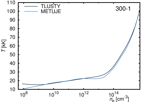
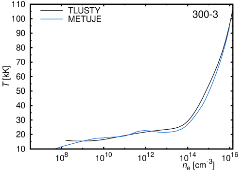
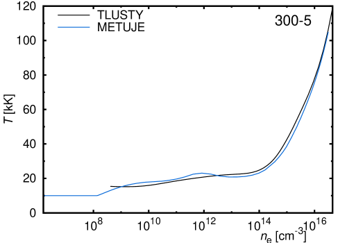
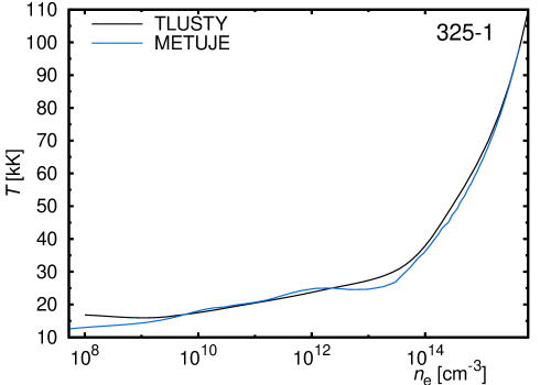
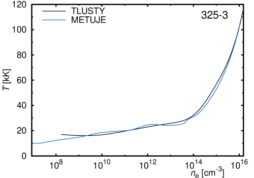
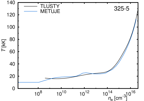
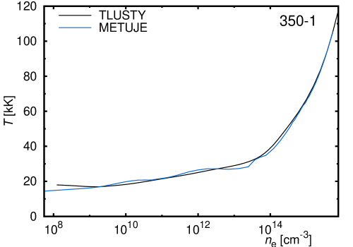
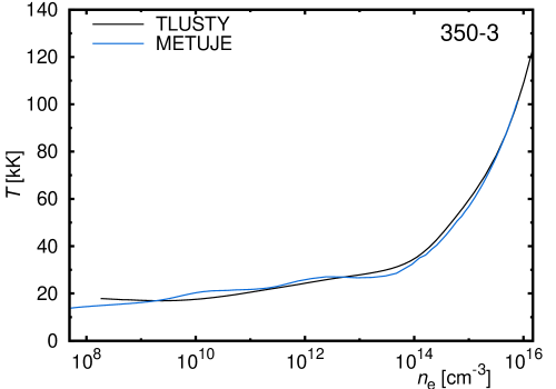
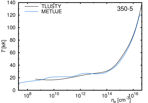
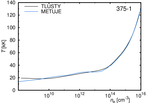
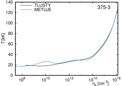
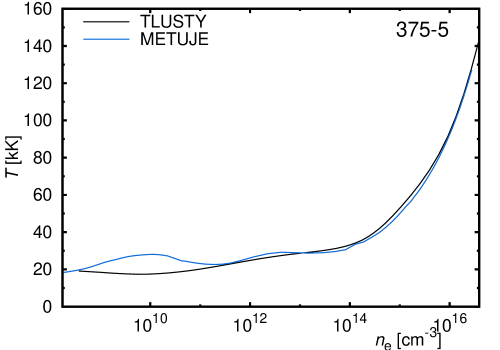
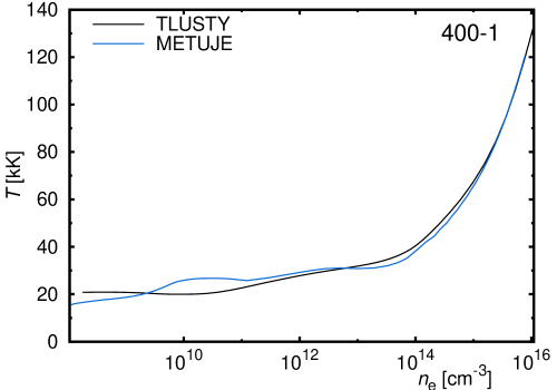
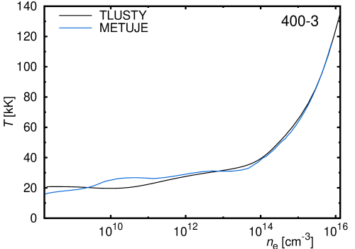
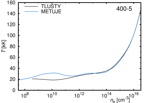
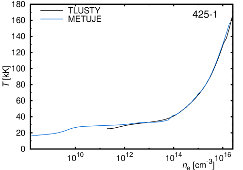
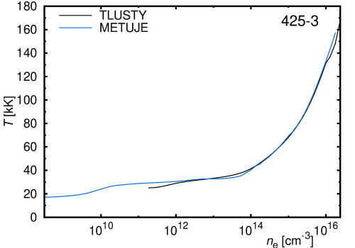
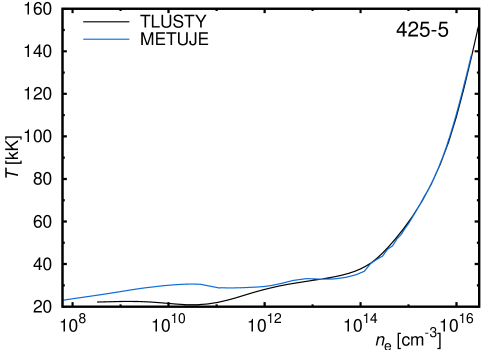
In Fig. 1 we compare the derived temperature structure of our models with results of TLUSTY (Lanz & Hubeny 2003, 2007) hydrostatic plane-parallel model atmospheres calculated for the parameters (effective temperature, surface gravity, and abundances) corresponding to our dynamic models. The temperature is plotted as a function of electron number density , which seems to be a more suitable variable for comparison of static planparallel and spherical extended dynamic models than the optical depth or column mass. The temperature structure derived from the METUJE code mostly nicely agrees with the temperature structure of TLUSTY models in deep atmospheric layers. Very small differences that are apparent especially in cooler models can be attributed to restricted iron line list in METUJE models. The atmosphere starts to expand in the low-density regions of Fig. 1 (roughly for ) resulting in larger differences between the models. In some models, a typical temperature bump caused by NLTE effects is apparent (Hubeny & Lanz 1995, Puls et al. 2005).
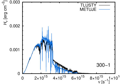
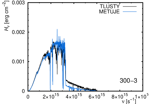
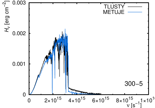
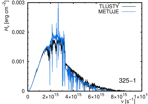
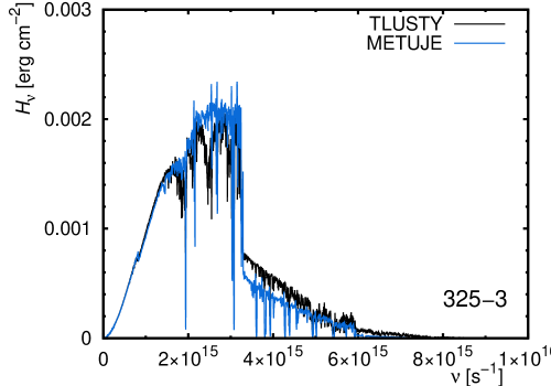
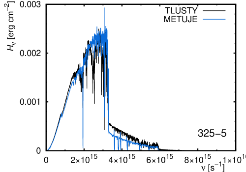
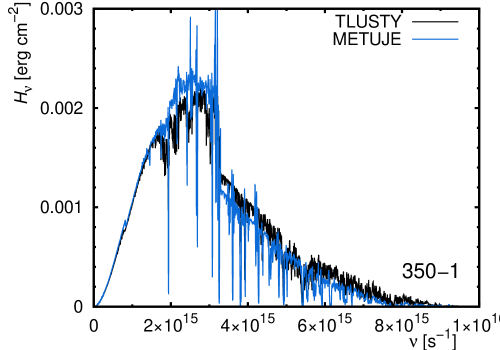
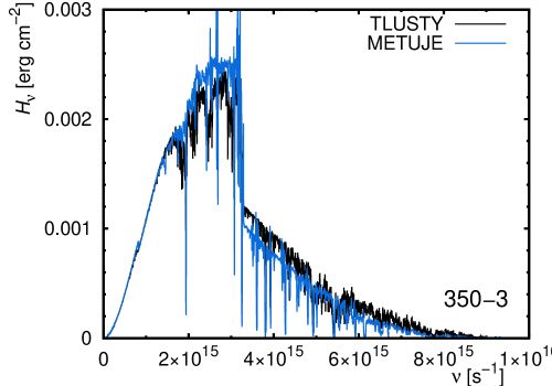
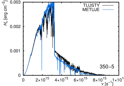
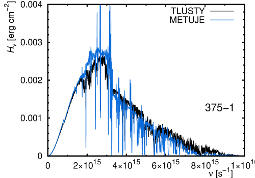
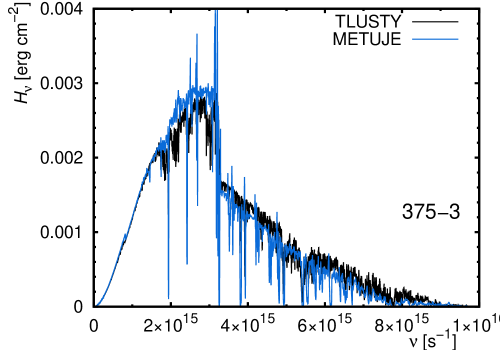
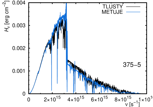
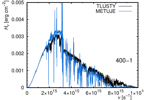
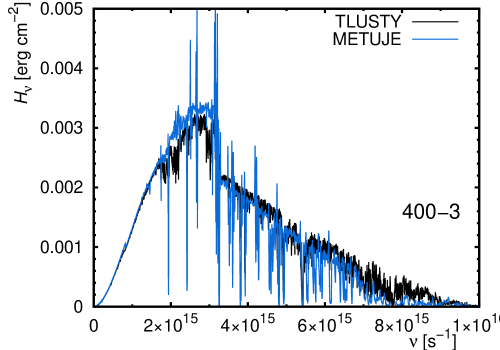
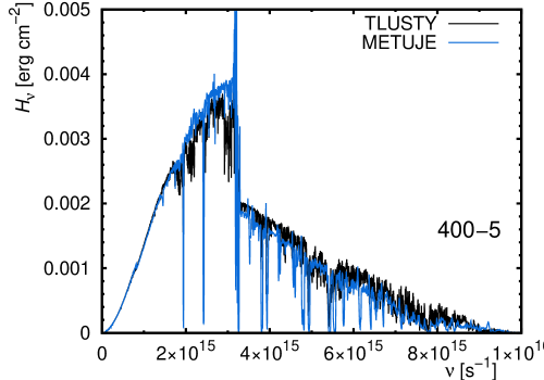
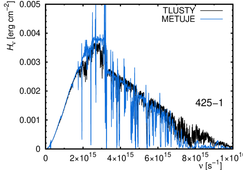
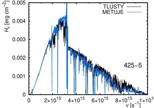
Emergent fluxes from our models also agree reasonably well with results of the TLUSTY code (see Fig. 2). The fluxes from the METUJE models were multiplied by a factor , where is the outer radius of the METUJE models, to obtain the same scale of fluxes. The fluxes nicely agree especially at lower frequencies. The flux from METUJE models is significantly lower than the flux from TLUSTY models for frequencies typically above as a result of blocking of the emergent flux by the wind. The METUJE spectrum is generally flatter; lower flux at high frequencies is accompanied with higher flux at visual frequencies. This trend has already been described for simple static spherically symmetric model atmospheres calculated without line blanketing (Kunasz et al. 1975, Kubát 1996). Small differences at higher frequencies are also connected with more elaborate line blanketing in the TLUSTY models, and with simplified treatment of the line source function in the kinetic equilibrium equations using Sobolev approximation in our models. Moreover, emission lines originating in the stellar wind appear in the emergent fluxes. The emergent fluxes from the global models also agree with results of Pauldrach et al. (2001) for frequencies lower than the He ii ionization edge. Consequently, the METUJE models provide a reasonable radiation field which is crucial for the wind modeling.
3.2 Mass-loss rates
Wind mass-loss rates scale mostly with the stellar luminosity and to a lesser extent depend on other stellar parameters (Castor, Abbott & Klein 1975, Vink et al. 2001). This dependency is also present in results of our calculations. We found that the predicted mass-loss rates very tightly correlate with the stellar luminosity. Therefore, we fitted the mass-loss rates predicted by our models (given in Table 1) as
| (11) |
which provides a relatively accurate approximation for our results with a typical error of about 10 – 20 %.
Predicted mass-loss rates from our global models agree with those derived from our older purely wind models with fixed atmospheric structure (Krtička & Kubát 2014) for stars with low luminosity and low mass-loss rates . For more luminous stars the global models give mass-loss rates roughly a factor of two lower than the purely wind models.
This difference is partly due to the effect of modified emergent flux from model atmospheres, because in previous models we used H-He model atmospheres, whereas here we include also heavier elements. Our wind models with boundary flux taken from the model atmosphere with heavier elements predict lower mass-loss rate than models with H-He atmosphere fluxes as a boundary condition. This is caused by the difference of emergent fluxes for frequencies higher above , for which H-He models predict significantly higher flux than models that include also heavier elements, where the corresponding flux is blocked (c.f., Pauldrach et al. 1994). This was tested with models in which the boundary flux was taken from model atmosphere with heavier elements for frequencies lower than and from H-He model for higher frequencies. Such combination of fluxes leads to nearly the same mass-loss rate as the models with purely H-He fluxes.
Moreover, the same frequency region is additionally blocked by the wind blanketing effect (mainly by the line transitions). The strongest blocking occurs close to the sonic point, but the high-frequency radiation is blocked in the whole wind. This blocking decreases with the distance from the stellar photosphere. The stronger blocking is connected with the fact that the wind at a given radius has higher density and, consequently, higher absorption coefficient than the hydrostatic photosphere. The blocked radiation appears at longer wavelengths as continuum and emission line radiation (Abbott & Hummer 1985, Pauldrach et al. 2001). The effect of wind blanketing is stronger for higher densities, and it is of a lesser importance for winds with low mass-loss rate. The effect of blocking was tested in the pure wind models for which we neglected acceleration from all line transitions with frequencies higher than and with boundary flux taken from the model atmosphere. These models give mass-loss rates which are close to those from global models.
Comparison with other predicted mass-loss rates
Our derived mass-loss rates are significantly lower than those predicted by Vink et al. (2001). The difference increases with luminosity and is about a factor of between two and five for stars with larger luminosity and using Anders & Grevesse (1989) solar abundances for the calculation of Vink et al. (2001) rates. The difference is about a factor of between two and four when accounting for lower solar metalicity (Asplund et al. 2009, see the rates in Table 1). Our models show similar behavior when compared to models of Pauldrach et al. (2001).
On the other hand, our predicted mass loss rate for Pup is by a factor of about 1.9 higher than the prediction of Gräfener (2003). This difference can be explained (see Krtička & Kubát 2010) as a result of strong turbulent broadening introduced in the models of Gräfener (2003). Moreover, the mass-loss rate for Pup predicted by Pauldrach et al. (1994) using realistic stellar emergent spectrum and Sobolev approximation is by a factor of higher than our predicted value for the same parameters. This could be understood as a result of the multiline effects (Puls 1987) that cause about a factor of decrease of the predicted mass-loss rate (Krtička & Kubát 2010). Our predicted mass-loss rates also reasonably agree with the predictions of Puls (1987). Sander et al. (2017) use self-consistent hydrodynamical PoWR models and for Pup they derive the mass-loss rate , which agrees reasonably well with our prediction (derived from Eq. (11) for the same luminosity) especially taking into account their adopted clumping factor .
It is not clear what exactly causes such large differences between our results and the predictions of Vink et al. (2001) and Pauldrach et al. (2001). Although the physics involved is the same, there are differences in the solution of the radiative transfer equation, in treatment of the hydrodynamics, and in derivation of the wind mass-loss rate. The most significant difference is connected to the calculation of the radiative force, especially close to the star. The models that predict large mass-loss rates in comparison to ours use the Sobolev approximation to calculate the radiative force (Vink et al. 1999, Pauldrach et al. 2012) throughout the wind. Also our models with the Sobolev approximation (Krtička & Kubát 2004) predict significantly higher mass-loss rates than the consistent CMF models presented here. Moreover, our models and the models of Gräfener (2003) use the radiative force directly in the hydrodynamical equations, whereas Vink et al. (2001) derive the mass-loss rate from global energy balance and Pauldrach et al. (2001) use line force multipliers. On the other hand, while the models of Vink et al. (2001) use the line list that includes all elements from H to Zn, we include only elements for which we solve the kinetic equilibrium equations (see Krtička & Kubát 2009).
Comparison with CMFGEN
The code CMFGEN (Hillier & Miller 1998) calculates consistent NLTE spectra of stellar atmospheres with winds assuming the velocity structure, which is usually given by a modified -velocity law (e.g., Puebla et al. 2016). The code does not solve the hydrodynamic equations. As a consequence, direct comparison with our results is not possible. However, the code can be used to calculate the radiative force and to test the consistency of derived solution. Bouret et al. (2012) for their model of Pup (see their Sect. 6.5) derive the hydrodynamically consistent solution for , for which we predict . Bouret et al. assumed the volume filling factor in their analysis (note that , the clumping factor). For a wind model with volume filling factor we predicted an increase in mass-loss rates by a factor of two (Krtička et al. 2008) with respect to a wind model without clumping. A similar situation appears for the model of Puebla et al. (2016, Fig. 18). Although their model of Ori with shows a slightly insufficient radiative force to drive the wind close to the star, our prediction gives not far from their value. Petrov et al. (2016) derive the wind mass-loss rates of BA supergiants from the requirement of energy conservation using the CMFGEN code taking into account clumping (actually microclumping). The two hottest stars from their sample with K and different masses overlap with our sample. For these stars Petrov et al. derive mass-loss rates and . This agrees with our predictions and . From this we conclude that our resulting mass-loss rates are roughly consistent with radiative force predictions derived from CMFGEN code.
Comparison with observations
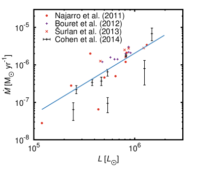
In Fig. 3 we compare the predicted dependence of the mass-loss rate on luminosity with data derived from near-infrared line spectroscopy (Najarro et al. 2011), combined optical and UV analysis that accounts for clumping (Bouret et al. 2012, Šurlan et al. 2013), and X-ray line profiles (Cohen et al. 2014). From the comparison we excluded the mass-loss rates derived from X-ray line profiles of HD 93250, which is hotter than stars considered here, and those of Ori and Oph, which have extremely low mass-loss rates for their luminosities and may display the ”weak wind problem”. When comparing with observational data, we refrained from using more common modified wind momentum (Kudritzki & Puls 2000). The wind momentum depends on the wind terminal velocity, which is sensitive to the ionization equilibrium in the outer parts of the wind. Consequently, the terminal velocity may be affected by radial variations of clumping or by X-rays (e.g., Krtička et al. 2008).
Our predictions agree with the mass-loss rates derived from X-ray line profiles (Cohen et al. 2014, Rauw et al. 2015) that were obtained with low uncertainty and with mass-loss rates derived from near-infrared emission lines (in combination with other diagnostics, Najarro et al. 2011). Our predictions are roughly a factor of 1.6 lower than those derived from combined UV and optical analysis (Bouret et al. 2012, Šurlan et al. 2013). The UV line profiles (Šurlan et al. 2013) indicate that clumping starts relatively close to the star. If the clumping has already started in the region where the mass-loss rate is determined, then it may lead to an increase of the wind mass-loss rate due to enhanced recombination (Muijres et al. 2011). Consequently, the true mass-loss rates may even be slightly higher.
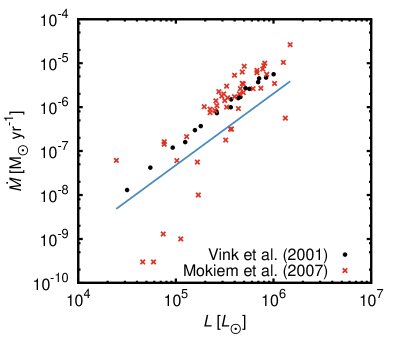
Our predicted mass-loss rates are a factor of lower than unclumped mass-loss rates derived from H line (as compiled by Mokiem et al. 2007, see Fig. 4). Taking into account clumping, the H mass-loss rates would be lower by a factor , where is the clumping factor. Attributing the difference between our predictions and compilation of Mokiem et al. (2007) to clumping would therefore imply the clumping factor of . On the other hand, in the case in which the clumping starts close to the star, the clumping also affects the theoretical predictions (Muijres et al. 2011). For optically thin inhomogeneities (microclumping) present throughout the whole wind, the mass-loss rate scales on average as with (Muijres et al. 2011, Table 3). Consequently, if the difference between the predicted and H mass-loss rates stems from the influence of clumping on both observations and predictions, then the required clumping factor is from equal . This would also imply that the true mass-loss rates are by a factor of higher than our predicted values and agree with results of Bouret et al. (2012) and Šurlan et al. (2013). However, if the clumping starts above the critical point, the difference between observation and theory would imply clumping factor , since the mass-loss rate is determined in the region below the critical point.
The difference between microclumping and macroclumping is crucial for further mass-loss rate analysis. For example, the clumping factors adopted by Bouret et al. (2012) and which account only for microclumping are somehow larger than those found by Šurlan et al. (2013), who took a more general model of macroclumping into account. The solution degeneracy in a clumped wind with interclump media may complicate the empirical mass-loss rate determination from UV lines (Šurlan et al. 2012, Sundqvist et al. 2014). Moreover, a detailed multiwavelength analysis of Ori Aa1 (Shenar et al. 2015) gives a mass-loss rate which is about a factor of three higher than the value predicted here and which agrees with predictions of Vink et al. (2001).
3.3 Terminal velocities and ionization fractions


From the theoretical considerations it follows that the wind terminal velocity is proportional to the escape speed (Castor, Abbott & Klein 1975). Lamers et al. (1995) derived an average ratio for Galactic O stars. Our models predict slightly lower ratio . The difference could possibly be caused by clumping, which we did not consider in our models. Observational analysis typically assumes that clumping increases with radius close to the star (e.g., Najarro et al. 2011, Bouret et al. 2012). Enhanced clumping in the region above the critical point causes increase of the terminal velocity (Krtička et al. 2008).
In Fig. 5 we plot the ionization fraction of selected ions at radius where as a function of the stellar effective temperature. In our calculations we do not consider any source of enhanced X-ray radiation, which may cause X-ray ionization (Cassinelli & Olson 1979, MacFarlane et al. 1994, Pauldrach et al. 2001, Krtička & Kubát 2009, Carneiro et al. 2016) and we also do not consider clumping (Hamann et al. 2008, Muijres et al. 2011). These effects may influence the comparison of our results with observations. Nonetheless, except for that of C vi, the ionization fractions agree fairly well with observations. Moreover, our calculated ionization fractions agree with those ionization fractions calculated by Carneiro et al. (2016, Fig. 8) which ignore the X-ray ionization.
4 Discussion and conclusions
We provide global (unified) wind models of O stars, which account for the stellar photosphere and wind. The models are obtained by simultaneous solution of hydrodynamic, radiative transfer, and kinetic equilibrium (NLTE) equations throughout the photosphere and wind. We provide a formula that predicts the wind mass-loss rate as a function of stellar luminosity for O stars with solar chemical composition.
As found by Bouret et al. (2012) and Puebla et al. (2016), some calculations with prespecified wind velocity law predict too low radiative acceleration around the sonic point. However, the prespecified velocity law does not necessarily fulfill the momentum equation. On the other hand, our models smoothly pass from the stellar photosphere in hydrostatic equilibrium to the fast radiativelly accelerated wind. This shows that consistent wind models that properly treat the momentum equation at the wind base are able to solve the problem of hydrodynamical consistency.
We compare our models with other models available in literature and with observations. Our models provide very similar atmospheric structure to TLUSTY models deep in the stellar atmosphere. The emergent flux from our models also reasonably agrees with TLUSTY models, and the differences between both models can be attributed mostly to the wind blanketing and to the effects caused by differences between plane-parallel and spherically symmetric model atmospheres (Kunasz et al. 1975, Kubát 1996).
With respect to our previous models that did not include the photosphere consistently, the derived mass-loss rates are on average lower by a factor of two. This is caused by stronger blocking of the radiative flux for frequencies higher than about , for which the stellar wind is still optically thick for lower velocities.
Our models provide significantly lower mass-loss rates than the models of Pauldrach et al. (2001) and Vink et al. (2001). Both these latter models use the Sobolev approximation for the calculation of the radiative force, which is not appropriate close to the star and in the case of line overlaps. Moreover, neither of these models solves the radiation hydrodynamics completely selfconsistently. Vink et al. (2001) use a prespecified hydrodynamical structure and a global energy balance to derive the mass-loss rate and Pauldrach et al. (2001) use line force multipliers to calculate the radiative force. Calculation of Müller & Vink (2008) which aims to provide hydrodynamic models with Monte Carlo radiative transfer, but with the Sobolev approximation, still provides mass-loss rate of an OV star which is about three times higher than our prediction. The Sobolev approximation provides reliable results for the calculation of radiative force coming from single line in supersonic wind (Krtička & Kubát 2010), but the simple single line Sobolev approximation that neglects continuum fails to treat multiline effects, influence of the lines on continuum, and does not provide reliable results in the vicinity of the sonic point. We conclude that the most probable reason for the lower mass-loss rate obtained by our models is an improved calculation of the line force, which is done using the CMF approach, in contrast to the Sobolev approximation, which was used in studies mentioned here.
On the other hand, our predicted mass-loss rate for Pup is slightly higher than that predicted by hydrodynamic calculations of Gräfener (2003) using the CMF line force. Moreover, our calculations are consistent with the radiative force derived from the CMFGEN code, which also uses the more general CMF method of solution of the radiative transfer equation.
The radiative force is proportional to the product of the flux and opacities. Consequently, all differences in the mass-loss rate should be attributed either to the differences in fluxes or opacities at last. Our detailed comparison with fluxes presented in Pauldrach et al. (2001) has not revealed any significant differences between the models that could cause a significant difference between predicted mass-loss rates. The difference in opacities may be caused either by inaccurate level populations or by missing opacities. However, we found reasonable agreement with ionization fractions calculated by Carneiro et al. (2016). Our tests using line data from different sources have not revealed any significant opacity gap for lighter elements with . There are some missing iron lines in the list, however their inclusion has not led to a significant increase of the radiative force. Consequently, there is likely a different reason for the difference of mass-loss rate between individual models.
Our derived mass-loss rates agree with observational results corrected for clumping. The predicted mass-loss rates agree nicely with mass-loss rates derived from X-ray line profiles (Cohen et al. 2014) and based on near-infrared lines (Najarro et al. 2011). Our derived mass-loss rates are slightly lower than mass-loss rates determined mainly from UV line profiles (Bouret et al. 2012, Šurlan et al. 2013). On the other hand, our predictions are a factor of about lower than H mass-loss rate estimates that were not corrected for clumping (as compiled by Mokiem et al. 2007). Our results can be reconciled with these H estimates assuming a clumping factor of at least .
Our predictions do not account for clumping. This is not a problem if the clumping starts above the critical point, since the mass-loss rate is determined below the critical point. However, if clumping starts relatively close to the star (Šurlan et al. 2013), then the neglect of clumping may lead to the underestimation of the predicted mass-loss rates. Consequently, the actual mass-loss rates may be slightly higher (Krtička et al. 2008, Muijres et al. 2011). The higher mass-loss rates may be also supported by the fact that the analysis of Šurlan et al. (2013) that accounts for optically thin and optically thick clumps gives systematically higher mass-loss rates than predicted by us.
Our models still used the Sobolev approximation to calculate the radiative bound-bound rates in the kinetic equilibrium equations. However, our test calculations of bound-bound rates using CMF mean intensity showed that for many of these rates the Sobolev approximation provides reliable estimate of the radiation field mean intensity in the wind. Consequently, we expect that the usage of Sobolev approximation to calculate the bound-bound rates has no significant effect on the final model. On the other hand, the saving in computing time is considerable.
From the discussion above it is not surprising that different codes predict different ionization fluxes for Å as found, for example, by Puls et al. (2005). The flux in this region is formed in the wind and is therefore sensitive to the detailed density structure of the adopted model (see also Sander et al. 2015). This is not derived consistently in many models, which may be one of the reasons for the difference of emergent fluxes derived from individual models in the far UV region.
We have shown that global wind models predict wind mass-loss rate that agree with empirical estimations (that were corrected for microclumping) within a factor of about 1.6. This result shows a promising perspective for reconciling all types of mass-loss rate determination in hot stars.
Acknowledgements.
This work was supported by grant GA ČR 13-10589S.References
- Abbott (1980) Abbott, D. C. 1980, ApJ, 242, 1183
- Abbott & Hummer (1985) Abbott, D. C., & Hummer, D. G. 1985, ApJ, 294, 286
- Anders & Grevesse (1989) Anders, E, & Grevesse, N. 1989, Geochimica et Cosmochimica Acta, 53, 197
- Asplund et al. (2009) Asplund, M., Grevesse, N., Sauval, A. J., & Scott, P. 2009, ARA&A, 47, 481
- Auer (1971) Auer, L. H. 1971, J. Quant. Spec. Radiat. Transf., 11, 573
- Auer (1976) Auer, L. H. 1976, J. Quant. Spec. Radiat. Transf., 16, 931
- Bouret et al. (2012) Bouret, J.-C., Hillier, D. J., Lanz, T., & Fullerton, A. W. 2012, A&A, 544, A67
- Bouret et al. (2013) Bouret, J.-C., Lanz, T., Martins, F., et al., 2013, A&A, 555, A1
- Cantiello et al. (2009) Cantiello, M., Langer, N., Brott, I. et al. 2009, A&A, 499, 279
- Carneiro et al. (2016) Carneiro, L. P., Puls, J., Sundqvist, J. O., & Hoffmann, T. L. 2016, A&A, 590, A88
- Cassinelli & Olson (1979) Cassinelli, J. P., & Olson, G. L. 1979, ApJ, 229, 304
- Castor, Abbott & Klein (1975) Castor, J. I., Abbott, D. C., & Klein, R. I. 1975, ApJ, 195, 157
- Chiosi & Nasi (1974) Chiosi, C., & Nasi, E. 1974, A&A, 34, 355
- Cohen et al. (2014) Cohen, D. H., Wollman, E. E., Leutenegger, M. A., et al. 2014, MNRAS, 439, 908
- Crowther et al. (2002) Crowther P. A., Hillier D. J., Evans C. J., Fullerton A. W., De Marco O., Willis A. J., 2002, ApJ 579, 774
- Crowther et al. (2006) Crowther, P. A., Lennon, D. J., & Walborn, N. R. 2006, A&A, 446, 279
- Daley-Yates et al. (2016) Daley-Yates, S., Stevens, I. R., & Crossland, T. D. 2016, MNRAS,
- De Loore et al. (1977) De Loore, C., De Greve, J. P., & Lamers, H. J. G. L. M. 1977, A&A, 61, 251
- Evans et al. (2004) Evans, C. J., Crowther, P. A., Fullerton, A. W., & Hillier, D. J. 2004, ApJ, 610, 1021
- Feldmeier et al. (1997) Feldmeier, A., Puls, J., & Pauldrach, A. W. A. 1997, A&A, 322, 878
- Feldmeier et al. (2003) Feldmeier, A., Oskinova, L., Hamann, W.-R., 2003, A&A, 403, 217
- Fullerton et al. (2006) Fullerton, A. W., Massa, D. L., Prinja, R. K., 2006, ApJ, 637, 1025
- Gabler et al. (1989) Gabler, R., Gabler, A., Kudritzki, R. P., Puls, J., & Pauldrach, A. 1989, A&A, 226, 162
- Gräfener (2003) Gräfener, G. 2003, Stellar Atmosphere Modeling, 288, 533
- Gräfener & Hamann (2005) Gräfener, G., & Hamann, W.-R. 2005, A&A, 432, 633
- Gräfener & Hamann (2008) Gräfener G., & Hamann W.-R., 2008, A&A, 482, 945
- Hamann et al. (2008) Hamann W.-R., Feldmeier A., Oskinova L. (eds.), 2008, Clumping in Hot Star Winds, Universitätsverlag Potsdam, Potsdam
- Hillier & Miller (1998) Hillier, D. J., & Miller, D. L. 1998, ApJ, 496, 407
- Hempe & Schönberg (1986) Hempe, K., & Schönberg, K. 1986, A&A, 160, 141
- Howarth & Prinja (1989) Howarth I. D., Prinja R. K., 1989, ApJS, 69, 527
- Hubeny (1988) Hubeny, I. 1988, Comput. Phys. Commun., 52, 103
- Hubeny & Lanz (1992) Hubeny, I., & Lanz, T., 1992, A&A, 262, 501
- Hubeny & Lanz (1995) Hubeny, I., & Lanz, T. 1995, ApJ 439, 875
- Hubeny & Mihalas (2014) Hubeny, I., & Mihalas, D., 2014, Theory of Stellar Atmospheres (Princeton University Press, Princeton)
- Hummer et al. (1993) Hummer, D. G., Berrington, K. A., Eissner, W., et al. 1993, A&A, 279, 298
- Ignace & Gayley (2002) Ignace R., Gayley K. G., 2002, ApJ, 568, 954
- Jiang et al. (2015) Jiang, Y.-F., Cantiello, M., Bildsten, L., Quataert, E., & Blaes, O. 2015, ApJ, 813, 74
- Keszthelyi et al. (2017) Keszthelyi, Z., Puls, J., & Wade, G. A. 2017, A&A, 598, A4
- Krtička & Kubát (2004) Krtička, J., & Kubát, J. 2004, A&A, 417, 1003
- Krtička & Kubát (2009) Krtička, J., & Kubát, J. 2009, MNRAS, 394, 2065
- Krtička & Kubát (2010) Krtička, J., & Kubát, J. 2010, A&A, 519, A5
- Krtička & Kubát (2014) Krtička, J., & Kubát, J. 2014, A&A, 567, A63
- Krtička et al. (2008) Krtička J., Muijres L., Puls J., Kubát J., de Koter A., 2008, in Deng L., Chan K. L., eds., IAU Symp. Vol. 252, The Art of Modeling Stars in the 21st Century. Cambridge Univ. Press, Cambridge, p. 283
- Kubát (1996) Kubát, J. 1996, A&A, 305, 255
- Kubát et al. (1999) Kubát, J., Puls, J., & Pauldrach, A. W. A. 1999, A&A, 341, 587
- Kudritzki & Puls (2000) Kudritzki, R. P., & Puls, J. 2000, ARA&A, 38, 613
- Kunasz et al. (1975) Kunasz, P. B., Hummer, D. G., & Mihalas, D., 1975, ApJ 202, 92
- Kupka et al. (1999) Kupka, F., Piskunov, N. E., Ryabchikova, T. A., Stempels, H. C., & Weiss, W. W. 1999, A&AS, 138, 119
- Lamers et al. (1995) Lamers, H. J. G. L. M., Snow, T. P., & Lindholm D. M. 1995, ApJ, 455, 269
- Lamers et al. (1999) Lamers, H. J. G. L. M., Haser, S., de Koter, A., & Leitherer, C., 1999, ApJ 516, 872
- Lanz & Hubeny (2003) Lanz, T., & Hubeny, I. 2003, ApJS, 146, 417
- Lanz & Hubeny (2007) Lanz, T., & Hubeny, I. 2007, ApJS, 169, 83
- Lucy & Solomon (1970) Lucy, L. B., Solomon, P. M. 1970, ApJ, 159, 879
- MacFarlane et al. (1991) MacFarlane, J. J., Cassinelli, J. P., Welsh, B. Y., et al. 1991, ApJ, 380, 564
- MacFarlane et al. (1994) MacFarlane, J. J., Cohen, D. H., & Wang, P. 1994, ApJ, 437, 351
- Martins et al. (2005a) Martins, F., Schaerer, D., & Hillier, D. J. 2005a, A&A, 436, 1049
- Martins et al. (2005b) Martins, F., Schaerer, D., Hillier, D. J., et al. 2005b, A&A, 441, 735
- Massa et al. (2003) Massa D., Fullerton A. W., Sonneborn, G., Hutchings J. B., 2003, ApJ, 586, 996
- Mihalas et al. (1975) Mihalas, D., Kunasz, P. B., & Hummer, D. G. 1975, ApJ, 202, 465
- Mokiem et al. (2005) Mokiem, M. R., de Koter, A., Puls, J., et al. 2005, A&A, 441, 711
- Mokiem et al. (2007) Mokiem, M. R., de Koter, A., Vink, J. S., et al. 2007, A&A, 473, 603
- Muijres et al. (2011) Muijres L., de Koter A., Vink J., Krtička J., Kubát J., Langer N., 2011, A&A, 526, A32
- Müller & Vink (2008) Müller, P. E., Vink, J. S. 2008, A&A, 492, 493
- Najarro et al. (2011) Najarro, F., Hanson, M. M., & Puls, J. 2011, A&A, 535, A32
- Oskinova (2016) Oskinova, L. M. 2016, Advances in Space Research, 58, 739
- Oskinova et al. (2007) Oskinova, L. M., Hamann, W.-R., & Feldmeier, A. 2007, A&A, 476, 1331
- Owocki & Puls (1999) Owocki, S. P., & Puls, J. 1999, ApJ, 510, 355
- Owocki et al. (1988) Owocki, S. P., Castor, J. I., & Rybicki, G. B. 1988, ApJ, 335, 914
- Pauldrach et al. (1994) Pauldrach A. W. A., Kudritzki R. P., Puls, J., Butler K., Hunsinger J., 1994, A&A, 283, 525
- Pauldrach et al. (2001) Pauldrach, A. W. A., Hoffmann, T. L., & Lennon, M. 2001, A&A, 375, 161
- Pauldrach et al. (2012) Pauldrach A. W. A., Vanbeveren D., Hoffmann T. L., 2012, A&A, 538, A75
- Petrov et al. (2016) Petrov, B., Vink, J. S., & Gräfener, G. 2016, MNRAS, 458, 1999
- Piskunov et al. (1995) Piskunov, N. E., Kupka, F., Ryabchikova, T. A., Weiss, W. W., & Jeffery, C. S. 1995, A&AS, 112, 525
- Puebla et al. (2016) Puebla, R. E., Hillier, D. J., Zsargó, J., Cohen, D. H., & Leutenegger, M. A. 2016, MNRAS, 456, 2907
- Puls (1987) Puls, J. 1987, A&A, 184, 227
- Puls et al. (2005) Puls, J., Urbaneja, M. A., Venero, R., et al. 2005, A&A, 435, 669
- Puls at al. (2006) Puls J., Markova N., Scuderi S., Stanghellini C., Taranova O. G., Burnley A. W., Howarth I. D., 2006, A&A, 454, 625
- Puls et al. (2008) Puls, J., Markova, N., & Scuderi, S. 2008, in Mass Loss from Stars and the Evolution of Stellar Clusters, ed. A. de Koter, L. Smith & R. Waters, (ASP, San Francisco), 101
- Rauw et al. (2015) Rauw, G., Hervé, A., Nazé, Y., et al. 2015, A&A, 580, A59
- Repolust et al. (2004) Repolust, T., Puls, J., & Herrero, A. 2004, A&A, 415, 349
- Runacres & Owocki (2002) Runacres M. C, Owocki S. P., 2002, A&A 381, 1015
- Rybicki & Hummer (1978) Rybicki, G. B., & Hummer, D. G. 1978, ApJ, 219, 654
- Rybicki & Hummer (1992) Rybicki G. B., & Hummer D. G., 1992, A&A, 262, 209
- Sander et al. (2015) Sander, A., Shenar, T., Hainich, R., et al. 2015, A&A, 577, A13
- Sander et al. (2017) Sander, A. A. C., Hamann, W.-R., Todt, H., Hainich, R., & Shenar, T. 2017, arXiv:1704.08698
- Scuderi et al. (1998) Scuderi, S., Panagia, N., Stanghellini, C., Trigilio, C., & Umana, G., 1998, A&A 332, 251
- Seaton et al. (1992) Seaton, M. J., Zeippen, C. J., Tully, J. A., et al. 1992, Rev. Mexicana Astron. Astrofis., 23, 19
- Shenar et al. (2015) Shenar, T., Oskinova, L., Hamann, W.-R., et al. 2015, ApJ, 809, 135
- Sundqvist et al. (2010) Sundqvist, J. O., Puls, J., & Feldmeier, A. 2010, A&A, 510, A11
- Sundqvist et al. (2011) Sundqvist J. O., Puls J., Feldmeier, A., Owocki S. P., 2011, A&A, 528, A6
- Sundqvist et al. (2014) Sundqvist, J. O., Puls, J., & Owocki, S. P. 2014, A&A, 568, A59
- Šurlan et al. (2012) Šurlan B., Hamann W.-R., Kubát J., Oskinova L., Feldmeier A., 2012, A&A 541, A37
- Šurlan et al. (2013) Šurlan, B., Hamann, W.-R., Aret, A., et al. 2013, A&A, 559, A130
- Thomas & Feldmeier (2016) Thomas, T., & Feldmeier, A. 2016, MNRAS, 460, 1923
- Vink et al. (1999) Vink, J. S., de Koter, A., & Lamers, H. J. G. L. M. 1999, A&A, 350, 181
- Vink et al. (2001) Vink, J. S., de Koter, A., & Lamers, H. J. G. L. M. 2001, A&A, 369, 574