Correlation Energy of Proton-Neutron Subsystem in Valence Orbit

Abstract

Deuteron correlation energy (DCE) of the valence proton-neutron subsystem is evaluated by utilizing a simple three-body model. We focus on the ⁶Li and ¹⁸F nuclei assuming the doubly-closed core and the valence proton and neutron. Two interaction models, schematic density-dependent contact (SDDC) and Minnesota potentials, are utilized to describe the proton-neutron interaction. Evaluating DCE, we conclude that the proton-neutron binding in ⁶Li can be stronger than its counterpart of a deuteron in vacuum. On the other hand, in ¹⁸F, the energetic correlation is remarkably weak, and does not favor the bound, deuteron-like configuration. This significant difference between two systems can be understood from a competition between the proton-neutron kinetic and pairing energies, which are sensitive to the spatial extension of the wave function. This result indicates a remarkable dependence of the deuteron correlation to its environment and the valence orbits.

I Introduction

Deuteron ($J^{\pi}=1^{+},S=1$) is the only possible bound system of two nucleons in vacuum. This common sentence in nuclear physics indicates that, in the spin-triplet (isospin-singlet) channel, nuclear attraction is stronger than that in the spin-singlet (isospin-triplet) channel. In spite of this unique importance, the spin-triplet proton-neutron (pn) subsystem in finite nuclei has been less investigated Csótó and Lovas (1992); Evans et al. (1981); Poves and Martinez-Pinedo (1998); Goodman (1999); Bertsch and Luo (2010); Gezerlis et al. (2011) than the spin-singlet pair of the same type of nucleons Brink and Broglia (2005); Broglia and Zelevinsky (2013); Dean and Hjorth-Jensen (2003); Bender et al. (2003).

Thanks to the recent developments of radioactive isotope-beam experiments, the access to the spin-triplet pn-pairing correlation in $N=Z$ nuclei is getting possible. In these nuclei, in which the valence proton and neutron occupy the same major shell, pn correlation is expected to be very relevant. Comparing this proton-neutron subsystem with that in vacuum, a natural question arises: “Does a proton-neutron pair at the surface of the nucleus behave like a deuteron ?”

The answer to the previous question is, however, not simple to address Shanley (1969); Csótó and Lovas (1992); Csótó (1994); Lisetskiy et al. (1999); Tursunov et al. (2007); Michel et al. (2010); Ikeda et al. (2010); Tanimura et al. (2012); Sagawa et al. (2013); Tanimura et al. (2014); Kanada-En’yo and Kobayashi (2014); Masui and Kimura (2016); Tanimura and Sagawa (2016). In recent theoretical studies, it has been shown that the spin-orbit splitting is a key feature of the deuteron correlation in nuclei. Utilizing the labels, $j_{\gtrless}\equiv l\pm 1/2$ to indicate the spin-orbit partners in the same shell, the pn correlation becomes enhanced when the energy gap between $j_{>}$ and $j_{<}$ is small Poves and Martinez-Pinedo (1998); Sagawa et al. (2013); Tanimura et al. (2014). Indeed, a strong spin-triplet pn coupling, possibly with spatial localization that indicates a sort of deuteron condensation at the surface of the nucleus, has been predicted Tanimura et al. (2014); Kanada-En’yo and Kobayashi (2014); Masui and Kimura (2016). In Ref. Masui and Kimura (2016), the importance of mixing with continuum states in the pn correlation was also shown. The quasi-deuteron configuration Lisetskiy et al. (1999), as well as the isospin-singlet condensate Bertsch and Luo (2010); Gezerlis et al. (2011), in heavy nuclei have been discussed with similar intents. It is worthwhile to remind that a similar discussion on the spin-singlet dineutron and diproton correlation has been also carried out von Oertzen and Vitturi (2001); Matsuo et al. (2005); Matsuo (2006); Bertulani and S. Hussein (2007); Margueron et al. (2007, 2008); Kikuchi et al. (2010); Hagino and Sagawa (2005); Hagino et al. (2007); Hagino and Sagawa (2007); Hagino et al. (2008); Dasso and Vitturi (2009); Oishi et al. (2010); Kanada-En’yo et al. (2011); Shimoyama and Matsuo (2013); Fortunato et al. (2014); Lay et al. (2016); Singh et al. (2016).

In spite of all the accumulated knowledge, it is still an open question whether the pn pair can be considered as bound or not in finite nuclei Wildermuth and Tang (1977). Especially, its dependence on the selected orbit(s) or on the stability of the whole system has not been clarified as yet. This information should be essential also for the phenomenology of the Gamow-Teller transition Bender et al. (2002); Roca-Maza et al. (2012), nuclear magnetic mode Lisetskiy et al. (1999); Tursunov et al. (2007); Tanimura et al. (2014) and meta-stable states Tursunov et al. (2007); Michel et al. (2010).

In this article, we present a phenomenological evaluation of the so-called deuteron-correlation energy (DCE). We also investigate its sensitivity to the properties of finite nuclei by comparing two systems: ⁶Li and ¹⁸F.

Concerning the first topic, we employ core-orbital three-body model, assuming a doubly-closed core plus the valence proton and neutron. Then, we evaluate the mean energy of the partial pn Hamiltonian, which can be well separated from the total energy. An advantage of our definition of DCE is that it becomes equivalent to the deuteron binding energy, if the pn subsystem is isolated. Thus, it gives us direct information on the changes that appear in finite systems with respect to the counterpart in vacuum.

For the second topic, we discuss the deuteron correlation in valence orbits in light $N=Z$ nuclei, ⁶Li and ¹⁸F. By evaluating DCE in three-body systems, we can investigate the sensitivity of deuteron-like subsystem to its environment. Here we point out a qualitative difference between these two systems: in ¹⁸F, the $A=17$ core-nucleon subsystem are bound, whereas this is not the case for the $A=5$ subsystems of ⁶Li. Thus, it is suitable to compare the deuteron correlation in systems where it is strongly or weakly bound. We also discuss the reliability of several interaction models, which play an essential role in the deuteron correlation problem. For simplicity, in this article, we utilize only the two-body interactions, which should be tuned for each subsystem.

In Sec.II, the formalism of our three-body model is presented. Our results and discussion for ⁶Li are also summarized there. Section III is devoted to ¹⁸F, with a comparison to ⁶Li. Finally, in Sec.IV, we summarize the main points of this article, as well as the possible improvements for future studies.

II ⁶Li Nucleus

II.1 Three-Body Model

Our investigation starts with the ⁶Li nucleus, employing the core-orbital coordinates, $\left\{\bm{r}_{p},\bm{r}_{n}\right\}$, for the three-body system, $\alpha+p+n$. The detailed formalism of these coordinates is summarized in Appendix. Within this framework, our three-body Hamiltonian is given as,

$$H_{3b} = h_{p}+h_{n}+x_{\rm rec}+v_{\rm p-n}(\bm{r}_{p},\bm{r}_{n}),$$

$$h_{i} = \frac{p_{i}^{2}}{2\mu_{i}}+V_{c-i}(r_{i}),$$

$$x_{\rm rec} = \frac{\bm{p}_{p}\cdot\bm{p}_{n}}{m_{c}}~{}~{}~{}({\rm recoil~{}term}),$$ (1)

where $i=p$ and $n$ for the valence proton and neutron, respectively. Here, $\bm{r}_{i}$ is the relative coordinate between the core and the $i$-th nucleon. Mass parameters are fixed as follows: $\mu_{i}=m_{i}m_{c}/(m_{i}+m_{c})$, $m_{p}=938.272$ MeV$/c^{2}$, $m_{n}=939.565$ MeV$/c^{2}$, and $m_{c}=3727.379$ MeV$/c^{2}$ ($\alpha$-particle mass). Namely, $h_{i}$ is the single particle (s.p.) Hamiltonian between the core and the $i$-th nucleon.

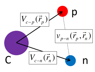
FIG. 1: Three-body model with the core and the valence proton and neutron.

The core-nucleon potential is taken as

$$V_{c-i}(\bm{r}_{i})=V_{WS}(\bm{r}_{i})+V_{Coul}(\bm{r}_{i})\delta_{i,p},$$ (2)

where the Coulomb potential of an uniformly charged sphere with radius $R_{0}$ is included for the core-proton subsystem only. For nuclear force, a Woods-Saxon plus spin-orbit potential is employed as

$$V_{WS}(r) = V_{0}f(r)+U_{ls}(\bm{l}\cdot\bm{s})\frac{1}{r}\frac{df(r)}{dr},$$ (3)

$$f(r) = \frac{1}{1+e^{(r-R_{0})/a_{0}}},$$ (4)

where $f(r)$ is a standard Fermi profile. In this paper, we adopt the parameters as $R_{0}=r_{0}\cdot 4^{1/3}$, $r_{0}=1.25$ fm, $a_{0}=0.65$ fm, $V_{0}=-47.4$ MeV, and $U_{ls}=-0.4092V_{0}r_{0}^{2}$ Esbensen et al. (1997); Hagino and Sagawa (2005). From phase-shift analysis, we confirmed that this parameter set fairly reproduces the empirical $\alpha-n$ and $\alpha-p$ scattering data in the $(p_{3/2})$-channel Ajzenberg-Selove (1988); Tilley et al. (2002); NND , as summarized in Table 1.

We expand the relevant pn-states on an uncorrelated basis, that is the tensor product of proton and neutron states:

$$\ket{\Phi^{pn(J,\pi)}_{\kappa\lambda}}=\left[\ket{\phi^{p}_{\kappa}}\otimes\ket{\phi^{n}_{\lambda}}\right]^{(J,\pi)},$$ (5)

where $\kappa$ is the shorthand label for all the quantum numbers of the proton states, $\left\{n_{p},l_{p},j_{p},m_{p}\right\}$, and similarly with $\lambda$ for neutron states. Those include the radial quantum number $n$, the orbital angular momentum $l$, the spin-coupled angular momentum $j$ and the magnetic quantum number $m$. Each s.p. state satisfies,

$$h_{p}\phi^{p}_{\kappa}(\bm{r}_{p})=\epsilon_{\kappa}\phi^{p}_{\kappa}(\bm{r}_{p}),$$

$$h_{n}\phi^{n}_{\lambda}(\bm{r}_{n})=\epsilon_{\lambda}\phi^{n}_{\lambda}(\bm{r}_{n}),$$ (6)

where $\epsilon_{\kappa(\lambda)}$ is the single-proton (neutron) eigen-energy. Notice that these states describe the $A=5$ unbound systems, ⁵Li and ⁵He. We employ the s.p. states up to the $(h_{11/2,~{}9/2})$-channel ($l_{\rm max}=5$). We confirmed that this truncation provides a sufficient convergence of the ground state energy of ⁶Li. In order to take into account the Pauli principle, we exclude the first $(s_{1/2})$ state occupied by the core nucleus. The continuum s.p. states are discretized in the radial box of $R_{\rm box}=20$ fm. We also fix the energy cut-off, $E_{\rm cut}=15$ MeV, in this article. Because we limit our investigation to the low-energy region only, this truncation of model space indeed provides a sufficient convergence for our results.

TABLE 1: Resonance energy and width obtained with the alpha-nucleon potential. Those are evaluated from the scattering phase-shift in the $(p_{3/2})$-channel.

	$V_{0}$	$E_{\alpha-n},~{}\Gamma_{\alpha-n}$	$E_{\alpha-p},~{}\Gamma_{\alpha-p}$
	(MeV)	(MeV)	(MeV)
This work	$-47.4$	$0.77,~{}0.67$	$1.61,~{}1.31$
	$-49.0$	$0.54,~{}0.38$	$1.37,~{}0.94$
Exp.Ajzenberg-Selove (1988)		$0.89,~{}0.60$	$1.97,~{}(\simeq 1.5)$
Exp.Tilley et al. (2002)		$0.798,~{}0.578$	$1.69,~{}1.06$
Exp.NND		$0.735,~{}0.60$	$1.96(5),~{}(\simeq 1.5)$

II.2 Proton-Neutron Interactions

II.2.1 Schematic Density-Dependent Contact Interaction

For pn subsystem, we employ two simple interaction models in this article. Our first choice is the so-called schematic density-dependent contact (SDDC) potential Tanimura et al. (2012, 2014). That is,

$$v_{\rm p-n}(\bm{r}_{p},\bm{r}_{n}) = w\left(\left|\frac{\bm{r}_{p}+\bm{r}_{n}}{2}\right|\right)\cdot\delta(\bm{r}_{p}-\bm{r}_{n}),$$

$$w(r) = w_{0}\left[1-\eta f(r)\right],$$ (7)

where $\eta$ is an adjustment parameter. We utilize the same density profile, $f(r)$, in Eqs.(3) and (7), in order to take the schematic density-dependence into account. Notice that $w(r\rightarrow 0)=w_{0}$ for an isolated proton-neutron pair from the core. Thus, its bare strength, $w_{0}$, should be determined consistently to the energy cutoff, $E_{\rm cut}$, and the vacuum scattering length, $a_{v}^{(S)}$ Bertsch and Esbensen (1991); Esbensen et al. (1997):

$$a_{v}^{(S)}=\left[\frac{2k_{\rm cut}}{\pi}+4\pi\frac{\hbar^{2}}{2\mu_{\rm p-n}w^{(S)}_{0}}\right]^{-1}~{}~{}({\rm fm}),$$ (8)

or equivalently,

$$w_{0}^{(S)}=\frac{\hbar^{2}}{2\mu_{\rm p-n}}\cdot\frac{4\pi^{2}a_{v}^{(S)}}{\pi-2a_{v}^{(S)}k_{\rm cut}}~{}~{}({\rm MeV\cdot fm^{3}}),$$ (9)

where $\mu_{\rm p-n}=m_{p}m_{n}/(m_{p}+m_{n})$ and $k_{\rm cut}=\sqrt{2\mu_{\rm p-n}E_{\rm cut}}/\hbar$. The superscripts $S=0$ and $1$ indicate the spin-singlet and triplet channels, respectively.

In Fig.2, the relationship between the bare strength and the vacuum scattering length is presented. Empirical values are $a_{v}^{(S=0)}=-23.748$ fm and $a_{v}^{(S=1)}=5.424$ fm for the spin-singlet and triplet channels, respectively Dumbrajs et al. (1983); Babenko (2007). Since neutron and proton can become bound in the spin-triplet channel, $a_{v}^{(1)}$ is positive finite, and its corresponding bare strength, $w_{0}\simeq-2600$ MeV$\cdot{\rm fm}^{3}$ for $E_{\rm cut}=15$ MeV, provides a strong attraction in vacuum. On the other hand, in the spin-singlet channel, $a_{v}^{(0)}$ stays negative and the pairing attraction is incapable to bind the pn system.

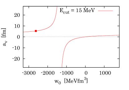
FIG. 2: Relationship between the bare contact strength and the vacuum scattering length. The empirical value of the spin-triplet pn-scattering length, $a_{v}^{(S=1)}=5.424$ fm, is indicated with a symbol.

In this article, we only deal with the $J^{\pi}=1^{+}$ configuration. Thus, from angular momentum algebra, the spin-singlet component of the pn-interaction can be neglected Tanimura et al. (2012).

II.2.2 Minnesota Interaction

As our second option, we employ the spin-triplet Minnesota potential for the pn subsystem Thompson et al. (1977); Suzuki et al. (2004); Hagino and Sagawa (2007); Myo et al. (2010, 2014). Using the spin-triplet projection, $\hat{P}_{S=1}$, that is,

$$v_{\rm p-n}(\bm{r}_{p},\bm{r}_{n}) = V^{(S=1)}_{\rm Min}(\left|\bm{r}_{p}-\bm{r}_{n}\right|)\hat{P}_{S=1},$$

$$V^{(S=1)}_{\rm Min}(r) = V_{r}e^{-K_{r}r^{2}}+V_{t}e^{-K_{t}r^{2}},$$ (10)

where $V_{r}=200$ MeV, $V_{t}=-178$ MeV, $K_{r}=1.487$ fm^-2 and $K_{t}=0.639$ fm^-2 Thompson et al. (1977). This potential correctly reproduces the deuteron binding energy, $\simeq 2.2$ MeV, for the isolated pn system.

II.3 Ground State of ⁶Li

We solve the ground state (g.s.) of ⁶Li by diagonalizing the three-body Hamiltonian. This leads to the solution,

$$\Psi^{(1,+)}_{g.s.}(\bm{r}_{p},\bm{r}_{n})=\sum_{M}U_{M}\Phi^{pn(1,+)}_{M}(\bm{r}_{p},\bm{r}_{n}),$$ (11)

with expansion coefficients, $\{U_{M}\}$. Here $M=\{\kappa,\lambda\}$ is the simplified label for the uncorrelated basis. In our computation, $M_{\rm max}\simeq 200$ basis states are employed.

TABLE 2: Ground state of ⁶Li ($1^{+}$) obtained with several pn-interaction models. The empirical three-body binding energy is $E_{3b}=-S_{\rm pn}(^{6}{\rm Li})=-3.70$ MeV NND . The 4 major configurations are also tabulated: $\pi$ and $\nu$ indicate the $\alpha$-proton and $\alpha$-neutron orbits, respectively. $E_{v}({\rm d})$ is the two-body binding energy of deuteron in vacuum, obtained with the Minnesota potential. For other quantities, see text for details.

Label	Li-S	Li-S2	Li-MO	Li-MF	Li-MO2
Type of $v_{\rm p-n}$	SDDC with $f(r)$ of $\alpha$		Minnesota for $S=1$
Adjustment of $v_{\rm p-n}$	$\eta=1.27$	$\eta=1.44$	$f=1$	$f=1.13$	$f=1$
$E_{v}({\rm d})$ (MeV)	($a_{v}^{(S=1)}=5.424$ fm)		$-2.22$	$-4.07$	$-2.22$
$V_{0}$ of WS Pot. (MeV)	$-47.4$	$-49.0$	$-47.4$	$-47.4$	$-49.0$
$E_{3b}=\Braket{H_{3b}}$ (MeV)	$-3.70$	$-3.70$	$-2.69$	$-3.70$	$-3.64$
$\Braket{v_{\rm p-n}}$ (MeV)	$-8.96$	$-8.22$	$-7.65$	$-8.91$	$-8.17$
$\Braket{x_{\rm rec}}$ (MeV)	$-0.44$	$-0.44$	$-0.38$	$-0.37$	$-0.34$
$\Braket{\theta_{\rm pn}}$ (deg)	$83.9$	$83.8$	$84.6$	$85.2$	$85.9$
$\pi(p_{3/2})\cdot\nu(p_{3/2})$ (%)	$54.7$	$56.4$	$60.4$	$58.7$	$62.5$
$\pi(p_{1/2})\cdot\nu(p_{3/2})$ (%)	$18.8$	$18.1$	$16.9$	$17.8$	$16.5$
$\pi(p_{3/2})\cdot\nu(p_{1/2})$ (%)	$18.3$	$17.7$	$16.3$	$17.3$	$15.9$
$\pi(s_{1/2})\cdot\nu(s_{1/2})$ (%)	$~{}2.9$	$~{}1.3$	$~{}2.3$	$~{}2.2$	$~{}1.3$
DCE $\equiv\Braket{h_{p-n}}$ (MeV)	$-4.34$	$-3.54$	$-3.21$	$-4.35$	$-3.46$
$\Braket{h_{c-pn}}$ (MeV)	$+0.64$	$-0.16$	$+0.52$	$+0.65$	$-0.18$
$\Braket{\pi^{2}_{p-n}/2\mu_{p-n}}$ (MeV)	$4.62$	$4.68$	$4.44$	$4.56$	$4.71$
$\Braket{\pi^{2}_{c-pn}/2\mu_{c-pn}}$ (MeV)	$4.29$	$4.84$	$4.43$	$4.63$	$5.07$
$\sqrt{\Braket{\xi^{2}_{p-n}}}$ (fm)	$5.72$	$5.55$	$5.61$	$5.64$	$5.46$
$\sqrt{\Braket{\xi^{2}_{c-pn}}}$ (fm)	$3.46$	$3.42$	$3.38$	$3.28$	$3.11$

From experimental data Ajzenberg-Selove (1988); NND , the three-body separation energy is,

$$S_{\rm pn}(^{6}{\rm Li})=S_{\rm d}(^{6}{\rm Li})+S_{\rm n}({\rm d}),$$

or equivalently,

$$\phantom{S_{\rm pn}(^{6}{\rm Li})}=S_{\rm n}(^{6}{\rm Li})+S_{\rm p}(^{5}{\rm Li})\simeq 3.70~{}~{}({\rm MeV}).$$

In order to reproduce this empirical energy, we employ $\eta=1.27$ for the SDDC potential in Eq. (7).

With the Minnesota potential, on the other hand, its original parameters fail to reproduce the empirical energy, with a positive deviation of almost $1$ MeV. Namely, for the fitting, we need an enhancement of the pn attraction. Thus, in addition, we repeat the same calculation but with the enhancement factor, $f=1.13$. That is,

$$v_{\rm p-n}(\bm{r}_{p},\bm{r}_{n})=f\cdot V^{(S=1)}_{\rm Min}(\left|\bm{r}_{p}-\bm{r}_{n}\right|)\hat{P}_{S=1}.$$ (12)

This modification, of course, leads to an inconsistency with the deuteron energy in vacuum.

In Table 2, our results with the SDDC and Minnesota interactions (original and fitted) are summarized as “Li-S”, “Li-MO”, and “Li-MF” sets. Generally, they well coincide with each other. One can find that both pn interactions play a major role: the mean pn interaction energy, $\Braket{v_{p-n}}$, shows deeply negative values within the g.s. solutions.

The mean opening angle of pn, $\Braket{\theta_{pn}}$, is less than $90$ degrees in the three cases. This indicates a spatial correlation between two nucleons Masui and Kimura (2016). Indeed, as shown in Ref. Hagino and Sagawa (2005), this is a product of the mixture of different parities with respect of the core-nucleon subsystems: if one employs only the odd or even-$l$ states in the uncorrelated basis, the resultant mean opening angle should be exactly $90$ degrees, lacking the spatial correlation. In our present result, however, this angular correlation is weak compared with the isospin-triplet dineutron or diproton correlation Hagino and Sagawa (2005); Oishi et al. (2010); Bertulani and S. Hussein (2007); Oishi et al. (2014). This is consistent with the fact that the contamination from channels other than $(p_{3/2})$ and $(p_{1/2})$ is minor in this system.

Comparing the original and enhanced Minnesota cases, indicated by Li-MO and Li-MF in Table 2, the pn interaction potential is more attractive in the latter case. This is simply due to our fitting manipulation to the empirical binding energy. However, the above structural information is qualitatively similar, and we conclude its weak sensitivity to the binding energy.

II.4 Deuteron Correlation Energy

In order to evaluate the deuteron correlation energy (DCE), it is more convenient to work with the T-Jacobi coordinates. Namely, we can transform our core-orbital coordinates, $\left\{\bm{r}_{p},\bm{r}_{n}\right\}$, to the T-Jacobi ones, $\left\{\bm{\xi}_{p-n},\bm{\xi}_{c-pn}\right\}$, as seen in Fig. 3. Exact formulas can be found in Appendix. In these T-Jacobi coordinates, our three-body Hamiltonian is decomposed as,

$$H_{3b}=h_{p-n}+h_{c-pn},$$ (13)

with two terms,

$$h_{p-n} = \frac{\pi_{p-n}^{2}}{2\mu_{p-n}}+v_{\rm p-n}(|\bm{\xi}_{p-n}|),$$

$$h_{c-pn} = \frac{\pi_{c-pn}^{2}}{2\mu_{c-pn}}+V_{c-p}(\bm{\xi}_{p-n},\bm{\xi}_{c-pn})$$ (14)

$$+V_{c-n}(\bm{\xi}_{p-n},\bm{\xi}_{c-pn}),$$

where $\bm{\pi}_{\rm p-n}$ is the relative momentum between the valence proton and neutron. Thus, $h_{p-n}$ is exactly the pn-subsystem Hamiltonian, including the SDDC or Minnesota interaction.

By taking the expectation value, $\Braket{h_{p-n}}$, we can evaluate the deuteron correlation inside the three-body system. For the pn system in vacuum, this expectation value of the ground state is, of course, the binding energy of deuteron. In the following, we employ $\Braket{h_{p-n}}$ as the definition of DCE. Note that, in some literature Sagawa et al. (2013); Masui and Kimura (2016), one can find several other definitions of DCE.

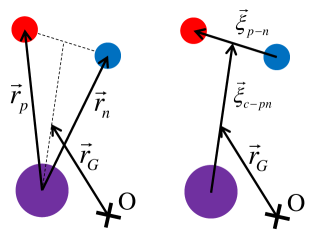
FIG. 3: Core-orbital coordinates (left) and T-Jacobi coordinates (right).

The result is displayed in the lower half of Table 2. There, we also tabulate the mean kinetic energies, $\Braket{\pi^{2}_{p-n}/2\mu_{p-n}}$ and $\Braket{\pi^{2}_{c-pn}/2\mu_{c-pn}}$. Notice that $\Braket{h_{p-n}}=\Braket{v_{\rm p-n}}+\Braket{\pi^{2}_{p-n}/2\mu_{p-n}}$ from our definition. Thus, DCE is the outcome of the competition between pairing and kinetic energies, which are negative and positive, respectively. The dependence of these terms on the selected environment is indeed the core of our problem.

From the DCE values, it can be concluded that the deuteron subsystem in ⁶Li gets an extra binding with respect to its vacuum counterpart, $-2.22$ MeV. This is a common feature in both Li-S, Li-MO, and Li-MF cases.

In the original Minnesota case (Li-MO), we emphasize that its parameters are correctly fitted so as to reproduce the binding energy, $-2.22$ MeV, if in vacuum. Even when using the same parameters, however, an enhancement of DCE around the core nucleus is not negligible. Thus, our result provides a typical case study, showing how the partial two-body system is affected by the presence of the third cluster.

Beside these interesting results, however, we should face one shortcoming, namely the instability problem in the core-pn channel: the expectation value, $\Braket{h_{c-pn}}$, is positive both in the SDDC and Minnesota cases. Thus, the core-pn subsystem should be unbound with our parameters. To remedy this problem, we employ a slightly deeper Woods-Saxon potential for the core-nucleon channels: $V_{0}=-49.0$ MeV in Eq.(3), whereas the other parameters are not changed. With this potential, the core-nucleon levels are slightly deviated from the experimental data, but the whole picture still keeps a qualitative consistency: both core-proton and core-neutron states are broad resonances, as seen in Table 1 ($V_{0}=-49.0$ MeV).

In “Li-S2” and “Li-MO2” sets in Table 2, our results with the deeper core-nucleon potential are summarized. In order to reproduce the three-body binding energy there, the SDDC interaction needs to be refitted ($\eta=1.44$), whereas the Minnesota can be unchanged from its original value. Eventually, the core-pn channel is stable with negative mean energies. Furthermore, also in these cases, our previous statement can be kept: the pn subsystem is more strongly bound (about $50$ %) than in vacuum. Consequently, in all the calculations we have performed, an enhancement of DCE has been observed.

II.5 Geometric Structure

In order to evaluate the spatial extent of the wave function, we compute the mean relative distances, $\Braket{\xi^{2}_{p-n}}$ and $\Braket{\xi^{2}_{c-pn}}$. From Appendix, the corresponding operators are given by

$$\xi^{2}_{p-n}=\left|\bm{\xi}_{p-n}\right|^{2}=\left|\bm{r}_{p}-\bm{r}_{n}\right|^{2},$$

$$\xi^{2}_{c-pn}=\left|\bm{\xi}_{c-pn}\right|^{2}=\left|(\bm{r}_{p}+\bm{r}_{n})/2\right|^{2}.$$ (15)

Thus, the mean distances depend on $\Braket{r^{2}_{p,n}}$ and $\Braket{\bm{r}_{p}\cdot\bm{r}_{n}}$. Especially for $\Braket{\xi^{2}_{p-n}}$, if the total three-body system is loosely bound with an extended wave function, this value is also large, but with a notable exception: when the resultant pn-opening angle is sufficiently narrow, then $\Braket{\xi^{2}_{p-n}}\simeq 0$.

At the bottom of Table 2, our results are tabulated. Comparing those with the kinetic energies, one can find a common feature: when the relative distance gets narrow, its corresponding kinetic energy increases. This can be naturally understood from the uncertainty principle between the relative coordinates and the conjugate momenta.

For the comparison with another system, ¹⁸F, in the next section, we point out a general feature of DCE. When the total three-body system is loosely bound, the pn-relative distance, $\Braket{\xi^{2}_{p-n}}$, is large if $\cos\Braket{\theta_{\rm pn}}\simeq 0$, and consistently, the kinetic energy, $\Braket{\pi^{2}_{p-n}/2\mu_{p-n}}$, becomes small. Consequently, the pn subsystem can get energetically “stable”, in spite of the loose stability of the whole system. In ⁶Li, indeed, this kinetic energy is not sufficient to overcome the pairing energy, and thus, the pn subsystem is quite deeply bound.

Finally, concerning the more realistic computations, of course, we admit that further optimization may be considered. Those include the exact treatment of the continuum levels in the core-nucleon channels Michel et al. (2010); Aoyama et al. (2006); Myo et al. (2014); Kruppa et al. (2014); Id Betan et al. (2002); Betan and Nazarewicz (2012); Id Betan (2017), as well as the tensor and spin-orbit components in the pn interaction Csótó and Lovas (1992); Myo et al. (2008). Those are, however, technically demanding and beyond the scope of our present model.

III ¹⁸F Nucleus

Next we focus on another system, ¹⁸F, which may also support the deuteron correlation around the core nucleus, ¹⁶O. A major difference from ⁶Li is that, in the ¹⁶O$-p$ or ¹⁶O$-n$ subsystem, there are some bound s.p. orbits. Also, the major shell includes $(s_{1/2})$, $(d_{5/2})$ and $(d_{3/2})$. Thus, it can be suitable to investigate the sensitivity of the deuteron correlation to the valence orbit(s).

TABLE 3: Core-nucleon energy levels of ¹⁷O and ¹⁷F with respect to the one-nucleon threshold, obtained with the core-nucleon potentials in this work. The unit is MeV. Subscript $r$ indicates the s.p. resonances, and $\Gamma$ is the resonance width obtained from the scattering phase-shift.

		This work		Exp.NND
		default	$pf$-mix.
16O-n	$\epsilon(2s_{1/2})$	$-3.25$		$-3.272$
	$\epsilon(1d_{5/2})$	$-4.11$		$-4.143$
	$\epsilon_{r}(d_{3/2})$	$+0.90$		$+0.941$
		($\Gamma=0.10$)		($\Gamma=0.096$)
	$\epsilon_{r}(f_{7/2})$	$+7.01$	$+4.13$	$-$
		($\Gamma=2.74$)	($\Gamma=0.58$)
	$\epsilon_{r}(f_{5/2})$	$+11.6$	$+9.48$	$-$
		($\Gamma=12.1$)	($\Gamma=6.04$)
	$\epsilon_{r}(p_{3/2})$	$+2.72$	$+0.61$	$-$
		($\Gamma=8.60$)	($\Gamma=1.15$)
16O-p	$\epsilon(2s_{1/2})$	$-0.13$		$-0.105$
	$\epsilon(1d_{5/2})$	$-0.55$		$-0.600$
	$\epsilon_{r}(d_{3/2})$	$+4.01$		$+4.40$
		($\Gamma=0.89$)		($\Gamma=1.53$)
	$\epsilon_{r}(f_{7/2})$	$+10.0$	$+7.22$	$-$
		($\Gamma=4.02$)	($\Gamma=1.29$)
	$\epsilon_{r}(f_{5/2})$	$+14.8$	$+12.6$	$-$
		($\Gamma=14.4$)	($\Gamma=7.83$)
	$\epsilon_{r}(p_{3/2})$	no reso-	$+2.94$	$-$
		nance	($\Gamma=3.58$)

TABLE 4: Same to Table 2 but for the g.s. of ¹⁸F ($1^{+}$). The empirical binding energy is $E_{3b}=-9.75$ MeV NND .

Label	F-S	F-S2	F-MO	F-MF	F-MF2
Type of $v_{\rm p-n}$	SDDC with $f(r)$ of 16O		Minnesota for $S=1$
Adjustment of $v_{\rm p-n}$	$\eta=1.32$	$\eta=1.437$	$f=1$	$f=0.67$	$f=0.59$
$E_{v}({\rm d})$ (MeV)	($a_{v}^{(S=1)}=5.424$ fm)		$-2.22$	$>0$ (unbound)
WS Pot.	default	$pf$-mix.	default	default	$pf$-mix.
$E_{3b}=\Braket{H_{3b}}$ (MeV)	$-9.78$	$-9.74$	$-13.33$	$-9.75$	$-9.72$
$\Braket{v_{\rm p-n}}$ (MeV)	$-7.17$	$-8.11$	$-11.32$	$-6.89$	$-6.90$
$\Braket{x_{\rm rec}}$ (MeV)	$-0.10$	$-0.63$	$-0.09$	$-0.07$	$-0.45$
$\Braket{\theta_{\rm pn}}$ (deg)	$87.4$	$72.3$	$88.7$	$88.7$	$80.0$
$\pi(d_{5/2})\cdot\nu(d_{5/2})$ (%)	$57.9$	$52.2$	$48.4$	$60.7$	$61.2$
$\pi(d_{3/2})\cdot\nu(d_{5/2})$ (%)	$13.9$	$10.9$	$15.0$	$10.4$	$\phantom{0}9.1$
$\pi(d_{5/2})\cdot\nu(d_{3/2})$ (%)	$13.5$	$10.2$	$15.7$	$10.5$	$\phantom{0}8.5$
$\pi(s_{1/2})\cdot\nu(s_{1/2})$ (%)	$10.7$	$10.8$	$17.6$	$16.0$	$14.6$
$\pi(f_{7/2})\cdot\nu(f_{7/2})$ (%)	$~{}0.4$	$~{}6.9$	$~{}0.2$	$0.1$	$\phantom{0}2.8$
$\pi(p_{3/2})\cdot\nu(p_{3/2})$ (%)	$~{}0.5$	$~{}1.9$	$~{}0.3$	$0.2$	$\phantom{0}0.7$
DCE $\equiv\Braket{h_{p-n}}$ (MeV)	$+0.33$	$+3.17$	$-2.05$	$+1.78$	$+4.66$
$\Braket{h_{c-pn}}$ (MeV)	$-10.11$	$-12.91$	$-11.28$	$-11.53$	$-14.38$
$\Braket{\pi^{2}_{p-n}/2\mu_{p-n}}$ (MeV)	$7.50$	$11.28$	$9.27$	$8.67$	$11.56$
$\Braket{\pi^{2}_{c-pn}/2\mu_{c-pn}}$ (MeV)	$6.59$	$\phantom{0}1.34$	$8.89$	$8.49$	$\phantom{0}4.82$
$\sqrt{\Braket{\xi^{2}_{p-n}}}$ (fm)	$5.09$	$4.73$	$4.96$	$4.95$	$4.60$
$\sqrt{\Braket{\xi^{2}_{c-pn}}}$ (fm)	$2.79$	$3.37$	$2.58$	$2.59$	$2.83$

III.1 Model Parameters

For ¹⁸F, we perform similar calculations but with an appropriate change of parameters. First, the core-mass parameter, $m_{c}$, is changed as appropriate. In order to take Pauli principle into account, we exclude the $(1s_{1/2}),(1p_{3/2}),$ and $(1p_{1/2})$ states, which are occupied by the core nucleus.

For the core-nucleon interaction, we again adopt the Woods-Saxon potential, where Coulomb term is added only for the s.p. proton states. In Eq.(2), some parameters are changed: in our default set, $R_{0}=r_{0}\cdot 16^{1/3}$, $V_{0}^{(l=0)}=-53.1$ MeV, $V_{0}^{(l\neq 0)}=0.99\cdot V_{0}^{(l=0)}$, and $U_{ls}=24.9$ MeV$\cdot$fm², while $r_{0}$ and $a_{0}$ are unchanged. In correspondence, the density profile, $f(r)$, in the SDDC pn interaction is also changed.

Additionally to the default set, in Sec. III.3, we also employ $pf$-mixture Woods-Saxon potential. There, its depth parameter is modified only for the odd-$l$ channels: $V_{0}^{(l=odd)}=1.188\cdot V_{0}^{(l=0)}$.

In Table 3, the core-nucleon levels are summarized. Our parameters fairly reproduce the experimental s.p. levels both in the proton and neutron channels. For resonant channels, we also checked the width as obtained from the phase-shift analysis. These results approximately coincide with other theoretical models Tanimura et al. (2012); Masui and Kimura (2016).

Because of the well-determined s.p. levels, in contrast to the case of ⁶Li, we cannot modify the core-nucleon potentials for the major $sd$-shell. Thus, in order to reproduce the three-body binding energy, the only adoptable way is to modify the pn interaction parameters. For ¹⁸F, this binding energy is measured as $9.75$ MeV NND . Thus, the SDDC pn-pairing interaction is re-adjusted with $\eta=1.32$. For the Minnesota interaction, on the other hand, we need a reduction factor, $f=0.67$, to reproduce this empirical energy similarly to Ref.Masui and Kimura (2016).

III.2 Ground State of ¹⁸F

In “F-S”, “F-MO”, and “F-MF” sets in Table 4, our results are summarized in the same manner as for ⁶Li. Generally, pn pairing makes a major contribution also in ¹⁸F. The mean pn interaction energy, $\Braket{v_{\rm p-n}}$, exhausts $85$ % of the three-body binding energy in the F-MO case, whereas it amounts to $70$ % in the other two cases.

Checking other results in the three cases, the structural properties are similar, and not too sensitive to the specific pn interaction models. There is a small amount of pn-angular correlation, but not very significant. This corresponds to a small mixing of the $sd$-shell with other orbits. Because of the heavy core, the recoil-term energy is almost negligible in this system. The mean relative distances also show similar values, independently of the pn interactions. These values are well consistent with the results in Ref. Tanimura et al. (2012).

III.3 Energy and Spatial Correlations

When evaluating the DCE, however, the situation becomes contrary to the initial guess of the strong deuteron correlation. First, in the original Minnesota case (F-MO), DCE is smaller than the value in vacuum. Namely, the bound $sd$-shell hardly supports the pn-energy correlation. Furthermore, comparing this DCE with other two cases (F-S and F-MF), where the pairing parameters have to be adjusted, a drastic change occurs. In the F-S and F-MF cases, the pn-subsystem is unstable around the core, because DCE is positive. This coincides with the reduction of the pairing attraction strength to achieve the empirical binding energy. Indeed, the reduced Minnesota force does not support the spin-triplet pn-bound state in vacuum: $E_{v}({\rm d})>0$. Note also that, even with the positive DCE value, the whole system can still be stable, as long as $\Braket{h_{c-pn}}$ is sufficiently negative.

Until this point, within our simple two-body interaction models, there has been no indication of an enhancement of DCE in ¹⁸F, showing a remarkable difference from ⁶Li. Also, the opening-angle or equivalently the spatial correlation is not significant. The latter result is in contrast to Ref.Masui and Kimura (2016). In order to reproduce the spatial pn correlation, and to investigate its effect on DCE, we replace the Woods-Saxon potential with the $pf$-mixture version. With this potential, as shown in Table 3, the odd-$l$ states become closer to the Fermi surface, and thus, a certain degree of mixing with the g.s. solutions is more easily realized.

In sets “F-S2” and “F-MF2” of Table 4, our results with the $pf$-mixture potential are given. Indeed, we can find an increase of the odd-$l$ contamination. Consistently, the opening angle can get closer with this potential, as we expected. Note also that, for the three-body binding energy, pn-pairing interactions are re-adjusted. In these cases with a significant spatial correlation, however, the pn subsystem is not bound in ¹⁸F. Furthermore, its instability becomes enhanced compared with the default Woods-Saxon cases (F-S, F-MO and F-MF), as indicated by the increase of DCE.

The instability of the pn subsystem in the presence of spatial localization can be understood from the uncertainty principle. When the pn subsystem becomes concentrated with the narrow distance, $\xi_{p-n}$, the density distribution with respect of its conjugate momentum, $\pi_{p-n}$, should be dispersed. This leads to the enhancement of the relative kinetic energy, $\Braket{\pi^{2}_{p-n}/2\mu_{p-n}}$, which can be sufficiently large to win the pn-pairing attraction, $\Braket{v_{\rm p-n}}$. Consequently, the positively large DCE can be attributed to the localized distribution of the probability density. Notice also that a good contrast with the wide distribution can be found in ⁶Li, where the total system is loosely bound compared with ¹⁸F.

III.4 Complementary Discussions

Before closing our discussion, we present a further comparison of ⁶Li and ¹⁸F nuclei, regarding the pn-correlation dependence on its environment. It is also profitable to check the reliability of interaction models, as well as its possible improvement.

FIG. 4: The comparison of DCE in ⁶Li and ¹⁸F, where $t_{p-n}\equiv\pi^{2}_{p-n}/2\mu_{p-n}$. These values are taken from “Li-MO2” and “F-MO” sets in Tables 2 and 4, respectively.

First, we focus on the original Minnesota cases in two systems, Li-MO2 and F-MO, as shown in Fig. 4. Here we emphasize that the pn interaction operator is exactly identical (Minnesota with $f=1$). In these cases, the mean pairing energy, $\Braket{v_{\rm p-n}}$, clearly depends on the systems. This result reflects the effect of the different spatial distributions: for the short-range attraction like the pn interaction, its expectation value becomes more negative when the spatial distribution is more localized.

In Fig. 4, the sensitivity of $\Braket{v_{\rm p-n}}$ to the spatial distribution is, however, less drastic than that of the relative kinetic energy, $\Braket{\pi^{2}_{p-n}/2\mu_{p-n}}$. This fact causes the stronger DCE of ⁶Li than that of ¹⁸F. Notice also that these two terms in $\Braket{h_{p-n}}$ depend on the spatial distribution, but in the opposite ways: when the mean distance, $\Braket{\xi^{2}_{p-n}}$, gets narrow (⁶Li $\longrightarrow^{18}$F), $\Braket{v_{\rm p-n}}$ and $\Braket{\pi^{2}_{p-n}/2\mu_{p-n}}$ become negatively and positively enhanced, respectively.

In sets “F-MF” and “F-MF2” in Table 4, in order to reproduce the binding energy of ¹⁸F, the pn-interaction should be reduced, whereas the pn-kinetic operator is common for both ⁶Li and ¹⁸F. Consequently, in all the cases we performed, the resultant DCE is deeper in the weakly bound $p$-shell system, ⁶Li, from the competition between the two energies.

In the Li-MF and F-MF cases, for the Minnesota force fitted to the empirical energies of ⁶Li and ¹⁸F, the behavior goes in opposite directions: ⁶Li requires an enhanced version of $V^{(S=1)}_{\rm Min}$, whereas ¹⁸F needs a reduced potential. To avoid this case-dependent tuning, it may be necessary to improve this pn interaction model for future studies.

With the SDDC interaction model, on the other hand, we could employ a similar adjusted parameter, $\eta$, in both nuclei. This advantage comes from the schematic density dependence, where the medium effect can be phenomenologically taken into account. Even with this systematically reliable pn interaction, consequently, our results show that there is a strong contrast between these two nuclei: the pn subsystem becomes unbound in ¹⁸F, whereas it gets deeply bound in ⁶Li.

IV Summary

We proposed a direct procedure to evaluate the intrinsic deuteron correlation in terms of the subsystem energy. By implementing this procedure into a three-body model with simple two-body interactions, we discussed the pn correlation in weakly and strongly bound nuclei. From our results, a remarkable sensitivity of DCE to its environment is concluded: the pn subsystem is more deeply bound in ⁶Li than in ¹⁸F. This can be mainly understood from the uncertainty principle between the spatial and momentum distributions: because ⁶Li is a loosely-bound three-body system, its pn-spatial (momentum) distribution can be dispersed (concentrated), and thus, the mean pn-kinetic energy, $\Braket{\pi^{2}_{p-n}/2\mu_{p-n}}$, gets reduced. The comparably small contribution of the pn-pairing energy, $\Braket{v_{\rm p-n}}$, of the SDDC or Minnesota interaction model is not sufficient to support a strong pn binding in ¹⁸F. Our conclusion provides a phenomenological benchmark to discuss the pn correlation in various situations or/and systems.

There remains several tasks for future studies, toward the phenomenological improvement of our model analysis. The first possible expansion is to implement the spin-orbit or/and tensor forces in the pn interaction Csótó and Lovas (1992); Myo et al. (2008, 2014). The sophisticated treatment of continuum states may be also profitable for further realistic models Myo et al. (2014); Bohm et al. (1989); Rotureau et al. (2005, 2006); Hagen et al. (2006, 2006); Michel et al. (2010); Kruppa et al. (2014); Id Betan et al. (2002); Betan and Nazarewicz (2012); Id Betan (2017). In order to precisely discuss the spatial pn correlation Kanada-En’yo and Kobayashi (2014); Masui and Kimura (2016), taking the exchange effect of valence particles into account might be required Kaneko et al. (1991). With these possible improvements, a further evaluation of DCE, covering other systems with different spatial extensions, could be reported in future. The model-dependence of the pn-pairing energy also needs to be regarded carefully.

Another direction of progress is, as suggested in Ref. Tanimura and Sagawa (2016), the deuteron emission within a time-dependent framework Oishi et al. (2014); Gurvitz and Kalbermann (1987); Talou et al. (2000); Dasso and Vitturi (2009); Maruyama et al. (2012); Scamps and Hagino (2015). From this process, including the pn-pair tunneling Bertulani et al. (2007); Shotter and Shotter (2011), it has been expected that direct information on the pn interaction and possibly on correlations could be extracted.

*

Appendix A Transformation of Coordinates

In the main text, we employ the core-orbital as well as T-Jacobi coordinates for the three-body system. In this section, we give a formalism for these transformations. First, we need the original coordinates and the conjugate momenta:

$$\vec{X}\equiv\left[\begin{array}[]{c}\bm{x}_{p}\\ \bm{x}_{n}\\ \bm{x}_{c}\end{array}\right],\qquad\vec{Q}\equiv\left[\begin{array}[]{c}\bm{q}_{p}\\ \bm{q}_{n}\\ \bm{q}_{c}\end{array}\right].$$ (16)

In these coordinates, the three-body Hamiltonian is,

$$H_{3b}=\sum_{i}\frac{\bm{q}_{i}^{2}}{m_{i}}+V_{c-p}+V_{c-n}+v_{p-n},$$ (17)

where $i=p,n$ and $c$ for proton, neutron and core, respectively.

With $3\times 3$ matrix, $U$, the core-orbital coordinates can be defined in matrix form:

$$\vec{R}\equiv\left[\begin{array}[]{c}\bm{r}_{p}\\ \bm{r}_{n}\\ \bm{r}_{G}\end{array}\right]=U\vec{X},\quad\vec{P}\equiv\left[\begin{array}[]{c}\bm{p}_{p}\\ \bm{p}_{n}\\ \bm{p}_{G}\end{array}\right]=({}^{t}U)^{-1}\vec{Q},$$ (18)

where

$$U=\left(\begin{array}[]{ccc}1&0&-1\\ 0&1&-1\\ \frac{m_{p}}{M}&\frac{m_{n}}{M}&\frac{m_{c}}{M}\end{array}\right),$$ (19)

with $M\equiv\sum_{i}m_{i}$ (total mass). A schematic view is displayed in Fig.3. In these coordinates, the Hamiltonian reads

$$H_{3b}=\frac{p_{G}^{2}}{2M}+\frac{p_{p}^{2}}{2\mu_{p}}+\frac{p_{n}^{2}}{2\mu_{n}}+\frac{\bm{p}_{p}\cdot\bm{p}_{n}}{m_{c}}+(potentials),$$ (20)

where the first term represents the center-of-mass kinetic energy, that can be neglected. This leads to Eq.(1).

On the other side, T-Jacobi coordinates are given as,

$$\vec{\Xi}\equiv\left[\begin{array}[]{c}\bm{\xi}_{p-n}\\ \bm{\xi}_{c-pn}\\ \bm{r}_{G}\end{array}\right]=V\vec{X},\quad\vec{\Pi}\equiv\left[\begin{array}[]{c}\bm{\pi}_{p-n}\\ \bm{\pi}_{c-pn}\\ \bm{p}_{G}\end{array}\right]=({}^{t}V)^{-1}\vec{Q},$$ (21)

where

$$V=\left(\begin{array}[]{ccc}1&-1&0\\ \frac{m_{p}}{m_{p}+m_{n}}&\frac{m_{n}}{m_{p}+m_{n}}&-1\\ \frac{m_{p}}{M}&\frac{m_{n}}{M}&\frac{m_{c}}{M}\end{array}\right).$$ (22)

They are also displayed in Fig.3. In these T-Jacobi coordinates, the Hamiltonian reads

$$H_{3b}=\frac{p_{G}^{2}}{2M}+\frac{\pi_{p-n}^{2}}{2\mu_{p-n}}+\frac{\pi_{c-pn}^{2}}{2\mu_{c-pn}}+(potentials),$$ (23)

with the relative masses,

$$\frac{1}{\mu_{p-n}}=\frac{m_{p}+m_{n}}{m_{p}m_{n}},\quad\frac{1}{\mu_{c-pn}}=\frac{1}{m_{p}+m_{n}}+\frac{1}{m_{c}}.$$ (24)

Thus, one can separate the pn-subsystem Hamiltonian, $h_{p-n}=\pi_{p-n}^{2}/2\mu_{p-n}+v_{p-n}$, in these coordinates. Notice also that, both in the core-orbital and T-Jacobi coordinate systems, the center-of-mass motion is separated.

In order to evaluate the DCE, it is convenient to notice that,

$$\bm{\pi}_{c-pn}=\bm{p}_{p}+\bm{p}_{n},$$

$$\bm{\pi}_{p-n}=\frac{m_{n}\bm{p}_{p}-m_{p}\bm{p}_{n}}{m_{p}+m_{p}},$$ (25)

as well as,

$$\frac{\pi_{c-pn}^{2}}{2\mu_{c-pn}} = \frac{M}{2m_{c}(m_{p}+m_{n})}(p_{p}^{2}+p_{n}^{2}+2\bm{p}_{p}\cdot\bm{p}_{n}),$$

$$\frac{\pi_{p-n}^{2}}{2\mu_{p-n}} = \frac{m_{n}p^{2}_{p}}{2m_{p}(m_{p}+m_{n})}+\frac{m_{p}p^{2}_{n}}{2m_{n}(m_{p}+m_{n})}$$ (26)

$$-\frac{\bm{p}_{p}\cdot\bm{p}_{n}}{m_{p}+m_{n}},$$

for the core-orbital and T-Jacobi kinetic operators.

References

- Csótó and Lovas (1992) A. Csótó and R. G. Lovas, Phys. Rev. C 46, 576 (1992).
- Evans et al. (1981) J. Evans, G. Dussel, E. Maqueda, and R. Perazzo, Nuclear Physics A 367, 77 (1981).
- Poves and Martinez-Pinedo (1998) A. Poves and G. Martinez-Pinedo, Physics Letters B 430, 203 (1998).
- Goodman (1999) A. L. Goodman, Phys. Rev. C 60, 014311 (1999).
- Bertsch and Luo (2010) G. F. Bertsch and Y. Luo, Phys. Rev. C 81, 064320 (2010).
- Gezerlis et al. (2011) A. Gezerlis, G. F. Bertsch, and Y. L. Luo, Phys. Rev. Lett. 106, 252502 (2011).
- Brink and Broglia (2005) D. Brink and R. Broglia, Nuclear Superfluidity: Pairing in Finite Systems, Cambridge Monographs on Particle Physics, Nuclear Physics and Cosmology (Cambridge University Press, Cambridge, UK, 2005).
- Broglia and Zelevinsky (2013) R. A. Broglia and V. Zelevinsky, eds., Fifty Years of Nuclear BCS: Pairing in Finite Systems (World Scientific, Singapore, 2013).
- Dean and Hjorth-Jensen (2003) D. J. Dean and M. Hjorth-Jensen, Rev. Mod. Phys. 75, 607 (2003).
- Bender et al. (2003) M. Bender, P.-H. Heenen, and P.-G. Reinhard, Rev. Mod. Phys. 75, 121 (2003).
- Shanley (1969) P. E. Shanley, Phys. Rev. 187, 1328 (1969).
- Csótó (1994) A. Csótó, Phys. Rev. C 49, 3035 (1994).
- Lisetskiy et al. (1999) A. F. Lisetskiy, R. V. Jolos, N. Pietralla, and P. von Brentano, Phys. Rev. C 60, 064310 (1999).
- Tursunov et al. (2007) E. Tursunov, P. Descouvemont, and D. Baye, Nuclear Physics A 793, 52 (2007).
- Michel et al. (2010) N. Michel, W. Nazarewicz, and M. Płoszajczak, Phys. Rev. C 82, 044315 (2010).
- Ikeda et al. (2010) K. Ikeda, T. Myo, K. Kato, and H. Toki, Clusters in Nuclei: Di-Neutron Clustering and Deuteron-like Tensor Correlation in Nuclear Structure Focusing on 11Li, Lecture Notes in Physics, Vol. 818 (Springer-Verlag, Berlin and Heidelberg, Germany, 2010) pp. 165–221.
- Tanimura et al. (2012) Y. Tanimura, K. Hagino, and H. Sagawa, Phys. Rev. C 86, 044331 (2012).
- Sagawa et al. (2013) H. Sagawa, Y. Tanimura, and K. Hagino, Phys. Rev. C 87, 034310 (2013).
- Tanimura et al. (2014) Y. Tanimura, H. Sagawa, and K. Hagino, Progress of Theoretical and Experimental Physics 2014, 053D02 (2014).
- Kanada-En’yo and Kobayashi (2014) Y. Kanada-En’yo and F. Kobayashi, Phys. Rev. C 90, 054332 (2014).
- Masui and Kimura (2016) H. Masui and M. Kimura, Progress of Theoretical and Experimental Physics 2016, 053D01 (2016).
- Tanimura and Sagawa (2016) Y. Tanimura and H. Sagawa, Phys. Rev. C 93, 064319 (2016).
- von Oertzen and Vitturi (2001) W. von Oertzen and A. Vitturi, Reports on Progress in Physics 64, 1247 (2001).
- Matsuo et al. (2005) M. Matsuo, K. Mizuyama, and Y. Serizawa, Phys. Rev. C 71, 064326 (2005).
- Matsuo (2006) M. Matsuo, Phys. Rev. C 73, 044309 (2006).
- Bertulani and S. Hussein (2007) C. A. Bertulani and M. S. Hussein, Phys. Rev. C 76, 051602 (2007).
- Margueron et al. (2007) J. Margueron, H. Sagawa, and K. Hagino, Phys. Rev. C 76, 064316 (2007).
- Margueron et al. (2008) J. Margueron, H. Sagawa, and K. Hagino, Phys. Rev. C 77, 054309 (2008).
- Kikuchi et al. (2010) Y. Kikuchi, K. Katō, T. Myo, M. Takashina, and K. Ikeda, Phys. Rev. C 81, 044308 (2010).
- Hagino and Sagawa (2005) K. Hagino and H. Sagawa, Phys. Rev. C 72, 044321 (2005).
- Hagino et al. (2007) K. Hagino, H. Sagawa, J. Carbonell, and P. Schuck, Phys. Rev. Lett. 99, 022506 (2007).
- Hagino and Sagawa (2007) K. Hagino and H. Sagawa, Phys. Rev. C 75, 021301 (2007).
- Hagino et al. (2008) K. Hagino, N. Takahashi, and H. Sagawa, Phys. Rev. C 77, 054317 (2008).
- Dasso and Vitturi (2009) C. H. Dasso and A. Vitturi, Phys. Rev. C 79, 064620 (2009).
- Oishi et al. (2010) T. Oishi, K. Hagino, and H. Sagawa, Phys. Rev. C 82, 024315 (2010), with erratum.
- Kanada-En’yo et al. (2011) Y. Kanada-En’yo, H. Feldmeier, and T. Suhara, Phys. Rev. C 84, 054301 (2011).
- Shimoyama and Matsuo (2013) H. Shimoyama and M. Matsuo, Phys. Rev. C 88, 054308 (2013).
- Fortunato et al. (2014) L. Fortunato, R. Chatterjee, J. Singh, and A. Vitturi, Phys. Rev. C 90, 064301 (2014).
- Lay et al. (2016) J. A. Lay, C. E. Alonso, L. Fortunato, and A. Vitturi, Journal of Physics G: Nuclear and Particle Physics 43, 085103 (2016).
- Singh et al. (2016) J. Singh, L. Fortunato, A. Vitturi, and R. Chatterjee, The European Physical Journal A 52, 209 (2016).
- Wildermuth and Tang (1977) K. Wildermuth and Y. Tang, A Unified Theory of the Nucleus (Springer, Vieweg+Teubner Verlag, 1977).
- Bender et al. (2002) M. Bender, J. Dobaczewski, J. Engel, and W. Nazarewicz, Phys. Rev. C 65, 054322 (2002).
- Roca-Maza et al. (2012) X. Roca-Maza, G. Colò, and H. Sagawa, Phys. Rev. C 86, 031306 (2012).
- Esbensen et al. (1997) H. Esbensen, G. F. Bertsch, and K. Hencken, Phys. Rev. C 56, 3054 (1997).
- Ajzenberg-Selove (1988) F. Ajzenberg-Selove, Nuclear Physics A 490, 1 (1988), note: several versions with the same title has been published.
- Tilley et al. (2002) D. Tilley, C. Cheves, J. Godwin, G. Hale, H. Hofmann, J. Kelley, C. Sheu, and H. Weller, Nuclear Physics A 708, 3 (2002).
- (47) Data-base “Chart of Nuclides”, National Nuclear Data Center (NNDC); http://www.nndc.bnl.gov/chart/.
- Bertsch and Esbensen (1991) G. Bertsch and H. Esbensen, Annals of Physics 209, 327 (1991).
- Dumbrajs et al. (1983) O. Dumbrajs, R. Koch, H. Pilkuhn, G. Oades, H. Behrens, J. de Swart, and P. Kroll, Nuclear Physics B 216, 277 (1983).
- Babenko (2007) N. M. Babenko, V. A.and Petrov, Physics of Atomic Nuclei 70, 669 (2007).
- Thompson et al. (1977) D. Thompson, M. Lemere, and Y. Tang, Nuclear Physics A 286, 53 (1977).
- Suzuki et al. (2004) Y. Suzuki, H. Matsumura, and B. Abu-Ibrahim, Phys. Rev. C 70, 051302 (2004).
- Myo et al. (2010) T. Myo, R. Ando, and K. Katō, Physics Letters B 691, 150 (2010).
- Myo et al. (2014) T. Myo, Y. Kikuchi, H. Masui, and K. Kato, Progress in Particle and Nuclear Physics 79, 1 (2014).
- Oishi et al. (2014) T. Oishi, K. Hagino, and H. Sagawa, Phys. Rev. C 90, 034303 (2014).
- Aoyama et al. (2006) S. Aoyama, T. Myo, K. Katō, and K. Ikeda, Progress of Theoretical Physics 116, 1 (2006), and references therein.
- Kruppa et al. (2014) A. T. Kruppa, G. Papadimitriou, W. Nazarewicz, and N. Michel, Phys. Rev. C 89, 014330 (2014).
- Id Betan et al. (2002) R. Id Betan, R. J. Liotta, N. Sandulescu, and T. Vertse, Phys. Rev. Lett. 89, 042501 (2002).
- Betan and Nazarewicz (2012) R. I. Betan and W. Nazarewicz, Phys. Rev. C 86, 034338 (2012).
- Id Betan (2017) R. Id Betan, Nuclear Physics A 959, 147 (2017).
- Myo et al. (2008) T. Myo, Y. Kikuchi, K. Katō, T. Hiroshi, and K. Ikeda, Progress of Theoretical Physics 119, 561 (2008).
- Bohm et al. (1989) A. Bohm, M. Gadella, and G. B. Mainland, American Journal of Physics 57, 1103 (1989).
- Rotureau et al. (2005) J. Rotureau, J. Okołowicz, and M. Płoszajczak, Phys. Rev. Lett. 95, 042503 (2005).
- Rotureau et al. (2006) J. Rotureau, J. Okołowicz, and M. Płoszajczak, Nuclear Physics A 767, 13 (2006).
- Hagen et al. (2006) G. Hagen, M. Hjorth-Jensen, and N. Michel, Phys. Rev. C 73, 064307 (2006).
- Kaneko et al. (1991) T. Kaneko, M. LeMere, and Y. C. Tang, Phys. Rev. C 44, 1588 (1991).
- Gurvitz and Kalbermann (1987) S. A. Gurvitz and G. Kalbermann, Phys. Rev. Lett. 59, 262 (1987).
- Talou et al. (2000) P. Talou, N. Carjan, C. Negrevergne, and D. Strottman, Phys. Rev. C 62, 014609 (2000).
- Maruyama et al. (2012) T. Maruyama, T. Oishi, K. Hagino, and H. Sagawa, Phys. Rev. C 86, 044301 (2012).
- Scamps and Hagino (2015) G. Scamps and K. Hagino, Phys. Rev. C 91, 044606 (2015).
- Bertulani et al. (2007) C. A. Bertulani, V. V. Flambaum, and V. G. Zelevinsky, Journal of Physics G: Nuclear and Particle Physics 34, 2289 (2007).
- Shotter and Shotter (2011) A. C. Shotter and M. D. Shotter, Phys. Rev. C 83, 054621 (2011).