Microflare Heating of a Solar Active Region Observed with NuSTAR, Hinode/XRT, and SDO/AIA

Abstract

NuSTAR is a highly sensitive focusing hard X-ray (HXR) telescope and has observed several small microflares in its initial solar pointings. In this paper, we present the first joint observation of a microflare with NuSTAR and Hinode/XRT on 2015 April 29 at $\sim$11:29 UT. This microflare shows heating of material to several million Kelvin, observed in Soft X-rays (SXRs) with Hinode/XRT, and was faintly visible in Extreme Ultraviolet (EUV) with SDO/AIA. For three of the four NuSTAR observations of this region (pre-, decay, and post phases) the spectrum is well fitted by a single thermal model of $3.2-3.5$ MK, but the spectrum during the impulsive phase shows additional emission up to $10$ MK, emission equivalent to A0.1 GOES class. We recover the differential emission measure (DEM) using SDO/AIA, Hinode/XRT, and NuSTAR, giving unprecedented coverage in temperature. We find the pre-flare DEM peaks at $\sim 3$ MK and falls off sharply by $5$ MK; but during the microflare’s impulsive phase the emission above $3$ MK is brighter and extends to $10$ MK, giving a heating rate of about $2.5\times 10^{25}$ erg s^-1. As the NuSTAR spectrum is purely thermal we determined upper-limits on the possible non-thermal bremsstrahlung emission. We find that for the accelerated electrons to be the source of the heating requires a power-law spectrum of $\delta\geq 7$ with a low energy cut-off $E_{c}\lesssim 7$ keV. In summary, this first NuSTAR microflare strongly resembles much more powerful flares.

1 Introduction

Solar flares are rapid releases of energy in the corona and are typically characterised by impulsive emission in Hard X-rays (HXRs) followed by brightening in Soft X-rays (SXRs) and Extreme Ultraviolet (EUV) indicating that electrons have been accelerated as well as material heated.

Flares are observed to occur over many orders of magnitude, from large X-Class GOES (Geostationary Operational Environmental Satellite) flares down to A-class microflares. Observations from RHESSI (Reuven Ramaty High Energy Solar Spectroscopic Imager; Lin et al., 2002) have shown that microflares occur exclusively in active regions (ARs), like larger flares, as well as heating material $>10$ MK and accelerating electrons to $>10$ keV (Christe et al., 2008; Hannah et al., 2008, 2011). Although energetically these events are about six orders of magnitude smaller than large flares it shows that the same physical processes are at work to impulsively release energy. There should be smaller events beyond RHESSI’s sensitivity but so far there have only been limited SXR observations from SphinX (Gburek et al., 2011) or indirect evidence of non-thermal emission from IRIS obser vations (e.g. Testa et al., 2014). There are also energetically smaller events observed in thermal EUV/SXR emission that occur outside ARs (Krucker et al., 1997; Parnell & Jupp, 2000; Aschwanden et al., 2000).

Smaller flares occur considerably more often than large flares with their frequency distribution behaving as a negative power-law (e.g. Hannah et al., 2011). It is not clear how small flare-like events can be, with Parker (1988) suggesting that small scale reconnection events (“nanoflares”) are on the order of $\sim$10²⁴ erg. However at this scale flares are likely too small to be individually observed, and only the properties of the unresolved ensemble could be determined (Glencross, 1975). Nor it is clear if the flare frequency distribution is steep enough (requiring $\alpha>$2, Hudson, 1991) so that there are enough small events to keep the solar atmosphere consistently heated. It is therefore crucial to probe how small flares can be while still remaining distinct, and how their properties relate to flares and microflares.

With the launch of the Nuclear Spectroscopic Telescope ARray (NuSTAR; Harrison et al., 2013), HXR ($2.5-78$ keV) observations of faint, previously undetectable solar sources can be obtained. In comparison to RHESSI, NuSTAR has over $10\times$ larger effective area and a much smaller background counting rate. However NuSTAR was designed for astrophysical observations and is therefore not optimised for observations of the Sun. This leads to various technical challenges (see Grefenstette et al., 2016), but NuSTAR is nevertheless a unique instrument for solar observations and has pointed at the Sun several times. NuSTAR has observed several faint sources from quiescent ARs (Hannah et al., 2016) and emission from an occulted flare, in the EUV late-phase (Kuhar et al., 2017). NuSTAR has also observed several small microflares during its solar observations, one showing the time evolution and spectral emission (Glesener et al., 2017).

In this paper we present NuSTAR imaging spectroscopy of the first microflare jointly observed with Hinode/XRT (Kosugi et al., 2007; Golub et al., 2007) and SDO/AIA (Pesnell et al., 2012; Lemen et al., 2012). This microflare occurred on 2015 April 29 within AR12333, and showed distinctive loop heating visible with NuSTAR, Hinode/XRT, and the hottest EUV channels of SDO/AIA up to $10$ MK. We first present an overview of SDO/AIA, and Hinode/XRT observations in §2, followed by NuSTAR data analysis in §3. In §4 we concentrate on the impulsive phase of the microflare and perform differential emission measure analysis. Finally in §5 we look at the microflare energetics in terms of thermal, and non-thermal emission.

2 SDO/AIA and Hinode/XRT Event Overview

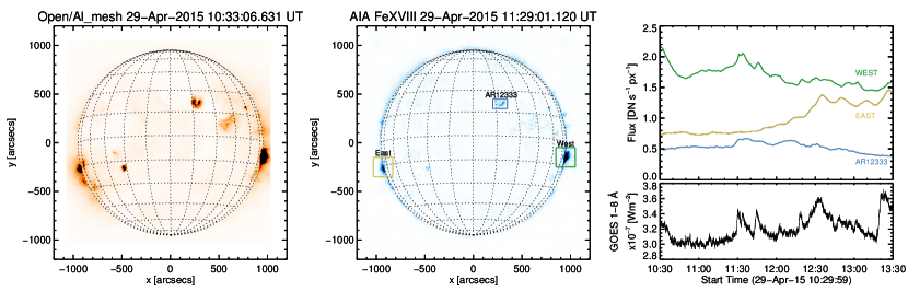
Figure 1: Overview of the SDO/AIA 94Å Fe XVIII conditions during the times of the NuSTAR observations, and Hinode/XRT prior to the AR12333 microflare onset. (Left) full-disk image from Hinode/XRT one hour prior to the microflare onset. (Middle) full-disk SDO/AIA 94Å Fe XVIII image at the peak of the microflare impulsive phase with the ARs indicated. The SDO/AIA 94Å Fe XVIII light curves from these three regions are shown in comparison to the full-disk GOES 1-8Å SXR flux (right). All of the regions are producing several microflares during these times, but those from AR12333 are hidden in the GOES lightcurve as those from the two limb regions are brighter.

The microflare from AR12333 occurred during a time when there were two brighter ARs on the disk, as can be seen in Figure 1. Both of these ARs, on either limb, were producing microflares that dominate the overall GOES 1-8Å SXR light curve (Figure 1, right panels). GOES is spatially integrated, but the contributions from each region can be determined by using the hotter Fe XVIII component of SDO/AIA 94Å images. The Fe XVIII line contribution to the SDO/AIA 94Å channel peaks at $log_{10}T=6.85$ K ($\sim 7$ MK), and can be recovered using a combination of the SDO/AIA channels (Reale et al., 2011; Warren et al., 2012; Testa & Reale, 2012; Del Zanna, 2013). Here we use the approach of Del Zanna (2013)

$$\begin{split}F(\text{{Fe~{}XVIII}})\approx&~{}F(\text{94\AA})\\ &-\frac{F(\text{211\AA})}{120.}-\frac{F(\text{171\AA})}{450.},\end{split}$$ (1)

where $F(\text{{Fe~{}XVIII}})$ is the Fe XVIII flux [DN s^-1 px^-1] and $F(\text{94\AA})$, $F(\text{171\AA})$, $F(\text{211\AA})$, are the equivalent fluxes in the SDO/AIA 94Å, 171Å, and 211Å channels.

Hinode/XRT observed AR12333 in a high cadence mode ($\sim 2-3$ minutes), cycling through five different filter channels centered on this region. Full-disk synoptic images were obtained before and after this observation mode (Figure 1). Figure 2 shows the main loops of the region rapidly brightening, indicating that energy is being released to heat these loops. This is apparent in the SXR channels from Hinode/XRT and SDO/AIA 94Å Fe XVIII, but not the cooler EUV channels from SDO/AIA, so we conclude that the heating is mostly above $3$ MK. For the $95\arcsec\times 45\arcsec$ loop region shown in Figure 2 we produce the time profile of the microflares in each of these SXR and EUV channels, shown in Figure 3. These light curves have been obtained after processing via the instrument preparation routines, de-rotation of the solar disk (to $\sim$11:29 UT), and manual alignment of Hinode/XRT Be-Thin to the $1\arcsec$ down-sampled SDO/AIA 94Å Fe XVIII data. Here we again see that the microflare activity is only occurring in the channels sensitive to the hottest material, i.e. the SXR ones from Hinode/XRT and SDO/AIA 94Å Fe XVIII. This activity is in the form of three distinctive peaks with the first, and largest, impulsively starting at $\sim$ 11:29 UT. This is clear in the SXR (with the exception of the low signal-to-noise Hinode/XRT Be-Thick channel), and SDO/AIA 94Å Fe XVIII lightcurves, all showing similar time profiles.

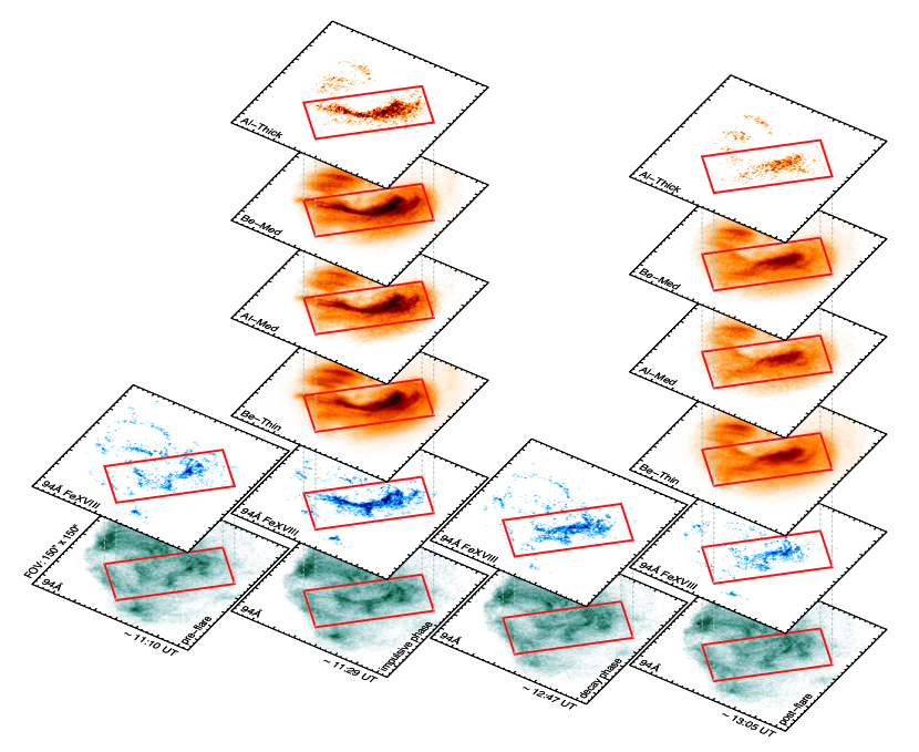
Figure 2: Comparison of AR12333 from SDO/AIA and Hinode/XRT at the times of NuSTAR observations (pre-flare, $\sim$ 11:10 UT; impulsive phase, $\sim$ 11:29 UT; decay phase, $\sim$ 12:47 UT; and post-flare, $\sim$ 13:05 UT). The loop region ($95\arcsec\times 45\arcsec$) used for the light curves and DEM analysis is over plotted as a red rectangle. The loop region is faintly observable in SDO/AIA 94Å with the structure well-recovered in the SDO/AIA 94Å Fe XVIII and SXR channels.

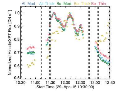
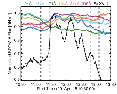
Figure 3: Time profiles of the different Hinode/XRT (top) and SDO/AIA (bottom) channels from the loop region of AR12333 shown in Figure 2. The vertical bars indicate the four time periods of the NuSTAR observation of the same region. The gaps in the Hinode/XRT light curves are due to incomplete coverage.

3 NuSTAR Data Analysis

NuSTAR is an imaging spectrometer with high sensitivity to X-rays over $2.5$ to $78$ keV (Harrison et al., 2013). NuSTAR consists of two identical telescopes each with the same $12\arcmin\times 12\arcmin$ field of view (Madsen et al., 2015) and is composed of Wolter-I type optics that directly focus X-rays onto the focal-plane modules (FPMA and FPMB) $10$ m behind. These focal-plane modules each comprise of CdZnTe detectors with $64\times 64$ pixels providing the time, energy, and location of the incoming X-rays. The readout time per event is 2.5 ms, and NuSTAR accepts a maximum throughput of $400$ counts s^-1 for each focal-plane module. This makes NuSTAR highly capable of observing weak thermal or non-thermal X-ray sources from the Sun (Grefenstette et al., 2016). However, as it is optimised for astrophysics targets solar pointings have limitations. In particular, the low detector readout and large effective area produce high detector deadtime even for modest levels of solar activity, restricting the spectral dynamic range, only detecting X-rays at the lowest energies (Hannah et al., 2016; Grefenstette et al., 2016). NuSTAR solar observations are therefore from times of weak solar activity, ideally when the GOES $1-8$Å  flux is below B-level. An overview of the initial NuSTAR solar pointings, that began in late 2014, and details of these restrictions is available in Grefenstette et al. (2016). An up-to-date quicklook summary is also available online.

The observations reported here are based around the fourth NuSTAR solar pointing, consisting of two orbits of observations covering 2015 April 29 10:50 to 11:50 and 12:27 to 13:27 (Grefenstette et al., 2016). NuSTAR completed a full disk mosaic observation in each orbit consisting of 17 different pointings: the field of view requires 16 different pointings to cover the whole Sun, with some overlaps between each mosaic tile, followed by an additional disk centre pointing (see Figure 4 Grefenstette et al., 2016). This resulted in NuSTAR observing AR12333 four times, each lasting for a few minutes. These times are shown in Figure 3. These data were processed using the NuSTAR Data Analysis software v1.6.0 and NuSTAR CALDB 20160502, which produces an event list for each pointing. We use only single-pixel (“Grade 0”) events (Grefenstette et al., 2016), to minimize the effects of pile-up. Figure 4 shows the resulting NuSTAR $2.5-4.5$ keV image for each of the four pointings and these images are a combination of both FPMA and FPMB with $\sim$7$\arcsec$ Gaussian smoothing as the pixel size is less than the full width at half maximum (FWHM) of the optics.

Two of these pointings, the first and last, caught the whole AR but the other two only caught the lower part as they were observed at the edge of the detector, however this is the location of the heated loops during the microflares in Figure 2. During some of the observations there was a change in the combination of Camera Head Units (CHUs) – star trackers used to provide pointing information. In those such instances we used the time range that gave the longest continuous CHU combination, instead of the whole duration. Each required a different shift to match the SDO/AIA 94Å Fe XVIII map at that time, and all were within the expected 1′ offset (Grefenstette et al., 2016). The alignment was straightforward for the NuSTAR maps which caught the whole region but was trickier for those with a partial observation. In those cases, second and third pointings, emission from another region (slightly to the south-west of AR12333) was used for the alignment. The resulting overlap of the aligned Hinode/XRT and NuSTAR images to SDO/AIA 94Å Fe XVIII are shown in Figure 5. The NuSTAR maps in Figure 4 reveal a similar pattern to the heating seen in EUV and SXR with SDO/AIA and Hinode/XRT: emission from the whole region before the microflare, with loops in the bottom right brightening as material is heated during the microflare, before fading as the material cools.

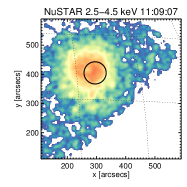
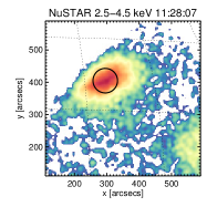
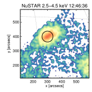
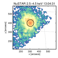
Figure 4: NuSTAR $2.5-4.5$ keV maps for the four time intervals it observed AR12333. These maps have been shifted to match the position of the SDO/AIA 94Å Fe XVIII maps, shown in Figure 5. The black circles indicate the regions chosen for spectral fitting, shown in Figure 6. Note that the same colour scaling is used in all these maps.

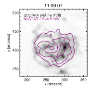
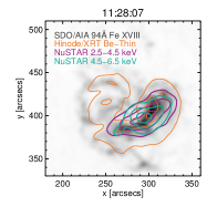
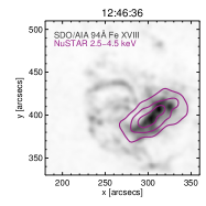
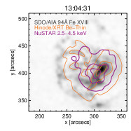
Figure 5: SDO/AIA 94Å Fe XVIII maps over plotted with shifted contours from Hinode/XRT (20%, 50%, 80%; orange), and NuSTAR $2.5-4.5$ keV and $4.5-6.5$ keV emission (50%, 70%, 90%; purple, turquoise). A constant offset correction was required for Hinode/XRT but a different one was determined for each NuSTAR pointing. For the two time intervals where NuSTAR only observed part of the AR (middle two panels), the alignment was done using the full map and to other features on the disk.

3.1 NuSTAR Spectral Fitting

For each of the NuSTAR pointings we chose a region at the same location, and of the same area, as those used in the SDO/AIA and Hinode/XRT analysis, to produce spectra of the microflare heating. These are circular as the NuSTAR software can only calculate the response files for such regions, but do cover the flaring loop region (rectangular box, Figure 2), and are shown in Figure 4. The spectra and NuSTAR response files were obtained using the NuSTAR Data Analysis software v1.6.0. These were then fitted using the XSPEC (Arnaud, 1996) software, which simultaneously fits the spectra from each telescope module (FPMA and FPMB) instead of just adding the data sets. We also use XSPEC as it allows us to find the best-fit solution using Cash statistics (Cash, 1979) which helps with the non-Gaussian uncertainties we have for the few counts at higher temperatures.

We fitted the spectra with a single thermal model, using the APEC model with solar coronal abundances (Feldman et al., 1992), and the fit results are shown in Figure 6. For the first and fourth NuSTAR pointings, before and after the microflares, the spectra are well fitted by this single thermal model showing similar temperatures and emission measures ($3.3$ MK and $6.3\times 10^{46}$ cm^-3, then $3.2$ MK and $7.0\times 10^{46}$ cm^-3). Above $5$ keV there are very few counts and this is due to a combination of the low livetime of the observations (164s and 152s dwell time with about 2% livetime fraction resulting in effective exposures of around 3.5s) and the high likelihood that the emission from this region peaked at this temperature before falling off very sharply at higher temperatures. These temperatures are similar to the quiescent ARs previously studied by NuSTAR (Hannah et al., 2016), although those regions were brighter and more numerous in the field of view, resulting in an order-of-magnitude worse livetime. The low livetime has the effect of limiting the spectral dynamic range, putting most of detected counts at the lower energy range, and no background or source counts at higher energies (Hannah et al., 2016; Grefenstette et al., 2016).

The two NuSTAR spectra from during the microflare, the second (impulsive phase) and third (decay phase, weaker peak) both show counts above $5$ keV and produce higher temperature fits ($5.1$ MK and $3.5$ MK). This is expected as there should be heating during the microflare, but neither fit matches the observed spectrum well, particularly during the impulsive phase. This shows that there is additional hot material during these times that a single-component thermal model cannot accurately characterise. For the spectrum during the impulsive phase, the second NuSTAR pointing, we tried adding additional thermal components to the fit, shown in Figure 7. We started by adding in a second thermal component fixed with the parameters from the pre-microflare spectrum, found from the first NuSTAR pointing (left spectrum in Figure 6), to represent the background emission. We did this as NuSTAR’s pointing changed during these two times (changing the part of the detector observing the region, and hence instrumental response) so we could not simply subtract the data from this pre-flare background time. The other thermal model component was allowed to vary and produced a slightly better fit to the higher energies and a higher temperature ($5.6$ MK). However this model still misses out counts at higher energies.

So we tried another fit where the two thermal models were both allowed to vary and this is shown in the right of Figure 7. Here there is a substantially better fit to the data over the whole energy range, fitting a model of $4.1$ MK and $10.0$ MK. The hotter model does seem to match the bump in emission between $6$ and $7$ keV, which at these temperatures would be due to line emission from the Fe K-Shell transition (Phillips, 2004). Although this model better matches the data, it produces substantial uncertainties, particularly in the emission measure. This is because it is fitting the few counts at higher energies which have a poor signal to noise. It should be noted that for the thermal model the temperature and emission measure are correlated and so the upper uncertainty on the temperature relates to the lower uncertainty on the emission measure, and vice versa. Therefore this uncertainty range covers a narrow diagonal region of parameter space, which we include later in Figure 11. These fits do however seem to indicate that emission from material up to $10$ MK is present in this microflare and that the NuSTAR spectrum in this case is observing purely thermal emission. A non-thermal component could still be present, but the likely weak emission, combined with NuSTAR’s low livetime (limiting the spectral dynamic range), leaves this component hidden. Upper-limits to this possible non-thermal emission are calculated in §5.2.

From these spectral fits we estimated the GOES $1-8$ Å flux to be $5.3\times 10^{-9}$ Wm^-2 for the impulsive phase, and $4.0\times 10^{-9}$ Wm^-2 for the pre-flare time. This means that the background subtracted GOES class for the impulsive phase is equivalent to $\sim$A0.1 and would be slightly larger during the subsequent peak emission time.

4 Multi-thermal Microflare Emission

The NuSTAR spectrum during the impulsive phase of the microflare clearly shows that there is a range of heated material, so to get a comprehensive view of this multi-thermal emission we recovered the differential emission measure (DEM) by combining the observations from NuSTAR, Hinode/XRT, and SDO/AIA. This is the first time these instruments have been used together to obtain a DEM.

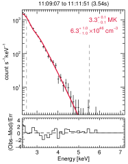
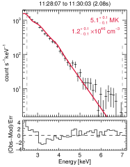
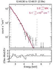
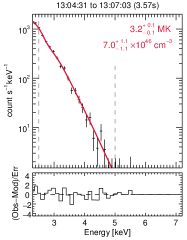
Figure 6: NuSTAR spectra for the regions shown in Figure 5, at different stages of flare evolution with time, increasing from left to right. The black data points show the combined data from FPMA and FPMB, and the red line shows the best fit thermal model. Note that the fit was performed to the data simultaneously and is only combined for plotting. The bottom panels show the residuals and the dashed vertical grey lines indicate the energy range over which the fit was performed (starting from the minimal usable energy of $2.5$ keV up where there are still substantial counts). The quoted uncertainties are with 90% confidence.

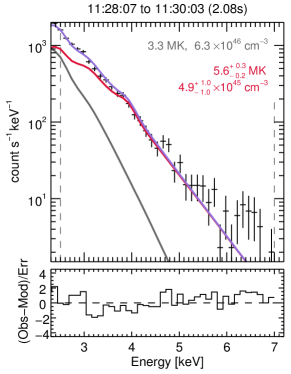
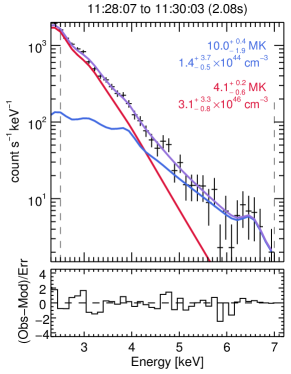
Figure 7: Additional model fits to the NuSTAR spectrum for the impulsive phase of the microflare. (Left) model of two thermals, one fixed using the parameters from the pre-flare observation (grey line), the second one (red) fitted. (Right) Model fitting two thermals. In both cases the total model is shown by the purple line and the black data points show the combined data from FPMA and FPMB. Note that the fit was performed to the data simultaneously and is only combined for plotting here. The quoted uncertainties are 90% confidence levels.

4.1 Comparison of NuSTAR, Hinode/XRT & SDO/AIA

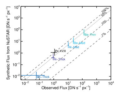
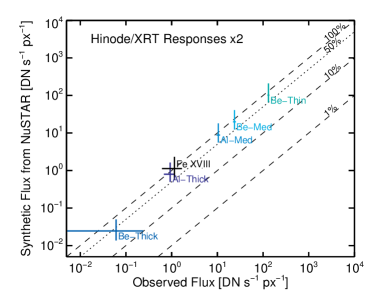
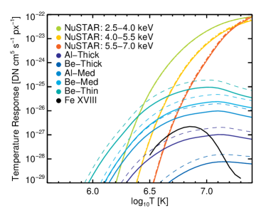
Figure 8: (Top) Comparison of Hinode/XRT and SDO/AIA 94Å Fe XVIII fluxes during the microflare’s impulsive phase, to the synthetic values obtained from the NuSTAR spectral fit. (Bottom) The temperature response functions for NuSTAR (FPMA, solid; FPMB, dot-dash) for the region shown in Figure 4 (panel 2), SDO/AIA 94Å Fe XVIII (solid black), and Hinode/XRT (original, solid; $\times 2$, dashed). This has been done using the standard Hinode/XRT responses (top left) and then multiplying them by a factor of two (top right) which gives values closer to the observed fluxes.

To check the compatibility of the NuSTAR, Hinode/XRT, and SDO/AIA observations we compared the observed fluxes from Hinode/XRT, and SDO/AIA to synthetic fluxes obtained from the NuSTAR thermal fits. For the NuSTAR two thermal fit (Figure 7, right panel) we multiplied the emission measures by the SDO/AIA and Hinode/XRT temperature response functions at the corresponding temperatures, and then added the two fluxes together to get a value for each filter channel.

The Hinode/XRT temperature response functions were created using xrt_flux.pro with a CHIANTI 7.1.3 (Dere et al., 1997; Landi et al., 2013) spectrum (xrt_flux713.pro) with coronal abundances (Feldman et al., 1992), and the latest filter calibrations that account for the time-dependent contamination layer present on the CCD (Narukage et al., 2014). The SDO/AIA temperature response functions are version six (v6; using CHIANTI 7.1.3) and obtained using aia_get_response.pro with the ‘chiantifix’, ‘eve_norm’, and ‘timedepend_date’ flags. The comparison of the observed and synthetic fluxes are shown in Figure 8.

We found that the SDO/AIA 94Å Fe XVIII synthetic flux is near the observed value, as expected, however there is a consistent discrepancy for Hinode/XRT. The observed fluxes should match the synthetic fluxes from the NuSTAR spectral fits as they are sensitive to the same temperature range. Other authors have found similar discrepancies (Testa et al., 2011; Cheung et al., 2015; Schmelz et al., 2015) and there is the suggestion that the Hinode/XRT temperature response functions are too small by a factor of $\sim 2-3$ (see Schmelz et al., 2015). We have therefore multiplied the Hinode/XRT temperature response functions by a factor of two (Figure 8, top right) and find a closer match to the synthetic values derived from the NuSTAR spectral fits. The main effect of these larger temperature response functions is that it requires there to be weaker emission at higher temperatures to obtain the same Hinode/XRT flux.

4.2 Differential Emission Measure

Recovering the line-of-sight DEM, $\xi(T_{j})$, involves solving the ill-posed inverse problem, ${g}_{i}={\bf K}_{i,j}\xi(T)$, where $g_{i}$ [DN s^-1 px^-1] is the observable, and ${\bf K}_{i,j}$ is the the temperature response function for the $ith$ filter channel, and the $jth$ temperature bin. Numerous algorithms have been developed for the DEM reconstruction, and we use two methods to recover the DEM: Regularised Inversion (RI, Hannah & Kontar, 2012), and the xrt_dem_iterative2.pro method (XIT, Golub et al., 2004; Weber et al., 2004).

The regularised inversion (RI) approach recovers the DEM by limiting the amplification of uncertainties using linear constraints. Uncertainties on the DEM are also found on both the DEM and temperature resolution (horizontal uncertainties), see Hannah & Kontar (2012). XIT is a forward-fitting iterative least-squares approach, using a spline model. Uncertainties in the final DEM are calculated with Monte Carlo (MC) iterations with input data perturbed by an amount randomly drawn from a Gaussian distribution with the standard deviation equal to the uncertainty in the observation. The resulting spread of these MC iterations indicates the goodness-of-fit.

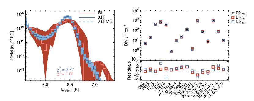
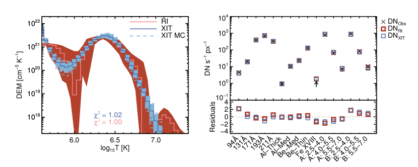
Figure 9: (Left) DEMs obtained during the impulsive phase of the microflare using SDO/AIA, Hinode/XRT and NuSTAR data. (Right) Residuals of the DEMs in data-space. The pink DEM (red error region) was obtained using the RI, and the blue (with 300 sky blue MC iterations) from XIT. The DEMs were calculated using both the standard Hinode/XRT temperature responses (top) as well as those multiplied by a factor of two (bottom).

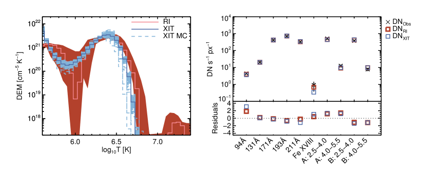
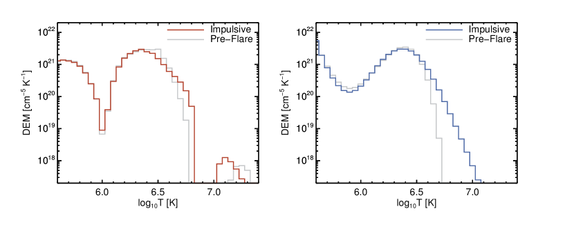
Figure 10: (Top Left) DEM obtained from the pre-flare phase ($\sim$ 11:10 UT) using SDO/AIA, and NuSTAR data. (Top Right) Residuals of the DEMs in data-space. (Bottom) The RI (left) and XIT (right) pre-flare DEMs shown in comparison to the impulsive-phase DEMs (Figure 9, bottom row). The pre-flare DEMs peak at similar temperatures, and fall off more steeply than the impulsive-phase DEMs. The increase in the DEMs is due to the heating during the microflare.

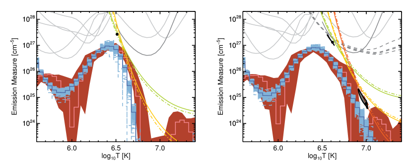
Figure 11: Emission measure distribution obtained from the pre-flare (left) using SDO/AIA, and NuSTAR data, and the impulsive phase of the microflare (right) using SDO/AIA, Hinode/XRT and NuSTAR data with the Hinode/XRT responses multiplied by a factor of two. The EM loci curves for NuSTAR are shown in the same colours as in Figure 8; the SDO/AIA loci are plotted in grey, with 94Å Fe XVIII in dark grey; and Hinode/XRT loci are over plotted as dark grey dashed lines. The thermal fits from Figures 6 and 7 are plotted as filled circles (black) with shaded 90% confidence contours.

For the DEM analysis we calculated the uncertainties on the Hinode/XRT and SDO/AIA data. The non-statistical photometric uncertainties for Hinode/XRT were calculated from xrt_prep.pro (Kobelski et al., 2014), and photon statistics calculated from xrt_cvfact.pro (Narukage et al., 2011, 2014). The uncertainties on the SDO/AIA data were computed with aia_bp_estimate_error.pro (Boerner et al., 2012), and an additional 5% systematic uncertainty was added in quadrature to both the Hinode/XRT and SDO/AIA data account for uncertainties in the temperature response functions. The Hinode/XRT and SDO/AIA data and uncertainties have been interpolated to a common time-step, and averaged over the NuSTAR observational duration. The uncertainty for the NuSTAR values in specific energy bands were determined as a combination of the photon shot noise and a systematic factor (of 5%) to account for the cross-calibration between NuSTAR’s two telescope modules (FPMA and FPMB). The NuSTAR temperature response functions, for each energy range and telescope module (shown in Figure 8) were calculated using the instrumental response matrix for the regions shown in Figure 4.

The resulting DEMs obtained for the impulsive phase are shown in Figure 9 (left) with the quality of the recovered DEM solution shown as residuals between the input, and recovered fluxes (right). XIT is used with the addition of $300$ MC iterations where outlier XIT MC solutions have been omitted. We have used all available filters with the exception of Hinode/XRT Be-Thick due to large uncertainties that are the result of a lack of counts (Figure 3), and SDO/AIA 335Å due to the observed long-term drop in sensitivity (see Figure 1 Boerner et al., 2014). The standard Hinode/XRT responses (Figure 9, top) lead to disagreement between the two methods for DEM recovery, notably at the peak, and at higher temperatures ($\chi_{XIT}^{2}=2.77$, $\chi_{RI}^{2}=1.01$). Using the Hinode/XRT responses multiplied by a factor of two results in the methods having much better agreement ($\chi_{XIT}^{2}=1.02$, $\chi_{RI}^{2}=1.00$), and the DEM solutions result in smaller residuals, specifically in the Hinode/XRT filters. These final DEMs (Figure 9, bottom) show a peak at $\sim 3$ MK, and little material above $10$ MK.

To understand how much of this material has been heated out of the background during the microflare we performed DEM analysis for the pre-flare NuSTAR time ($\sim$ 11:10 UT). There is no Hinode/XRT data for this time so we determined the DEM using NuSTAR and SDO/AIA data. The DEMs for the pre-flare observations are shown in Figure 10. These DEMs for each method peak at a similar temperature ($\sim 3$ MK), and fall off very sharply to $\sim 5$ MK. During the microflare there is a clear addition of material up to $10$ MK (Figure 10, bottom).

We also represent the DEMs as the emission measure distributions (EMDs; $\xi(T)\text{d}T$) which allows us to compare the DEM results to the NuSTAR spectral fits, shown in Figure 11. Here we have also over plotted the EM loci curves, $EM_{i}=g_{i}/K_{i}$, which are the upper-limits of emission based on an isothermal model, with the true solution lying below all of the EM loci curves. The NuSTAR thermal model fits are the isothermal (in the pre-flare phase) or two thermal (impulsive phase) fits to the multi-thermal plasma distribution, and so represent an approximation of the temperature distribution and emission measure. These models produce the expected higher emission measure values compared to the EMD, and are consistent with the EM loci curves.

5 Microflare Energetics

5.1 Thermal Energy

For an isothermal plasma at a temperature T and emission measure EM, the thermal energy is calculated as

$$U_{T_{I}}=3k_{B}T\sqrt{EMfV}\quad\text{[erg]}$$ (2)

where $k_{B}$ is the Boltzmann constant, f, the filling factor, and V, the plasma volume (e.g. Hannah et al., 2008). Using the two thermal fit (Figure 7, right) we calculated the thermal energy during the impulsive phase, finding $U_{T_{I}}=0.9\times 10^{28}$ erg ($t_{I}=116$ s). Here the equivalent loop volume, $V_{E}=fV$, was calculated as a volume of a cylinder enclosing only the flaring loop with length, L $\sim 50\arcsec$, and diameter, d $\sim 6\arcsec$. This thermal energy includes both the microflare and background emission. We found the pre-flare energy (using fit parameters; Figure 6, left) as $U_{T_{I_{0}}}=0.9\times 10^{28}$ erg (and $t_{{I}_{0}}=164$s). The resulting heating power during the microflare from the thermal fits to the NuSTAR spectra is then $P_{T_{I_{F}}}=U_{T_{I}}/t_{I}-U_{T_{I_{0}}}/t_{{I}_{0}}=2.5\times 10^{25}$ erg s^-1.

The thermal energy can also be estimated for a multi-thermal plasma using

$$U_{T}=3k_{B}V_{E}^{1/2}\frac{\int_{T}{T\xi_{V}(T)~{}dT}}{\sqrt{\int_{T}{\xi_{V}(T)~{}dT}}}\quad\text{[erg]}$$ (3)

as described in Inglis & Christe (2014), with the filling factor, $f=1$, and $\xi_{V}(T)=n^{2}\mathrm{d}V/\mathrm{d}T$ in units of cm^-3 K^-1. For the RI and XIT DEM solutions we find values of $U_{T_{RI}}=1.1\times 10^{28}$ erg, and $U_{T_{XIT}}=1.2\times 10^{28}$ erg during the impulsive phase of the microflare. The pre-flare thermal energies we find $U_{T_{RI_{0}}}=1.2\times 10^{28}$ erg, and $U_{T_{XIT_{0}}}=1.2\times 10^{28}$ erg, and this then gives values of the heating power during the impulsive phase of the microflare as $P_{T_{RI_{F}}}=2.3\times 10^{25}$ erg s^-1, and $P_{T_{XIT_{F}}}=3.0\times 10^{25}$ erg s^-1. All of these approaches give a similar value for the heating, about $2.5\times 10^{25}$ erg s^-1, over the microflare’s impulsive period, and a summary of these values with uncertanties are given in Table 1. It should be noted that these values are lower limits as the estimates neglect losses during heating.

Table 1: Summary of thermal energies of AR12333.

Method	$U_{T_{0}}\tablenotemark{a}$	$U_{T}\tablenotemark{b}$	$P_{T_{F}}$
	[$\times 10^{28}$ erg]	[$\times 10^{28}$ erg]	[$\times 10^{25}$ erg s-1]
NuSTAR fit	$0.9^{+0.1}_{-0.1}$	$0.9^{+0.6}_{-0.2}$	$2.5^{+5.4}_{-1.6}$
RI	$1.2^{+0.1}_{-0.1}$	$1.1^{+0.1}_{-0.1}$	$2.3^{+0.9}_{-1.0}$
XIT	$1.2^{+0.1}_{-0.1}$	$1.2^{+0.1}_{-0.1}$	$3.0^{+0.6}_{-0.7}$

Note. — The uncertainties on the energies and power derived from the NuSTAR fit are $2.7\sigma$ (90% confidence), and those from RI/XIT are $1\sigma$.

From the analysis of $25,705$ RHESSI events, (Table 1 Hannah et al., 2008) microflare thermal energies were found to range from $U_{T}=10^{26-30}$ erg ($5\%-95\%$ range; from a $16$s observation). This is equivalent to $P_{T}=6.3\times 10^{24-28}$ erg s^-1, and therefore the thermal power from our NuSTAR microflare is in the lower range of RHESSI observations. This is as expected as NuSTAR should be able to observe well beyond RHESSI’s sensitivity limit to small microflares.

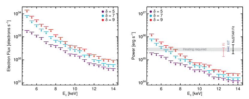
Figure 12: Non-thermal upper-limits as a function of $E_{c}$ and $\delta$ plotted in terms of non-thermal electron flux, $N_{N}$ (left), and non-thermal power, $P_{N}$ (right). The three estimates for the thermal power: $P_{T_{I_{F}}}$, black; $P_{T_{RI_{F}}}$, pink; and $P_{T_{XIT_{F}}}$, blue, are plotted with $1\sigma$ uncertainties. The grey shaded region represents the required heating power, consistent with all three estimates.

5.2 NuSTAR Non-thermal Limits

As the NuSTAR spectrum in Figure 7 is well fitted by a purely thermal model we can therefore find the upper-limits of the possible non-thermal emission. This approach allows us to determine whether the accelerated electrons could power the observed heating in this microflare. We used the thick-target model of a power-law electron distribution above a low-energy cut-off E_c [keV] given by

$$F(E>E_{c})\propto E^{-\delta}$$ (4)

where $\delta$ is the power-law index, and the power in this non-thermal distribution is given by

$$P_{N}(>E_{c})=1.6\times 10^{-9}\frac{\delta-1}{\delta-2}N_{N}E_{c}\quad\text{[erg s}^{-1}\text{]}$$ (5)

where $N_{N}$ is the non-thermal electron flux [electrons s^-1].

We determined the upper-limits on $N_{N}$ (and $P_{N}$) for a set of $\delta$ ($\delta=5,7,9$), and $E_{c}$ consistent with a null detection in the NuSTAR spectrum. We performed this by iteratively reducing the model electron flux $N_{N}$ until there were less than 4 counts $>7$ keV, consistent with a null detection to $2\sigma$ (Gehrels, 1986). We also ensured the number of counts $\leq 7$ keV are within the counting statistics of the observed counts. For each iteration we generated the X-ray spectrum for the two-component fitted thermal model (Figure 7, right) and added to this the non-thermal X-ray spectrum for our chosen $\delta$, $E_{c}$, and $N_{N}$, calculated using f_thick2.pro (see Holman et al., 2011). This was then folded through the NuSTAR response to generate a synthetic spectrum (as discussed in Hannah et al., 2016). The upper-limits are shown in Figure 12 along with the three estimates of the thermal power for the background-subtracted flare, $P_{T_{I_{F}}}$ (“NuSTAR Fit”, black), $P_{T_{RI_{F}}}$ (pink), and $P_{T_{XIT_{F}}}$ (blue). For a flatter spectrum of $\delta=5$ barely any of the upper-limits are consistent with the required heating power. With a steeper spectrum, $\delta\geq 7$, a cut-off $E_{c}\lesssim 7$ keV is consistent with the heating requirement. These steep spectra indicate that the bulk of the non-thermal emission would need to be at energies close to the low energy cut-off to be consistent with the observed NuSTAR spectrum. If we instead consider some of the counts in the $6-7$ keV range to be non-thermal (e.g. the excess above thermal model in the left panel in Figure 7) then we would obtain higher non-thermal power, about a factor of $0.5$ larger. However this would only substantially effect the steep non-thermal spectra ($\delta\geq 7$) as flatter models would be inconsistent with the data below $7$ keV.

We can again compare the microflare studied here to non-thermal energetics derived from RHESSI microflare statistics. Hannah et al. (2008) report non-thermal parameters of $\delta=4-10$, $E_{c}=9-16$ keV, and the non-thermal power ranges from $P_{N}(\geq E_{c})=10^{25-28}$ erg s^-1. The largest upper-limits NuSTAR produces for this microflare are again at the the edge of RHESSI’s sensitivity. In a previous study of nanoflare heating Testa et al. (2014) investigated the evolution of chromospheric and transition region plasma from IRIS observations using RADYN nanoflare simulations. This is one of the few non-thermal nanoflare studies and they reported that heating occurred on time-scales of $\lesssim 30$s characterized by a total energy $\lesssim 10^{25}$ erg, and $E_{c}\sim 10$ keV. The simulated electron beam parameters in this IRIS event are consistent with the NuSTAR derived parameters, but in a range insufficient to power the heating in our microflare.

6 Discussion and Conclusions

In this paper we have presented the first joint observations of a microflaring AR with NuSTAR, Hinode/XRT, and SDO/AIA. During the impulsive start, the NuSTAR spectrum shows emission up to $10$ MK, indicating that even in this $\sim$A0.1 microflare substantial heating can occur. This high temperature emission is confirmed when we recover DEMs using the NuSTAR, Hinode/XRT, and SDO/AIA data. These instruments crucially overlap in temperature sensitivity, with NuSTAR able to constrain and characterise the high temperature emission which is often difficult for other instruments to do alone.

In this event we find the Hinode/XRT temperature response functions are a factor of two too small, suggesting that it would normaly overestimate the contribution from high temperature plasma in this microflare.

Overall we find the instantaneous thermal energy during the microflare to be $\sim 10^{28}$ erg, once the pre-flare has been subtracted this equates to a heating rate of $\sim 2.5\times 10^{25}$ erg s^-1 during the impulsive phase of this microflare. This is comparable to some of the smallest events observed with RHESSI, although RHESSI did not see this microflare as its indirect imaging was dominated by the brighter ARs elsewhere on the disk.

Although no non-thermal emission was detected, we can place upper-limits on the possible non-thermal component. We find that we would need a steep ($\delta\geq 7$) power-law down to at least $7$ keV to be able to power the heating in this microflare. This is still consistent with this small microflare being physically similar to large microflares and flares, but this would only be confirmed if NuSTAR detected non-thermal emission. To achieve this, future NuSTAR observations need to be made with a higher effective exposure time. For impulsive flares this cannot be achieved with longer duration observations, but only with higher livetimes. Observing the Sun when there are weaker or fewer ARs on the disk would easily achieve this livetime increase, conditions that have occurred since this observation and will continue through solar minimum.

These observations would greatly benefit from new, more sensitive, solar X-ray telescopes such as the FOXSI (Krucker et al., 2014) and MaGIXS (Kobayashi et al., 2011) sounding rockets, as well as the MinXSS CubeSats (Mason et al., 2016). New data combined with NuSTAR observations during quieter periods of solar activity should provide detection of the high-temperature and possible non-thermal emission in even smaller microflares which should, in turn, provide a robust measure of their contribution to heating coronal loops in ARs.

References

- Arnaud (1996) Arnaud, K. A. 1996, in Astronomical Society of the Pacific Conference Series, Vol. 101, Astronomical Data Analysis Software and Systems V, ed. G. H. Jacoby & J. Barnes, 17
- Aschwanden et al. (2000) Aschwanden, M. J., Tarbell, T. D., Nightingale, R. W., et al. 2000, ApJ, 535, 1047
- Boerner et al. (2012) Boerner, P., Edwards, C., Lemen, J., et al. 2012, Sol. Phys., 275, 41
- Boerner et al. (2014) Boerner, P. F., Testa, P., Warren, H., Weber, M. A., & Schrijver, C. J. 2014, Sol. Phys., 289, 2377
- Cash (1979) Cash, W. 1979, ApJ, 228, 939
- Cheung et al. (2015) Cheung, M. C. M., Boerner, P., Schrijver, C. J., et al. 2015, ApJ, 807, 143
- Christe et al. (2008) Christe, S., Hannah, I. G., Krucker, S., McTiernan, J., & Lin, R. P. 2008, ApJ, 677, 1385
- Del Zanna (2013) Del Zanna, G. 2013, A&A, 558, A73
- Dere et al. (1997) Dere, K. P., Landi, E., Mason, H. E., Monsignori Fossi, B. C., & Young, P. R. 1997, A&AS, 125, 149
- Feldman et al. (1992) Feldman, U., Mandelbaum, P., Seely, J. F., Doschek, G. A., & Gursky, H. 1992, ApJS, 81, 387
- Gburek et al. (2011) Gburek, S., Sylwester, J., Kowalinski, M., et al. 2011, Solar System Research, 45, 189
- Gehrels (1986) Gehrels, N. 1986, ApJ, 303, 336
- Glencross (1975) Glencross, W. M. 1975, ApJ, 199, L53
- Glesener et al. (2017) Glesener, L., Krucker, S., Hannah, I. G., et al. 2017, ApJ, in revision
- Golub et al. (2004) Golub, L., Deluca, E. E., Sette, A., & Weber, M. 2004, in Astronomical Society of the Pacific Conference Series, Vol. 325, The Solar-B Mission and the Forefront of Solar Physics, ed. T. Sakurai & T. Sekii, 217
- Golub et al. (2007) Golub, L., Deluca, E., Austin, G., et al. 2007, Solar Physics, 243, 63
- Grefenstette et al. (2016) Grefenstette, B. W., Glesener, L., Krucker, S., et al. 2016, ApJ, 826, 20
- Hannah et al. (2008) Hannah, I. G., Christe, S., Krucker, S., et al. 2008, ApJ, 677, 704
- Hannah et al. (2011) Hannah, I. G., Hudson, H. S., Battaglia, M., et al. 2011, Space Sci. Rev., 159, 263
- Hannah & Kontar (2012) Hannah, I. G., & Kontar, E. P. 2012, A&A, 539, A146
- Hannah et al. (2016) Hannah, I. G., Grefenstette, B. W., Smith, D. M., et al. 2016, ApJ, 820, L14
- Harrison et al. (2013) Harrison, F. A., Craig, W. W., Christensen, F. E., et al. 2013, ApJ, 770, 103
- Holman et al. (2011) Holman, G. D., Aschwanden, M. J., Aurass, H., et al. 2011, Space Sci. Rev., 159, 107
- Hudson (1991) Hudson, H. S. 1991, Sol. Phys., 133, 357
- Inglis & Christe (2014) Inglis, A. R., & Christe, S. 2014, ApJ, 789, 116
- Kobayashi et al. (2011) Kobayashi, K., Cirtain, J., Golub, L., et al. 2011, in Proc. SPIE, Vol. 8147, Society of Photo-Optical Instrumentation Engineers (SPIE) Conference Series, 81471M
- Kobelski et al. (2014) Kobelski, A. R., Saar, S. H., Weber, M. A., McKenzie, D. E., & Reeves, K. K. 2014, Sol. Phys., 289, 2781
- Kosugi et al. (2007) Kosugi, T., Matsuzaki, K., Sakao, T., et al. 2007, Sol. Phys., 243, 3
- Krucker et al. (1997) Krucker, S., Benz, A. O., Bastian, T. S., & Acton, L. W. 1997, ApJ, 488, 499
- Krucker et al. (2014) Krucker, S., Christe, S., Glesener, L., et al. 2014, ApJ, 793, L32
- Kuhar et al. (2017) Kuhar, M., Krucker, S., Hannah, I. G., et al. 2017, ApJ, 835, 6
- Landi et al. (2013) Landi, E., Young, P. R., Dere, K. P., Del Zanna, G., & Mason, H. E. 2013, ApJ, 763, 86
- Lemen et al. (2012) Lemen, J. R., Title, A. M., Akin, D. J., et al. 2012, Solar Physics, 275, 17
- Lin et al. (2002) Lin, R. P., Dennis, B. R., Hurford, G. J., et al. 2002, Sol. Phys., 210, 3
- Madsen et al. (2015) Madsen, K. K., Harrison, F. A., Markwardt, C. B., et al. 2015, The Astrophysical Journal Supplement Series, 220, 8
- Mason et al. (2016) Mason, J. P., Woods, T. N., Caspi, A., et al. 2016, Journal of Spacecraft and Rockets, 53, 328
- Narukage et al. (2014) Narukage, N., Sakao, T., Kano, R., et al. 2014, Sol. Phys., 289, 1029
- Narukage et al. (2011) —. 2011, Sol. Phys., 269, 169
- Parker (1988) Parker, E. N. 1988, ApJ, 330, 474
- Parnell & Jupp (2000) Parnell, C. E., & Jupp, P. E. 2000, ApJ, 529, 554
- Pesnell et al. (2012) Pesnell, W. D., Thompson, B. J., & Chamberlin, P. C. 2012, Sol. Phys., 275, 3
- Phillips (2004) Phillips, K. J. H. 2004, ApJ, 605, 921
- Reale et al. (2011) Reale, F., Guarrasi, M., Testa, P., et al. 2011, ApJ, 736, L16
- Schmelz et al. (2015) Schmelz, J. T., Asgari-Targhi, M., Christian, G. M., Dhaliwal, R. S., & Pathak, S. 2015, ApJ, 806, 232
- Testa & Reale (2012) Testa, P., & Reale, F. 2012, ApJ, 750, L10
- Testa et al. (2011) Testa, P., Reale, F., Landi, E., DeLuca, E. E., & Kashyap, V. 2011, ApJ, 728, 30
- Testa et al. (2014) Testa, P., De Pontieu, B., Allred, J., et al. 2014, Science, 346, 1255724
- Warren et al. (2012) Warren, H. P., Winebarger, A. R., & Brooks, D. H. 2012, ApJ, 759, 141
- Weber et al. (2004) Weber, M. A., Deluca, E. E., Golub, L., & Sette, A. L. 2004, in IAU Symposium, Vol. 223, Multi-Wavelength Investigations of Solar Activity, ed. A. V. Stepanov, E. E. Benevolenskaya, & A. G. Kosovichev, 321–328