Orbiton-magnon interplay in the spin-orbital polarons of KCuF₃ and LaMnO₃

Abstract

We present a quasi-analytical solution of a spin-orbital model of KCuF₃, using the variational method for Green’s functions. By analyzing the spectra for different partial bosonic compositions as well as the full solution, we show that hole propagation needs both orbiton and magnon excitations to develop, but the orbitons dominate the picture. We further elucidate the role of the different bosons by analyzing the self-energies for simplified models, establishing that because of the nature of the spin-orbital ground state, magnons alone do not produce a full quasiparticle band, in contrast to orbitons. Finally, using the electron-hole transformation between the $e_{g}$ states of KCuF₃ and LaMnO₃ we suggest the qualitative scenario for photoemission experiments in LaMnO₃.

I Introduction

In compounds with intraorbital Coulomb interaction $U$ electrons localize and the ground state is determined by effective superexchange interactions. The properties of such systems doped by holes may be very different Imada M. and Tokura (1998). The hole propagation in a two-dimensional (2D) antiferromagnetic (AF) square lattice Lee et al. (2006) is promoted by quantum fluctuations and is controlled by the superexchange $J$ Martínez and Horsch (1991). In systems with orbital degrees of freedom the superexchange is of spin-orbital form Tokura and Nagaosa (2000); Kugel and Khomskii (1982); Feiner et al. (1997); *FOZ98; Feiner and Oleś (1999); Khaliullin and Maekawa (2000); Khaliullin et al. (2001); *Hor08; *Kha04; Oleś et al. (2005); Khaliullin (2005); Krüger et al. (2009); Wohlfeld et al. (2011); *Woh13; *Che15; Eremin et al. (2011); Corboz et al. (2012); Nasu and Ishihara (2013); *Nas15; Brzezicki et al. (2015); *Brz16; *Brz17. One finds then the whole plethora of different behaviors and the details of hole propagation depend on the type of $3d$ orbitals involved and on the system’s dimension van den Brink et al. (2000); Bała et al. (2001); Yin et al. (2001); Ishihara (2005); Daghofer et al. (2008); *Woh08; Wohlfeld et al. (2009); *Mona; Wróbel and Oleś (2010).

Perhaps the most complex situation arises in the $e_{g}$ orbital model where both the orbital superexchange van den Brink et al. (1999) and the kinetic energy, which does not conserve the orbital flavor Feiner and Oleś (2005), are radically different from those in the spin $t$-$J$ model Chao et al. (1977). In a ferromagnetic (FM) compound, the orbital interactions are Ising-like in a one-dimensional model Daghofer et al. (2004) but quantum fluctuations increase via 2D towards three-dimensional (3D) orbital model van den Brink et al. (1999). This is in contrast to the SU(2) symmetric interactions in the AF Heisenberg model Martínez and Horsch (1991). However, when the ground state is AF and spin excitations contribute as well, hole propagation is dominated by the orbital excitations Wohlfeld et al. (2009); *Mona and holes are quasi-localized. It is a challenging question to ask what happens when AF and alternating orbital (AO) order appear in orthogonal directions. It was suggested that a priori only one type of excitations, either magnons or orbitons, will control hole propagation in photoemission for LaMnO₃ Bała et al. (2001), but this was not verified until now.

The purpose of this paper is to study in a systematic way the electron (hole) propagation in the 3D spin-orbital model for KCuF₃ (LaMnO₃) at low temperature $T\to 0$. We construct the $t$-$J$-like Hamiltonian with both spin and $e_{g}$ orbital degrees of freedom and show that while orbitons dominate the picture, magnons are also important to explain the low-energy quasiparticle (QP). Such a QP state is a spin-orbital polaron, defined as a moving charge dressed by both spin and orbital excitations Wohlfeld et al. (2009); *Mona. This polaron is analogous to the spin polaron in the undoped cuprates Martínez and Horsch (1991); Chernyshev et al. (2000); Fleck et al. (2001); Wróbel et al. (2008); Mierzejewski et al. (2011). Surprisingly, in the present case magnons do not slow down the polaron considerably or make it incoherent.

The remaining of the paper is organized as follows. We introduce the spin-orbital model in Sec. II. In Sec. III we describe the variational method used to derive the spectral function from a systematic expansion in terms of bosons standing for orbiton or magnon excitations. Numerical results are presented and discussed in Sec. IV. The paper is summarized by the conclusions in Sec. V. We present also an Appendix with the analytic results obtained for a one-boson expansion.

II The spin-orbital model

We first discuss KCuF₃ which is conceptually easier, being a tetragonal system (cubic in the first approximation), with Cu($d^{9}$) ions placed in octahedral cages of fluorides. Their crystal field splits the $3d$ orbitals into low-lying $t_{2g}$ quenched states and active $e_{g}$ states. The model of the undoped system includes hopping $t$ along $\sigma$ bonds between $3z^{2}_{\gamma}-r^{2}$ orbitals, where $z_{\gamma}=x,y,z$ for the axis $\gamma=a,b,c$ Feiner and Oleś (2005). The orthogonal $(x^{2}-y^{2})$-type orbitals do not hybridize due to the symmetry of the underlying $p$-$d$ bonds. The superexchange Hamiltonian between Cu ions is derived from $d^{9}d^{9}\Leftrightarrow d^{8}d^{10}$ virtual charge excitations in the presence of large $U$ Oleś et al. (2000). Therefore, KCuF₃ is described by a quintessential spin-orbital model combining these two degrees of freedom in an essentially isotropic 3D system. For vanishing Hund’s exchange it simplifies to two terms,

$$H_{1} =(J/S^{2})\sum_{\langle ij\rangle\|\gamma}\left(\bm{{S}}_{i}\cdot\bm{{S}}_{j}+S^{2}\right)\left(\tau_{i}^{\gamma}\tau_{j}^{\gamma}+\tfrac{1}{4}\right),$$ (1a)

$$H_{2} =(J/2S^{2})\sum_{\langle ij\rangle\|\gamma}\left(\bm{{S}}_{i}\cdot\bm{{S}}_{j}-S^{2}\right)\left(\tau_{i}^{\gamma}+\tau_{j}^{\gamma}\right),$$ (1b)

where $J=t^{2}/U$, i.e., $J_{\rm Cu}=4t^{2}/U$ for $S=1/2$ spins. The $T=1/2$ orbital operators depend on the direction $\gamma$: $\tau^{a(b)}=-\frac{1}{2}(T^{z}\mp\sqrt{3}T^{x})$ and $\tau^{c}=T^{z}$, under the standard convention van den Brink et al. (1999) with $\lvert 3z^{2}-r^{2}\rangle\equiv\lvert z\rangle$, $\lvert x^{2}-y^{2}\rangle\equiv\lvert\bar{z}\rangle$.

Experimental data Lake et al. (2005); Paolasini et al. (2002); Caciuffo et al. (2002); Deisenhofer et al. (2008) as well as local spin density approximation (LSDA) and LSDA+$U$ calculations Binggeli and Altarelli (2004); Pavarini et al. (2008); Leonov et al. (2010), and the simulations of effective spin-orbital model at large $U$ (with finite Hund’s exchange $J_{H}$) find Oleś et al. (2000) that the ground state of KCuF₃ has broken symmetry with $A$-type AF ($A$-AF) and $C$-type AO ($C$-AO) order. Indeed, the energy is gained from $H_{1}$ (1a) when either $\langle\bm{{S}}_{i}\cdot\bm{{S}}_{j}\rangle>0$ and $\langle\tau_{i}^{\gamma}\tau_{j}^{\gamma}\rangle<\frac{1}{4}$, or $\langle\bm{{S}}_{i}\cdot\bm{{S}}_{j}\rangle<S^{2}$ and $\langle\tau_{i}^{\gamma}\tau_{j}^{\gamma}\rangle>0$, as predicted by the Goodenough-Kanamori rules Goodenough (1963); Kanamori (1959). While the latter occurs for AF bonds along the $c$ axis, the former stands for FM spin order in $ab$ planes favored by finite Hund’s exchange $J_{H}>0$.

An orbital crystal field $H_{z}=E_{z}\sum_{i}T_{i}^{z}$ is equivalent to an axial pressure along the $c$ axis. It controls the AO order with orbitals selected to minimize the energy Bała et al. (2001). For convenience we take the classical ground state $\lvert 0\rangle$ for $\langle H_{2}+H_{z}\rangle_{\mathrm{cl}}=0$ , implying that the orbitals $\{\lvert z\rangle,\lvert\bar{z}\rangle\}$ are degenerate and the occupied hole states in the AO state of KCuF₃ are van den Brink et al. (1999): $\lvert\pm\rangle=\frac{1}{\sqrt{2}}(\lvert z\rangle\pm\lvert\bar{z}\rangle)$.

We now build the Hamiltonian for an electron doped into $\lvert 0\rangle$. Let $d_{i,mn}^{{\dagger}}$ be creation operators for an electron at site ${i}$. If $m=n=0$, the electron is added to the $d^{9}$ ground state configuration, else it is added to the orbital-excited state if $n=1$ and/or to the spin-excited state if $m=1$. We decompose $d_{i,mn}^{{\dagger}}=f_{i}^{{\dagger}}a_{i}^{n}b_{i}^{m}$, where $f_{i}^{{\dagger}}$ is a fermion operator for the $d^{10}$ state, and $a_{i}$ and $b_{i}$ are boson operators for orbital and spin excitations. Following the same procedure, we find these additional terms when an electron is doped in the system:

$$\mathcal{T} =-\frac{t}{4}\sum_{\langle ij\rangle\perp c}(f_{i}^{{\dagger}}f_{j}+\mathrm{H.c.})=\sum_{\bm{{k}}}\epsilon_{\bm{{k}}}f_{\bm{{k}}}^{{\dagger}}f_{\bm{{k}}},$$ (2a)

$$\mathcal{V}_{\perp}^{t} =-\frac{t}{4}\sum_{i,\delta\perp c}\left[(2+\sqrt{3}e^{i\pi_{y}\delta}e^{i\bm{{Q}}\bm{{R}}_{i}})a_{i}^{{\dagger}}+a_{i}^{{\dagger}}a_{i+\delta}+\right.$$

$$\left.+(2-\sqrt{3}e^{i\pi_{y}\delta}e^{i\bm{{Q}}\bm{{R}}_{i}})a_{i+\delta}\right](1+b_{i}b_{i+\delta}^{{\dagger}})f_{i}^{{\dagger}}f_{i+\delta}+\mathrm{H.c.}$$

$$-\frac{t}{4}\sum_{\langle ij\rangle\perp c}b_{i}b_{j}^{{\dagger}}f_{i}^{{\dagger}}f_{j}+\mathrm{H.c.},$$ (2b)

$$\mathcal{V}_{\parallel}^{t} =-\frac{t}{2}\!\sum_{\langle ij\rangle\parallel c}(a_{i}-1)(a_{j}^{{\dagger}}-1)(b_{i}+b_{j}^{{\dagger}})f_{i}^{{\dagger}}f_{j}+\mathrm{H.c.},$$ (2c)

where $\epsilon_{\bm{{k}}}=-t(\cos k_{x}+\cos k_{y})/2$, $\bm{{Q}}=(\pi,\pi,0)$, and $\pi_{y}=(0,\pi,0)$, with the lattice constant $a=1$.

Free fermion propagation (2a) is allowed within the $ab$ planes — it does not modify the AO order van den Brink et al. (2000). Other processes which contribute to in-plane fermion hopping are accompanied by creation or removal of orbitons, as well as moving magnons around (if any are present) (2). In contrast, along the $c$ axis free fermion hopping is blocked by the AF spin order, thus a magnon (spin-flip excitation) always accompanies fermion hopping between planes; orbitons may also be involved, see Eq. (2c).

III Variational approximation

We use a well-established variational method Berciu (2006); Marchand et al. (2010); Berciu and Fehske (2011); Ebrahimnejad et al. (2016) to determine the one-electron Green’s function $G(\bm{{k}},\omega)=\langle\bm{{k}}\rvert\mathcal{G}(\omega)\lvert\bm{{k}}\rangle$, where $\mathcal{G}(\omega)=[\omega+i\eta-\mathcal{H}]^{-1}$ is the resolvent operator and $\lvert\bm{{k}}\rangle=f_{\bm{{k}}}^{{\dagger}}\lvert 0\rangle$ is a free electron state doped into $\lvert 0\rangle$. The Hamiltonian is divided into $\mathcal{H}_{0}=\mathcal{T}+\mathcal{H}_{J}^{z}$, with the Ising part of the exchange (1) (we have verified that the quantum fluctuations are of little importance and we ignore them, also see Bieniasz et al. (2016)), and the interaction $\mathcal{V}=\mathcal{V}_{\perp}^{t}+\mathcal{V}_{\parallel}^{t}$.

The variational method uses Dyson’s equation $\mathcal{G}(\omega)=\mathcal{G}_{0}(\omega)+\mathcal{G}(\omega)\mathcal{V}\mathcal{G}_{0}(\omega)$ to generate equations of motion (EOMs) for the Green’s functions, within the chosen variational space. Specifically, evaluation of $\mathcal{V}\lvert\bm{{k}}\rangle$ in real space links to generalized propagators that have various bosons beside the fermion. The EOMs for the corresponding generalized Green’s functions are also obtained using the Dyson’s equation; the action of $\mathcal{V}$ links to new states with increasingly more bosons. To close the set of EOMs, the hierarchy is truncated by forbidding boson configurations not included in the variational space.

This method generates analytical EOMs that implement the local constraints exactly (e.g., not having the electron at a site that hosts an orbiton or a magnon). Once generated, the EOMs can be solved numerically to yield all the Green’s functions, and in particular $G(\bm{{k}},\omega)$ from which one can determine the spectral function,

$$A(\bm{{k}},\omega)=-\frac{1}{\pi}\Im G(\bm{{k}},\omega),$$ (3)

directly related to angle resolved photoemission spectroscopy for LaMnO₃ or inverse photoemission for KCuF₃. It needs to be emphasized, however, that the present model employs a number of idealizations and was not intended to produce a realistic low energy excitation spectrum, but rather study the effects of spin and orbital excitations on the charge dynamics in systems with the $A$-AF/$C$-AO ground state as encountered in KCuF₃ and LaMnO₃. The present results are therefore not addressing the experiment. The accuracy of the results can be systematically improved by increasing the variational space until convergence is achieved, see also the Appendix.

IV Results and discussion

Figure 1 shows $A(\bm{{k}},\omega)$ contour plots for different cutoffs $(m,n)$ where $m$ and $n$ are the maximum number of allowed magnons and orbitons, respectively. The last panel shows results with up to 4 bosons of either type. Plots are presented in nonlinear $\tanh$-scale to highlight the low-weight incoherent part.

Clearly, the spectrum changes significantly between different variational subspaces. In all cases there is a broad central continuum, roughly overlapping the free particle bandwidth (dashed line). In the $(0,4)$ orbiton-rich case there are ladders of discrete QP states extending well below and above this continuum, consistent with the 2D solution of the fermion-orbiton problem Bieniasz et al. (2016). The magnon-rich case $(4,0)$ has two QP bands closely sandwiching the continuum, with a large transfer of spectral weight (see below) giving the impression that QP pockets form only around $\Gamma$ and $M$. The full case is a mix of both: it has one QP band below and one above the continuum like the magnon-rich case, and both are far from the continuum like in the orbiton-rich case. The remaining ladder-states of the orbiton-rich case acquire finite lifetimes and merge within a broader incoherent continuum.

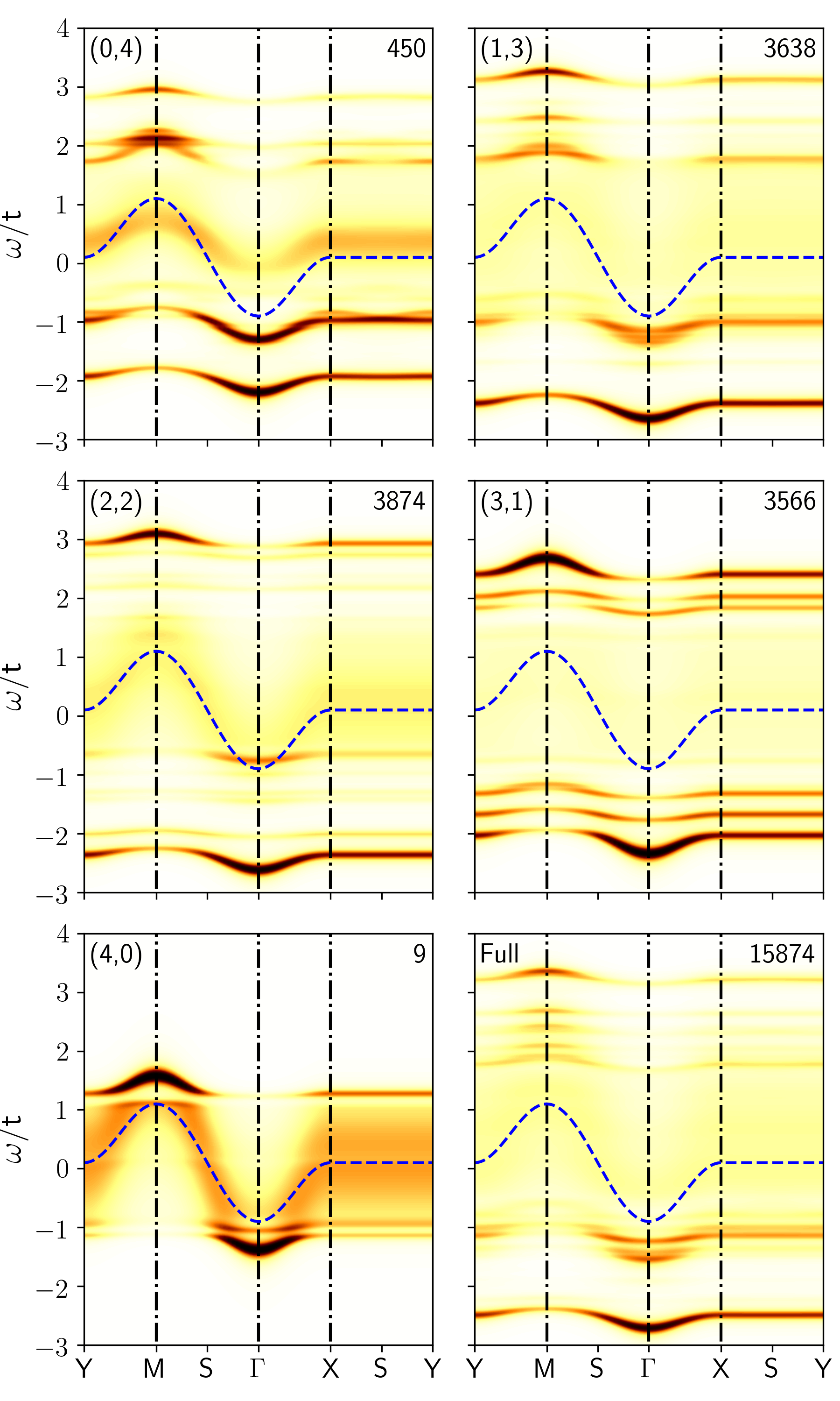
Figure 1: Spectral functions (3) for the case of the Ising model for $J=0.1$ and $S=\tfrac{1}{2}$, presented in nonlinear $\tanh$-scale. The dashed blue line indicates free electron energy $E_{\bm{{k}}}=\epsilon_{\bm{{k}}}+J$. The number in the upper-right corner indicates the number of states generated in the EOM expansion.

The shape and bandwidth of the low-energy QP band, however, is remarkably unaffected by the structure of the cloud, as shown in Fig. 2(a). The magnon-only case has the highest overall energy and the narrowest bandwidth due to being pressed against the continuum. This explains the suppression of the spectral weight at the M point, see Fig. 2(b), and the resulting impression of a $\Gamma$ QP pocket in Fig. 1. The admixture of orbitons stabilizes the polaron, pulling it to lower energies, but without affecting the band shape. As expected, the full solution (the largest variational space) has the lowest energy, below that of the $(1,3)$ and $(2,2)$ subspaces. This shows that there is significant mixing between such configurations in the actual polaron cloud. Thus, this is intrinsically a spin-orbital polaron that cannot be fully described in terms of either spin-only or orbital-only models.

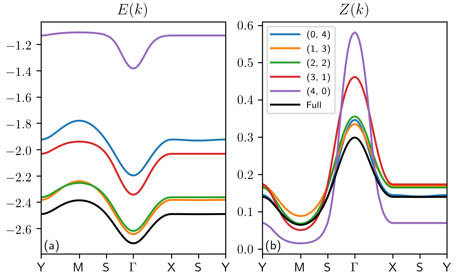
Figure 2: Electron QP energy (left) and spectral weight of the 4th order solutions (right) for $J=0.1$ and $S=\frac{1}{2}$.

A major surprise comes when we consider the evolution of the QP band upon addition of magnons to the cloud. The zero-magnon case implies purely in-plane motion, because magnons are only generated when the electron hops along the $c$ axis. Indeed, here our results agree well with the 2D orbital-polaron of Ref. Bieniasz et al. (2016). Naively, one would expect hopping to another layer to make the polaron much heavier, if not outright incoherent, because the magnon left behind is immobile in the Ising limit. If this magnon is bound into the cloud then the polaron would slow down significantly, whereas if it is unbound, this should result in a finite QP lifetime as the polaron scatters off of it. Indeed, Self-Consistent Born Approximation results support this scenario Bała et al. (2001).

Our results clearly demonstrate that this naive expectation is wrong: the 3D polaron is almost as mobile as its 2D counterpart. To see why, we present results for much smaller variational spaces where the EOMs are simple enough to allow analytical solutions that explain the differences between magnons and orbitons.

Self-energies $\Sigma(\omega)$ for (i) one magnon and (ii) one orbiton allowed into the cloud are derived in the Appendix. They are linked to the propagator through $G(\bm{{k}},\omega)=[\omega+E_{\bm{{k}}}-\Sigma(\bm{{k}},\omega)]^{-1}$, where $E_{\bm{{k}}}=\epsilon_{\bm{{k}}}+J$ is the free electron dispersion. Unlike for bigger variational spaces, in the $(0,1)$ and $(1,0)$ cases the self-energy is momentum-independent making the analysis particularly simple. The right panels of Fig. 3 display the real and imaginary parts of $\Omega=\omega-\Sigma(\omega)$ vs. $\omega$. The vertical dash-dotted lines mark the upper/lower bounds of $E_{\bm{{k}}}$. If $E_{\bm{{k}}}=\omega-\Sigma(\omega)$ for an energy $\omega$ where $\mathrm{Im}\Sigma(\omega)=0$, then a QP with infinite lifetime exists at this $(\bm{{k}},\omega)$ point. If $\mathrm{Im}\Sigma(\omega)\neq 0$, this is an incoherent state in the continuum.

The clear difference is that in the orbiton case (lower panel) there is a QP solution well below the incoherent continuum for all $\bm{{k}}$, whereas in the magnon case, there is a QP solution only for momenta spanning the lower-half of the $E_{\bm{{k}}}$ range. The results are thus qualitatively similar to those presented in Fig. 1: a spin-polaron squeezed just below the continuum as opposed to a well-separated orbiton-polaron band. This is because $\Sigma(\omega)$ is much smaller in the magnon than in the orbiton case [$\mathrm{Re}\Sigma(\omega)$ is the difference between the blue line showing $\omega-\mathrm{Re}\Sigma(\omega)$ and the dashed green line showing $\omega$].

The one-magnon result is $\Sigma_{(1,0)}(\omega)\!=\!2(\frac{t}{2})^{2}G_{00}(\omega\!-\!\frac{3}{2}J)$. This can be understood as follows: the factor of 2 is because the hopping along the $c$ axis can be either to the layer above or below; $t/2$ is the effective hopping between layers, and is squared because the electron must return to the original layer; finally, $G_{nm}(\omega-\frac{3}{2}J)$ is the in-plane propagator for the free electron to move a distance $(n,m)$ away from the site located just above/below the magnon. Thus $G_{00}(\omega)$ controls how likely it is for the two objects to be adjacent. In contrast, for the purely orbiton case, $\Sigma_{(0,1)}(\omega)\,=\,4(\frac{t}{2})^{2}[\,7G_{00}(\omega^{\prime})+2G_{11}(\omega^{\prime})+7G_{20}(\omega^{\prime})\,]/4$, with $\omega^{\prime}=\omega-4J$. There are now four in-plane hopping directions and the hopping integrals are $\frac{t}{2}(1\pm{\sqrt{3}\over 2})$, hence the factors in front of propagators. Finally, there are more ways for the orbiton to be absorbed, which is why several local propagators appear. Below the free particle continuum these propagators decrease exponentially with distance; if we keep only the largest $G_{00}$ contribution, then here $\Sigma_{(0,1)}(\omega)=3.5\Sigma_{(1,0)}(\omega)$. The difference is therefore due to an interplay between dimensionality ($ab$- vs. $c$-axis hopping) and the specific orbital order.

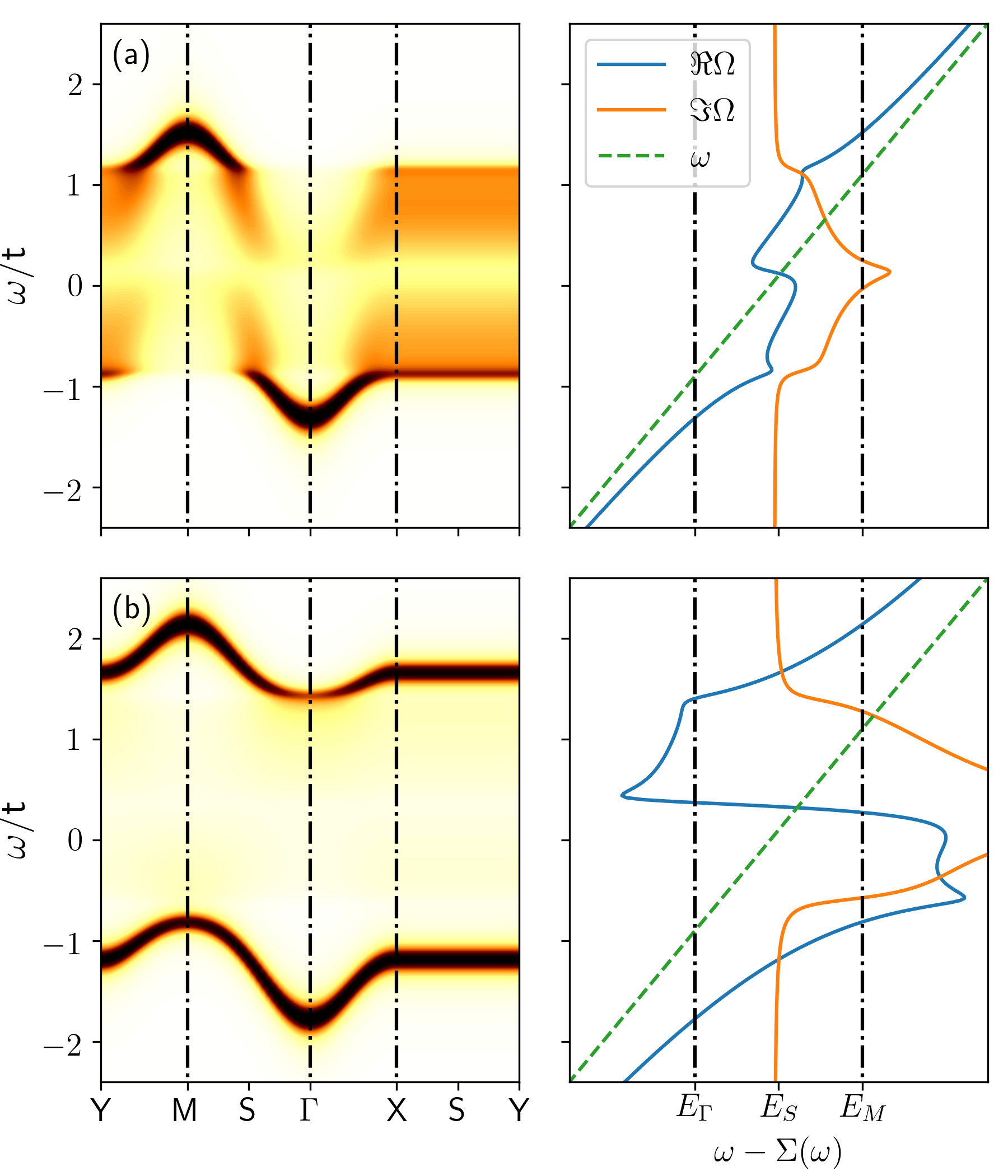
Figure 3: Left— Spectral functions (3) and Right— the real (blue) and imaginary (orange) parts of $\omega-\Sigma(\omega)$ for variational result with a single: (a) magnon and (b) orbiton. Parameters: $J=0.1$, $S=\frac{1}{2}$, and $\eta=0.05$. See text for more details.

This also explains why adding magnons to the polaron cloud will not change its dispersion substantially. Low-order self-energy diagrams involving few bosons are generally non-crossed because magnon and orbiton creation and absorption are accompanied by electron motion in different spatial directions. Thus, to first order the self-energy is the sum of the two separate contributions (higher order crossed magnon-orbiton processes are possible but they involve several bosons and therefore have a low probability and small contributions). Clearly, adding the smaller magnon to the larger orbiton self-energy, has only a limited effect on the QP band, pushing it to lower energies but not changing its shape considerably.

We suggest that the present scenario might work even better for LaMnO₃. The LSDA+$U$ calculations Leonov et al. (2010); Pavarini and Koch (2010) and model calculations Feiner and Oleś (1999); Ishihara et al. (1997); Okamoto et al. (2002) predict $A$-AF/$C$-AO order, as indeed observed Kimura et al. (2003); Zhou and Goodenough (2006); Kovaleva et al. (2010). In this case the configuration of Mn³⁺ ions is $t_{2g}^{3}e_{g}^{1}$ and the leading superexchange terms have the same $T=1/2$ pseudospins but $S=2$ spins Feiner and Oleś (1999) in Eqs. (1) and thus spin and orbital operators are almost disentangled Snamina and Oleś (2016). The bigger spin $S=2$ is exactly counterbalanced by the reduced superexchange $J_{\mathrm{Mn}}=J/4$; hence the absolute energy scale is roughly the same. However, the spin-fermion coupling can only change $S=2$ to $S=1$ which means that the cost of magnons will be roughly 4 times smaller than in KCuF₃, while the orbiton energy is simultaneously amplified by the Jahn-Teller terms Feinberg et al. (1998); Hotta et al. (1999); Snamina and Oleś (2016) making them more classical. This implies that the hole spectral functions for LaMnO₃ are similar to the electron ones for KCuF₃ but the disproportion between magnons and orbitons is even stronger, with less magnon coherence and amplified dominance of orbitons over magnons for the mixed solutions. Indeed, it was found that orbital polarization around a hole can lead to a very narrow QP band and to large incoherent spectral weight Bała et al. (2002), indicating hole confinement in a lightly doped LaMnO₃ insulator.

V Conclusions

We presented variational solutions for the polaron that forms in doped KCuF₃ or LaMnO₃. Comparison of different cloud structures shows that the polaron has intrinsic spin-orbital nature. The presence of magnons, however, is not detrimental to the resulting QP speed and/or lifetime. This is a direct consequence of the spin-orbital ground state that enforces the creation of magnons when the electron (or hole) hops along the $c$ axis Martínez and Horsch (1991). In contrast, the non-conservation of orbital flavor allows for free in-plane electron (hole) propagation and for stronger electron-orbiton interactions promoting robust polarons, both in KCuF₃ and in LaMnO₃.

*

Appendix A Derivation of the one-boson solutions

We use a well-established variational method Berciu (2006); Marchand et al. (2010); Berciu and Fehske (2011); Ebrahimnejad et al. (2016) and allow only for a single excitation by a propagating electron. In general, generating the equations of motion (EOMs) in the variational method proceeds along the same lines regardless of the order of expansion. Therefore, this Appendix will also serve to demonstrate the method itself to the unfamiliar reader. The two solutions we have presented in the main text are the Green’s functions obtained with the generation of:
(a) a single magnon or
(b) a single orbiton.

We start from expanding the resolvent operator according to the Dyson equation:

$$\langle\bm{{k}}\rvert\mathcal{G}(\omega)\lvert\bm{{k}}\rangle=\langle\bm{{k}}\rvert[1+\mathcal{G}(\omega)\mathcal{V}]\\ \times\frac{1}{\sqrt{N}}\sum_{i}e^{i\bm{{k}}\bm{{R}}_{i}}f_{i}^{{\dagger}}\lvert 0\rangle G_{0}(\bm{{k}},\omega-J),$$ (4)

where $G_{0}(\bm{{k}},\omega)=1/(\omega+i\eta-\epsilon_{\bm{{k}}})$ is the free electron propagator. Next, we need to evaluate the result of $\mathcal{V}f_{i}^{{\dagger}}\lvert 0\rangle$, which will generate bosons in the system.

In case (a) the boson stands for a magnon which results from the fermion hopping along direction the $c$ axis according to $\mathcal{V}_{\parallel}^{t}$. This leads to the following EOM for the function $G(\bm{{k}},\omega)$:

$$G(\bm{{k}},\omega)=\left[1-\frac{t}{2}\sum_{\delta\parallel c}F_{1}(\bm{{k}},\omega,\delta)\right]G_{0}(\bm{{k}},\omega-J),$$ (5)

where

$$F_{1}(\bm{{k}},\omega,\delta)=\langle\bm{{k}}\rvert\mathcal{G}(\omega)\frac{1}{\sqrt{N}}\sum_{i}e^{i\bm{{k}}\bm{{R}}_{i}}b_{i}^{{\dagger}}f_{i+\delta}^{{\dagger}}\lvert 0\rangle$$ (6)

is a generalized Green’s function for a single magnon state. This function is unknown and needs to be expanded as before, based on the Dyson equation. However, this time $\mathcal{G}_{0}(\omega)$ acts on a state with a magnon present, which means the electron cannot move far away from its place, otherwise it cannot de-excite the system by removing the magnon. This means that the system is no longer translational invariant and the electron cannot propagate freely to all sites in the system, but has to return back to the vicinity of the magnon; thus $\bm{{k}}$ is no longer a good quantum number. Instead, the electron has to be described in terms of real space Green’s functions

$$G_{mn}(\omega)=\frac{1}{4\pi^{2}}\int\limits_{-\pi}^{\pi}d^{2}kG_{0}(\bm{{k}},\omega)e^{i\bm{{k}}\cdot(m,n,0)},$$ (7)

which describe the propagation of an electron between two in-plane sites, separated by a vector $(m,n)$ lying in the $ab$ plane.

It can be shown that they may be expressed in terms of complex analytical continuation of elliptic integrals of the first and second kind. In the case of a single magnon solution, the electron and the magnon are in two neighboring planes, therefore the free electron propagation will be described by the function $G_{(0,0)}(\omega)$. This leads us to the following expansion:

$$F_{1}(\bm{{k}},\omega,\delta)=-\frac{t}{2}\left[G(\bm{{k}},\omega)+F_{2}(\bm{{k}},\omega,\delta,\delta)\right]G_{00}(\omega-\tfrac{3}{2}J),$$ (8)

where $F_{2}(\bm{{k}},\omega,\delta,\delta)$ is a generalized Green’s function for two magnons in a row. Normally, the expansion would also include functions describing states involving orbitons, but we ignore them in the purely magnonic solution in the lowest order. Moreover, since we are investigating a single magnon solution, we set $F_{2}=0$, thereby closing the EOM system, which now consists of three equations. Solving this system of equations produces the result:

$$G(\bm{{k}},\omega)=\left[\omega+i\eta-\epsilon_{\bm{{k}}}-J-\tfrac{1}{2}t^{2}G_{00}(\omega-\tfrac{3}{2}J)\right]^{-1}.$$ (9)

In case (b) of the one orbiton solution, the first expansion leads to:

$$G(\bm{{k}},\omega)=\left[1-\frac{t}{2}\sum_{\delta\perp c}F_{1}(\bm{{k}},\omega,\delta)\mp\frac{\sqrt{3}t}{4}\sum_{\delta\perp c}\bar{F}_{1}(\bm{{k}},\omega,\delta)\right]\\ \times G_{0}(\bm{{k}},\omega-J).$$ (10)

This time however, the $\delta$ summation goes over the four in-plane directions. $F_{1}$ is defined similarly as before and there is another function:

$$\bar{F}_{1}(\bm{{k}},\omega,\delta)=\langle\bm{{k}}\rvert\mathcal{G}(\omega)\frac{1}{\sqrt{N}}\sum_{i}e^{i(\bm{{k}}+\bm{{Q}})\bm{{R}}_{i}}b_{i}^{{\dagger}}f_{i+\delta}^{{\dagger}}\lvert 0\rangle,$$ (11)

where $\bm{{Q}}=(\pi,\pi,0)$ is the vector characterizing the orbital order the ground state. Its explicit appearance in the equations is due to the non-conservation of the orbital pseudospin. Expansion of the $F_{1}$ functions yields:

$$F_{1}(\bm{{k}},\omega,\delta)=-\frac{t}{4}\sum_{\gamma}\left[2G(\bm{{k}},\omega)\pm\sqrt{3}\bar{G}(\bm{{k}},\omega)\right]\\ \times\tilde{G}_{0}(\bm{{R}}_{i}+\gamma,\bm{{R}}_{i}+\delta,\omega-4J),$$ (12)

$$\bar{F}_{1}(\bm{{k}},\omega,\delta)=-\frac{t}{4}\sum_{\gamma}\left[2\bar{G}(\bm{{k}},\omega)\pm\sqrt{3}G(\bm{{k}},\omega)\right]\\ \times\tilde{G}_{0}(\bm{{R}}_{i}+\gamma,\bm{{R}}_{i}+\delta,\omega-4J),$$ (13)

where we have already neglected the higher order functions. Also, in this analytical solution, the fermion-boson swap term $\propto a_{i}a_{j}^{{\dagger}}f_{i}^{{\dagger}}f_{j}$ of $\mathcal{V}_{\perp}^{t}$ is neglected for simplicity.

Furthermore, this time the fermion and the boson are located in the same plane, so the fermion can end up on any of the sites neighboring the boson, but it is forbidden from entering the boson’s site. Moreover, a careful inspection of the Ising Hamiltonian shows that the cost of a state with the fermion neighboring the boson is lower than that when the fermion is located farther away. The real space Green’s functions have to be corrected for these effects, which is again done using the Dyson equation, with the interaction made to cancel the hopping elements to and from the boson’s site:

$$\mathcal{V}_{i}=\frac{t}{4}\sum_{\epsilon}(f_{i}^{{\dagger}}f_{i+\epsilon}+\mathrm{H.c.})-\tfrac{3}{4}J\sum_{\epsilon}f_{i+\epsilon}^{{\dagger}}f_{i+\epsilon}.$$ (14)

The Dyson expansion of the corrected Green’s functions leads to the equation:

$$\tilde{G}_{0}(\bm{{R}}_{m},\bm{{R}}_{n},\omega)=G_{0}(\bm{{R}}_{m},\bm{{R}}_{n},\omega-\tfrac{9}{2}J)+\\ +\sum_{\epsilon}\tilde{G}_{0}(\bm{{R}}_{m},\bm{{R}}_{i}+\epsilon,\omega)\left[\tfrac{t}{4}G_{0}(\bm{{R}}_{i},\bm{{R}}_{n},\omega-\tfrac{9}{2}J)\right.\\ \left.-\tfrac{3}{4}JG_{0}(\bm{{R}}_{i}+\epsilon,\bm{{R}}_{n},\omega-\tfrac{9}{2}J)\right].$$ (15)

Unlike the regular real space Green’s functions $G_{mn}$ which are defined by the propagation vector $(m,n)$, the corrected functions $\tilde{G}_{0}$, depend on both the starting and final positions explicitly, since the presence of the boson at site $\bm{{R}}_{i}$ breaks the translational symmetry of the system. More details on the practical details of solving the above equation can be found in Bieniasz et al. (2016).

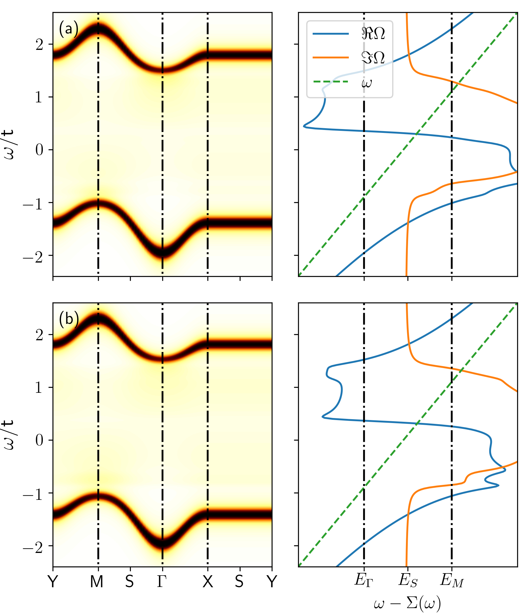
Figure 4: Spectral function (left) and self-energy plots (right) for the full 1st order solutions, without renormalization (a), and with renormalization (b), resulting from the $\mathcal{V}_{\parallel}^{t}$ Hamiltonian. Parameters: $J=0.1$, $S=\frac{1}{2}$.

Finally, the function $\bar{G}(\bm{{k}},\omega)=\langle\bm{{k}}\rvert\mathcal{G}(\omega)\lvert\bm{{k}}+\bm{{Q}}\rangle$ expands into:

$$\bar{G}(\bm{{k}},\omega)=-\frac{t}{4}\sum_{\delta}\left[2\bar{F}_{1}(\bm{{k}},\omega,\delta)\pm\sqrt{3}F_{1}(\bm{{k}},\omega,\delta)\right]\\ \times G_{0}(\bm{{k}}+\bm{{Q}},\omega-J).$$ (16)

In total, this makes ten equations, which can be solved to yield, after some simplification:

$$G(\bm{{k}},\omega)=\left[\omega+i\eta-\epsilon_{\bm{{k}}}-J-\tfrac{1}{2}t^{2}G_{(1,1)}(\omega-4J)\right.\\ \left.-\tfrac{7}{4}t^{2}(G_{(0,0)}(\omega-4J)+G_{(2,0)}(\omega-4J))\right]^{-1}.$$ (17)

If we would now consider the full first order solution, i.e., up to one boson of any kind, we will find that in this case the self-energies are a simple sum of the single flavor solutions, since there are no processes linking the two sectors of the variational space. Furthermore, there will also be a renormalization of the magnonic self-energy resulting from the $a_{i+\delta}^{{\dagger}}b_{i}f_{i}^{{\dagger}}f_{i+\delta}$ process in the $\mathcal{V}_{\parallel}^{t}$ Hamiltonian, which produces a new state, with the fermion and the orbiton located in different planes:

$$\Sigma_{1}(\omega)=\tfrac{1}{2}t^{2}G_{(1,1)}(\omega-4J)\\ +\tfrac{7}{4}t^{2}(G_{(0,0)}(\omega-4J)+G_{(2,0)}(\omega-4J))\\ +\tfrac{1}{2}t^{2}G_{00}(\omega-\tfrac{3}{2}J)/[1-\tfrac{1}{4}t^{2}G_{00}(\omega-4J)].$$ (18)

Figure 4 presents the spectral function and the self-energy plots for these full first order solutions. Clearly, the mixing of magnons and orbitons does not lead to loss of coherence, and this solution is indeed qualitatively very similar to the purely orbitonic one, shown in Fig. 3(b) in the main text. This result supports the explanation given in the main text for the rather small effect of the magnons on the QP dispersion, as being due to the much smaller contribution of magnons to the self-energy because of different dimensionality and the specific ground-state orbital order.

References

- Imada M. and Tokura (1998) A. Imada M., Fujimori and Y. Tokura, Rev. Mod. Phys. 70, 1039 (1998).
- Lee et al. (2006) P. A. Lee, N. Nagaosa, and X.-G. Wen, Rev. Mod. Phys. 78, 17 (2006).
- Martínez and Horsch (1991) G. Martínez and P. Horsch, Phys. Rev. B 44, 317 (1991).
- Tokura and Nagaosa (2000) Y. Tokura and N. Nagaosa, Science 288, 462 (2000).
- Kugel and Khomskii (1982) K. I. Kugel and D. I. Khomskii, Sov. Phys. Usp. 25, 231 (1982).
- Feiner et al. (1997) L. F. Feiner, A. M. Oleś, and J. Zaanen, Phys. Rev. Lett. 78, 2799 (1997).
- Feiner et al. (1998) L. F. Feiner, A. M. Oleś, and J. Zaanen, J. Phys.: Condens. Matter 10, L555 (1998).
- Feiner and Oleś (1999) L. F. Feiner and A. M. Oleś, Phys. Rev. B 59, 3295 (1999).
- Khaliullin and Maekawa (2000) G. Khaliullin and S. Maekawa, Phys. Rev. Lett. 85, 3950 (2000).
- Khaliullin et al. (2001) G. Khaliullin, P. Horsch, and A. M. Oleś, Phys. Rev. Lett. 86, 3879 (2001).
- Horsch et al. (2008) P. Horsch, A. M. Oleś, L. F. Feiner, and G. Khaliullin, Phys. Rev. Lett. 100, 167205 (2008).
- Khaliullin et al. (2004) G. Khaliullin, P. Horsch, and A. M. Oleś, Phys. Rev. B 70, 195103 (2004).
- Oleś et al. (2005) A. M. Oleś, G. Khaliullin, P. Horsch, and L. F. Feiner, Phys. Rev. B 72, 214431 (2005).
- Khaliullin (2005) G. Khaliullin, Prog. Theor. Phys. Suppl. 160, 155 (2005).
- Krüger et al. (2009) F. Krüger, S. Kumar, J. Zaanen, and J. van den Brink, Phys. Rev. B 79, 054504 (2009).
- Wohlfeld et al. (2011) K. Wohlfeld, M. Daghofer, S. Nishimoto, G. Khaliullin, and J. van den Brink, Phys. Rev. Lett. 107, 147201 (2011).
- Wohlfeld et al. (2013) K. Wohlfeld, S. Nishimoto, M. W. Haverkort, and J. van den Brink, Phys. Rev. B 88, 195138 (2013).
- Chen et al. (2015) C.-C. Chen, M. van Veenendaal, T. P. Devereaux, and K. Wohlfeld, Phys. Rev. B 91, 165102 (2015).
- Eremin et al. (2011) M. V. Eremin, J. Deisenhofer, R. M. Eremina, J. Teyssier, D. van der Marel, and A. Loidl, Phys. Rev. B 84, 212407 (2011).
- Corboz et al. (2012) P. Corboz, M. Lajkó, A. M. Läuchli, K. Penc, and F. Mila, Phys. Rev. X 2, 041013 (2012).
- Nasu and Ishihara (2013) J. Nasu and S. Ishihara, Phys. Rev. B 88, 094408 (2013).
- Nasu and Ishihara (2015) J. Nasu and S. Ishihara, Phys. Rev. B 91, 045117 (2015).
- Brzezicki et al. (2015) W. Brzezicki, A. M. Oleś, and M. Cuoco, Phys. Rev. X 5, 011037 (2015).
- Brzezicki et al. (2016) W. Brzezicki, M. Cuoco, and A. M. Oleś, J. Supercond. Nov. Magn. 29, 563 (2016).
- Brzezicki et al. (2017) W. Brzezicki, M. Cuoco, and A. M. Oleś, J. Supercond. Nov. Magn. 30, 129 (2017).
- van den Brink et al. (2000) J. van den Brink, P. Horsch, and A. M. Oleś, Phys. Rev. Lett. 85, 5174 (2000).
- Bała et al. (2001) J. Bała, G. A. Sawatzky, A. M. Oleś, and A. Macridin, Phys. Rev. Lett. 87, 067204 (2001).
- Yin et al. (2001) W.-G. Yin, H.-Q. Lin, and C.-D. Gong, Phys. Rev. Lett. 87, 047204 (2001).
- Ishihara (2005) S. Ishihara, Phys. Rev. Lett. 94, 156408 (2005).
- Daghofer et al. (2008) M. Daghofer, K. Wohlfeld, A. M. Oleś, E. Arrigoni, and P. Horsch, Phys. Rev. Lett. 100, 066403 (2008).
- Wohlfeld et al. (2008) K. Wohlfeld, M. Daghofer, A. M. Oleś, and P. Horsch, Phys. Rev. B 78, 214423 (2008).
- Wohlfeld et al. (2009) K. Wohlfeld, A. M. Oleś, and P. Horsch, Phys. Rev. B 79, 224433 (2009).
- Berciu (2009) M. Berciu, Physics 2, 55 (2009).
- Wróbel and Oleś (2010) P. Wróbel and A. M. Oleś, Phys. Rev. Lett. 104, 206401 (2010).
- van den Brink et al. (1999) J. van den Brink, P. Horsch, F. Mack, and A. M. Oleś, Phys. Rev. B 59, 6795 (1999).
- Feiner and Oleś (2005) L. F. Feiner and A. M. Oleś, Phys. Rev. B 71, 144422 (2005).
- Chao et al. (1977) K. A. Chao, J. Spałek, and A. M. Oleś, J. Phys. C 10, L271 (1977).
- Daghofer et al. (2004) M. Daghofer, A. M. Oleś, and W. von der Linden, Phys. Rev. B 70, 184430 (2004).
- Chernyshev et al. (2000) A. L. Chernyshev, A. H. Castro Neto, and A. R. Bishop, Phys. Rev. Lett. 84, 4922 (2000).
- Fleck et al. (2001) M. Fleck, A. I. Lichtenstein, and A. M. Oleś, Phys. Rev. B 64, 134528 (2001).
- Wróbel et al. (2008) P. Wróbel, W. Suleja, and R. Eder, Phys. Rev. B 78, 064501 (2008).
- Mierzejewski et al. (2011) M. Mierzejewski, L. Vidmar, J. Bonča, and P. Prelovšek, Phys. Rev. Lett. 106, 196401 (2011).
- Oleś et al. (2000) A. M. Oleś, L. F. Feiner, and J. Zaanen, Phys. Rev. B 61, 6257 (2000).
- Lake et al. (2005) B. Lake, D. A. Tennant, C. D. Frost, and S. E. Nagler, Nature Mat. 4, 329 (2005).
- Paolasini et al. (2002) L. Paolasini, R. Caciuffo, A. Sollier, P. Ghigna, and M. Altarelli, Phys. Rev. Lett. 88, 106403 (2002).
- Caciuffo et al. (2002) R. Caciuffo,L. Paolasini, A. Sollier, P. Ghigna, E. Pavarini, J. van den Brink, and M. Altarelli, Phys. Rev. B 65, 174425 (2002).
- Deisenhofer et al. (2008) J. Deisenhofer,I. Leonov, M. V. Eremin, C. Kant, P. Ghigna, F. Mayr, V. V. Iglamov, V. I. Anisimov, and D. van der Marel, Phys. Rev. Lett. 101, 157406 (2008).
- Binggeli and Altarelli (2004) N. Binggeli and M. Altarelli, Phys. Rev. B 70, 085117 (2004).
- Pavarini et al. (2008) E. Pavarini, E. Koch, and A. I. Lichtenstein, Phys. Rev. Lett. 101, 266405 (2008).
- Leonov et al. (2010) I. Leonov, D. Korotin, N. Binggeli, V. I. Anisimov, and D. Vollhardt, Phys. Rev. B 81, 075109 (2010).
- Goodenough (1963) J. B. Goodenough, Magnetism and the Chemical Bond (Wiley, New York, 1963).
- Kanamori (1959) J. Kanamori, J. Phys. Chem. Sol. 10, 87 (1959).
- Note (2) In experimental systems AO order depends on Bała et al. (2001).
- Berciu (2006) M. Berciu, Phys. Rev. Lett. 97, 036402 (2006).
- Marchand et al. (2010) D. J. J. Marchand,G. De Filippis, V. Cataudella, M. Berciu, N. Nagaosa, N. V. Prokof’ev, A. S. Mishchenko, and P. C. E. Stamp, Phys. Rev. Lett. 105, 266605 (2010).
- Berciu and Fehske (2011) M. Berciu and H. Fehske, Phys. Rev. B 84, 165104 (2011).
- Ebrahimnejad et al. (2016) H. Ebrahimnejad, G. A. Sawatzky, and M. Berciu, J. Phys.: Cond. Mat. 28, 105603 (2016).
- Bieniasz et al. (2016) K. Bieniasz, M. Berciu, M. Daghofer, and A. M. Oleś, Phys. Rev. B 94, 085117 (2016).
- Pavarini and Koch (2010) E. Pavarini and E. Koch, Phys. Rev. Lett. 104, 086402 (2010).
- Ishihara et al. (1997) S. Ishihara, J. Inoue, and S. Maekawa, Phys. Rev. B 55, 8280 (1997).
- Okamoto et al. (2002) S. Okamoto, S. Ishihara, and S. Maekawa, Phys. Rev. B 65, 144403 (2002).
- Kimura et al. (2003) T. Kimura, S. Ishihara, H. Shintani, T. Arima, K. T. Takahashi, K. Ishizaka, and Y. Tokura, Phys. Rev. B 68, 060403 (2003).
- Zhou and Goodenough (2006) J.-S. Zhou and J. B. Goodenough, Phys. Rev. Lett. 96, 247202 (2006).
- Kovaleva et al. (2010) N. N. Kovaleva, A. M. Oleś, A. M. Balbashov, A. Maljuk, D. N. Argyriou, G. Khaliullin, and B. Keimer, Phys. Rev. B 81, 235130 (2010).
- Snamina and Oleś (2016) M. Snamina and A. M. Oleś, Phys. Rev. B 94, 214426 (2016).
- Feinberg et al. (1998) D. Feinberg, P. Germain, M. Grilli, and G. Seibold, Phys. Rev. B 57, R5583 (1998).
- Hotta et al. (1999) T. Hotta, S. Yunoki, M. Mayr, and E. Dagotto, Phys. Rev. B 60, R15009 (1999).
- Bała et al. (2002) J. Bała, A. M. Oleś, and P. Horsch, Phys. Rev. B 65, 134420 (2002).