Characterization and control of linear coupling using turn-by-turn beam position monitor data in storage rings
Abstract
We introduce a new application of measuring symplectic generators to characterize and control the linear betatron coupling in storage rings. From synchronized and consecutive BPM (Beam Position Monitor) turn-by-turn (TbT) readings, symplectic Lie generators describing the coupled linear dynamics are extracted. Four plane-crossing terms in the generators directly characterize the coupling between the horizontal and the vertical planes. Coupling control can be accomplished by utilizing the dependency of these plane-crossing terms on skew quadrupoles. The method has been successfully demonstrated to reduce the vertical effective emittance down to the diffraction limit in the newly constructed National Synchrotron Light Source II (NSLS-II) storage ring. This method can be automatized to realize linear coupling feedback control with negligible disturbance on machine operation.
pacs:
41.85.-p, 29.20.dbI Introduction
Linear betatron coupling due to tilting normal quadrupoles, vertical displacement of beam orbit through sextupoles, or existence of skew quadrupoles for vertical dispersion control, can directly degrade machine performance in circular accelerators, such as electron storage rings used as high-brilliance x-ray light sources. Accurate characterization and control of the linear betatron coupling is of primary importance to improve the brilliance for a low-emittance light source. It also provides an important tool for beam volume and intensity related studies.
Thanks to the modern beam diagnostics techniques, turn-by-turn (TbT) beam position monitor (BPM) data are available for most of synchrotron radiation light sources now. From TbT data, a quadratic Lie generator can be extracted by fitting linear one-turn-maps at each BPM location. The coupling between two transverse planes can be directly characterized by four plane-crossing terms in the generators. By using a set of skew quadrupoles at non-dispersive sections, the coupling can be well controlled without blowing up vertical dispersion. This method has been successfully applied to the newly constructed National Synchrotron Light Source II (NSLS-II) storage ring.
There already exist many different analyses of dealing with linear coupling Edwards and Teng (1973); Mais and Ripken (1982); Willeke and Ripken (1989); Sagan et al. (2000); Sagan and Rubin (1999); Lebedev and Bogacz (2010); Guignard (1975); Fischer (2003); Cai (2003); Luo (2004); Aiba et al. (2012); Franchi et al. (2007, 2011); Masaki et al. (2009); Calaga et al. (2005). Some of them are well-known in our community, such as, Teng-Edwards parameterization (symplectic matrix normalization Edwards and Teng (1973)), Mais-Ripken parameterization (generalized Courant-Snyder parameterization with four functions Mais and Ripken (1982); Willeke and Ripken (1989); Lebedev and Bogacz (2010)), and Guignard’s perturbation theory Guignard (1975). In practice, coupling correction is also carried out by minimizing the off-diagonal orbit response matrix Aiba et al. (2012), which is also a fitting module in LOCO Safranek (1997). The purpose of this paper is to emphasize an algorithm using two neighboring BPMs turn-by-turn data to extract the coupling term in their one-turn generators, then to realize coupling control with skew quadrupoles. Benefited from previous analyses, we can demonstrate that direct minimization of coupling terms in the generators is equivalent to these methods. Since TbT data can be accessed within seconds, then skew quadrupole correction scheme can be automatized as a feedback with a negligible interruption on machine routine operation. For ring-based light sources, when insertion devices gaps are being closed or opened, the coupling caused by the imperfection of those devices can be under control.
The paper is organized in the following way: Sect. II introduces coupled 2-dimensional linear Hamiltonian dynamics. Sect. III describes the detailed procedure of extracting one-turn-maps, and then Lie generators from beam TbT data. Sect. IV explains the algorithm of implementing coupling control or correction. In Sect. V, we demonstrate its application on the NSLS-II storage ring. A brief summary is given in Sect. VI.
II Linear coupling
Consider a 2-dimensional (4-dimensinal phase space) coupled linear periodic dynamical system, such as a charged particle traveling in a storage ring. Particle coordinates in the phase space are denoted by , the 4 dimensional vector with the positions and momenta at location . Here means the transpose of vector or matrix . The one-turn-map transforms the vector at turn to at turn
| (1) |
is a matrix observed at the location of and can be written as.
| (2) |
Here and are matrices. In the absence of damping, satisfies the symplecticity condition
| (3) |
in which, is the symplectic matrix
| (4) |
Eq. (3) constrains the number of independent elements of to be 10.
In Lie algebra language, can be interpreted as a quadratic Lie generator Dragt (1982); Chao (2002)
| (5) |
Thus, the transformation of through the matrix is equivalent to a exponential Lie map transformation,
| (6) |
Here, is the component of . There are also 10 independent quadratic terms in , which correspond the 10 independent elements in .
The coefficients of monomial terms in are determined by solving a symmetric, positive definite matrix from
| (7) |
And the Lie generator reads as
| (8) |
Here, is the uncoupled generator. is the linear coupling generator, which includes four plane-crossing terms, and . The coefficients of terms actually characterize the linear coupling between two planes. Our algorithm is to extract the coefficients of from TbT data, then to minimize them with non-dispersive skew quadrupoles directly.
Based on previous analyses accomplished by others, some parameterizations can be derived from the coupled Lie generator . Here we briefly discuss how these parameterizations are related to . In Sect.V, we will compute these parameters using TbT data before and after correction to demonstrate that our algorithm is equivalent to these previous analyses.
First, the fully-coupled matrix and the Lie generator can be converted through Eq.(6) directly. The coupling strength can be observed from two non-zero off-diagonal blocks and . Quantitatively Edwards and Teng normalized to a block-diagonal normal mode format Edwards and Teng (1973). The coupling can be characterized by a symplectic matrix and a phase .
Mais and Ripken Mais and Ripken (1982) proposed another parameterization with four generalized eigenvectors of . In this case two modes and , and four -functions can be derived to describe the frequency and the envelope functions of betatron oscillation. In each plane, the betatron oscillation is composed of two linear independent modes
| (9) |
where , and are the generalized Courant-Snyder betatron envelope functions and phase advances for two modes and . and are constants determined by initial conditions. They will degenerate to the standard Courant-Snyder parameterization when coupling vanishes.
The fully coupled Lie generator can be separated into two parts as Eq. (8), uncoupled part , and coupled part . First, the uncoupled part can parameterized with Courant-Snyder normalization as
| (10) |
Here, is the betatron phase advance per turn, and are the Twiss parameters at , and are the action variables. Then four coupled terms,
| (11) |
can be expressed as a summation of the resonance basis of
| (12) |
Where
| (13) |
are the resonance basis of non-coupled in Eq. (10). and in Eq. (10) and (13) are the action-angle canonical variables. Thus, two pairs of complex conjugates coefficients characterize the coupling
| (14) |
in which is referred as linear sum resonance driving term (RDT), because it can drive a sum resonance when the system tune is close to the resonance line . is defined as difference RDT for the same reason. Ref. Calaga et al. (2005) proves that the RDTs can be merged with Edwards-Teng parameterization Edwards and Teng (1973).
Assuming the system is decoupled at a certain observation point , in the matrix language, two off-diagonal blocks in ; in Lie algebra language, four plane-crossing terms disappear from of Eq. (5); and and in Mais-Ripken’s parameterization also degenerate to zeros, so are RDTs in (14). In other words, the off-diagonal matrices and in , the crossing terms in , two RDTs, and two coupling -functions characterize a common physics quantity - linear coupling observed at the location of this specific position . The goal of linear coupling control is to minimize these non-zero terms.
It is worthwhile to point out that, even though a system is decoupled at one observation point, it is not necessarily decoupled at another one. This is clear since is -dependent. For ring-based light sources, it is crucial to control the coupling at insertion device locations.
III Experimental characterization of linear coupling
In this section, we discuss how to characterize the coupling with BPMs’ TbT readings experimentally, some other techniques can be found in Sagan and Rubin (1999); Huang et al. (2010). In order to obtain synchronized and consecutive TbT data, the beam needs to be excited by pulse magnets, then all BPM readings must be timed with the pulse magnets triggering event within one revolutionary period. From the TbT data array, we first choose two neighboring BPMs, and , with only a few magnets in-between, and assume the linear transforming matrix between these two BPMs is known. By ignoring damping and de-coherence, the two BPMs’ readings (after subtracting the closed orbit) at the turn are related by
| (15) |
With Eq. (15), at both BPMs are determined. Therefore we obtain beam coordinates in phase space at the locations of the two BPMs for multiple turns. Then the one-turn-map at the location of the BPM is the least-squares solution of the linear equations for multiple turns.
| (16) |
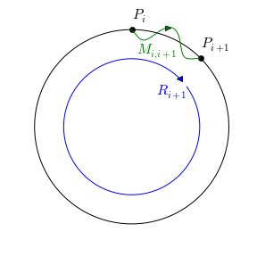
In principle, two consecutive turns data can uniquely define a one-turn map. But due to various errors from BPMs readings, magnet power suppliers jittering, and etc., we have to fit multiple consecutive turns data with the least square method to filter those random errors out. Usually more than 500 turns data are used to solve Eq. (16).
As mentioned before, the couplings seen at different BPMs locations could be different. For a ring-based light source unless for special purpose, e.g. increasing beam volume for longer Touschek life time, it is preferable to have no coupling all over the storage ring, especially at the source points where insertion devices are located. Thus we need to fit out the one-turn-maps at multiple BPM pairs by applying Eq. (15) and (16) repeatedly.
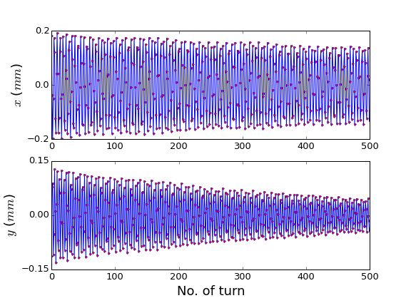
There existes another method to extract the N-turn map to avoid computing in hadron rings Fischer (2003). In the NSLS-II storage ring, a strong amplitude variation due to radiation damping, or decoherence is visible (see Fig. 2) from TbT data. In order to mitigate this effect, we choose two neighboring BPMs to reconstruct momenta , then two consecutive turns data to extract one-turn maps.
Once is obtained, the coefficients of coupling terms , and then RDTs can be calculated with Eqs. (7), (8) and (12) respectively. The two coupling -functions can be calculated with the approach explained in Willeke and Ripken (1989).
One thing needs to be emphasized here is, the direct measured with Eq. (16) is not always exactly symplectic due to various measurement errors. A symplectic matrix can be obtained in the following way. First, can be approximated to a Lie generator using Eq. (7). Then we can act on each canonical variable to get one row of a symplectic matrix as explained in ref. Chao (2002),
| (17) |
Here, only the first row is listed, other three rows can be obtained in the same way. An alternative way of symplectifying is given in ref. Fischer (2003).
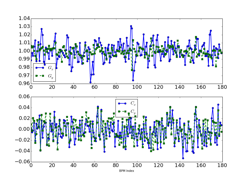
Now we discuss the control of various measurement errors. First, BPM’s imperfections can affect the calculation of and therefore . In order to mitigate these affects, for each BPM, four parameters fitted by the LOCO Safranek (1997, 2007); Yang et al. (2007); Yang (2015) method give the full linear transformation between the raw TbT readings and the realistic beam trajectory :
| (18) |
where, are the gain calibrations, and are the coupling calibrations due to the roll and the associated construction errors. The four parameters vary for each BPM, as shown in Fig. 3. Calibrated data are obtained by implementing the inverse transformation of Eq. (18) on raw data.
BPM resolution is measured as at 10mA stored beam current Cheng (2015). During the coupling characterization, we usually excite beam with an amplitude less than . This resolution can satisfy the requirement of precise characterization of linear coupling.
A systematic error comes from the assumption that the transforming matrix between two BPMs is known in Eq. (15). In order to minimize the effect caused by unknown magnets errors, we intentionally choose two BPMs separated by as few as possible magnets. In the NSLS-II storage ring, only those BPM pairs separated by a long drift () and two sextupoles are used. The closed orbit has been aligned to the center of relevant quadrupoles Portmann et al. (1995) and the closed orbit displacements at the locations of sextupoles are negligible, thus is simplified as a coordinate transformation through a drift. The presence of sextupoles intrinsically affects and as a systematic error. A detailed simulation was set up to study this effect. A set of simulated TbT data was obtained by tracking a particle with a similar transverse amplitude () as we used in the experiment. Then we use momenta in the simulated data to compute the one-turn map directly, and compare it against the map from the momenta reconstructed by the coordinates with the approximated linear transfer map. Two obtained maps are shown as,
| (19) |
and
| (20) |
Consider betatron oscillation amplitude is around , then the difference of TbT readings between these two maps is below . The NSLS-II BPM resolution is around . Therefore, in this particular case, the sextuple effect on TbT data is too weak to be measured experimentally.
In electron storage rings, a systematic error is due to radiation and collective damping. Radiation damping is negligible because we fit the data between two consecutive turns. Collective damping can be mitigated by filling the ring with a low charge per bunch, while BPMs still have reliable readings.
Another error is the decoherence effects caused by non-zero chromaticity and nonlinearity Meller et al. (1987). They can be effectively suppressed by adjusting chromaticities close to zeros, and using low beam excitations separately.
As usual, multiple TbT data collection are repeated for each scenario to suppress any random uncertainty and also are used to estimate measurement error fluctuation. The achieved fluctuations of for multiple measurements are around 5% (see Fig.5).
IV Correction algorithm
Based on the designed lattice model, four plane-crossing terms’ dependence on non-dispersive skew quadrupoles are calculated with
| (21) |
where are the coefficients of Eq. (11) observed at the location of BPMs, is the skew quadrupole normalized focusing strength, is the BPM’s dependence on the skew quadrupole. Once these four coefficients in Eq. (11) at each observation location are measured, the needed skew quadrupole corrections to minimize them are obtained by iteratively solving the following linear equations
| (22) |
Since there are four goal functions per observation location, we vertically stack their response matrices with different weights to minimize them simultaneously.
V Experiment on NSLS-II storage ring
In order to control the vertical beam size, inside each cell of the NSLS-II storage ring, a skew quadrupole is incorporated into the lattice. In the odd numbered cells, it is located in the dispersive region, which can be used for vertical dispersion compensation. And in the even numbered cells, it is located in non-dispersive regions, which can be used for linear coupling correction. With this configuration, we can correct the vertical dispersion first, and then the linear coupling. Actually we can combine these two corrections with a weighted and combined response matrix to correct them simultaneously as suggested in Ref. Franchi et al. (2011). It will become necessary if a different lattice configuration with non-zero dispersion all around the ring.
In this paper, we only focus on the coupling correction. A total of 60 BPMs located in 30 straight sections are used to characterize the coupling. Therefore, each individual response matrix is , as illustrated in Fig. 4. The dimension of stacked response matrix is .
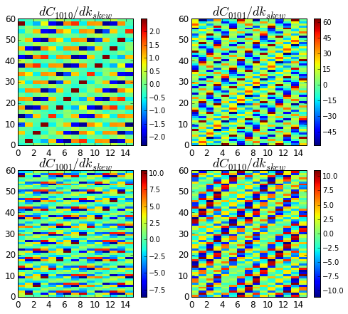
Eq. (22) is solved with SVD algorithm. At each iteration, we only keep those singular values greater than 50% of the largest one in order to minimize corrector strengths.
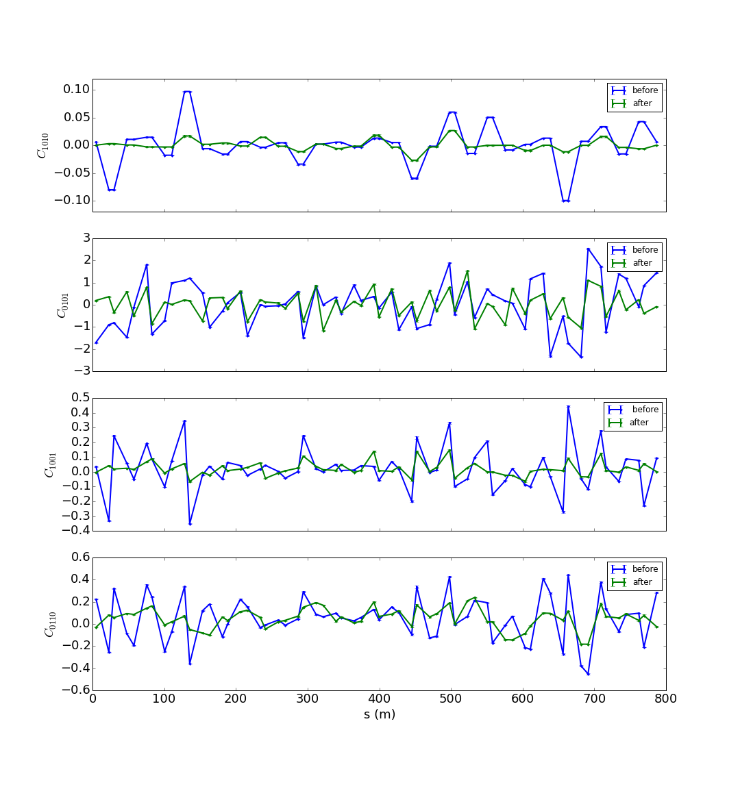
Fig. 5 shows the comparison of four coupling coefficients , , and before and after applying correction. Among them, the suppression on and are obvious at most BPMs.
As explained in Sect. II, several other parameterizations are used to characterize the coupling. Next we calculate and compare their parameters before and after applying correction. It will confirm that, the minimization of the crossing terms in the Lie generator is equivalent to other approaches.
V.1 Linear one-turn-map
The measured one-turn-map seen by one of BPMs before applying the correction reads as
| (23) |
And after three iterative corrections, it becomes
| (24) |
The off-diagonal elements after correction in Eq. (24) are found to be significantly smaller than before correction in Eq. (23). It means that the coupling matrix and in Edwards-Teng parameterization has been reduced successfully.
V.2 Coupling -functions
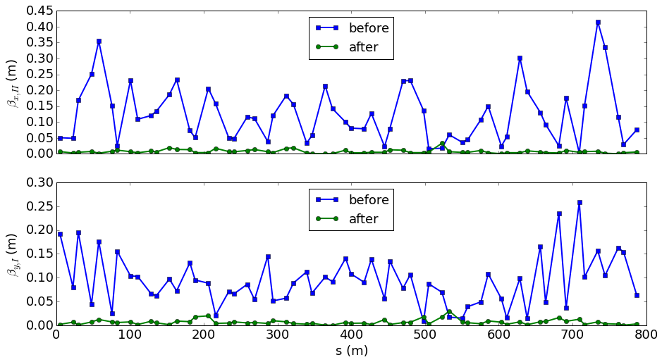
In Mais-Ripken’s parameterization, besides two dominant and , another two small envelope functions and actually represent the coupling motion between two planes. They were calculated from the measured . The comparison is illustrated in Fig. 6. Both the maximum and average values of the two coupling -functions are suppressed significantly after three iterations.
V.3 Resonance driving terms
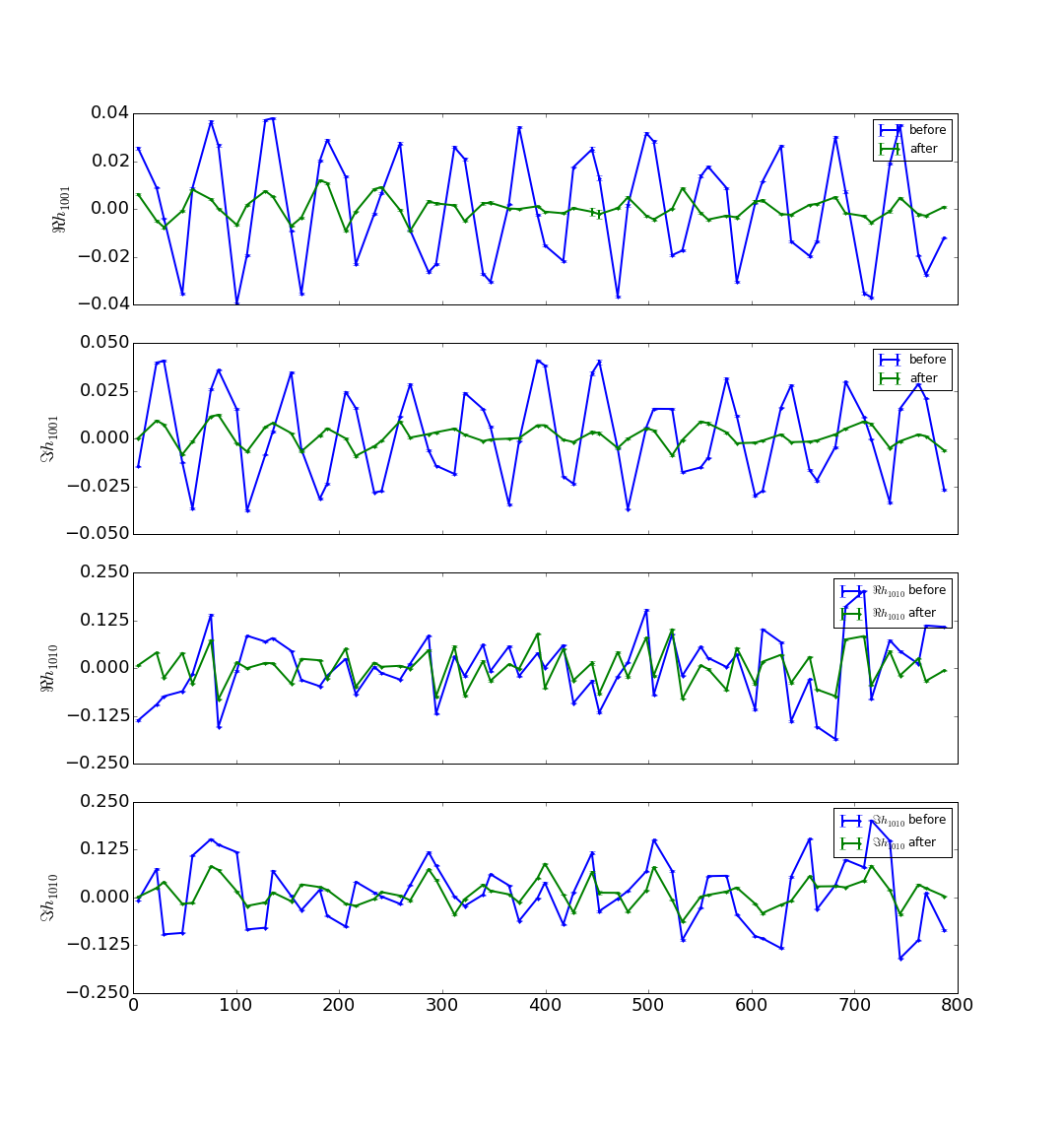
Since the tune of NSLS-II ring tune is close to the difference resonance line , the suppression on RDT are relatively dramatic. Comparison of its real and imagery parts before and after corrections are illustrated as the and plot in Fig. 7 respectively. In the meantime, the suppression on the sum RDT is also visible as shown in the and plots of Fig. 7. It is also possible to correct the sum and difference together using a weighted response matrix of RDTs versus skew quadrupoles Franchi et al. (2011).
V.4 Spectra of Betatron oscillation
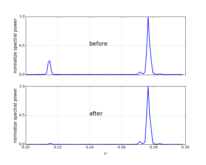
The vertical spectra of the TbT data before and after coupling correction are illustrated in Fig. 8. Before correction, a horizontal betatron mode frequency peak is clearly visible in the vertical spectrum. After applying correction on skew quadrupoles, it has been effectively suppressed.
V.5 Beam transverse profile
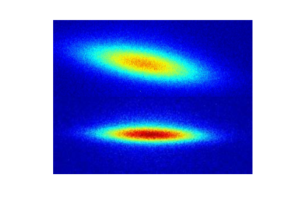
Another direct observation of the linear coupling is beam transverse profile - its tilt angle and vertical size. A x-ray diagnostic beam line configured with a pinhole camera provides the real time beam profiles and its 2D Gaussian fitting dimensions. The CCD camera pixel dimension with respect to beam size image has been well calibrated as by displacing beam at different orbits. Before the coupling correction, beam transverse profile has a tilted angle with the 32 vertical beam emittance. After 3 times iterations, Both the tilt angle and vertical beam size become much smaller than before correction. The profile comparison before and after correction observed by the pinhole camera is shown in Fig. 9.
In the meantime, the phenomenon of beam vertical size reduction was observed at another source point, the Hard X-ray Nano-probe beam line in-vacuum undulator Chubar and Chu (2015). As we mentioned before, our strategy is to minimize the coupling at multiple observation points, especially the locations where insertion devices are located.
V.6 Beam lifetime
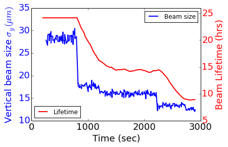
The Touschek lifetime depends on the vertical beam size linearly. The existence of both vertical dispersion and linear coupling can blow up beam size vertically. Therefore, as the corrections were implemented, the beam lifetime was observed to be linearly scaled with the vertical beam size as illustrated in Fig. 10.
VI Summary
From beam turn-by-turn BPM readings, four plane-crossing terms in Lie generators are extracted to characterize linear coupling directly. And coupling control can be realized by utilizing their dependence on the non-dispersive skew quadrupoles. In the meantime, several other parameters, such as, Edwards-Teng symplectic matrix normalization, resonance-driving terms, and Mais-Ripken -functions can be derived from the Lie generators. The application of this approach on the NSLS-II ring successfully control the coupling and reduce the vertical emittance below the diffraction limit. The effectiveness of our coupling correction method has been verified by using another method - independent component analysis (ICA), and reported in Huang and Yang (2015).
Some existing tools, such as LOCO Safranek (1997, 2007) can realize linear coupling correction as a small part of the overall framework. But to measure an orbit response matrix, and then to fit it to a lattice model take some time, which usually needs a dedicated beam study time. A major benefit of using TbT data to characterize and control linear coupling is that it can be automatized as a feedback process during routine operation, because it can accomplish data access and correction within several seconds.
Acknowledgements.
Work was supported by the U.S. Department of Energy, Office of Science, Office of Basic Energy Sciences, under Contract No. DE-AC02-98CH10886.References
- Edwards and Teng (1973) D. Edwards and L. Teng, IEEE Trans.Nucl.Sci. 20, 885 (1973).
- Mais and Ripken (1982) H. Mais and G. Ripken, DESY M-82/05 (1982).
- Willeke and Ripken (1989) F. Willeke and G. Ripken, AIP Conf.Proc. 184, 758 (1989).
- Sagan et al. (2000) D. Sagan, R. Meller, R. Littauer, and D. Rubin, Phys. Rev. ST Accel. Beams 3, 092801 (2000).
- Sagan and Rubin (1999) D. Sagan and D. Rubin, Phys.Rev.ST Accel.Beams 2, 074001 (1999).
- Lebedev and Bogacz (2010) V. Lebedev and S. Bogacz, JINST 5, P10010 (2010), arXiv:1207.5526 [physics.acc-ph] .
- Guignard (1975) G. Guignard, CERN ISR-MA/75-23 (1975).
- Fischer (2003) W. Fischer, Phys. Rev. ST Accel. Beams 6, 062801 (2003).
- Cai (2003) Y. Cai, Phys.Rev. E68, 036501 (2003).
- Luo (2004) Y. Luo, Phys.Rev.ST Accel.Beams 7, 124001 (2004).
- Aiba et al. (2012) M. Aiba, M. Böge, N. Milas, and A. Streun, Nucl.Instrum.Meth. A694, 133–139 (2012).
- Franchi et al. (2007) A. Franchi, E. Métral, and R. Tomás, Phys. Rev. ST Accel. Beams 10, 064003 (2007).
- Franchi et al. (2011) A. Franchi, L. Farvacque, J. Chavanne, F. Ewald, B. Nash, K. Scheidt, and R. Tomás, Phys. Rev. ST Accel. Beams 14, 034002 (2011).
- Masaki et al. (2009) M. Masaki, M. Takao, K. Soutome, and S. Takano, Phys. Rev. ST Accel. Beams 12, 024002 (2009).
- Calaga et al. (2005) R. Calaga, R. Tomas, and A. Franchi, Phys.Rev.ST Accel.Beams 8, 034001 (2005).
- Safranek (1997) J. Safranek, Nucl.Instrum.Meth. A388, 27 (1997).
- Dragt (1982) A. Dragt, AIP Conf.Proc. 87, 147 (1982).
- Chao (2002) A. Chao, SLAC-PUB-9574 (2002).
- Huang et al. (2010) X. Huang, J. Sebek, and D. Martin, Phys.Rev.ST Accel.Beams 13, 114002 (2010).
- Safranek (2007) J. Safranek, ICFA Beam Dyn.Newslett. 44, 43 (2007).
- Yang et al. (2007) L. Yang, S. Lee, X. Huang, and B. Podobedov, Conf.Proc. C070625, 804 (2007).
- Yang (2015) X. Yang, private communication (2015).
- Cheng (2015) W. Cheng, private communication (2015).
- Portmann et al. (1995) G. Portmann, D. Robin, and L. Schachinger, PAC’1995 Proceedings 4, 2693 (1995).
- Meller et al. (1987) R. Meller, A. Chao, J. Peterson, S. G. Peggs, and M. Furman, SSC-N-360 (1987).
- Chubar and Chu (2015) O. Chubar and Y. Chu, private communication (2015).
- Huang and Yang (2015) X. Huang and X. Yang, IPAC’15 Proceedings (2015).