Nonlinear dynamics and chaos Time series analysis Fluctuation phenomena
Symbolic dynamics techniques for complex systems: Application to share price dynamics
Abstract
The symbolic dynamics technique is well-known for low-dimensional dynamical systems and chaotic maps, and lies at the roots of the thermodynamic formalism of dynamical systems. Here we show that this technique can also be successfully applied to time series generated by complex systems of much higher dimensionality. Our main example is the investigation of share price returns in a coarse-grained way. A nontrivial spectrum of Rényi entropies is found. We study how the spectrum depends on the time scale of returns, the sector of stocks considered, as well as the number of symbols used for the symbolic description. Overall our analysis confirms that in the symbol space transition probabilities of observed share price returns depend on the entire history of previous symbols, thus emphasizing the need for a modelling based on non-Markovian stochastic processes. Our method allows for quantitative comparisons of entirely different complex systems, for example the statistics of symbol sequences generated by share price returns using 4 symbols can be compared with that of genomic sequences.
pacs:
05.45.-apacs:
05.45.Tppacs:
05.40.-a1 Introduction
The symbolic dynamics technique is a powerful method to describe trajectories of a dynamical system in a coarse-grained way [1, 2, 3, 4, 5, 6, 7, 8, 9, 10]. It has been applied to many low-dimensional maps exhibiting chaotic or critical behavior. Nontrivial correlations in the dynamical system manifest themselves in a nontrivial spectrum of Rényi entropies [11, 12, 13, 1, 4, 5] and other observables associated with the set of allowed symbol sequences and their corresponding probabilities. This technique, which was very popular in the 80s and 90s when a lot of research on 1-dimensional maps was done [2, 3, 4, 5, 10], has been revived in more recent work and applied in a more general context [14, 15, 16, 17].
Our main aim in this paper is to illustrate that the symbolic dynamics technique borrowed from dynamical systems theory can be successfully applied to time series generated by general complex systems in higher dimensions, far beyond the original 1-dimensional chaotic map approach. Our main example in the following will be share price dynamics, which is of course ultimately produced by a complex market and trader dynamics in a high-dimensional phase space [18]. It is well-known that financial time series exhibit multifractal features [19, 20, 21, 22], but here we present a somewhat different approach to this problem based on the symbolic dynamics technique. We will investigate the correlations and complex behavior associated with discrete symbol sequences generated from observed share price returns on various time scales. We will quantify this by the calculation of the corresponding Rényi entropies [1, 11, 12, 13] for symbol sequences based on historical data sets of share price returns for various sectors, both on long (daily) time scales and on short time scales (minutes). It turns out that the stochastic process of symbol sequences observed for real share price data exhibit non-Markovian character. To characterize differences between various companies (or communities in a complex system context), we will introduce a Rényi difference matrix which compares Rényi entropies of different subsystems. The method developed allows for quantitative comparisons of different complex subsystems, or even different scientific problems due to the encoding in the symbolic dynamics space. For example, it is possible to quantitatively compare the statistical properties of genomic sequences [23, 24, 25] with those generated by coarse-grained share price movements, although both problems come from completely different areas of science.
2 Symbolic dynamics for share prices
Let us apply the symbolic dynamics technique, well known from dynamical systems theory, to a coarse grained description of a given time series. This time series is assumed to be generated by a suitable observable of a dynamically evolving complex system. Rather than being very theoretical, we choose a concrete example: Share price evolution, as created by complex market structures and trader speculations. Often, one is interested only in a very basic question related to a given complex system. For the example of share prices, this question is quite straightforward: Basically one is interested in whether the share price of a particular company will go up or down, and this problem of course also depends on the time scale considered. To generate symbol sequences associated with a question of this type we first need to choose a suitable partition of the phase space (a generating partition in the case of low-dimensional maps).
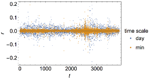
The easiest and most straightforward way for share prices is to consider just two symbols, i.e. to consider the possible values of logarithmic share price returns in two disjoint subsets and , corresponding to negative and positive changes of the share price on a discrete time scale labelled as . This is kind of a reduced phase space description for the question asked here. Note that and are chosen as open intervals. The point 0 (corresponding to no change) has measure 0, it does not influence the analysis. Of course, for other complex systems/time series one can define the subsets generating the symbol sequences differently, that depends on the problem and the question asked about the complex system. In general, much more complicated generating partitions arise in this way [9, 16].
Let’s now look at an example data set of daily stock prices of the company Alcoa Inc. that covers the period January 1998 to May 2013 (Fig. 1). If the log return is an element of , which is equivalent to , then we denote such a price decreasing event by the symbol . Otherwise a price in stands for and is denoted by which means a price increasing. By this method we can attribute to the time series of share prices a symbol sequence where . We now consider subsequences of symbols of length , where is small as compared to the total number of data available. As we only have data for a limited set of data points, we divide up the whole data sequence into segments of equal length . Because each symbol has only two choices which are either or , for any given we get up to allowed subsequences. Since the partition of the phase space is rather simple and our dataset is big enough to satisfy , there will be many occurences that correspond to the same symbolic pattern. Hence we can easily acquire the probabilities of each allowed symbol sequences by determining the frequencies of how often the symbol sequence occurs in the given data set. The probability of a given symbol sequence of length is then denoted as , where labels all possible sequences .
Now by encoding each allowed symbol sequence of length into a real number on the unit interval using the binary expansion with and and , we can produce a plot to visualise our probabilities. This means any given sequence of symbols can be represented by a sequence of bits, in particularly we assign
| (1) |
where . One can implement this by defining a coordinate assigned to a given symbol sequence as
| (2) |
Note that . In this way we allocate to each symbol sequence a real number on the unit interval so that we can easily visualize our results on the frequency of a given symbol sequence. This is shown in Fig.2.
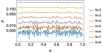
Note that numerically we restrict ourselves to because of the fact that we only have a limited amount of data points. Larger would induce large stochastic errors due to the fact that the statistics is not high enough to estimate the frequency of a given symbol sequence in a reliable way.
Also note that while for the simple example considered here all symbol sequences are possible, for more general complex systems (and more complicated questions asked that are then encoded into the symbols, such as the problems in [14, 15, 16, 17]) there will be a set of allowed and forbidden sequences in the symbol space. In this case the distribution in Fig. 2 will have gaps and generally there will be a multifractal structure. Still everything that we define in this paper can still be done in an analogous way.
3 Information contents of the symbolic sequences
Given experimentally determined probability distributions with possible selfsimilar features such as in Fig. 2, it is meaningful to find a proper way to measure multifractal features. For this purpose we use the well-known concept of Rényi information [1, 11, 12, 13] defined as
| (3) |
Here is a real number and is the number of allowed symbol sequences for a given (an allowed symbol sequence is one satisfying ). The index labels the various sequence probabilities. The Rényi information measure can be regarded as a generalisation of the Shannon information, as for we have
| (4) |
where denotes the Shannon information.
An important special case in Eq.3 is the choice ,
| (5) |
which means decreases in a logarithmical way with the number of allowed symbol sequences. Note that when we have a limited length of symbol sequences, Eq.3 yields a finite value as is finite.
Recall that for a given any symbol sequence is mapped onto a point of , with equal distance between neighboring points. We call the distance of two neighboring coordinates at a given level in Fig. 2 box size and denote it by . In our case the box size is determined by as . That means is getting smaller as grows and when , is approaching 0, in which case the Rényi information defined by Eq.3 diverges. It is then useful to define the Rényi dimension which is a useful quantity as it stays finite in the limit :
| (6) |
An example of (finite box-size) Rényi dimensions evaluated for the data given in Fig. 2 is shown in Fig. 3.
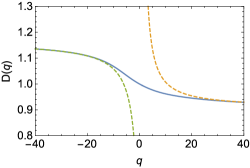
Of course the size of any data set is limited, in our case the smallest that can be achieved with reliable non-fluctuating results is . Given the finiteness of the data set it is useful to check some rigorous upper and lower bounds and monotonicity properties of the Renyi dimensions, valid for arbitrary probability measures. The Rényi dimensions are monotonically decreasing and their values must be positive for all . Also, if all symbol sequences are allowed then we must get the value 1 when . This is because
| (7) |
In addition, as shown in [12] there is a restriction of possible values of Rényi dimensions as a general upper and lower bound dimensions can be proved:
| (8) |
If we substitute and for in Eq.8, we obtain the upper bound
| (9) |
and a lower bound is given by
| (10) |
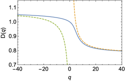
We have checked these bounds for our data set with , the result is also shown in Fig. 3. Clearly the inequalities (9) and (10) are satisfied by our experimental data.
From the Rényi dimensions one can proceed to the singularity spectrum of crowding indices by a Legendre transformation in the thermodynamic formalism. However, as the information contained in spectra is the same as the one in the generalized dimensions , we will not further proceed along these lines here, but refer the reader to suitable literature introducing to this topic [26, 1].
4 Rényi entropies
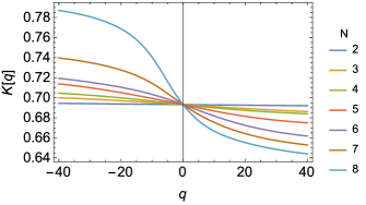
Unlike the Rényi dimension, which generally is a property of a given multifractal probability measure and which does not a priori contain any dynamical information, the Rényi entropy measures the production (or loss) of information encoded in the symbol sequences. This is the quantity of direct interest for share price evolution. The Rényi entropy is defined in the limit and given by
| (11) |
Of course, by projecting symbol sequences onto points on the real line (as done in Fig. 2), both approaches can be made formally equivalent, but the dynamical information is then just encoded in a suitable multifractal measure.
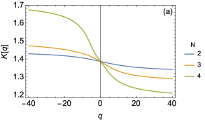
Fig. 4 shows finite- versions of Rényi entropies for share price returns where grows from 2 to 8. The Renyi entropies have of course the same dependence on as the Renyi dimensions of the corresponding multifractal measure that encodes the symbol sequence probabilities on the unit interval.
For we get
| (12) |
which is the topological entropy. Moreover for , using Eq. 4,
| (13) |
we get the Kolmogorov-Sinai entropy asssociated with the symbol sequences of share price changes. Again one can proceed from the function to an equivalent spectrum of dynamical indices by Legendre transformation (see, e.g. [1]).
5 Small time scales
We have quantified the joint probabilities of the daily share price movements by the corresponding Rényi entropies. We are now interested in how these observables depend on the time scale of the symbolic dynamics. Instead of using the daily share prices, the now analysed data set consists of share prices recorded each minute for the same period from 1998 to 2013; this covers about 1.5 million data points. We repeat the same analysis as before and consider symbol sequences up to length 8. By using the same partition method as in the previous section we obtain the multifractal probability distributions of symbol sequences as shown in Fig. 5.
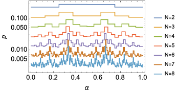
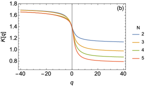
Compared with Fig. 2, the probability distributions on a small time scale are significantly different from those on the daily time scale. Note that there are some local maxima which are reproduced in a self-similar way. While these densities are non-smooth, the advantage of proceeding to the Renyi dimensions (or entropies) is that in this way a smooth dependence on the scanning paramter is produced. This is shown in Fig. 6 and 7.
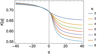
We see, similar to the daily time scale, that both the Rényi entropies and the Rényi dimensions are monotonically decreasing with respect to the paramter , with larger generating a more pronounced -dependence for positive , whereas there is hardly any -dependence for . Fig. 7 also shows the upper and lower bound.
An important property that we have checked for our data sets is the fact that quite generally the conditional probabilities
| (14) |
depend on the entire history , i.e. a Markovian model cannot capture the complex features in the symbol space. For example, given a long alternating sequence it is statistically slightly more likely to observe the next symbol as .
6 4-symbol partitions
So far we used the simplest method to study the symbolic dynamics of the share price movements, just considering whether a share price goes up or down. We may, however, also ask a more detailed question, such as whether the share price goes up slightly or strongly. To detect further details, we may generate a refined version of the phase space partition where previously and . Assume there exists a real number where the log returns have equal 1-point probabilities to fall into each element of a partition given by
| (15) |
In other words, this partition is chosen in such a way that the 1-point probabilities of the log returns lying in each set are identical to . For Alcoa Inc. share prices on daily and minutely time scales, we find is equal to 0.014 and 0.00088, respectively. Instead of denoting the time evolution by and , we re-define our symbol sequence by
| (16) |
where corresponds to a log return in . For a given length , the number of allowed sequences is . We may also upgrade the previous approach to a 4-level symbolic sequence given by
| (17) |
A symbol sequence of length can be encoded as a coordinate on the unit interval based on the representation
| (18) |
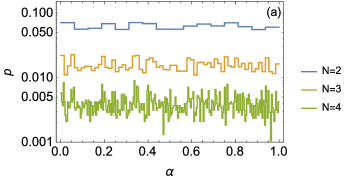
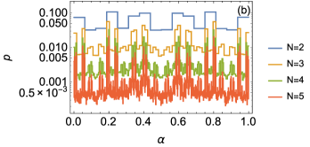
The plot of joint probabilities in the case of an alphabet of 4 symbols is shown in Fig. 8, the corresponding finite- Rényi entropies are shown in Fig. 9.
7 Different companies
So far we only looked at a particular example of a stock, Alcoa shares. The really interesting work on complex system analysis starts when one compares Rényi entropies of different companies, or even Rényi entropies of entirely different complex systems described by the same alphabet of symbols. Ultimately we really want to learn something about the complex market structure and dynamics represented by different companies, sectors, or communities for general complex systems. Still one can let each community generate a suitable time series for a suitable observable and then analyse this time series with the symbolic dynamics technique described so far. We are then interested in differences or similarities of the obtained Renyi entropies.
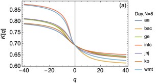

To illustrate this we looked at symbol sequences as generated by share prices of 7 different companies, Alcoa (aa), Bank of America (bac), General Electric (ge), Intel (intc), Johnson & Johnson (jnj), Coca Cola (ko), WalMart (wmt), representing the sectors basic materials, financial, industrial goods, technology, healthcare, consumer goods, services. The results are shown in Fig.10. It can be observed that bac appears to have the lowest Rényi entropy in the region as compared to other stocks, overall the -dependence for financial stocks is most pronounced. This could have to do with the fact that financial stocks have relatively strong fluctuations and exhibit nontrivial correlations, described by a non-trivial spectrum of Rényi entropies. In any case, different companies are characterized by a different spectrum of Rényi entropies both on a daily (Fig. 10a) and minute (Fig. 10b) time scale. The smooth dependence on the parameter can be used for an effective thermodynamic description of the complex behavior involved, with different emphasis given to low and high proababilities depending on the value of the scanning parameter .
8 Quantifying similarities in the symbol sequence statistics
We may now wish to compare in a quantitative way how much the Rényi entropies of different companies (or communities in the general complex system context) differ. For this purpose we define a Rényi difference matrix as follows:
| (19) |
Clearly, if two companies and have the same statistics of symbol sequences, described by the same functional dependence , then the Rényi difference matrix element is . Otherwise, the entry integrates up differences in the Rényi entropy spectra, and averages them over , weighted with the parameter .
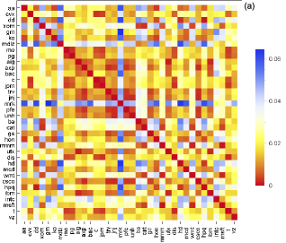
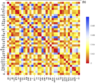
Fig 11 shows a colour encoding of such a Rényi difference matrix. For 36 different companies we evaluated , choosing and . The Rényi difference matrix allows one to single out major differences and similarities in the symbol sequence statistics of different companies/communities in a quantitative way. In our case, for example, the healthcare company Merck (mrk) is identified as having an unusual Rényi entropy spectrum on a daily scale, different from that of most other companies, visible here as a pronounced vertical and horizontal blue line in the pattern generated. On the other hand, on the small time scale of minutes this company is much more similar to the others.
An interesting final remark is at order. Once a suitable question has been asked about a complex system, and a symbolic dynamics constructed, we can then compare different complex systems, or subsystems thereof, whatever their origin, as all relevant information is encoded in the symbol sequence statistics. To give an example, in [24, 25] the complexity of DNA sequences of the human genome was investigated, by calculating the Renyi entropies associated with the sequence statistics of the 4 bases A,T,G,C. Once this function is obtained, it can then be compared using the above Rényi difference matrix with other genomes, in just the same way as we compared the differences between different companies in Fig. 11. But more drastically, we can even compare in a quantitative way (via ) the Rényi spectra of completely different complex systems, such as the complexity of financial markets and the complexity of genomes. This is the advantage of the symbolic dynamics encoding technique: Once a function has been obtained, one can compare it in a quantitative way with another functions , whatever its origin, and thus measure differences in complexity and information production in a quantitative way.
9 Conclusions and outlook
Although the examples considered in this paper were all based on symbol sequences generated by share price returns, it is clear that the same method can be applied to symbol sequences generated by time series of all kinds of complex systems, whatever their origin. In this way the Rényi entropies associated with such a symbolic description allow for a quantitative comparison of the dynamical properties in symbol space, making it easy to compare different complex systems, or different sub-structures/communities within a given big complex system. In fact, one can in this way compare entirely different complex systems, for example the Rényi entropies associated with share price changes (using an alphabet of 4 symbols) can be compared with those of genomic sequences [24, 25] or those of successive quantum mechanical measurements [27]. The most important dynamical information is then encoded in form of the shape of the function , allowing the application of thermodynamic tools [1]. In this way a quantitative comparison of different systems is possible, solely based on the Rényi information contents of the coarse-grained symbolic description. The extension of the methods presented here to more complicated symbolic dynamics generated by other types of complex systems is straightforward.
References
- [1] C. Beck and F. Schlögl, Thermodynamics of Chaotic Systems, Cambridge University Press (1993)
- [2] P. Collet and J.-P. Eckmann, Iterated maps on the interval as dynamical systems, Birkhauser (1980)
- [3] Hao Bai-Lin, Elementary Symbolic Dynamics and Chaos in Dissipative Systems, World Scientific (1989)
- [4] T. Tél, Z. Naturforsch. 43a, 1154 (1988)
- [5] P. Csordás, P. Szépfalusy, Phys. Rev. A 39, 4767 (1989)
- [6] D. Lind, B. Marcus, An Introduction to Symbolic Dynamics and Coding, Cambridge University Press (1995)
- [7] J.P. Crutchfield and N.H. Packard, Int. Journ. Theor. Phys 21, 6/7 (1982)
- [8] D. Ruelle, Bull. Soc. Brasil Math. 9, 331 (1978)
- [9] P. Grassberger and H. Kantz, Phys. Lett. A 113, 235 (1985).
- [10] M.J. Feigenbaum, J. Stat. Phys. 19, 25 (1978); 21, 669 (1979)
- [11] A. Rényi, Probability Theory, North-Holland, Amsterdam (1970)
- [12] C. Beck, Physica D 41, 67 (1990)
- [13] B. Godó, Á. Nagy, Chaos 26, 083102 (2016)
- [14] A. Politi, Phys. Rev. Lett. 118, 144101 (2017)
- [15] L. Lacasa, V. Nicosia and V. Latora, Sci. Rep. 5, 15508 (2015)
- [16] L. Lacasa, W. Just, arXiv:1704.06467
- [17] S.A. Smith, J. Arenson, E. Roberts, S. Sindi, K.A. Mitchell, EPL 117, 60005 (2017)
- [18] A.E. Biondo, A. Pluchino, A. Rapisarda, D. Helbing, Phys. Rev. E 88, 062814 (2013)
- [19] R. Morales, T. Di Matteo, T. Aste, Sci Rep. 4, 4589 (2014)
- [20] E. Bacry, J. Delour, J.F. Muzzy, Physica A 299, 84 (2001)
- [21] W. Kantelhardt et al., Physica A 316,7 (2002)
- [22] P. Jizba, J. Korbel, Int. J. Des. Nat. Ecodyn. 10, 261 (2015) (arXiv:1610.07028)
- [23] Z.G. Yu, V. Anh, K.S. Lau, Phys. Rev. E 64, 031903 (2001); 68, 021913 (2003)
- [24] C. Beck, A. Provata, EPL 95, 58002 (2011)
- [25] A. Provata, C. Beck, Phys. Rev. E 83, 066210 (2011)
- [26] T.C. Halsey, M.H. Jensen, L.P. Kadanoff, I. Procaccia, B.I. Shraiman, Phys. Rev. A 33, 1141 (1986)
- [27] C. Beck, D. Graudenz, Phys. Rev. A 46, 6265 (1992)