Spin order and dynamics in the diamond-lattice Heisenberg antiferromagnets CuRh₂O₄ and CoRh₂O₄

Abstract

Antiferromagnetic insulators on the diamond lattice are candidate materials to host exotic magnetic phenomena ranging from spin-orbital entanglement to degenerate spiral ground-states and topological paramagnetism. Compared to other three-dimensional networks of magnetic ions, such as the geometrically frustrated pyrochlore lattice, the investigation of diamond-lattice magnetism in real materials is less mature. In this work, we characterize the magnetic properties of model A-site spinels CoRh₂O₄ (cobalt rhodite) and CuRh₂O₄ (copper rhodite) by means of thermo-magnetic and neutron scattering measurements and perform group theory analysis, Rietveld refinement, mean-field theory, and spin wave theory calculations to analyze the experimental results. Our investigation reveals that cubic CoRh₂O₄ is a canonical $S\!=\!3/2$ diamond-lattice Heisenberg antiferromagnet with a nearest neighbor exchange $J\!=\!0.63$ meV and a Néel ordered ground-state below a temperature of 25 K. In tetragonally distorted CuRh₂O₄, competiting exchange interactions between up to third nearest-neighbor spins lead to the development of an incommensurate spin helix at 24 K with a magnetic propagation vector $\mathbf{k}_{\rm m}\!=\!(0,0,0.79)$. Strong reduction of the ordered moment is observed for the $S\!=\!1/2$ spins in CuRh₂O₄ and captured by our $1/S$ corrections to the staggered magnetization. Our work identifies CoRh₂O₄ and CuRh₂O₄ as reference materials to guide future work searching for exotic quantum behavior in diamond-lattice antiferromagnets.

I Introduction

Antiferromagnetic insulators often host novel forms of magnetic matter dominated by strong quantum fluctuations. Low dimensionality, Affleck (1989); Mikeska and Kolezhuk (2004); Lake et al. (2005); Coldea et al. (2010) geometrical frustration, Ramirez (1994); Lee (2008); Han et al. (2012); Savary and Balents (2016) spin-orbit coupling Jackeli and Khaliullin (2009); Banerjee et al. (2017) or topology Chisnell et al. (2015); Hirschberger et al. (2015); Chernyshev and Maksimov (2016) are known ingredients to suppress classical behavior in favor of more exotic spin order and dynamics. In three-dimensional (3D) magnets, the pyrochlore lattice has been a particularly fruitful platform to expose new physics, in particular in rare-earth compounds. Bramwell and Gingras (2001); Gardner et al. (2010); Fennell et al. (2009); Ross et al. (2011) Other three-dimensional lattice geometries, such as the diamond lattice, have been less extensively studied primarily because of the absence of obvious geometrical frustration.

Diamond-lattice Heisenberg antiferromagnets have attracted some recent attention, however, following the observation of a spin-liquid phase in the A-site spinel MnSc₂S₄. Krimmel et al. (2006); Gao et al. (2016) This motivated detailed theoretical work that uncovered the existence of remarkable degenerate spin-spiral states when a dominant nearest-neighbor antiferromagnetic interaction competes with a small next-nearest neighbor exchange, Bergman et al. (2007); Bernier et al. (2008) i.e in presence of exchange frustration. It was also realized that spin-orbital degeneracy may play an important role in stabilizing exotic physics as for FeSc₂S₄ Fritsch et al. (2004); Krimmel et al. (2005); Laurita et al. (2015); Mittelstädt et al. (2015); Plumb et al. (2016); Biffin et al. (2017) in which spin-orbital entanglement Chen et al. (2009a, b) is an active ingredient. Furthermore, as demonstrated for CoAl₂O₄ Suzuki et al. (2007); MacDougall et al. (2011); Zaharko et al. (2014); MacDougall et al. (2016), the combination of chemical disorder with the above effects can produce unique glassy magnetic behavior of great current interest. MacDougall et al. (2011)

The bipartite nature of the diamond-lattice may in fact be a favorable feature to create radically new forms of magnetism, such as the 3D topological paramagnetism recently proposed for frustrated $S\!=\!1$ diamond-lattice antiferromagnets. Wang et al. (2015) In that scenario, the ground-state is an exotic superposition of fluctuating Haldane ($S\!=\!1$) chains,Haldane (1983) and can be pictured as a 3D version of the Affleck-Kennedy-Lieb-Tasaki (AKLT) construction Affleck et al. (1987) used in 1D. Remarkably, NiRh₂O₄  Chamorro and McQueen (2017); Chen (2017) has already been identified as a promising candidate material to realize such topological paramagnetism, although the detailed role played by orbital degeneracy, spin-orbital entanglement, chemical disorder and exchange frustration in that material remains to be fully elucidated.

In this paper, we focus on the antiferromagnetic A-site spinels CoRh₂O₄ (cobalt rhodite) and CuRh₂O₄ (copper rhodite), the latter of which is isostructural with NiRh₂O₄. Our combined experimental and theoretical work relies primarily on a neutron scattering investigation of high-quality polycrystalline samples, and establishes the canonical magnetic behavior expected for diamond-lattice Heisenberg antiferromagnets in A-site spinels. In cubic CoRh₂O₄  we show that the $S\!=\!3/2$ spins are unfrustrated and display static and dynamic properties in excellent agreement with mean-field and spin-wave theory predictions. In tetragonally-distorted CuRh₂O₄, however, we uncover an incommensurate magnetic order for the $S\!=\!1/2$ spins and the presence of sizable quantum effects. We provide detailed modeling of these observations using mean-field and spin-wave theory up to $1/S$-order, and determine that the microscopic Hamiltonian for CuRh₂O₄ involves sizable and competing magnetic exchange interactions up to the third nearest neighbor. Our results are an important reference point in the context of an accelerated search for exotic magnetic behavior on the diamond lattice.

This paper is organized as follows. Sec. II contains experimental details of our combined thermo-magnetic, X-ray and neutron characterization of polycrystalline samples of CoRh₂O₄ and CuRh₂O₄. Sec. III presents and analyzes our results on CoRh₂O₄, demonstrating that this coumpound is a model realization of the diamond-lattice Heisenberg antiferromagnet with $S\!=\!3/2$. Sec. IV, discusses CuRh₂O₄ for which frustrated exchange interactions lead to the development of an helical ground-state with strong zero-point reduction of the $S\!=\!1/2$ moments. In Sec. V, we present mean-field and spin-wave theory results for the general Hamiltonian relevant for CuRh₂O₄ and discuss quantum effects in distorted diamond-lattice Heisenberg antiferromagnets that might be relevant for other materials. Sec. VI concludes this work and additional details are provided in the Appendix.

II Methods

II.1 Synthesis and determination of crystal structure

Black, polycrystalline samples were prepared by intimately mixing and grinding stoichiometric amounts of CoCO₃ (Baker Adamson, 99.9%), CuO (Aldrich, 99.99%), and Rh₂O₃ in an agate mortar. The Rh₂O₃ was obtained by decomposing RhCl₃ (Johnson Matthey, 99.9%) at 850 for 12 hours under air flow. The samples were then pressed as pellets and sintered at 900-950 for 36 hours (CuRh₂O₄) and 900-1000 for 36 hours (CoRh₂O₄) with intermediate grinding.

Initial X-ray diffraction (XRD) characterization was performed using a Rigaku Miniflex II diffractometer using Cu K$\alpha$ radiation and a graphite monochromator. Room temperature time-of-flight neutron diffraction data were collected on POWGEN at Oak Ridge National Laboratory’s (ORNL) Spallation Neutron Source (SNS) using 6-mm diameter vanadium sample cans. Rietveld analysis of the room-temperature X-ray and neutron diffraction data was carried out using the FULLPROF suite of programs. Rodriguez-Carvajal (1993)

II.2 Thermo-magnetic measurements

Magnetization measurements were performed using a SQUID magnetometer in an applied magnetic field of $\mu_{0}H=0.5$ T. The temperature dependence of the magnetization $M(T)$ was measured for 2 $\leq T\leq$ 320 K on polycrystalline samples mounted in gelatin capsules. After removing the contribution from the gelatin, the magnetic susceptibility was obtained as $\chi(T)=M(T)/H-\chi_{0}$ where $\chi_{0}=-105\times 10^{-6}$ mol.emu^-1 and $\chi_{0}=-104\times 10^{-6}$ mol.emu^-1 are the calculated temperature independent ionic core contributions for CoRh₂O₄ and CuRh₂O₄, respectively. Bain and Berry (2008)

Heat capacity measurements were performed using the relaxation method on a Quantum Design Physical Properties Measurement System (PPMS) equipped with a 14 T magnet. Polycrystalline samples were mixed with silver and pressed into pellets to increase their thermal conductivity. Contributions from the sample platform and grease, and from silver, were subtracted through separate measurements over the entire 1.6 $\leq T\leq$ 100 K temperature range of our measurements.

II.3 Magnetic neutron diffraction

Low-temperature neutron powder diffraction measurements were performed on HB-2A at ORNL’s High Flux Isotope Reactor (HFIR). Garlea et al. (2010) Loose polycrystalline samples (4.0 g of each of CoRh₂O₄ and CuRh₂O₄) were enclosed in narrow 6-mm diameter cylindrical aluminum cans to minimize the effects of neutron absorption in Rh, and sealed under one atmosphere of ⁴He at room temperature. The sample cans were mounted at the bottom of a close-cycled refrigerator reaching a base temperature $T=4$ K and measurements were conducted with two neutron wavelengths, $\lambda=2.41$ Å from Ge(113) and $\lambda=1.54$ Å from Ge(115).

II.4 Inelastic neutron scattering

Inelastic neutron scattering measurements were performed on the Fine-Resolution Fermi Chopper Spectrometer (SEQUOIA) at ORNL’s SNS. Granroth et al. (2010); Stone et al. (2014) The above samples and an empty aluminum can were mounted on a three-sample changer at the bottom of a close-cycle refrigerator reaching a base temperature of $T=4$ K. Incident neutron energies of $E_{i}=22$ meV and $E_{i}=40$ meV, used in combination with a Fermi chopper frequency of 360 Hz, provided full-width at half-maximum (FWHM) elastic energy resolutions of $\delta E=0.36$ meV and $\delta E=0.76$ meV, respectively. Measurements were taken from base temperature to $T=60$ K, and the contribution from the empty can has been subtracted from the inelastic neutron scattering measurements.

II.5 Spin dynamics simulations

Unless otherwise noted, we modeled the magnetic excitations of CoRh₂O₄ and CuRh₂O₄ using the numerical implementation of linear spin-wave theory Petit, S (2011) in the program SpinW. Toth and Lake (2015) In our simulations, we assume a diagonal form for Heisenberg exchange interactions, i.e. the Hamiltonian for $n$-th nearest neighbors reads $\mathcal{H}(n)=\frac{1}{2}\sum_{ij}J_{n}\,{\bf S}_{i}\cdot{\bf S}_{j}$ where the sum runs on all $(i,j)$ pairs of $n$-th nearest neighbor spins twice. The reported neutron scattering intensity $I(Q,E)$ for neutron energy-transfer $E\!\equiv\!\hbar\omega$ and momentum-transfer $Q\!\equiv\!|{\bf Q}|$ is proportional to the powder-averaged dynamical structure factor $S(Q,E)$ computed by SpinW, $I(Q,E)=r_{0}^{2}|gF(Q)/2|^{2}\,S(Q,E)$, where $F(Q)$ is the form-factor for Co²⁺ or Cu²⁺ and $r_{0}=0.539\times 10^{-12}$ cm.

Our simulations are convoluted with a simple Gaussian lineshape to account for the $Q$ and $E$ resolution of the spectrometer, which are assumed uncoupled. The $E$-dependence of the $E$-resolution is calculated from simple geometrical considerations and calibrated with the observed elastic $E$-resolution. The $Q$-resolution is taken to be uniform across the whole $Q$-range and estimated from the width of the observed magnetic Bragg peaks.

III Results on Cobalt Rhodite

III.1 Structural analysis

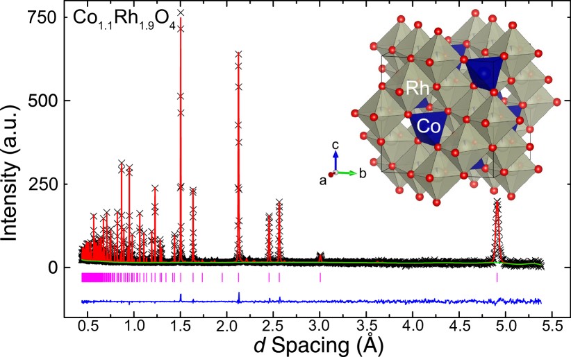
Figure 1: (Color online) Room temperature time-of-flight neutron powder diffraction (POWGEN) results for CoRh₂O₄. Experimental observations are indicated by black crosses and the results of Rietveld refinements as thin lines. Vertical pink ticks indicate expected peak position and solid blue line the difference between observations and refinements. The inset depicts the crystal structures of CoRh₂O₄ with O represented as red spheres, Rh octahedral with gray faces and Co tetrahedral with blue faces.

We start our experimental investigation by presenting the ideal diamond-lattice crystal structure of CoRh₂O₄. This material crystallizes in the cubic spinel structure [Fig. 1] with space group $Fd\bar{3}m$ and room-temperature structural parameters reported in Tab. 1. With respect to the general spinel structure AB₂O₄, Co²⁺ occupies the tetrahedrally coordinated A-site and Rh³⁺ the octahedrally coordinated B-site. This results in a perfect diamond lattice for the Co²⁺ ions with four nearest-neighbor Co atoms at a distance of $3.682$ Å. Nearest-neighbor magnetic exchange interactions are mediated by direct exchange or more likely by Co–O–Rh–O–Co superexchange paths Blasse (1963). Next-nearest-neighbor exchanges, if present, involve twelve equivalent superexchange pathways with Co–Co distances of $6.013$ Å.

Co1.1Rh1.9O4 [ $\equiv$ CoRh2O4 ], $T=300$ K
$Fd\bar{3}m,a\!=\!8.503(1)\mathrm{\AA},V\!=\!614.7(1)\mathrm{\AA}^{3},\chi^{2}\!=\!4.16,R_{\mathrm{wp}}\!=\!2.86\%$
Atom	Site	${x}$	${y}$	${z}$	Occ.	${U}_{{\rm iso}}$(Å2)
Co	$8a$	0	0	0	1.0	0.0021(2)
Rh	$16d$	5/8	5/8	5/8	0.95(6)	0.0002(1)
Co	$16d$	5/8	5/8	5/8	0.05(6)	0.0002(1)
O	$32e$	0.2601(1)	0.2601	0.2601	1.0	0.0023(1)

Table 1: Crystallographic parameters of CoRh₂O₄ obtained by neutron powder diffraction at room temperature.

The results of our refinement are consistent with previous reports Bertaut et al. (1959); Cascales and Rasines (1984) with two notable differences. First, the RhO₆ octahedral are less distorted in our structure compared to previous reports; the shortened (respectively elongated) Co–O (respectively Rh–O) bonds lead to more chemically-reasonable bond-valence sums Brown (1981) of 1.79 for Co and 3.05 for Rh. Second, our refinements indicate a small degree of site mixing with 5.0(6)% of Co on the B-site and formally, a refined chemical formula of CoRh_1.90(1)Co_0.10(1)O₄. The Rh deficiency originates from the presence of a small Rh₂O₃ impurity phase. To maintain overall charge balance, either octahedral Co ions are $3+$, i.e. Rh(III)_1.9Co(III)_0.1, or approximatively 5% of the Rh ions are $4+$, i.e. Rh(III)_1.8Rh(IV)_0.1Co(II)_0.1. Since the ionic radii for either scenario are similar it is not possible to favor one scenario over the other based on structural refinements alone. Although formally Co_1.1Rh_1.9O₄, we refer to our compound as CoRh₂O₄ in the rest of this manuscript.

III.2 Thermo-magnetic properties

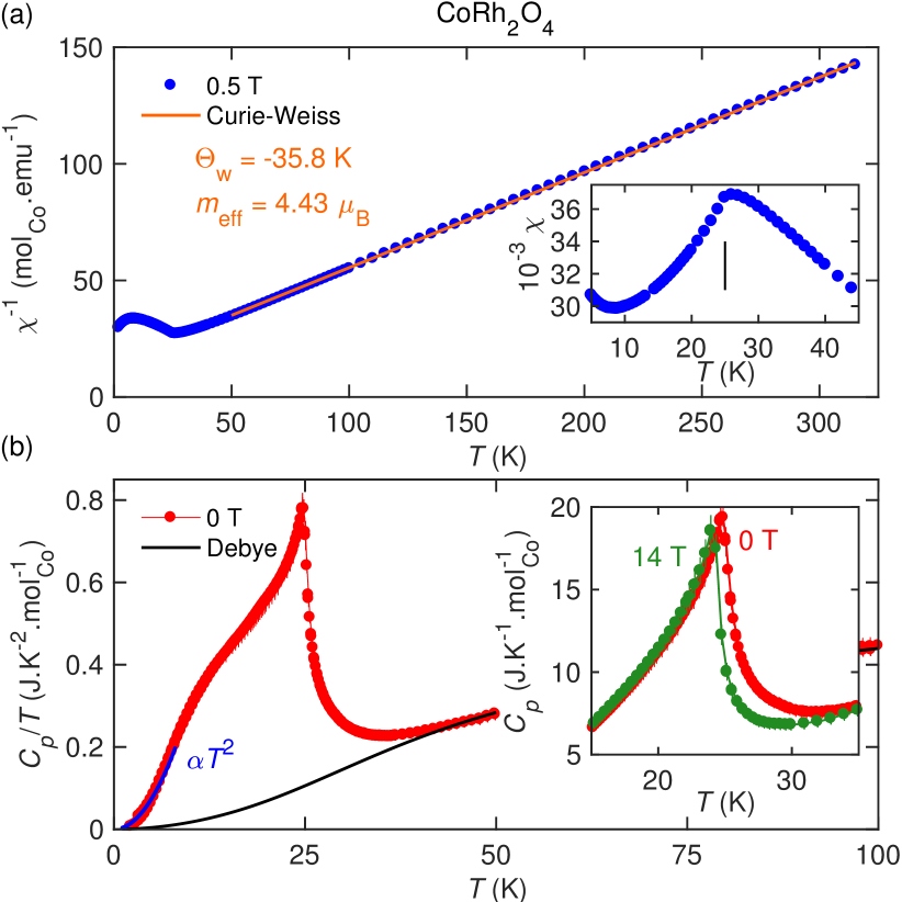
Figure 2: (Color online) Magnetic and thermal measurements for CoRh₂O₄. (a) Inverse magnetic susceptibility $\chi(T)^{-1}$ in an applied magnetic field of $\mu_{0}H=0.5$ T (blue circles) and Curie-Weiss fit (orange line). The temperature dependence of the magnetic susceptibility $\chi(T)$ is plotted as inset with an inflection point (black vertical line) associated with the Néel ordering transition. (b) Temperature dependence of the total specific heat divided by temperature $C_{p}(T)/T$ in zero magnetic field (red circles) and Debye fit (black line) indicating the lattice contribution. The field dependence of the specific heat $C_{p}(T)$ around its maximum is plotted as an inset (red circles for $\mu_{0}H\!=\!0$ T field and green circles for $\mu_{0}H\!=\!14$ T).

Magnetic and thermodynamic measurements for CoRh₂O₄ are presented in Fig. 2. The inverse magnetic susceptibility $1/\chi(T)$ [Fig. 2(a)] is linear over a broad range of temperatures $30\leq\!T\!\leq 300$ K. A Curie-Weiss fit to the high-temperature paramagnetic regime ($T\!\geq\!50$ K) yields a negative Weiss temperature $\Theta_{\mathrm{W}}=-35.8(4)$ K and an effective moment $\mu_{\rm eff}\!=\!4.43(1)$ $\mu_{\rm B}$, consistent with previous reports. Blasse and Schipper (1963); Blasse (1963) In the undistorted tetrahedral crystal-field environment, Co²⁺ adopts the $e_{g}^{4}t_{2g}^{3}$ electronic configuration with one unpaired electron in each $d_{xy}$, $d_{xz}$ and $d_{yz}$ orbitals. Bertaut et al. (1959) For such $S=3/2$ magnetic moments, the experimental value of $\mu_{\rm eff}$ yields a gyro-magnetic ratio $g\!\approx\!2.18$ after correcting for the presence of $1.1$ Co atoms per formula unit. At low temperatures, the magnetic susceptibility $\chi(T)$ [Fig. 2(a)-inset] displays a sharp absolute maximum closely followed by an inflection point at $T_{\rm N}=25.0$ K, attributed to long-range antiferromagnetic ordering. Blasse and Schipper (1963); Blasse (1963); Fiorani and Viticoli (1979)

These results are fully corroborated by heat-capacity measurements. The specific heat of CoRh₂O₄, plotted as $C_{p}/T$ [Fig. 2(b)], shows a sharp $\lambda$-shaped anomaly at $T_{\rm N}=25.68$ K, indicative of a second-order phase transition. The precise correspondence between specific heat and magnetic susceptibility leaves no doubt as to its magnetic nature. Most of the specific heat above $T\!\approx\!1.5\cdot T_{\rm N}$ can be accounted for by a phonon model with two Debye temperatures, $\Theta_{\rm D}={253(3)}$ K and 742(9) K. Integrating the magnetic part of $C_{p}/T$ from 1.7 K to 50 K yields an entropy change $\Delta S\!\approx\!11.7$ J.K^-1.mol^-1, consistent with $R\ln 4\!=\!11.52$ J.K^-1.mol^-1 expected for $S\!=\!3/2$ degrees of freedom. Below $T_{\rm N}$, the magnetic contribution to the specific heat dominates and a broad feature is observed around $T^{*}\!\approx\!12$ K, which we attribute to magnon-magnon interactions. Below $T^{*}$, the specific heat follows a $C_{p}\!=\!\alpha T^{3}$ behavior, as expected for gapless antiferromagnetic magnons. Given the relatively large energy scale set by $\Theta_{\mathrm{W}}\!\approx\!35$ K, a large applied magnetic field of $\mu_{0}H\!=\!14$ T has almost no influence on the transition temperature. We observe a shift downward by a mere $0.74$ K [Fig. 2(b)-inset]. Overall, our measurements yield a frustration ratio Ramirez (1994) $f\!=\!|\Theta_{\rm W}|/T_{\rm N}\!=\!1.4$ and suggest that CoRh₂O₄  behaves as a canonical non-frustrated three-dimensional antiferromagnet with an average exchange interaction between nearest-neighbor magnetic moments ($z\!=\!4$) of $J_{\rm av}\!=\!3k_{\rm B}\Theta_{\rm W}/zS(S+1)\!=\!0.62$ meV.

III.3 Magnetic structure

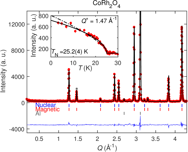
Figure 3: (Color online) Neutron powder diffraction (HB-2A) pattern of CoRh₂O₄ measured at $T\!=\!4$ K with a neutron wave-length of $\lambda=2.41$ Å  (red circles), and corresponding Rietveld refinements (black line) of the nuclear (blue ticks), magnetic (red ticks) and aluminum background (gray ticks) contributions. The blue line shows the difference between data and the best Rietveld fit for which peak shapes were modeled using a pseudo-Voigt function. The inset shows the temperature dependence of the most intense magnetic peak (highlighted with an asterisk). The black solid (respectively dot-dashed) curve is an order parameter fit with a fixed mean-field (3+1D) Ising (resp. Heisenberg) critical exponent $\beta=0.25$ (resp. $\beta=0.34$) in order to estimate the value of $T_{\rm N}$.

Neutron powder diffraction allows one to determine the magnetic structure of CoRh₂O₄ below the antiferromagnetic ordering transition at $T_{\rm N}\approx 25$ K [Fig. 3]. Upon cooling our sample from 40 K to 4 K, we observe a sizable change of intensity for some of the nuclear Bragg peaks, coinciding with the development of new Bragg peaks at nuclear positions forbidden by the space-group symmetry, for instance $\{h,k,\ell\}=\{2,0,0\}$ ($Q^{*}\!=\!1.47$ Å^-1) and $\{2,4,0\}$ ($Q\!=\!3.30$ Å^-1). The integrated intensity of the $\{2,0,0\}$ peak [Fig. 3-inset] follows an order-parameter behavior with a sharp onset at $T_{\mathrm{N}}=25.2(4)$ K, in close correspondence with the thermodynamic anomalies. We thus associate the change in Bragg scattering with the development of long-range magnetic ordering.

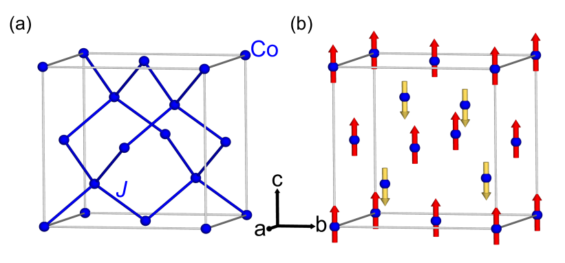
Figure 4: (Color online) Conventional body-centered unit cell for Co atoms (blue spheres) in CoRh₂O₄ showing (a) the diamond-lattice connectivity of the nearest neighbor bonds (blue lines) and (b) the two sublattice $\mathbf{k}_{\rm m}=(0,0,0)$ antiferromagnetic magnetic structure (red and yellow arrows) obtained from our Rietveld refinement.

All the observed magnetic Bragg peaks can be indexed by the magnetic propagation vector $\mathbf{k}_{\rm m}=(0,0,0)$ with respect to the conventional unit cell. To determine the magnetic structure, we first investigate possible symmetry-allowed magnetic structures using the program Isodistort. Campbell et al. (2006) For CoRh₂O₄, there are two irreducible representations (irreps), labeled $\Gamma_{4+}$ and $\Gamma_{5-}$ in the notation of Miller and Love. Miller and Love (1967) These correspond to simple ferromagnetic and antiferromagnetic ordered pattern on the diamond lattice [Fig. 4(a)], respectively. As anticipated from the negative Curie-Weiss constant, only $\Gamma_{5-}$ correctly accounts for the observed magnetic intensity. The resulting spin structure (magnetic space group $I4_{1}{{}^{\prime}}/a{{}^{\prime}}m{{}^{\prime}}d$) is shown in Fig. 4(b). Our Rietveld refinement [Fig. 3] is in excellent agreement with the data ($R_{\mathrm{wp}}\!=\!8.11\%,R_{\mathrm{mag}}\!=\!7.62\%$) and yields an ordered magnetic moment $\mu_{\mathrm{ord}}=3.11(5)\,\mu_{\mathrm{B}}$, close to the value of $gS=3.27\,\mu_{\mathrm{B}}$ expected for a $S=3/2$ ion with $g=2.18$. Neutron powder diffraction thus demonstrates that CoRh₂O₄ orders in a simple two-sublattice antiferromagnetic structure at $T_{\rm N}\!\approx\!25$ K and places an upper bound of 5% on any reduction of the ordered moment due to quantum fluctuations at $T\!=\!4$ K.

III.4 Magnetic excitations

Inelastic neutron scattering measurements on CoRh₂O₄ [Fig. 5(a)] reveal a simple magnetic excitation spectrum we associate with non-interacting magnons, i.e. spin fluctuations transverse to the ordered spin patterns of Fig. 4(b). The magnetic spectrum appears gapless within the resolution of our experiments, with characteristic acoustic spin-wave branches emerging from the strong magnetic Bragg peak positions. The bandwidth of the magnetic signal $W\approx 3.8$ meV = 44 K matches well with the value of the Weiss constant $\Theta_{\rm W}\!=\!35.5$ K and corresponds to the energy of magnons at the Brillouin zone boundary. We obtain an excellent correspondence between the data and the calculated scattering intensity [Fig. 5(b)] with a single nearest-neighbor exchange parameter $J_{1}\!=\!0.63$ meV [Fig. 4(b)]. This matches very well with the average exchange value extracted from the magnetic susceptibility $J_{\rm av}\!=0.62$ meV, indicating that further neighbor exchanges and $T\!=\!0$ magnon energy renormalization effects can be neglected in CoRh₂O₄.

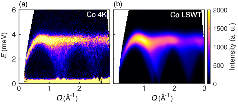
Figure 5: (Color online) Magnetic excitations of CoRh₂O₄. (a) Momentum and energy dependence of the powder inelastic neutron scattering intensity $I(Q,E)$ at $T=4$ K. (b) Linear spin-wave theory simulations of $I(Q,E)$, for the magnetic structure of Fig. 4(b), stabilized by a nearest-neighbor exchange interaction $J_{1}=0.63$ meV.

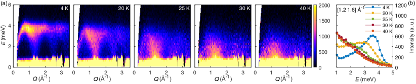
Figure 6: (Color online) Temperature dependence of the magnetic excitations of CoRh₂O₄. (a) Evolution of the $Q$–$E$ scattering intensity upon crossing $T_{\rm N}\approx 25$ K. (b) Constant-$Q$ cut around the ordering wave-vector position $Q^{*}=1.4\pm 0.2~{}$Å^-1.

The temperature dependence of the magnetic excitations [Fig. 6(a)] reveals a very rapid collapse of the magnetic excitations as $T_{\rm N}$ is crossed. Unlike low-dimensional quasi-1D and quasi-2D magnets for which the overall bandwidth and shape of the magnetic excitations persists at and above $T_{\rm N}$, Lake et al. (2005); Rønnow et al. (1999) the excitations of CoRh₂O₄ resemble that of a paramagnet already for $T\!\gtrapprox\!T_{\rm N}$. The top of the magnon band is considerably renormalized and broadened at $T=T_{\rm N}$ , a temperature above which the excitations loose coherence and the inelastic signal becomes purely relaxational [Fig. 6(b)]. While the detailed analysis of the temperature dependence of these excitations is beyond the scope of this work, the simplicity of the $T\ll T_{\rm N}$ spectrum and the presence of an unique energy scale $J_{1}\!=\!0.63$ meV makes CoRh₂O₄ a model 3D antiferromagnetic material.

IV Results on Copper Rhodite

IV.1 Structural analysis

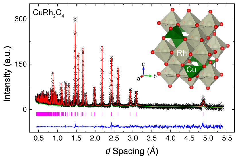
Figure 7: (Color online) Room temperature time-of-flight neutron powder diffraction (POWGEN) results for CuRh₂O₄. Experimental observations are indicated by black crosses and the results of Rietveld refinements as thin lines. Vertical pink thicks indicate expected peak position and solid blue line the difference between observations and refinements. The inset depicts the crystal structure of CuRh₂O₄ with O represented as red spheres, Rh octahedral with gray faces and Cu tetrahedral with green faces.

CuRh₂O₄ crystallizes in a lower-symmetry crystal structure than CoRh₂O₄ due to a Jahn-Teller distortion around $T_{\rm JT}\approx 850$ K Bertaut et al. (1959); Blasse (1963) lifting the degeneracy of the $e_{g}^{4}t_{2g}^{5}$ electronic configuration of Cu²⁺. The necessary destabilization of the magnetic $d_{xy}$ orbital below $T_{\rm JT}$ leads to a compression of the oxygen tetrahedral with respect to the cubic cell. Bertaut et al. (1959) Indeed the structure of CuRh₂O₄ has been described by both X-ray Khanolkar (1961) and neutron diffraction Ismunandar et al. (1999) as a tetragonally distorted spinel with space group $I4_{1}/amd$ Ismunandar et al. (1999) or $I\bar{4}2d$.Khanolkar (1961)

CuRh2O4, $T=300$ K
$I{4}_{1}/amd,a\!=\!6.177(1)\mathrm{\AA},c\!=\!7.902(1)\mathrm{\AA},V\!=\!301.5(1)\mathrm{\AA}^{3}$
$\chi^{2}\!=\!3.86,R_{\mathrm{wp}}\!=\!2.66\%$
Atom	Site	${x}$	${y}$	${z}$	Occ.	${U}_{{\rm iso}}$(Å2)
Cu	$8e$	0	3/4	0.1368(3)	1.0	0.0017(2)
Rh	$8d$	0	0	1/2	1.0	0.0005(1)
O	$16h$	0	0.0334(1)	0.2430(1)	1.0	-
Anisotropic Atomic Displacement Parameters (Å2)
Atom	${U}_{{11}}$	${U}_{{22}}$	${U}_{{33}}$	${U}_{{12}}$	${U}_{{13}}$	${U}_{{23}}$
O	0.0021	0.0010	0.0022	0.0	0.0	$0.0002$

Table 2: Crystallographic parameters of CuRh₂O₄ obtained by neutron powder diffraction at room temperature.

Our room temperature neutron diffraction results for CuRh₂O₄ are shown in Fig. 7. The results of our Rietveld refinement, reported in Table 2, yield $I4_{1}/amd$ as the appropriate room-temperature space group, consistent with the most recent studies. Ismunandar et al. (1999); Dollase and O’Neill (1997) Unlike CoRh₂O₄, we find no evidence for site mixing with bond valence sums of 3.05 for Rh, 1.97 for O and 1.79 for Cu. A close look at the crystal structure indicates that Rh octahedral are distorted with four distinct O—Rh—O bond angles of 98.23(4)^∘, 81.77(4)^∘, 92.83(5)^∘ and 87.17(5)^∘. In turn, the Cu tetrahedral are flattened with two distinct O—Cu—O bond angles of 128.8(2)^∘ and 102.6(1)^∘. For comparison, there are only two O-Rh-O angles of 85.10(3)^∘ and 94.90(3)^∘ and a single O-Cu-O angle of 109.47(3)^∘ in CoRh₂O₄. Our refined crystal structure also indicates Cu is displaced off the ideal $4a$ site in a disordered manner. Instead, the copper position splits between two $8e$ positions that are randomly occupied along the $c$ axis. Overall the tetragonal distortion leads to four nearest-neighbor Cu—Cu distances within $0.2\%$ of each other such that nearest-neighbor Cu²⁺ ions in CuRh₂O₄  effectively remain organized on a diamond lattice at an average distance of 3.61(5) Å. When compared to the cubic structure of CoRh₂O₄, however, next-nearest-neighbor Cu—Cu distances are strongly split into four short and eight long links. We will see below this has profound consequences for the magnetic properties of CuRh₂O₄.

IV.2 Thermo-magnetic properties

Magnetic and thermodynamic measurements for CuRh₂O₄ are presented in Fig. 8. Unlike CoRh₂O₄  the inverse magnetic susceptibility $1/\chi(T)$ [Fig. 8(a)] only becomes linear at high temperature after subtraction of a positive Van-Vleck contribution $\chi_{\rm VV}$, associated with paramagnetic Rh³⁺. Endoh et al. (1999) Linearity of $[\chi(T)-\chi_{\rm VV}]^{-1}$ for $T\geq 170$ K is obtained using $\chi_{\rm VV}=+200\times 10^{-6}$ emu.mol^-1 from which a Curie-Weiss fit yields $\Theta_{\mathrm{W}}=-132.2(7)$ K and $\mu_{\rm eff}\!=\!2.073(2)$ $\mu_{\rm B}$. The obtained effective moment is somewhat too large for Cu²⁺. Using an empirical $\chi_{\rm VV}=+400\times 10^{-6}$ emu.mol^-1, we obtain a good Curie-Weiss fit above $T\geq 120$ K with values of $\Theta_{\mathrm{W}}=-93(1)$ K and $\mu_{\rm eff}\!=\!1.819(5)$ $\mu_{\rm B}$, compatible with a previous report Endoh et al. (1999) and corresponding to a realistic gyro-magnetic ratio $g\!\approx\!2.1$ for the Cu²⁺ ions. At low temperatures, the magnetic susceptibility $\chi(T)$ [Fig. 8-inset] displays a local maximum with an inflection point at $T_{\rm N}\!=\!23.5$ K, indicating antiferromagnetic ordering. Endoh et al. (1999)

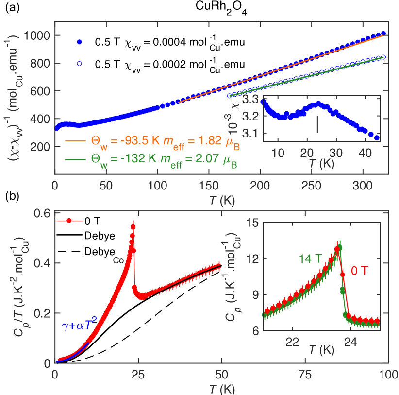
Figure 8: (Color online) Magnetic and thermal measurements for CuRh₂O₄. (a) Inverse magnetic susceptibility $(\chi(T)-\chi_{\rm VV})^{-1}$ in an applied magnetic field of 0.5 T with two distinct temperature-independent Van-Vleck contributions $\chi_{\rm VV}$ subtracted (solid and empty blue circles) and corresponding Curie-Weiss fits (orange and green lines, respectively). Temperature dependence of the total specific heat divided temperature $C_{p}(T)/T$ in zero magnetic field (red circles) and fits to the lattice contribution of CuRh₂O₄ (black line) and CoRh₂O₄ (dashed line). The field dependence of the specific heat $C_{p}(T)$ around its maximum is plotted as inset (red circles for $\mu_{0}H=0$ T field and green circles for $\mu_{0}H=14$ T.

The specific heat of CuRh₂O₄ [Fig. 8(b)] displays a sharp $\lambda$-shaped peak at $T_{\rm N}\!=\!23.54$ K in perfect correspondence with the susceptibility result. This peak shifts by less than $0.1$ K when a magnetic field of $\mu_{0}{\it H}\!=\!14$ T is applied [Fig. 8(b)-inset]. A phonon model with two Debye temperatures, $\Theta_{\rm D}=116(12)$ K and $350(14)$ K, accounts for most of the specific heat for $T\geq 1.5\cdot T_{\rm N}$ but overestimates the phonon contribution as the entropy change from 1.7 K to 50 K, $\Delta S\!\approx\!3.2$ J.K^-1.mol^-1, falls short of $R\ln 2\!=\!5.76$ J.K^-1.mol^-1 expected for $S\!=\!1/2$ degrees of freedom. Using the Debye model from CoRh₂O₄  the magnetic entropy reaches $\Delta S\!\approx\!6.5$ J.K^-1.mol^-1 at 50 K, the large value of which suggests possible magneto-elastic effects. Below $T\leq 20$ K, the specific heat is well described by $C_{p}\!=\!\gamma T+\alpha T^{3}$, where the small $\gamma\!=\!5\times 10^{-3}$ J.K^-2.mol^-1 term may indicate weak glassiness in the low energy spectrum of otherwise gapless antiferromagnetic magnons. The large $\Theta_{\rm W}$ compared to $T_{\rm N}$ suggests a moderate degree of frustration in CuRh₂O₄, with $4.0\!\leq\!f\!\leq\!5.5$. In the following, we investigate the nature and consequences of competing (frustrated) exchange interactions in CuRh₂O₄.

IV.3 Magnetic structure

More direct evidence for the presence of frustration in CuRh₂O₄ comes from low-temperature neutron diffraction. After cooling our sample of CuRh₂O₄ from 25 K to 4 K [Fig. 9], we observed new Bragg peaks at small wave-vectors ($Q\lesssim 2$ Å^-1). Given the known thermodynamic anomalies, we identify these peaks with the development of long-range magnetic order. As anticipated for a $S\!=\!1/2$ system, these magnetic Bragg peaks are very weak. In fact, we observed only a single magnetic peak above background (at $Q=1.04$ Å^-1) in our diffraction data taken with $\lambda=2.41$ Å and optimized for high resolution. The temperature dependence of the integrated intensity of this peak [Fig. 9-inset] yields $T_{\mathrm{N}}=24(1)$ K. However, we were able to observe several magnetic Bragg peaks with good statistics by integrating our inelastic scattering data over the elastic energy resolution [Fig. 9], which we will henceforth refer to as “elastic scattering”.

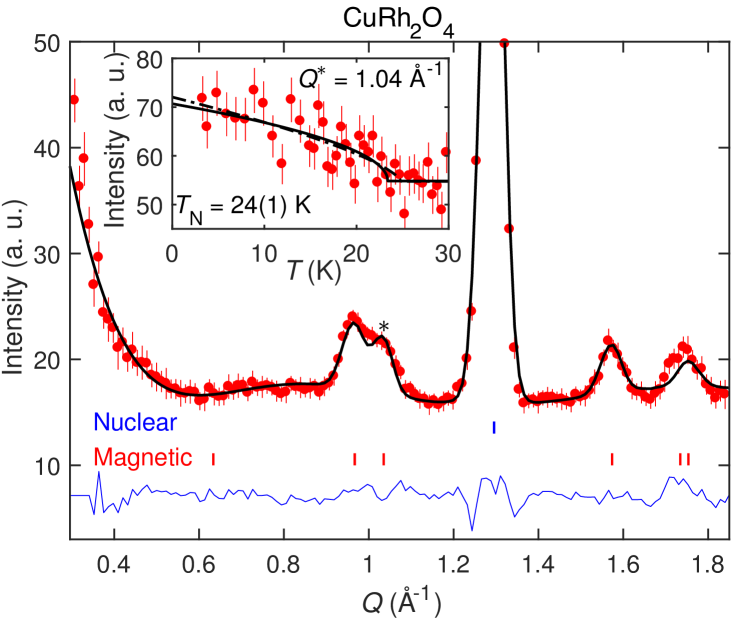
Figure 9: (Color online) Rietveld refinement of our CuRh₂O₄ elastic scattering results at $T\!=\!4$ K, extracted from an $E$-integrated elastic cut through our inelastic data (SEQUOIA). Nuclear (blue ticks) and magnetic (red ticks) phases are included. The inset shows the temperature dependence of one of the most intensive magnetic peak (highlighted with asterisk) obtained by neutron diffraction (HB-2A). The black solid (respectively dot-dashed) curve is an order parameter fit with a fixed mean-field (3+1D) Ising (resp. Heisenberg) critical exponent $\beta=0.25$ (resp. $\beta=0.344$) in order to estimate the value of $T_{\rm N}$.

The magnetic Bragg peaks are indexed by an incommensurate magnetic propagation vector $\mathbf{k}_{\rm m}=(0,0,k_{z})$ with respect to the conventional unit cell, where $k_{z}\!\approx\!0.79$. For the space-group of CuRh₂O₄ and $\mathbf{k}_{\rm m}$, there are three irreps, of which two are one-dimensional, $\Lambda_{3}$ and $\Lambda_{4}$, and one is two-dimensional, $\Lambda_{5}$. Campbell et al. (2006) However, the one-dimensional irreps can be discounted, because they correspond to amplitude-modulated spin-density waves with the ordered magnetic moment parallel to the $\mathbf{c}$ axis of the tetragonal unit cell, which would lead to the $\{0,0,2-k_{z}\}$ Bragg peak ($Q\!=\!0.962$ Å^-1) being absent, in conflict with experimental observations. The $\Lambda_{5}$ irrep corresponds to the ordered spin component lying in the $ab$ plane and it contains two candidate magnetic structures for which all spins possess ordered magnetic moments of equal magnitude. Both structures are circular helices ($\mathbf{k}_{\rm m}$ perpendicular to the spins’ plane of rotation), with the angle $\varphi$ between adjacent spins along ${\bf c}$ given by $\cos\varphi=\pm 0.32$. Calculating the powder-diffraction patterns reveals that only the structure with $\cos\varphi\!=\!-0.32$ shows good agreement with experimental data. We therefore identify the magnetic structure of CuRh₂O₄ as a circular helix with $\cos\varphi\!=\!-0.32$. This structure (magnetic space group $I4_{1}221^{\prime}$), which probably originates from competing exchange interactions [Fig. 10(a)], is shown in Fig. 10(b).

We performed Rietveld refinements against our neutron data to obtain accurate values for $k_{z}$ and the ordered magnetic moment length $\mu_{\mathrm{ord}}$. Because the elastic data have high statistics but relatively low resolution, while the opposite is true of the diffraction data, we fit to several datasets simultaneously; namely, the $4-25$ K elastic data (magnetic phase), the $4$ K elastic data (magnetic and nuclear phases), the $4-25$ K diffraction data (magnetic phase), and the $4$ K diffraction data (nuclear phase). The magnetic phase was excluded from the fit to the $4$ K diffraction data because of additional weak peaks from the sample environment, which may bias the magnetic refinement. The fit to the 4 K elastic data [Fig. 9] represents good agreement with the data ($R_{\mathrm{wp}}=6.53\%;R_{\mathrm{mag}}=18.8\%$). The refined parameter values are $k_{z}\!=\!0.790(4)$ and $\mu_{\mathrm{ord}}\!=\!0.56(6)\,\mu_{\mathrm{B}}$. The value of $\mu_{\mathrm{ord}}$ is significantly reduced from its maximum expected value of $1.05\,\mu_{\mathrm{B}}$, which indicates strong quantum fluctuations, an effect we consider in detail below.

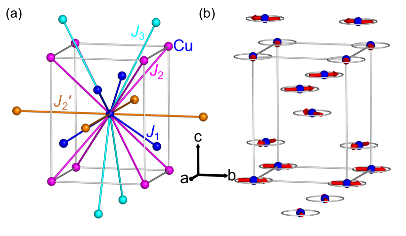
Figure 10: Conventional body-centered unit cell for Cu atoms (colored spheres) in CuRh₂O₄ showing (a) the connectivity of the nearest neighbor (blue lines), second neighbor (pink and orange lines), and third neighbor bonds (cyan lines). The two distinct kinds of second neighbor interactions are degenerate in the cubic case. (b) Incommensurate magnetic structure of CuRh₂O₄ with $\mathbf{k}_{\rm m}=(0,0,0.79)$ and $\cos\varphi=-0.32$.

IV.4 Magnetic excitations

CuRh2O4	$J_{1}=10.1$ meV	$J_{2}=0.32~{}J_{1}$
	$J_{3}=0.098~{}J_{1}$	$J^{\prime}_{2}=0.18~{}J_{1}$

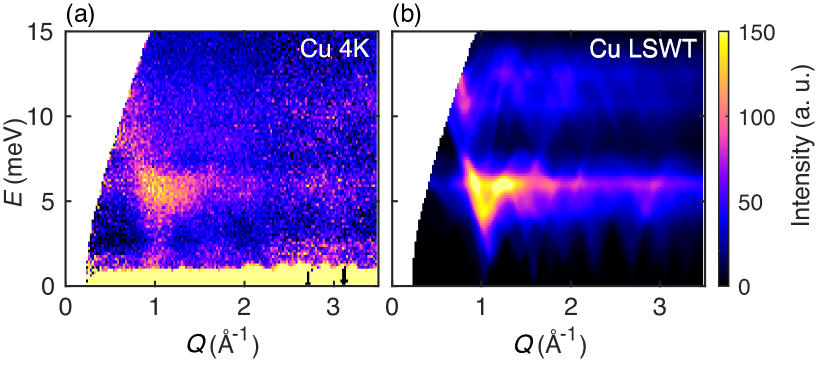
Figure 11: (Color online) Magnetic excitations of CuRh₂O₄. (a) Momentum and energy dependence of the powder inelastic neutron scattering intensity $I(Q,E)$ at $T=4$ K. (b) Linear spin-wave theory simulations of $I(Q,E)$, for the magnetic structure of Fig. 10(b), stabilized by the magnetic exchange interactions listed above the plot and defined in Fig. 10(a).

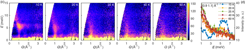
Figure 12: (Color online) Temperature dependence of the magnetic excitations of CuRh₂O₄. (a) Evolution of the $Q$–$E$ scattering intensity upon crossing $T_{\rm N}\approx 23$ K. (b) Constant-$Q$ cut around the ordering wave-vector position $Q=1.0\pm 0.1~{}$Å^-1.

To explain the origin of this incommensurate magnetic structure, we resort to inelastic neutron scattering to determine the values of possible magnetic exchange interactions for the distorted structure of CuRh₂O₄ [Fig. 10(a)]. The magnetic spectrum of CuRh₂O₄ appears gapless within the resolution of our experiments but unlike CoRh₂O₄ we observe a complex landscape of high-energy excitations, with peaks in the density of magnetic scattering at $W_{1}\!=\!6.2\!$ meV and $W_{2}\!\approx\!11.5\!$ meV, several times greater than the excitation bandwidth of CoRh₂O₄. Given that the nearest-neighbor magnetic ion distances are very similar for the two compounds (3.68 Å and 3.61 Å), this suggests super-exchange interactions very sensitive to the details of the crystal structure. Furthermore, the presence of two apparent energy scales in CuRh₂O₄ implies that several exchange interactions exist, and potentially compete, to stabilize the incommensurate magnetic structure.

To model the excitations of CuRh₂O₄, we consider a Heisenberg model with up to third-nearest neighbor interactions; see Fig. 10(a). The nearest-neighbor interaction $J_{1}$ defines a diamond lattice as in the cubic case. The next-nearest neighbor interaction, however, splits from a face-centered cubic connectivity into distinct $J_{2}$ and $J_{2}^{\prime}$ interactions that define body-centered and square networks, respectively. In turn, the third-neighbor interaction $J_{3}$ forms a diamond lattice. This model yields a large parameter space; we defer the study of its mean-field phase diagram and role of quantum fluctuations to Sec. V. With the propagation vector $\mathbf{k}_{\rm m}$ and the inelastic spectrum as a constraints, we obtain an excellent match between the data and the calculated scattering intensity for $J_{1}=10.1$ meV, $J_{2}/J_{1}=0.32$, $J_{2}^{\prime}/J_{1}=0.18$ and $J_{3}/J_{1}=0.098$ [Fig. 11]. As we will see below, this set of parameters is uniquely constrained by the experimental data. We note that in the cubic case, the average value $(J_{2}+J_{2}^{\prime})/2J_{1}=0.125$ would yield a highly degenerate coplanar spiral state. Bergman et al. (2007) The Jahn-Teller distortion in CuRh₂O₄ is thus crucial to stabilize a well-defined spin-helix with a unique propagation vector $\mathbf{k}_{\rm m}=(0,0,0.79)$. In a trend already observed for CoRh₂O₄, the temperature dependence of the magnetic excitations of CuRh₂O₄ [Fig. 12] is marked by a very rapid collapse of the magnetic bandwidth as $T_{\rm N}$ is crossed.

V Theoretical analysis

V.1 Mean-field phase diagram

In this section we apply mean-field theory to relate the magnetic structure of CuRh₂O₄ to a Heisenberg Hamiltonian with the exchange interactions of Fig. 10(a). Calculations are efficiently performed in a primitive unit cell, which is less symmetric than the conventional cell but contains the smallest possible number of atoms; see Appendix A. We proceed with the Heisenberg model,

$$\mathcal{H}=\frac{1}{2}\sum_{i,j,m,n}J_{ij}(\mathbf{R}_{n}-\mathbf{R}_{m})\,\mathbf{S}_{i}(\mathbf{R}_{m})\cdot\mathbf{S}_{j}(\mathbf{R}_{n}),$$ (1)

where $\mathbf{S}_{i}(\mathbf{R}_{m})$ denotes the $i$-th spin of a primitive unit cell located at a lattice vector $\mathbf{R}_{m}$ from the origin, and $J_{ij}(\mathbf{R}_{n}-\mathbf{R}_{m})\equiv J_{d}$ is the exchange interaction between spins $\mathbf{S}_{i}(\mathbf{R}_{m})$ and $\mathbf{S}_{j}(\mathbf{R}_{n})$. We consider the four exchange interactions $J_{1}$, $J_{2}$, $J_{2}^{\prime}$ and $J_{3}$ shown in Fig. 10(a) and neglect possible exchange anisotropies.

Our mean-field theory follows the steps of Bertaut Bertaut (1962) and Chapon Chapon (2009) and proceeds by taking the Fourier transform of the exchange interactions,

$$J_{ij}(\mathbf{q})=\sum_{n}J_{ij}(\mathbf{R}_{n})\exp\left(-\mathrm{i}\mathbf{q}\cdot\mathbf{R}_{n}\right),$$ (2)

where $i\in\left\{1,2\right\}$ labels the two Cu ions in the primitive unit cell. $J_{ij}(\mathbf{q})$ describes a $2\times 2$ Hermitian matrix for each momentum $\mathbf{q}$ in the first Brillouin zone,

$$J(\mathbf{q})=-\left(\begin{array}[]{cc}J_{11}&J_{12}\\ J_{12}^{*}&J_{11}\end{array}\right),$$ (3)

where $J_{ij}^{*}(\mathbf{q})=J_{ij}(-\mathbf{q})$. The matrix elements are evaluated by identifying the lattice translation vectors that connect pairs of spins dressed by a given interaction. Using Eq. (A) to convert from primitive to conventional indices, we obtain

$$J_{11}(\mathbf{q}) = 2J_{2}\{\cos\left[\pi\left(h+k+l\right)\right]+\cos\left[\pi\left(h+k-l\right)\right]$$ (4)

$$~{}~{}~{}~{}~{}+\cos\left[\pi(k+l-h)\right]+\cos\left[\pi\left(h+l-k\right)\right]\}$$

$$+ 2J^{\prime}_{2}\left[\cos\left(2\pi h\right)+\cos\left(2\pi k\right)\right],$$

$$J_{12}(\mathbf{q}) = J_{1}\large\{1+e^{2\pi ik}+e^{\pi i\left(h+k+l\right)}+e^{\pi i\left(-h+k+l\right)}\large\}$$

$$+ J_{3}\large\{e^{-\pi i\left(h-k+l\right)}+e^{\pi i\left(h+k-l\right)}+e^{2\pi il}+e^{2\pi i\left(k+l\right)}\large\},$$

where $(h,k,l)$ are expressed in reciprocal lattice units of the conventional unit cell.

The interaction matrix has two eigenvalues at each wavevector $\mathbf{q}$, given by

$$\lambda_{\pm}(\mathbf{q})=J_{11}(\mathbf{q})\pm\left|J_{12}(\mathbf{q})\right|.$$ (6)

The wavevector $\mathbf{k}$ for which $\max\left[\lambda_{\pm}(\mathbf{k})\right]$ reaches a global maximum in the first Brillouin zone is associated with the propagation vector $\mathbf{k}_{\rm m}$ of the ordered magnetic state. Only a small number of $\mathbf{k}$ points related by symmetry usually fulfill this condition. Highly-frustrated systems are exceptions for which $\max\left[\lambda(\mathbf{q})\right]$ can be degenerate over large regions of the Brillouin zone. Reimers et al. (1991) Given the large parameter space, a systematic search for maximum eigenvalues as a function of $J_{1}$, $J_{2}$, $J_{2}^{\prime}$ and $J_{3}$ is very time consuming. Minimization of the classical ground-state energy can significantly reduce the computing burden by providing analytical solutions for the magnetic structure, see Appendix B.

Our mean-field phase diagram as a function of $J_{2}/J_{1}$ and $J_{2}^{\prime}/J_{1}$ for different values of $J_{3}$ and assuming all exchanges antiferromagnetic is shown in Fig. 13. As well as of the Néel phase, we identify three different incommensurate phases for which the magnetic propagation vector takes the form $\mathbf{k}_{{\rm m},1}\!=\!(\xi,\xi,0)$, $\mathbf{k}_{{\rm m},2}\!=\!(\xi,0,0)$ (which is equivalent to $(0,\xi,0)$) or $\mathbf{k}_{{\rm m},3}\!=\!(0,0,\xi)$. The propagation vector observed for CuRh₂O₄, $\mathbf{k}_{{\rm m},3}$, is stabilized with an incommensurate $\xi$ value for a broad range of $J_{2}/J_{1}$ and $J_{2}^{\prime}/J_{1}$ values. A large $J_{3}/J_{1}$, however, pins the spiral to the lattice and leads to $\mathbf{k}_{{\rm m},3}\!=\!(0,0,1)$. Critically, our results indicate that the value of $\mathbf{k}_{{\rm m},3}$ is only affected by $J_{2}/J_{1}$ and $J_{3}/J_{1}$ but not by $J^{\prime}_{2}/J_{1}$. Therefore, the experimentally-measured value of the propagation vector constraints the ratio of $J_{3}/J_{1}$ to $J_{2}/J_{1}$, which eliminates one degree of freedom when simulating the excitations of CuRh₂O₄ with linear spin wave theory.

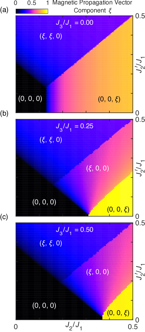
Figure 13: Mean-field phase diagrams for the CuRh₂O₄ Hamiltonian of Fig. 10(a) with different $J_{2}/J_{1}$, $J_{2}^{\prime}/J_{1}$ and $J_{3}/J_{1}$. The color represents the free components of the magnetic propagation vector in the different phases we uncover.

V.2 Linear spin-wave theory

With the knowledge of the possible magnetic structures of the model, we resort to linear spin-wave theory to simulate the dynamics of spins in both coumpounds and to refine further the exchanges parameters for CuRh₂O₄ [Fig. 10(a)]. For CoRh₂O₄ we only consider the nearest-neighbor coupling. While the simulated scattering intensities of Figs. 5 and 11 are obtained numerically using SpinW, (Toth and Lake, 2015) we proceed below with the explicit calculation of the magnon dispersion, a step necessary to calculate the effect of zero-point quantum fluctuations on the magnetic ordering.

We start with the general case of CuRh₂O₄ for which we set the spins to lie in the $x_{0}$-$y_{0}$ plane of the laboratory reference frame (the conventional unit cell). In order to align the quantization axis $z$ along the direction of each spin, we perform the following transformation,

$$S_{i}^{x_{0}}(\mathbf{R}_{n})=-S_{i}^{y}(\mathbf{R}_{n})\sin\theta+S_{i}^{z}(\mathbf{R}_{n})\cos\theta,$$ (7)

$$S_{i}^{y_{0}}(\mathbf{R}_{n})=-S_{i}^{y}(\mathbf{R}_{n})\cos\theta-S_{i}^{z}(\mathbf{R}_{n})\sin\theta,$$ (8)

$$S_{i}^{z_{0}}(\mathbf{R}_{n})=S_{i}^{x}(\mathbf{R}_{n}),$$ (9)

where $\theta$ is related to the propagation vector $\mathbf{k}_{\rm m}$ and is a function of $i$ and $\mathbf{R}_{n}$. We then introduce the Holstein-Primakoff $a$-bosons, which to linear order relate to spin operators in the rotating frame as

$$S_{i}^{z}(\mathbf{R}_{n}) = S-a_{i,\mathbf{R}_{n}}^{\dagger}a_{i,\mathbf{R}_{n}},$$ (10)

$$S_{i}^{x}(\mathbf{R}_{n}) \approx \sqrt{S/2}(a_{i,\mathbf{R}_{n}}+a_{i,\mathbf{R}_{n}}^{\dagger}),$$ (11)

$$S_{i}^{y}(\mathbf{R}_{n}) \approx -i\sqrt{S/2}(a_{i,\mathbf{R}_{n}}-a_{i,\mathbf{R}_{n}}^{\dagger}),$$ (12)

and Fourier transform as

$$a_{i,\mathbf{R}_{n}}=\sum\limits_{\mathbf{q}\in\mathrm{B.Z.}}a_{i,\mathbf{q}}e^{i\mathbf{q}\cdot\mathbf{R}_{n}}.$$ (13)

Keeping only quadratic terms in boson operators, we obtain the Hamiltonian

$$\hat{\mathcal{H}}_{2}=\frac{1}{2}\sum\limits_{\mathbf{q}\in\mathrm{B.Z.}}\bm{X}_{\mathbf{q}}^{\dagger}H_{\mathbf{q}}\bm{X}_{\mathbf{q}},$$ (14)

where $\bm{X}_{\mathbf{q}}^{\dagger}\equiv(a_{1,\mathbf{q}}^{\dagger},a_{2,\mathbf{q}}^{\dagger},a_{1,-\mathbf{q}},a_{2,-\mathbf{q}})$ is a row vector of boson operators and $\bm{X}_{\mathbf{q}}$ the corresponding column vector. In this representation, $H_{\mathbf{q}}$ is a $4\times 4$ Hermitian matrix which can be diagonalized provided the following bosonic commutation rules are preserved:

$$g=\bm{X}_{\mathbf{q}}\bm{X}_{\mathbf{q}}^{\dagger}-\bm{X}_{\mathbf{q}}^{\ast}\bm{X}_{\mathbf{q}}^{\rm{T}}=\left(\begin{array}[]{cccc}1&0&0&0\\ 0&1&0&0\\ 0&0&-1&0\\ 0&0&0&-1\end{array}\right).$$ (15)

For the $\mathbf{k}_{m,3}=(0,0,\xi)$ magnetic structure observed in CuRh₂O₄, the matrix elements $\{h_{ij}\}$ of $H_{\mathbf{q}}$ read:

$$h_{11} =h_{22}=h_{33}=h_{44}=$$ (16)

$$-4S\big{[}J_{1}\cos\varphi+2J_{2}\cos\gamma+J_{2}^{\prime}-J_{2}^{\prime}\zeta_{2^{\prime}}(\mathbf{q})$$

$$-J_{2}(1+\cos\gamma)\zeta_{2}(\mathbf{q})+J_{3}\cos 3\varphi\big{]},$$

$$h_{12} =h_{34}=$$ (17)

$$2S\big{[}J_{1}(1+\cos\varphi)\zeta_{1}(\mathbf{q})+J_{3}(1+\cos 3\varphi)\zeta_{3}(\mathbf{q})\big{]},$$

$$h_{13} =h_{31}=h_{24}=h_{42}=$$ (18)

$$4SJ_{2}(1-\cos\gamma)\zeta_{2}(\mathbf{q}),$$

$$h_{14} =h_{32}=$$ (19)

$$2S\big{[}J_{1}(1-\cos\varphi)\zeta_{1}(\mathbf{q})+J_{3}(1-\cos 3\varphi)\zeta_{3}(\mathbf{q})\big{]},$$

$$h_{21} =h_{43}=$$ (20)

$$2S\big{[}J_{1}(1+\cos\varphi)\zeta^{\ast}_{1}(\mathbf{q})+J_{3}(1+\cos 3\varphi)\zeta^{\ast}_{3}(\mathbf{q})\big{]},$$

$$h_{23} =h_{41}=$$ (21)

$$2S\big{[}J_{1}(1-\cos\varphi)\zeta^{\ast}_{1}(\mathbf{q})+J_{3}(1-\cos 3\varphi)\zeta^{\ast}_{3}(\mathbf{q})\big{]},$$

where $\zeta_{i}(\mathbf{q})$’s are the lattice harmonics associated with exchange $J_{i}$,

$$\zeta_{1}(\mathbf{q}) =$$ (22)

$$\frac{1}{4}\left(1+e^{-i\pi(-h+k+l)}+e^{-i2\pi k}+e^{-i\pi(h+k+l)}\right),$$

$$\zeta_{2^{\prime}}(\mathbf{q}) =\frac{1}{2}\Big{(}\cos[2\pi k]+\cos[2\pi h]\Big{)},$$ (23)

$$\zeta_{2}(\mathbf{q}) =\frac{1}{4}\Big{(}\cos[\pi(-h+k+l)]+\cos[\pi(h-k+l)]$$ (24)

$$~{}~{}~{}~{}~{}+\cos[\pi(h+k-l)]+\cos[\pi(h+k+l)]\Big{)},$$

$$\zeta_{3}(\mathbf{q}) =$$ (25)

$$\frac{1}{4}\Big{(}e^{i\pi(h-k+l)}+e^{-i\pi(h+k-l)}+e^{-2i\pi l}+e^{-2i\pi(k+l)}\Big{)},$$

with $\mathbf{q}=(h,k,l)$ in reciprocal lattice units of the conventional unit cell.

In general, it is not possible to give an analytical form for the above eigenvalue problem. We thus follow the numerical solution described by S. Petit. Petit, S (2011) First, we perform a Cholesky decomposition on $H_{\mathbf{q}}$ to find $K_{\mathbf{q}}$ that satisfies $H_{\mathbf{q}}=K^{\dagger}_{\mathbf{q}}K_{\mathbf{q}}$. The positive definiteness for $H_{\mathbf{q}}$ is guaranteed provided the ground state minimizes the classical energy. Afterwards we numerically diagonalize $K_{\mathbf{q}}gK^{\dagger}_{\mathbf{q}}$. The eigenvalues of the resulting diagonal matrix $gD_{\mathbf{q}}$ provide the magnon energies $\pm\omega_{i}(\mathbf{q})$ ($i=1,2$). To obtain the eigenvectors, we sort the positive eigenvalues in ascending order and sort the corresponding negative ones accordingly. The transformation matrix $V_{\mathbf{q}}$ that leads to new boson operators $\{b_{i,\mathbf{q}}\}$ from $\{a_{i,\mathbf{q}}\}$ bosons is calculated in the following way

$$V_{\mathbf{q}}=K_{\mathbf{q}}^{-1}U_{\mathbf{q}}D_{\mathbf{q}}^{1/2},$$ (26)

where the unitary transformation matrix $U_{\mathbf{q}}$ makes $K_{\mathbf{q}}gK^{\dagger}_{\mathbf{q}}$ diagonal. Note that $V_{\mathbf{q}}$ is not unitary and it is normalized through $V_{\mathbf{q}}^{\dagger}gV_{\mathbf{q}}=g$.

In the case of CoRh₂O₄, the Néel ground state allows to write an explicit analytical solution for the magnon energies. We can explicitly write down the quadratic Hamiltonian as

$$\hat{\mathcal{H}}_{2}=4J_{1}S\sum\limits_{i,j,\mathbf{q}}\left[\delta_{ij}a_{i,\mathbf{q}}^{\dagger}a_{j,\mathbf{q}}-\frac{1}{2}\Lambda^{ij}_{\mathbf{q}}(a_{i,\mathbf{q}}^{\dagger}a_{j,-\mathbf{q}}^{\dagger}+\mathrm{h.c.})\right],$$ (27)

such that the matrix $H_{\mathbf{q}}$ reads

$$H_{\mathbf{q}}=4J_{1}S\left(\begin{array}[]{cc}A_{\mathbf{q}}&B_{\mathbf{q}}\\ B_{\mathbf{q}}&A_{\mathbf{q}}\end{array}\right),$$ (28)

with $A_{\mathbf{q}}=I_{2}$ the $2\times 2$ identity matrix, and

$$B_{\mathbf{q}}=\frac{1}{4}\left(\begin{array}[]{cc}0&\Lambda_{\mathbf{q}}\\ \Lambda_{\mathbf{q}}^{\ast}&0\end{array}\right),$$ (29)

with $\Lambda_{\mathbf{q}}=1+e^{i\pi(h+k)}+e^{i\pi(h+l)}+e^{i\pi(k+l)}$.

From here, the calculation proceeds as for CuRh₂O₄, or alternatively a “two-step diagonalization” Chernyshev and Zhitomirsky (2015) can be applied due to the evident commutativity of $A_{\mathbf{q}}$ and $B_{\mathbf{q}}$. We first apply the unitary transformation

$$a_{i,\mathbf{q}}=\sum\limits_{j}w_{ji,\mathbf{q}}d_{j,\mathbf{q}}$$ (30)

to rewrite the quadratic Hamiltonian as

$$\hat{\mathcal{H}}_{2}=4J_{1}S\sum\limits_{i,\mathbf{q}}\left[d_{i,\mathbf{q}}^{\dagger}d_{i,\mathbf{q}}-\frac{1}{2}\lambda_{i,\mathbf{q}}(d_{i,\mathbf{q}}^{\dagger}d_{i,-\mathbf{q}}^{\dagger}+\mathrm{h.c.})\right],$$ (31)

where $\lambda_{i,\mathbf{q}}=\pm\left|\Lambda_{\bf q}\right|$ are the eigenvalues of $B_{\mathbf{q}}$. This eliminates the cross terms between two types of boson operators and effectively leaves two independent single-boson Hamiltonians. From there, we perform the conventional Bogolyubov transformation for each individual species of $d$-bosons,

$$d_{i,\mathbf{q}}=u_{i,\mathbf{q}}b_{i,\mathbf{q}}+v_{i,\mathbf{q}}b_{i,-\mathbf{q}}^{\dagger},$$ (32)

under the constraint $u_{i,\mathbf{q}}^{2}-v_{i,\mathbf{q}}^{2}=1$. The solution for $u_{i\mathbf{q}}^{2}$ and $v_{i\mathbf{q}}^{2}$ is

$$u_{i,\mathbf{q}}^{2},v_{i,\mathbf{q}}^{2} =\frac{1}{2}\left(\frac{1}{\omega_{\mathbf{q}}}\pm 1\right),$$ (33)

$$2u_{i,\mathbf{q}}v_{i,\mathbf{q}} =\frac{\lambda_{i,\mathbf{q}}}{\omega_{\mathbf{q}}},$$ (34)

where

$$\omega_{\mathbf{q}}=4J_{1}S\sqrt{1-\frac{\left|\Lambda_{\bf q}\right|^{2}}{16}}$$ (35)

is the two-fold degenerate dispersion relation for CoRh₂O₄.

V.3 Zero-point spin reduction

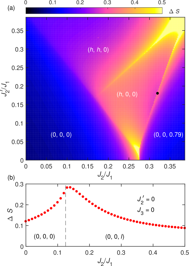
Figure 14: Zero-point spin reduction calculation for CuRh₂O₄. (a) $\Delta S$ as a function of $J_{2}/J_{1}$ and $J_{2}^{\prime}/J_{1}$ with $J_{3}$ varying in order to maintain the propagation vector $\mathbf{k}_{\rm m}=(0,0,0.79)$ spiral phase whenever possible. The black dot corresponds to the parameters obtained for CuRh₂O₄. (b) $\Delta S$ as a function of $J_{2}/J_{1}$ for $J_{2}^{\prime}$ and $J_{3}$ fixed to zero. The vertical dashed line is located at the classical transition ratio ($J_{2}/J_{1}=1/8$) from the Néel state to the incommensurate spiral state.

To evaluate the strength of quantum effects in our diamond-lattice antiferromagnets, we calculate the $1/S$ zero-point reduction on the ordered moment due to quantum fluctuations. In general, the spin reduction $\Delta S_{i}$ is sub-lattice dependent and reads

$$\Delta S_{i}\equiv S-\left<S_{i,\mathbf{R}_{n}}^{z}\right>=\left<a_{i,\mathbf{R}_{n}}^{\dagger}a_{i,\mathbf{R}_{n}}\right>=\frac{1}{\mathcal{N}}\sum\limits_{\mathbf{k}\in\mathrm{B.Z.}}\left<a_{i,\mathbf{q}}^{\dagger}a_{i,\mathbf{q}}\right>,$$ (36)

where $\left<\cdots\right>$ is the thermal average and $\mathcal{N}$ is the number of unit cells in the entire system. Our approach to evaluate $\Delta S_{i}$ uses the transformation matrix $V_{\mathbf{q}}$ obtained from Eq. (26) to transform $a$-bosons into $b$-bosons. As a result,

$$\left<a_{i,\mathbf{q}}^{\dagger}a_{i,\mathbf{q}}\right>= \sum\limits_{j=1}^{2}V^{\dagger}_{j+2,i}V_{i,j+2}$$ (37)

$$+\left[V^{\dagger}_{ji}V_{ij}+V^{\dagger}_{j+2,i}V_{i,j+2}\right]\left<b_{j,\mathbf{q}}^{\dagger}b_{j,\mathbf{q}}\right>,$$

where boson commutation relations are applied. As $\left<b_{i,\mathbf{q}}^{\dagger}b_{i,\mathbf{q}}\right>$ vanishes in the limit $T\!=\!0$, this yields the general formula for the zero-point spin reduction

$$\Delta S_{i} =\frac{1}{\mathcal{N}}\sum\limits_{\mathbf{q}\in\mathrm{B.Z.}}\sum\limits_{j=1}^{2}V^{\dagger}_{j+2,i}V_{i,j+2}$$ (38)

$$=\int_{\mathbf{q}\in\mathrm{B.Z.}}\mathrm{d}^{3}{\bf q}\sum\limits_{j=1}^{2}V^{\dagger}_{j+2,i}V_{i,j+2}\ (\mathcal{N}\rightarrow\infty).$$

When the “two-step diagonalization” is applicable, Eqns. (30, 32) allow us to rewrite the spin reduction in the more traditional form

$$\Delta S_{i}=\frac{1}{\mathcal{N}}\sum\limits_{\mathbf{q}\in\mathrm{B.Z.}}\sum\limits_{j=1}^{2}w^{2}_{ij,\mathbf{q}}v^{2}_{j,\mathbf{q}},$$ (39)

which can be further simplified assuming the two magnetic sites experience the same zero-point reduction,

$$\Delta S =\frac{1}{2}\sum\limits_{j=1}^{2}\int_{\mathbf{q}\in\mathrm{B.Z.}}v^{2}_{j,\mathbf{q}}\mathrm{d}^{3}q\ (\mathcal{N}\rightarrow\infty).$$ (40)

The numerical calculation of Eq. V.3 was implemented in C++ with the help of the adaptive multidimensional integration algorithm.Genz and Malik (1980); Berntsen et al. (1991) Estimated integration errors are generally under 0.5% except for some of critical values of $J^{\prime}s$, e.g., $J_{2}=J_{2}^{\prime}$, for which integration errors are slightly larger. Setting $J_{2}$, $J_{2}^{\prime}$ and $J_{3}$ to zero yields the spin reduction value for the nearest-neighbor 3D diamond-lattice antiferromagnet, $\Delta S_{\Diamond}\!=\!0.11973(1)$, a number significantly smaller than for the nearest-neighbor 2D square-lattice antiferromagnet, $\Delta S_{\square}\!=\!0.19660$. Igarashi (1992)

When competing exchanges relevant for CuRh₂O₄ are included, however, we find that the $1/S$ zero-point reduction dramatically increases for exchange parameters in the vicinity of the mean-field transition lines; see Fig. 14. For the exchange parameters of CuRh₂O₄, we obtain a spin reduction of $\Delta S_{\rm Cu}\!=\!0.330(1)$ and thus predict an ordered moment of $\langle\mu\rangle=g(S-\Delta S_{\rm Cu})\mu_{\rm B}\approx 0.36\mu_{\rm B}$, in qualitative agreement with the strongly reduced moment $\mu_{\rm ord}\!=\!0.56(6)\mu_{\rm B}$ obtained experimentally. We conclude that such a strong reduction of the ordered moment for a 3D magnet originates from competing exchange interactions that place CuRh₂O₄ in the vicinity of a transition line between $\mathbf{k}_{{\rm m},3}=(0,0,\xi)$ and $\mathbf{k}_{{\rm m},2}=(\xi,0,0)$ orders.

VI Conclusion

In conclusion, our detailed experimental and theoretical work identifies the $A$-site spinels CoRh₂O₄ and CuRh₂O₄ as model diamond-lattice antiferromagnets. The cubic compound CoRh₂O₄ is a canonical realization of the nearest-neighbor Heisenberg antiferromagnet on the diamond lattice. Below the Néel temperature $T_{\rm N}\!\approx\!25$ K, the $S=3/2$ magnetic moments order in a bipartite antiferromagnetic structure with a negligible contribution from zero-point fluctuations. Neutron scattering experiments for $T\ll T_{\rm N}$ reveal well-formed spin-wave excitations, successfully described by a single nearest-neighbor magnetic exchange parameter $J_{1}=6.3$ meV. Around and above $T_{\rm N}$, the magnetic excitations rapidly soften and become strongly damped, as expected for a three-dimensional antiferromagnet.

In the tetragonally-distorted $S=1/2$ spinel CuRh₂O₄, the magnetism is much richer and strongly influenced by the competition between nearest-neighbor and further-neighbor exchange interactions. While thermodynamic probes paint a picture remarkably similar to CoRh₂O₄, with a Néel temperature of $T_{\rm N}\approx 24$ K, neutron scattering reveals that the magnetic structure of CuRh₂O₄ is an incommensurate spin helix with a propagation vector $\mathbf{k}_{\rm m}=(0,0,0.79)$ and strong quantum reduction of the ordered magnetic moments to $\approx 50$% of their classical value. Comparison between inelastic neutron scattering results and spin-wave theory provides a quantitative understanding of the underlying microscopic mechanism responsible for this unexpected ground state. Due to the tetragonal lattice symmetry, the degeneracy between second-neighbor exchanges ($J_{2}$ and $J_{2}^{\prime}$) is lifted when compared to the cubic case. Our mean-field calculation shows that the competition of these exchanges with first- ($J_{1}$) and third-neighbor ($J_{3}$) interactions stabilizes the incommensurate spin helix observed experimentally. Remarkably, we find that CuRh₂O₄ lies close to a transition between two distinct magnetically ordered ground-states. Using $1/S$-corrections to the ordered moment, we find that zero-point fluctuations are enhanced for the exchange parameters of CuRh₂O₄, which explains the strong moment reduction observed experimentally.

Overall, our results add two model magnets to the expanding family of diamond-lattice antiferromagnets and further demonstrate the importance of competing exchange interactions and possible enhancement of quantum effects in such systems. We expect our results on CuRh₂O₄ to guide future studies to elucidate the spin-liquid phenomenology recently uncovered in the isostructural compound NiRh₂O₄, Chamorro and McQueen (2017) and more generally to contribute to the search for the predicted topological paramagnetism in $S=1$ diamond-lattice antiferromagnets. Wang et al. (2015) On the methodological side, our work demonstrates that combining state-of-the-art neutron scattering experiments with mean-field and spin-wave theory modeling allows to extract definitive microscopic information from polycrystalline samples alone, even when magnetic correlations are three-dimensional. This is important to accelerate the search for exotic quantum states in real systems through the screening of many related materials, an endeavor that would be too costly, difficult or slow to undertake on single-crystalline samples.

Appendix A Conventional and primitive cells

In the case of CuRh₂O₄, the primitive $(\bm{a}_{\rm p},\bm{b}_{\rm p},\bm{c}_{\rm p})$ and conventional $(\bm{a},\bm{b},\bm{c})$ crystallographic unit cells are related by:

$$\left(\begin{array}[]{c}\bm{a}_{\rm p}\\ \bm{b}_{\rm p}\\ \bm{c}_{\rm p}\end{array}\right)\!=\!\frac{1}{2}\left(\begin{array}[]{rrr}1&1&-1\\ -1&1&1\\ 1&-1&1\end{array}\right)\left(\begin{array}[]{c}\bm{a}\\ \bm{b}\\ \bm{c}\end{array}\right).$$ (41)

This yields the following relations between the Miller indices $(h,k,l)$ and atomic fractional coordinates $(x,y,z)$ for the two unit cells,

$$\left(x_{\mathrm{p}},y_{\mathrm{p}},z_{\mathrm{p}}\right) = \left(x+y,y+z,x+z\right)$$ (42)

$$\left(2h_{\mathrm{p}},2k_{\mathrm{p}},2l_{\mathrm{p}}\right) = \left(h+k+l,-h+k+l,h-k+l\right),$$

such that the primitive unit cell of CuRh₂O₄ contains two Cu atoms, at fractional coordinates $\mathbf{r}_{1}=(0,0,0)$ and $\mathbf{r}_{2}=(\frac{1}{2},\frac{3}{4},\frac{1}{4})$.

Appendix B Classical ground state energy minimization

In this appendix, we provide general expressions for the classical ground-state energy per spin and magnetic structure for different phases of our mean-field phase diagram. Working in the primitive unit cell, the magnetic structure is fully defined from the knowledge of $\varphi$, the angle between two spins in one primitive cell, and $\gamma$ the pitch angle between neighbor cells that enters the propagation vector $\mathbf{k}_{\rm m}$.

In the case of the $\mathbf{k}_{{\rm m},3}=(0,0,\gamma/\pi)$ phase, the classical energy per spin reads

$$\mathcal{H}_{0}=S^{2}\left\{\right. \left.J_{1}\left[\cos\varphi+\cos(\varphi-\gamma)\right]+4J_{2}\cos\gamma+2J_{2}^{\prime}\right.$$

$$+ \left.J_{3}\left[\cos(2\gamma-\varphi)+\cos(\gamma+\varphi)\right]\right\}.$$

The local minimum conditions, ${\partial\mathcal{H}_{0}}/{\partial\varphi}=0$ and ${\partial\mathcal{H}_{0}}/{\partial\gamma}=0$ and the intuitive assumption of a uniform angle between spins along $\bm{c}$, $\cos\gamma=\cos 2\varphi$, lead to

$$\cos\varphi = -\frac{1}{6J_{3}}\left(\sqrt{4J_{2}^{2}-3J_{1}J_{3}+9J_{3}^{2}}-2J_{2}\right)\ (J_{3}\neq 0),$$

$$\cos\varphi = -\frac{J_{1}}{8J_{2}}\ (J_{3}=0).$$

Similarly, the expression for the classical energy per spin in the $\mathbf{k}_{{\rm m},2}=(\gamma/\pi,0,0)$ phase is

$$\mathcal{H}_{0}=S^{2}\left\{\right. (J_{1}+J_{3})\left[2\cos\varphi+\cos(\varphi-2\gamma)+\cos(\varphi+2\gamma)\right]$$

$$+ \left.8J_{2}\cos\gamma+2J_{2}^{\prime}\cos 2\gamma\right\}.$$

This is not easy to solve directly without any extra information. However, with the help of mean-field calculations, we find $\varphi=\pi$, which yields

$$\cos\gamma=\frac{J_{1}+J_{3}-4J_{2}}{4J_{2}^{\prime}}.$$

Finally, for the $\mathbf{k}_{{\rm m},1}=(\gamma/\pi,\gamma/\pi,0)$ phase, the expression for the classical energy per spin is

$$\mathcal{H}_{0}=S^{2}\left\{\right. \left.(J_{1}+J_{3})\left[\cos\varphi+\cos(\varphi-\gamma)\right]\right.$$

$$+ \left.2J_{2}\cos\gamma+2J_{2}^{\prime}\cos\gamma+2J_{2}\right\}.$$

It is straightforward to solve the local minimum conditions without making any assumptions, which yields

$$\cos\varphi=-\frac{J_{1}+J_{3}}{4(J_{2}+J_{2}^{\prime})};$$

$$\cos\gamma=-1+\frac{(J_{1}+J_{3})^{2}}{8(J_{2}+J_{2}^{\prime})^{2}}.$$

References

- Affleck (1989) I. Affleck, J. Phys. Condens. Matter 1, 3047 (1989).
- Mikeska and Kolezhuk (2004) H.-J. Mikeska and A. K. Kolezhuk, in Quantum magnetism (Springer, 2004) pp. 1–83.
- Lake et al. (2005) B. Lake, D. A. Tennant, C. D. Frost, and S. E. Nagler, Nat. Mat. 4, 329 (2005).
- Coldea et al. (2010) R. Coldea, D. Tennant, E. Wheeler, E. Wawrzynska, D. Prabhakaran, M. Telling, K. Habicht, P. Smeibidl, and K. Kiefer, Science 327, 177 (2010).
- Ramirez (1994) A. Ramirez, Annu. Rev. Mater. Sci. 24, 453 (1994).
- Lee (2008) P. A. Lee, Science 321, 1306 (2008).
- Han et al. (2012) T.-H. Han, J. S. Helton, S. Chu, D. G. Nocera, J. A. Rodriguez-Rivera, C. Broholm, and Y. S. Lee, Nature 492, 406 (2012).
- Savary and Balents (2016) L. Savary and L. Balents, Rep. Prog. Phys. 80, 016502 (2016).
- Jackeli and Khaliullin (2009) G. Jackeli and G. Khaliullin, Phys. Rev. Lett. 102, 017205 (2009).
- Banerjee et al. (2017) A. Banerjee, J. Yan, J. Knolle, C. A. Bridges, M. B. Stone, M. D. Lumsden, D. G. Mandrus, D. A. Tennant, R. Moessner, and S. E. Nagler, Science 356, 1055 (2017).
- Chisnell et al. (2015) R. Chisnell, J. S. Helton, D. E. Freedman, D. K. Singh, R. I. Bewley, D. G. Nocera, and Y. S. Lee, Phys. Rev. Lett. 115, 147201 (2015).
- Hirschberger et al. (2015) M. Hirschberger, R. Chisnell, Y. S. Lee, and N. P. Ong, Phys. Rev. Lett. 115, 106603 (2015).
- Chernyshev and Maksimov (2016) A. L. Chernyshev and P. A. Maksimov, Phys. Rev. Lett. 117, 187203 (2016).
- Bramwell and Gingras (2001) S. T. Bramwell and M. J. Gingras, Science 294, 1495 (2001).
- Gardner et al. (2010) J. S. Gardner, M. J. Gingras, and J. E. Greedan, Rev. Mod. Phys. 82, 53 (2010).
- Fennell et al. (2009) T. Fennell, P. Deen, A. Wildes, K. Schmalzl, D. Prabhakaran, A. Boothroyd, R. Aldus, D. McMorrow, and S. Bramwell, Science 326, 415 (2009).
- Ross et al. (2011) K. A. Ross, L. Savary, B. D. Gaulin, and L. Balents, Phys. Rev. X 1, 021002 (2011).
- Krimmel et al. (2006) A. Krimmel, M. Mücksch, V. Tsurkan, M. M. Koza, H. Mutka, C. Ritter, D. V. Sheptyakov, S. Horn, and A. Loidl, Phys. Rev. B 73, 014413 (2006).
- Gao et al. (2016) S. Gao, O. Zaharko, V. Tsurkan, Y. Su, J. S. White, G. S. Tucker, B. Roessli, F. Bourdarot, R. Sibille, D. Chernyshov, T. Fennell, A. Loidl, and C. Ruegg, Nat. Phys. 13, 157–161 (2016).
- Bergman et al. (2007) D. Bergman, J. Alicea, E. Gull, S. Trebst, and L. Balents, Nat. Phys. 3, 487 (2007).
- Bernier et al. (2008) J.-S. Bernier, M. J. Lawler, and Y. B. Kim, Phys. Rev. Lett. 101, 047201 (2008).
- Fritsch et al. (2004) V. Fritsch, J. Hemberger, N. Büttgen, E.-W. Scheidt, H.-A. Krug von Nidda, A. Loidl, and V. Tsurkan, Phys. Rev. Lett. 92, 116401 (2004).
- Krimmel et al. (2005) A. Krimmel, M. Mücksch, V. Tsurkan, M. M. Koza, H. Mutka, and A. Loidl, Phys. Rev. Lett. 94, 237402 (2005).
- Laurita et al. (2015) N. J. Laurita, J. Deisenhofer, L. Pan, C. M. Morris, M. Schmidt, M. Johnsson, V. Tsurkan, A. Loidl, and N. P. Armitage, Phys. Rev. Lett. 114, 207201 (2015).
- Mittelstädt et al. (2015) L. Mittelstädt, M. Schmidt, Z. Wang, F. Mayr, V. Tsurkan, P. Lunkenheimer, D. Ish, L. Balents, J. Deisenhofer, and A. Loidl, Phys. Rev. B 91, 125112 (2015).
- Plumb et al. (2016) K. W. Plumb, J. R. Morey, J. A. Rodriguez-Rivera, H. Wu, A. A. Podlesnyak, T. M. McQueen, and C. L. Broholm, Phys. Rev. X 6, 041055 (2016).
- Biffin et al. (2017) A. Biffin, C. Rüegg, J. Embs, T. Guidi, D. Cheptiakov, A. Loidl, V. Tsurkan, and R. Coldea, Phys. Rev. Lett. 118, 067205 (2017).
- Chen et al. (2009a) G. Chen, L. Balents, and A. P. Schnyder, Phys. Rev. Lett. 102, 096406 (2009a).
- Chen et al. (2009b) G. Chen, A. P. Schnyder, and L. Balents, Phys. Rev. B 80, 224409 (2009b).
- Suzuki et al. (2007) T. Suzuki, H. Nagai, M. Nohara, and H. Takagi, J. Phys. Condens. Matter 19, 145265 (2007).
- MacDougall et al. (2011) G. J. MacDougall, D. Gout, J. L. Zarestky, G. Ehlers, A. Podlesnyak, M. A. McGuire, D. Mandrus, and S. E. Nagler, Proc. Natl. Acad. Sci. USA 108, 15693 (2011).
- Zaharko et al. (2014) O. Zaharko, S. Tóth, O. Sendetskyi, A. Cervellino, A. Wolter-Giraud, T. Dey, A. Maljuk, and V. Tsurkan, Phys. Rev. B 90, 134416 (2014).
- MacDougall et al. (2016) G. J. MacDougall, A. A. Aczel, Y. Su, W. Schweika, E. Faulhaber, A. Schneidewind, A. D. Christianson, J. L. Zarestky, H. D. Zhou, D. Mandrus, and S. E. Nagler, Phys. Rev. B 94, 184422 (2016).
- Wang et al. (2015) C. Wang, A. Nahum, and T. Senthil, Phys. Rev. B 91, 195131 (2015).
- Haldane (1983) F. D. M. Haldane, Phys. Rev. Lett. 50, 1153 (1983).
- Affleck et al. (1987) I. Affleck, T. Kennedy, E. H. Lieb, and H. Tasaki, Phys. Rev. Lett. 59, 799 (1987).
- Chamorro and McQueen (2017) J. R. Chamorro and T. M. McQueen, arXiv preprint arXiv:1701.06674 (2017).
- Chen (2017) G. Chen, arXiv preprint arXiv:1701.05634 (2017).
- Rodriguez-Carvajal (1993) J. Rodriguez-Carvajal, Physica B 192, 55 (1993).
- Bain and Berry (2008) G. A. Bain and J. F. Berry, Journal of Chemical Education 85, 532 (2008).
- Garlea et al. (2010) V. O. Garlea, B. C. Chakoumakos, S. A. Moore, G. B. Taylor, T. Chae, R. G. Maples, R. A. Riedel, G. W. Lynn, and D. L. Selby, Applied Physics A 99, 531 (2010).
- Granroth et al. (2010) G. E. Granroth, A. I. Kolesnikov, T. E. Sherline, J. P. Clancy, K. A. Ross, J. P. C. Ruff, B. D. Gaulin, and S. E. Nagler, J. Phys.: Conf. Series 251, 012058 (2010).
- Stone et al. (2014) M. B. Stone, J. L. Niedziela, D. L. Abernathy, L. DeBeer-Schmitt, G. Ehlers, O. Garlea, G. E. Granroth, M. Graves-Brook, A. I. Kolesnikov, A. Podlesnyak, and B. Winn, Rev. Sci. Instrum. 85, 045113 (2014).
- Petit, S (2011) Petit, S, JDN 12, 105 (2011).
- Toth and Lake (2015) S. Toth and B. Lake, J. Phys. Condens. Matter 27, 166002 (2015).
- Blasse (1963) G. Blasse, Philips Res. Repts 18, 383 (1963).
- Bertaut et al. (1959) F. Bertaut, F. Forrat, and J. Dulac, Comptes Rendus Hebdomadaires des Seances de l’Academie des Sciences 249, 726 (1959).
- Cascales and Rasines (1984) C. Cascales and I. Rasines, Materials Chemistry And Physics 10, 199 (1984).
- Brown (1981) I. D. Brown, The bond-valence method: an empirical approach to chemical structure and bonding (Academic Press, New York, 1981) pp. 1–30.
- Blasse and Schipper (1963) G. Blasse and D. J. Schipper, Phys. Lett. 5, 300 (1963).
- Fiorani and Viticoli (1979) D. Fiorani and S. Viticoli, Solid State Commun. 29, 239 (1979).
- Campbell et al. (2006) B. J. Campbell, H. T. Stokes, D. E. Tanner, and D. M. Hatch, J. Appl. Crystallogr. 39, 607 (2006).
- Miller and Love (1967) S. C. Miller and W. F. Love, Tables of Irreducible Representations of Space Groups and Co-representations of Magnetic Space Groups (Pruett Press, Boulder, Colorado, 1967).
- Rønnow et al. (1999) H. M. Rønnow, D. F. McMorrow, and A. Harrison, Phys. Rev. Lett. 82, 3152 (1999).
- Khanolkar (1961) D. Khanolkar, Current Science 30, 52 (1961).
- Ismunandar et al. (1999) Ismunandar, B. J. Kennedy, and B. A. Hunter, Mat. Res. Bull. 34, 135 (1999).
- Dollase and O’Neill (1997) W. Dollase and H. S. C. O’Neill, Acta Crystallogr. Sec. C 53, 657 (1997).
- Endoh et al. (1999) R. Endoh, O. Fujishima, T. Atake, N. Matsumoto, M. Hayashi, and S. Nagata, J. Phys. Chem. Solids 60, 457 (1999).
- Bertaut (1962) E. F. Bertaut, Journal of Applied Physics 33, 1138 (1962).
- Chapon (2009) L. C. Chapon, Phys. Rev. B 80, 172405 (2009).
- Reimers et al. (1991) J. N. Reimers, A. J. Berlinsky, and A.-C. Shi, Phys. Rev. B 43, 865 (1991).
- Chernyshev and Zhitomirsky (2015) A. L. Chernyshev and M. E. Zhitomirsky, Phys. Rev. B 92, 144415 (2015).
- Genz and Malik (1980) A. C. Genz and A. Malik, J. Comput. Phys. and Appl. Maths. 6, 295 (1980).
- Berntsen et al. (1991) J. Berntsen, T. O. Espelid, and A. Genz, ACM Transactions on Mathematical Software (TOMS) 17, 437 (1991).
- Igarashi (1992) J.-I. Igarashi, Phys. Rev. B 46, 10763 (1992).