Deadline-Aware Multipath Communication:
An Optimization Problem

Abstract

Multipath communication not only allows improved throughput but can also be used to leverage different path characteristics to best fulfill each application’s objective. In particular, certain delay-sensitive applications, such as real-time voice and video communications, can usually withstand packet loss and aim to maximize throughput while keeping latency at a reasonable level. In such a context, one hard problem is to determine along which path the data should be transmitted or retransmitted. In this paper, we formulate this problem as a linear optimization, show bounds on the performance that can be obtained in a multipath paradigm, and show that path diversity is a strong asset for improving network performance. We also discuss how these theoretical limits can be approached in practice and present simulation results.

I Introduction

Looking back in history, many computer systems were initially designed to use only a single resource of each type (e.g., processor, memory, display) at once. Over time, to increase the performance of these systems, we have seen the development of better components (in terms of speed, capacity, or size) and more efficient algorithms; but these options are limited by the laws of physics, the ingenuity of researchers, and the nature of the problem. Parallelism emerged as the other options faced barriers (as illustrated by the development of multicore processors, for example). Oddly, the idea of applying parallelism to network paths (i.e., using multipath protocols) has only started to get traction recently, with Multipath TCP [1] in particular.

There is an ongoing effort to develop new network protocols and improve existing ones, but even with an optimal communication strategy, performance depends on the underlying medium of data transfer. Among the different physical means of carrying data that we know of (e.g., optical fiber, electromagnetic radiation, or a pair of conductors), there is no panacea. Fiber unquestionably allows greater throughput than copper wires, for example, but microwaves offer an important advantage for mobility and can significantly cut latency. In fact, the speed of microwaves on the surface of the earth is close to the speed of light in vacuum, whereas fiber only achieves roughly $2/3$ of that speed [2] (even when assuming a straight line between source and destination). However, these benefits come at a cost, namely higher loss rates (which depend on distance and other environmental conditions) and lower bandwidth.

In a near future, we might witness the appearance of even more heteroclite networks with projects such as Facebook’s Aquila [3] (based on solar-powered drones), Google’s Project Loon [4] (based on high-altitude balloons), or SpaceX’s project to provide Internet with low-orbit satellites [5]. Furthermore, future Internet architectures could explicitly provide multiple paths to end hosts [6, 7, 8, 9, 10] and these paths might also exhibit very diverse properties. As sending multiple packets over a network in which multiple paths are available is a parallelizable task by nature, we claim that it is possible to take advantage of this situation to accomplish a broad set of application-level objectives, such as latency-related objectives. Unfortunately, as of today, few protocols make use of multiple network paths simultaneously.

Because most applications are sensitive to latency to some extent, we distinguish between two main classes of applications. The first class concerns applications that need a reliable transport protocol—typically TCP or a variant thereof (possibly with multipath functionalities and/or optimized for latency, see Section III). This class encompasses file transfers, web browsing, and more. For these applications latency might be an important concern, but reliability is the critical requirement. The second class relates to real-time applications, which typically do not use a reliable protocol. The reasons for not using a fully reliable service are the following. By definition, reliable protocols never discard any packet before the sender receives an acknowledgment—even if the packet in question is obsolete from the application’s perspective. Moreover, ordered byte-stream protocols suffer from the head-of-line blocking problem, and cannot give any guarantee regarding the time at which a packet will be delivered. As a consequence, it is hard to specify strict latency-related objectives when a reliable protocol such as TCP is considered; hence real-time applications typically use UDP instead. The problem when using UDP is that transport-layer duties (e.g., retransmissions, congestion control) are delegated to the application layer, thus every application must re-implement the same mechanisms. Furthermore, as of today, multipath functionalities are not natively available to the developers of such applications.

In this paper, we focus on real-time applications and consider one particular communication scenario in which the objective is to deliver as much data as possible before a deadline across multiple end-to-end paths. After the deadline, the data can be discarded (i.e., the communication is not fully reliable, but gives latency guarantees). There is a plethora of applications that would benefit from a deadline-aware protocol: voice communication, videoconferencing, live video streaming, online gaming, high-frequency trading, and more. The lifetime of a packet for these various applications could range from a few milliseconds to several seconds. Therefore, it is crucial that practical techniques as well as theoretical foundations be developed for partially reliable multipath communications.

Using multiple paths simultaneously implies that the sender might have to make hard decisions regarding packet-to-path assignments when the available paths have different properties. It may not be obvious that path diversity can help improve network performance. Is it preferable to have identical paths (in which case the packet assignment problem becomes irrelevant) or diverse ones? Also, if diverse paths are available, is the optimal strategy to always use only one of these paths (the most appropriate one from the application perspective)? Intuitively, diversity allows each path to specialize in a different task. High-bandwidth paths can carry the initial data transmission, and low-latency low-loss paths present advantages for retransmissions and control data (e.g., acknowledgments). We provide a model that allows determining the potential benefits of any given set of paths and we show in our evaluation that having complementary paths is beneficial in a deadline-based communication context to.

II Problem Description

One typical situation in which two paths are available is when a smartphone is connected to both a WiFi access point and a cellular network. This can lead to very different outcomes depending on which path is selected. Bandwidth depends on which generation of the technology in question is used (e.g., 3G, 4G, 802.11a, b, g). Losses depend on congestion, environmental conditions, and more. Finally, delay is in part influenced by the signal quality as retransmissions can be performed at the link layer.

Figure 1 represents a simple instance of the multipath-related problem that we study in this paper. There are two paths with contrasting characteristics and the source generates a constant flow of data that must be delivered, at the latest, after one second. As the one-way delay of the high-bandwidth path is 600 ms, it will take 800 ms in total for an acknowledgment to come back along the low-latency path (assumption motivated in Section VIII-C), which leaves enough time to (potentially) retransmit the data along the low-latency path. Clearly, if all the generated data is initially sent along the high-bandwidth path and retransmitted along the low-bandwidth path, we can expect 100% of the packets to reach their destination in time. This would not be possible by using only one of the two paths.

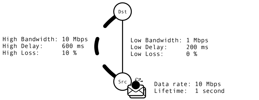
Figure 1: Deadline-based multipath communication scenario.

This instance of the problem is trivial, i.e., an optimal solution can be found intuitively. However, the problem becomes hard when more paths are considered or when the metrics do not naturally produce such a straightforward solution. The question we will try to answer is the following: how can the generalization of the problem (to an arbitrary number of paths with any characteristics) be solved?

III Related Work

Multipath TCP (MPTCP) [1] is the de-facto standard multipath transport protocol. It received much attention when it was adopted by Apple for its personal-assistant software, Siri. As MPTCP is based on TCP, it suffers from the head-of-line blocking problem and other issues we mention in this paper; hence it is not particularly adapted to latency-sensitive applications. D²TCP [13], on the other hand, is an example of deadline-based protocol, but it was specially designed for data centers, not for general-purpose settings over inter-domain networks. Moreover, D²TCP is not a multipath protocol. The partial-reliability extension of the Stream Control Transmission Protocol (PR-SCTP) [14] offers the primitive that we examine in this paper, i.e., a possibility to define a lifetime parameter. Although PR-SCTP offers multihoming capabilities, additional IP addresses are used as a backup in case of failure, so PR-SCTP is not a fully multipath protocol and does not address the problem that we describe in this paper [15].

Diverse techniques have been used in recent work to analyze and leverage the benefits of multipath communication. Liu et al. [16] used linear programming to evaluate multipath routing from a traffic engineering perspective. They presented the somewhat counterintuitive result that multipath routing offers limited gain compared to single-path routing in terms of load balancing (under specific traffic conditions and for certain types of network topology). However, their work—contrarily to ours—focuses on the distribution of traffic over the network and does not take deadlines into account. Soldati et al. [17] addressed the problem of scheduling and routing packets with deadlines in a network whose topology is known (represented as a directed acyclic graph), whereas we only assume end-to-end paths. The work of Wu et al. [18] might be the closest to ours, but with one important difference: they propose a method to assign entire flows (with different data rates and a deadline) to specific paths, which does not allow using an optimal retransmission strategy. Our work falls into another category: packet-based traffic splitting [19, 20]. The novelty of our approach is that we leverage linear programming to find an optimal solution to a packet-to-path assignment problem, from the end-host’s perspective, while taking cost, retransmissions, and strict latency constraints into account. Also, we show how to integrate random delays into our model.

IV Background

In this section, we present our system assumptions and a few definitions. We consider a network setup with a set of paths—each bearing possibly different characteristics—between one source and one destination. The source generates a flow of data at a constant bit rate and can split this data and select the paths along which each part will be transmitted. In practice, the different paths could, for example, correspond to different network interfaces (which is the typical configuration that MPTCP relies on [1]). Each bit must be delivered before a specific point in time that we call the deadline. To avoid any confusion, we distinguish between a deadline, which must be interpreted as an absolute time (e.g., 1:23:45 pm GMT), and the data’s lifetime, which must be interpreted as a relative time (e.g., 500 ms). We consider the lifetime to be the same for all the data, whereas the deadline depends on the lifetime and the moment when the data was generated.

In addition to the standard bandwidth, delay, and loss characteristics of a network path, we consider the cost of transmitting one bit along each path and set a user-selectable upper bound on the total usage cost per unit time. A cost can be seen, intuitively, as an amount of money that the user must pay to utilize the path, but it can also be used to model other consequences of using a path, such as power consumption. A system is hence characterized by the parameters presented in Table I.

TABLE I: Network Characteristics

	Description
$n$	number of independent paths
$\lambda$	data rate generated by the application
$\delta$	data lifetime
$\mu$	upper bound on total cost per second
$b_{i}$	bandwidth of path $i$
$d_{i}$	one-way delay of path $i$
$\tau_{i}$	probability of bit erasure on path $i$
$c_{i}$	cost of sending one bit along path $i$

Moreover, we define $d_{\textit{min}}$ (seconds) as the shortest delay of all paths, i.e.,

$$d_{\textit{min}}=\min_{i}d_{i}.$$ (1)

Losses are modeled by a binary erasure channel. This choice is motivated by the fact that we operate at the transport layer where checksums are usually employed. When the verification of a checksum fails, the packet is dropped without notifying the receiver, which is equivalent to a bit erasure. However, we do not consider a specific packet size; instead, we use general characteristics such as the average loss rate.

V Model

We now propose a model whose purpose is to capture the optimal multipath sending strategy for the scenario presented above. This model can be used to provide theoretical upper bounds on the performance of an ideal protocol under specific conditions, but it can also be used to design an actual protocol (if combined with different techniques and heuristics, as described in the following sections).

The problem under study is to determine what ratio of the traffic generated by the application should be transmitted/retransmitted along each path, so that the maximal amount of data arrives in time at the destination. Because we take latency into account, the paths for initial transmission and for retransmission must be considered jointly. We call this pair of transmission/retransmission paths a path combination. The objective is to find optimal values for the variables contained in the following matrix:

$x$: matrix of size $n$-by-$n$, where $x_{i,j}$ is the proportion of data to send along path $i$ and then, if needed, along path $j$ (for a retransmission).

We then rearrange these variables into a vector, so that the problem can be solved with a standard form of linear programming:

$x^{\prime}$: vector of size $n^{2}$, given by the vectorization of $x$.

Only one retransmission is considered here in order to avoid a cumbersome notation, but this model can clearly be adapted to an arbitrary number of retransmissions, although the complexity of solving the problem will naturally increase with the number of retransmissions considered, as discussed in Section VIII-B. We envision that, in most real cases, the problem would be solved for a maximum of 2–3 retransmissions, for two reasons. First, unless the loss rate is particularly high on all paths, having to send the same data 4 times or more is a very rare event. Second, the time it takes to perform many retransmissions is likely to exceed the lifetime.

V-A Network metrics

We define several metrics to measure the outcomes of choosing certain values of $x$ for a given network. This will help to define conditions and objectives in the linear program. The metrics notation that we use is summarized in Table II.

TABLE II: Network Metrics

	Description
$S_{i}$	bit rate sent along path $i$
$G$	goodput, i.e., useful received data rate
$Q$	communication quality (ratio of $G$ to $\lambda$)
$C$	total cost per second (sum of all paths)

First, the amount of data sent on a certain path is obtained by considering both the data that is sent for the first time on that path (whatever the path along which the same data might then be retransmitted) and the data that is retransmitted on that path (which depends on the reliability of the initial path). Therefore, we have

$$S_{i}=\sum_{j=0}^{n-1}x_{i,j}\cdot\lambda+\sum_{j=0}^{n-1}x_{j,i}\cdot\lambda\cdot\tau_{j}.$$ (2)

This must be bounded by the available bandwidth on the corresponding path:

$$S_{i}\leq b_{i}\quad\forall~{}i\in\{0,1,\dots,n-1\}.$$ (3)

Because we assume that the delay is fixed (relaxed in Section VI) and that an acknowledgment always comes back on the path with the shortest delay (discussed in Section VIII-C), when data is sent along path $i$, the sender sets a retransmission timeout to

$$t_{i}=d_{i}+d_{\text{min}}.$$ (4)

We define goodput as the amount of application data that arrives at the destination before the deadline each second. Again, we must consider both data that arrives on the first attempt, and retransmitted data. As a result, the goodput is defined as

$$G =\sum_{i:d_{i}\leq\delta}\sum_{j=0}^{n-1}x_{i,j}\cdot(1-\tau_{i})\cdot\lambda$$ (5)

$$+\sum_{i,j:d_{i}+d_{\textit{min}}+d_{j}\leq\delta}x_{i,j}\cdot\tau_{i}\cdot(1-\tau_{j})\cdot\lambda.$$

Goodput depends on how much data the application generates (i.e., $\lambda$), but we are interested in determining the proportion of $\lambda$ that a given network can handle with an optimal strategy. Therefore, we define our main metric, which we call communication quality, as

$$Q=\frac{G}{\lambda}.$$ (6)

It follows that $0\leq Q\leq 1$ (a quality of 1 meaning that all the data arrives at the destination before the deadline).

The total cost $C$ is defined as the sum of all per-path costs per second. We require the total cost to be bounded by a constant $\mu$. This allows us to maximize communication quality while keeping cost to a reasonable level, but $\mu$ can be set arbitrarily high if the cost does not have to be limited. Therefore, the total cost is defined and bounded as follows:

$$C=\sum_{i=0}^{n-1}c_{i}\cdot S_{i}\leq\mu.$$ (7)

Finally, the sum of all coefficients in $x$ must equal 1. In other words, all the bits generated by the application must be sent over the network along some combination of paths. On one hand, we do not want to send more data than what the application generates. On the other hand, the reason why we never send less data is that we can achieve a more fine-grained decision of whether data should be dropped through an additional dedicated path (the blackhole path, presented in Section V-C). Therefore, we have

$$\sum_{i=0}^{n-1}\sum_{j=0}^{n-1}x_{i,j}=1,$$ (8)

$$x_{i,j}\geq 0\quad\forall~{}i,j\in\{0,1,\dots,n-1\}.$$ (9)

V-B Linear Programming

We formulate our problem as a standard linear optimization:

$$\begin{array}[]{ll}\text{maximize}&p^{\text{T}}x^{\prime},\\ \text{subject to}&Ax^{\prime}\leq q,\\ &Bx^{\prime}=1,\\ \text{and}&x^{\prime}\geq 0.\end{array}$$ (10)

The objective is to maximize the communication quality $Q$, which is captured by $p$ and follows from Equations 5 and 6. Each element of $p$ corresponds to a different path combination and represents the proportion of data that can be delivered in time by using that particular combination:

$$p^{\text{T}}=(p_{0},p_{1},\dots,p_{n^{2}-1}),$$ (11)

$$p_{l}=\left\{\begin{array}[]{ll}1-(\tau_{i}\cdot\tau_{j})&\text{if }d_{i}+d_{\textit{min}}+d_{j}\leq\delta,\\ 1-\tau_{i}&\text{if }d_{i}+d_{\textit{min}}+d_{j}>\delta\text{ and }d_{i}\leq\delta,\\ 0&\text{otherwise}.\end{array}\right.$$ (12)

In the above equation, $i$ and $j$ are defined as follows:

$$\begin{gathered}i=l\bmod n,\\ j=\left\lfloor\frac{l}{n}\right\rfloor.\end{gathered}$$ (13)

We define $i$ and $j$ from $l$ to convert indexes back to the original (non-vectorized) notation used in $x$.

Bandwidth constraints, as presented in Equations 2 and 3, are defined by coefficients in $A$, from $A_{0,0}$ to $A_{n-1,n^{2}-1}$:

$$A=\begin{pmatrix}A_{0,0}&A_{0,1}&\cdots&A_{0,n^{2}-1}\\ A_{1,0}&A_{1,1}&\cdots&A_{1,n^{2}-1}\\ \vdots&\vdots&\ddots&\vdots\\ A_{n-1,0}&A_{n-1,1}&\cdots&A_{n-1,n^{2}-1}\\ r_{0}&r_{1}&\cdots&r_{n^{2}-1}\\ \end{pmatrix},$$ (14)

$$A_{k,l}=\left\{\begin{array}[]{ll}\lambda+\lambda\cdot\tau_{i}&\text{if }i=j=k,\\ \lambda\cdot\tau_{i}&\text{if }i\neq k\text{, }j=k,\\ \lambda&\text{if }j\neq k\text{, }i=k,\\ 0&\text{otherwise.}\\ \end{array}\right.$$ (15)

The cost constraint (Equation 7) is defined with the remaining coefficients in $A$, from $r_{0}$ to $r_{n^{2}-1}$:

$$r_{l}=(\lambda\cdot c_{i})+(\lambda\cdot\tau_{i}\cdot c_{j}),$$ (16)

where $i$ and $j$ are defined as in Equation 13.

The vector $q$ allows us to specify the upper bounds on bandwidth and cost:

$$q=\begin{pmatrix}b_{0}\\ b_{1}\\ \vdots\\ b_{n-1}\\ \mu\\ \end{pmatrix}.$$ (17)

Finally, $B$ is used to enforce the constraint of Equation 8, i.e., to ensure that all the generated traffic is assigned to some path combination:

$$B=\begin{pmatrix}1&1&\cdots&1\end{pmatrix}.$$ (18)

V-C Blackhole Path

When the bitrate $\lambda$ exceeds the network’s capacity, part of the data must be dropped. The model above does not allow that situation to be represented directly. If the sign in Equation 8 was changed to $\leq$, then the total amount of data (sent on all paths combined) could be less than $\lambda$. However, the optimal solution might consist in sending data but not retransmitting it, which the above method does not allow. Instead, one solution is to dedicate a virtual path to the function of discarding data. We refer to it as the “blackhole path” and it has the following characteristics:

$$b_{0}=\lambda,\quad d_{0}=\infty,\quad\tau_{0}=1,\quad c_{0}=0.$$ (19)

Sending data along this path is equivalent to discarding the data, and this path can be selected at any stage of (re)transmission.

VI Extensions

Our model can be extended and transformed in several ways to specify different objectives or consider more complex network characteristics.

VI-A Minimizing Cost

Instead of maximizing communication quality for a given maximum cost, it is possible to solve the opposite problem, i.e., minimize cost for a given minimum quality:

$$\begin{array}[]{ll}\text{minimize}&p^{\text{T}}x^{\prime},\\ \text{subject to}&Ax^{\prime}\leq q,\\ &Bx^{\prime}=1,\\ \text{and}&x^{\prime}\geq 0.\end{array}$$ (20)

The objective, represented by $p_{l}$, must be redefined as follows:

$$p_{l}=(\lambda\cdot c_{i})+(\lambda\cdot\tau_{i}\cdot c_{j}).$$ (21)

The bandwidth-related constraints (defined in $A$) and $B$ remain the same, but the cost constraint (defined in $r_{k}$ and $q$) becomes a quality constraint:

$$r_{l}=\left\{\begin{array}[]{ll}\tau_{i}\cdot\tau_{j}-1&\text{if }d_{i}+d_{\textit{min}}+d_{j}\leq\delta,\\ \tau_{i}-1&\text{if }d_{i}+d_{\textit{min}}+d_{j}>\delta\text{ and }d_{i}\leq\delta,\\ 0&\text{otherwise},\end{array}\right.$$ (22)

where $i$ and $j$ are defined as in Equation 13, and

$$q=\begin{pmatrix}b_{0}\\ b_{1}\\ \vdots\\ b_{n-1}\\ \mu\end{pmatrix},$$ (23)

where $\mu$ is, in this case, the lower bound on quality (instead of being an upper bound on cost).

VI-B Random delays

Up to this point, we assumed that the delay observed on each path was constant. Let’s now consider instead that delays follow probability distributions. We denote by $d_{i}$ the random variable representing the delay of a transmission on path $i$, which follows a probability distribution $D_{i}$, i.e.,

$$d_{i}\sim D_{i}.$$ (24)

One problem that arises in this situation is that the sender must determine an additional parameter for each path combination, namely the waiting time between the moment a packet is sent and the moment when it is possibly retransmitted. We call this the retransmission timeout and denote it $t_{i,j}$.

The receiver must also choose a path (with delay $d_{\textit{min}}$) to send acknowledgements back. We define this path to be the one with the smallest expected delay, i.e.,

$$\textit{min}=\operatorname*{arg\,min}_{i\in\{1,\dots,n\}}\mathrm{E}[d_{i}].$$ (25)

Assuming that all delays (including $d_{\textit{min}}$) are independent of each other, the sender should find a value of $t_{i,j}$ such that

$$t_{i,j}=\max_{t\in\mathds{R}_{+}}(\mathrm{P}(t+d_{j}\leq\delta)\cdot\mathrm{P}(d_{i}+d_{\textit{min}}\leq t)).$$ (26)

In other words, the sender should, at the same time, find a value of $t_{i,j}$ that is small enough for the deadline to be respected, and large enough so that a retransmission is not performed before the acknowledgement is received.

As we do not consider the duration of a transmission to be deterministic anymore, there is now a chance that data may be correctly transmitted/retransmitted but not respect the deadline.

We can calculate the probability of a having to retransmit a packet (sent initially along path $i$) along path $j$ as follows:

$$P(\textit{retrans}_{i,j})=1-P(d_{i}+d_{\textit{min}}\leq t_{i,j})\cdot(1-\tau_{i}).$$ (27)

Therefore, $p_{l}$, $A_{k,l}$, and $r_{l}$ become

$$\begin{split}p_{l}&=P(d_{i}\leq\delta)\cdot(1-\tau_{i})\\ &+P(\textit{retrans}_{i,j})\cdot P(t+d_{j}\leq\delta)\cdot(1-\tau_{j});\end{split}$$ (28)

$$A_{k,l}=\left\{\begin{array}[]{ll}\lambda+\lambda\cdot P(\textit{retrans}_{i,j})&\text{if }i=j=k,\\ \lambda\cdot P(\textit{retrans}_{i,j})&\text{if }i\neq k\text{, }j=k,\\ \lambda&\text{if }j\neq k\text{, }i=k,\\ 0&\text{otherwise};\\ \end{array}\right.$$ (29)

$$r_{l}=(\lambda\cdot c_{i})+(\lambda\cdot P(\textit{retrans}_{i,j})\cdot c_{j}).$$ (30)

As before, $i$ and $j$ are defined according to Equation 13.

VII Evaluation

VII-A Simulation Framework

To demonstrate the viability of our model, we performed a series of experiments with the ns-3 network simulator [21]. We set up multiple UDP sockets between two network nodes (a client and a server). Those sockets are associated with different devices (i.e., network interfaces) communicating in pairs over a point-to-point channel. In this setup, each socket corresponds to a different path and we can specify the three key characteristics (bandwidth, delay, and loss) of each one.

The client generates a total of 100,000 messages, each being 1024 bytes long (including the application-level header), at a given constant rate. Each message contains a simple header composed of a timestamp and a sequence number. Since the network characteristics are all known in advance, the linear program can directly be solved (with the CGAL library [22]). Thereafter, each individual packet must be assigned to a path combination according to the solution of the linear program. In other words, the vector $x^{\prime}$ must be discretized. The intuition behind the algorithm we present here is that we select the path combination that will bring the actual packet distribution the closest to the optimal solution.

We use Algorithm 1 in the simulation framework to determine the path combination to be used to send each packet to the server. The algorithm works as follows. A variable maintains the total number of assignments (i.e., the total number of packets generated so far) and an array maintains the number of packets assigned to each combination. At first, we select the path combination corresponding to the highest value of $x^{\prime}$, and then we select the combination that is lacking the most packet assignments compared to the ideal distribution of traffic represented by $x^{\prime}$.

Data: Number of paths $n$, Solution $x^{\prime}$.

// initialization

for $i\leftarrow 0$ to $n^{2}-1$ do

       assigned[$i$] $\leftarrow 0$;

      

$\texttt{total}\leftarrow 0$;

Function selectPathCombination(): integer

       res $\leftarrow 0$;

       if total $=0$ then

             res $\displaystyle\leftarrow\operatorname*{arg\,max}_{i}x^{\prime}_{i}$;

            

       else

             res $\displaystyle\leftarrow\operatorname*{arg\,min}_{i}\frac{\texttt{assigned}[i]}{\texttt{total}}-x^{\prime}_{i}$;

            

      assigned[res]++;

       total++;

       return res;

      

Algorithm 1 Selection of a path combination.

If a message is assigned to the blackhole path, then it is immediately dropped; otherwise, the client sends it through the appropriate socket. Retransmissions are performed after a timeout that depends on the initial path.

The server, when it receives a message, responds by sending an acknowledgment along the lowest-delay path. The acknowledgment only contains the sequence number of the received message. The server also verifies whether the deadline was respected with the enclosed creation timestamp.

Experiment 1: Fixed Path Characteristics

We first show simulation results in a scenario similar to the one presented in Section II, i.e., with two paths that are different from each other in every aspect. Their characteristics are defined in Table III. We first assume that the network characteristics are invariable and known by the sender, but we relax this assumption in the next experiments.

TABLE III: Path characteristics used in Experiments 1 and 3.

	Path 1	Path 2
Bandwidth (Mbps) $b_{i}$	80	20
Delay (ms) $d_{i}$	400	100
Loss rate $\tau_{i}$	0.2	0

We simulated propagation delays of 400 and 100 milliseconds for Path 1 and Path 2, respectively. However, queueing produces some additional delay when a path is used at near-full capacity (see Section IX-A for a discussion on the matter). This is exacerbated by the fact that acknowledgments, although small, are not entirely negligible. We measured in our experiments that the deviation from the specified delay could be as high as 50 ms. Therefore, to avoid that packets miss their deadlines by a few milliseconds, we conservatively set delays to 450 and 150 ms in our model. Since the deviation from the original delay is about 50 ms in each direction, we set the retransmission timeouts to 100 ms beyond the time an acknowledgment is supposed to come back (i.e., $t_{i}=d_{i}+d_{\text{min}}+100\textit{ ms}$). In practice, both propagation and queueing delays would be reflected in RTT measurements and thus no adjustments would be necessary.

Table IV shows some selected solutions of the linear program for those two paths. There are two application-related parameters that can vary: the generated data rate $\lambda$ and the lifetime $\delta$. We show how the optimal communication quality $Q$ is affected when one of those two parameters varies, while the other is fixed.

TABLE IV: Solutions used by the sender for a network with two paths (see Table III). $\delta=800$ milliseconds (top). $\lambda=90$ Mbps (bottom). Columns containing only $0$’s are omitted.

	Solution
Rate $\lambda$ (Mbps)	$x_{0,0}$	$x_{1,2}$	$x_{2,2}$	Quality $Q$
10–20	$0$	$0$	$1$	$100\%$
40	$0$	$5/8$	$3/8$	$100\%$
60	$0$	$5/6$	$1/6$	$100\%$
80	$0$	$15/16$	$1/16$	$100\%$
100	$4/25$	$4/5$	$1/25$	$84\%$
120	$3/10$	$2/3$	$1/30$	$70\%$
140	$2/5$	$4/7$	$1/35$	$60\%$

	Solution
Lifetime $\delta$	$x_{0,0}$	$x_{1,0}$	$x_{1,1}$	$x_{1,2}$	$x_{2,2}$	$Q$
150–400 ms	$7/9$	$0$	$0$	$0$	$2/9$	$22.\overline{2}\%$
450–700 ms	$0$	$7/9$	$0$	$0$	$2/9$	$84.\overline{4}\%$
750–1000 ms	$1/15$	$0$	$0$	$8/9$	$2/45$	$93.\overline{3}\%$
1050+ ms	$1/27$	$0$	$20/27$	$0$	$2/9$	$93.\overline{3}\%$

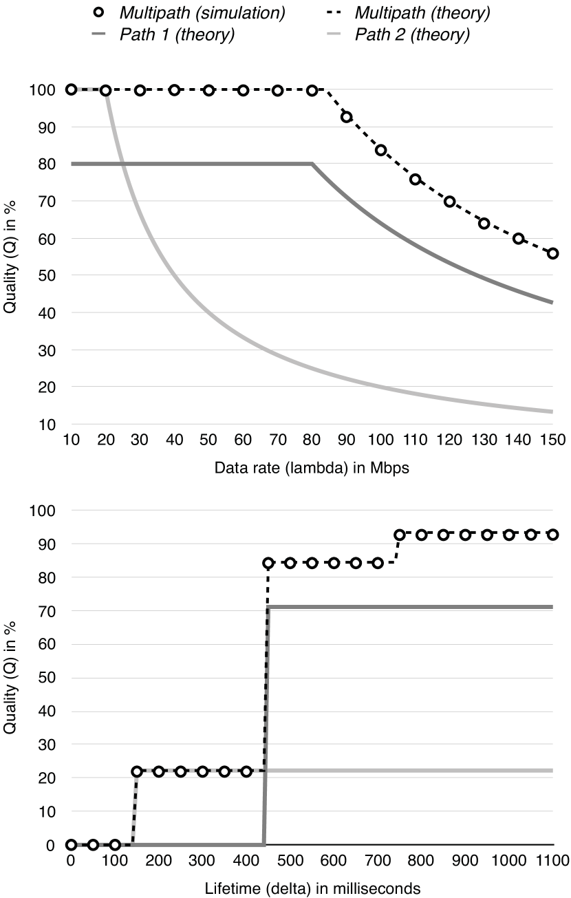
Figure 2: Theoretical and simulation results for a network with two paths. See Tables III and IV for network characteristics and solutions. $\delta=800$ milliseconds (top). $\lambda=90$ Mbps (bottom).

While Table IV shows purely theoretical performance results (and how they can be obtained), Figure 2 also shows the results of our simulation (which closely approximates the theoretical upper bound) and the maximum quality that can be achieved by using only one of the two paths.

Experiment 2: Random Delays

In this experiment, we test the random-delay extension of our model presented in Section VI in a simulation setting with two paths. We used path characteristics similar to the first experiment, but we added a random component to delay. It has been reported that packet delays along a particular Internet path can be approximated by a shifted gamma distribution [23, 24, 25, 26]. Therefore, we define delay on path $i$ as a random variable $d_{i}=X_{i}+\eta_{i}$, where $\eta_{i}$ is a location parameter and where $X_{i}$ is a random variable following a gamma distribution, i.e., with the following cumulative distribution function:

$$P(X_{i}\leq x)=\frac{\gamma(\alpha_{i},\beta_{i}x)}{\Gamma(\alpha_{i})},$$ (31)

where

$$\Gamma(\alpha)=\int_{0}^{\infty}x^{\alpha-1}e^{-x}dx$$ (32)

and

$$\gamma(\alpha,x)=\int_{0}^{x}t^{\alpha-1}e^{-t}dt.$$ (33)

Such a random variable has an expected value $\mathbb{E}[d_{i}]=\eta_{i}+\alpha_{i}\beta_{i}$ and a variance $\text{Var}[d_{i}]=\alpha_{i}\beta_{i}^{2}$.

The distribution parameters and the other network characteristics used in this simulation are shown in Table V. To minimize the effects of queueing delay and concentrate on the simulated delay distribution, we over-provisioned both paths (in terms of bandwidth), but only used the allowed amount of bandwidth ($b_{i}$) specified in the model (see Section IX-A for a discussion on queueing delays).

TABLE V: Path characteristics used in Experiment 2.

	Path 1	Path 2
Bandwidth (Mbps) $b_{i}$	80	20
Delay (ms) parameter $\eta_{i}$	400	100
Delay (ms) parameter $\alpha_{i}$	10	5
Delay (ms) parameter $\beta_{i}$	4	2
Loss rate $\tau_{i}$	0.2	0

To calculate retransmission timeouts, we use Equation 26 that we can rewrite here as

$$\begin{split}t_{i,j}=\max_{t\in\mathds{R}_{+}}(&F_{X_{j}}(\delta-\eta_{j}-t)\\ &\cdot(F_{X_{i}}(t-\eta_{i})*f_{X_{\text{min}}}(t-\eta_{\text{min}}))),\end{split}$$ (34)

where $F_{X}()$ and $f_{X}()$ denote, respectively, the cumulative distribution function and the probability density function of a random variable $X$, and $*$ stands for convolution. The above method does not necessarily produce a unique solution. In this case, the optimal timeouts that we choose are

$$\begin{gathered}t_{1,2}=615\textit{ ms},\\ t_{2,1}=252\textit{ ms},\\ t_{2,2}=323\textit{ ms}.\end{gathered}$$ (35)

The timeout $t_{1,1}$ is not defined here because it is not possible to perform a retransmission in time with that particular path combination and a lifetime of 750 ms.

In this network setting, when we generate data at a rate $\lambda=90$ Mbps, with a lifetime $\delta=750$ ms, our model extension indicates that the expected quality is $93.\overline{3}\%$ and when we used the extension in the simulation, out of 100,000 generated packets, 93,332 were received before their deadline. This indicates that the model produces realistic results and that Algorithm 1 closely approximates theoretical values in the long run.

Experiment 3: Sensitivity

Since our model requires the sender to estimate the end-to-end characteristics of the network being used (discussed in Section VIII), we analyse how sensitive the model is to inaccurate estimations. In particular, Figure 3 (top) shows how erroneous bandwidth estimation affects the communication quality when two paths are used simultaneously (with the network characteristics presented in Table III, $\lambda=90$ Mbps, $\delta=800$ milliseconds). On the left-hand side of the vertical dashed line, if the capacity of the network is underestimated, unsurprisingly, the quality decreases because the model forces packets to be dropped. On the right-hand side, however, messages are not dropped and congest the network. Therefore, the loss rate increases proportionally due to overflowing packet buffers and the communication quality remains mostly unaltered.

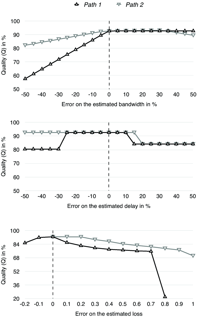
Figure 3: Simulation results showing the performance of our multipath model in function of estimation errors on the two different paths.

With regard to delay (middle of Figure 3), as expected, the quality is maximal when there is no estimation error. Moreover, there is a large plateau at the maximum quality value, which indicates that, in this particular scenario, the model is not sensitive to small ($<10$%) erroneous delay estimations.

Finally, the bottom part of Figure 3 shows that erroneously estimating loss (by a reasonable amount) also results in a small decrease in communication quality.

VIII Practical Considerations

VIII-A Estimation Techniques

The model presented above assumes that the sender has a some knowledge about the network’s characteristics. To use the model in practice, it is necessary to estimate bandwidth, delay, and loss, on each path. In this section, we discuss approaches for estimating these values in a real-world setting.

Bandwidth Estimation

The bandwidth of a network path is probably the most challenging metric to estimate, for several reasons. Firstly, bandwidth is a broad term and can refer to at least three different specific metrics in the context of data networks: capacity (maximum possible bandwidth), available bandwidth (maximum unused bandwidth), and TCP throughput or bulk transfer capacity (throughput obtainable by a single TCP connection, which is not an appropriate metric in the context of this paper) [27]. Moreover, for each of these metrics, several estimation techniques have been proposed and many tools (open source or commercial) are available, each with advantages and drawbacks. Another important aspect to consider is congestion control. TCP typically uses window-based congestion control, but other schemes based on an explicit optimization of the sending rate have been developed. For example, PCC [28] adjusts the sending rate depending on the outcome of a utility function. When the system reaches a stable state, the rate determined by the congestion control algorithm can directly be used as the value of $b_{i}$ in our model.

Delay Estimation

Estimating the average delay is relatively straightforward. As soon as an acknowledgment is received, an RTT value can be computed. However, as we assume that acknowledgments always come from the same path (the one with the lowest latency), estimating the delay of all paths requires a more elaborate acknowledgment scheme (such as the one we outline in Section VIII-C). To estimate the probability distribution $D_{i}$ that delay follows on a given path (Equation 24), two approaches are possible. First, if a specific distribution is assumed (e.g., a shifted gamma distribution), then its parameters can be estimated through regressions analysis [26]. Alternatively, the problem can be discretized by recording a sample of packet delays to determine average delays in place of expected values (Equation 25) and discrete probability distributions instead of continuous ones (Equations 26–30).

Loss Estimation

The loss rate of a path is estimated by dividing the number of lost packets by the total number of packets sent along that path. To obtain an accurate estimation, this process requires that a large number of packets have been sent. For that reason, the loss rate can first be set to 0% and the sending strategy can then be refined every time a loss is recorded.

VIII-B Complexity

There exists a profusion of libraries in various languages to solve linear programs. The time complexity of the employed algorithm is not of critical importance for the usage of our model in a protocol (since the problem size is relatively small in most practical scenarios), as long as the metric estimations are stable.

We stress that it is not necessary to solve the problem for every packet, but only when the estimations of network characteristics vary significantly. Indeed, in the best case, the problem must be solved only once—as soon as all metrics are available, and not again if metrics remain stable. However, if metrics experience volatility, or if paths go up/down, then it is important to show that solving our linear program does not constitute a heavy computational burden.

Real-valued linear programs can be solved in (worst-case) polynomial time in terms of the number of variables, with different variants of the interior-point method. However, in the case of Equation 10, the size of $x^{\prime}$ grows exponentially with the number of retransmissions considered. To be precise, for a problem with $n^{m}$ variables ($n$ being the number of paths and $m$ the number of retransmissions) and that can be encoded in L input bits, Karmarkar’s algorithm [29] requires $O(n^{(7/2)m}L)$ operations.

Our experiments with a commodity machine (2.8 GHz Intel Core i5, 8 GB 1600 MHz DDR3) and the CGAL library [22] show that, on average (calculated over 100 runs), it takes about 458.39 microseconds to solve a problem in which we consider two paths (excluding the blackhole path) and two transmissions per data unit, for example, which is negligible given that solving the problem does not block packet transmissions. Figure 4 shows computation times for larger problems (averaged over 100 runs).

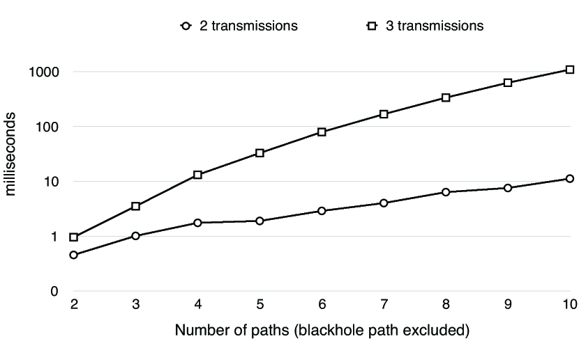
Figure 4: Computation times for solving multipath problems of different sizes (linear programming). The y-axis is in logarithmic scale.

VIII-C Acknowledgment scheme

In our model, we assume that acknowledgments cannot get lost, always take the lowest-latency path, and yet that RTT estimation is possible. One important observation is that all the data should be acknowledged through the same path the data came from for precise and accurate RTT estimation. However, this does not mean that the acknowledgment cannot also contain information about other packets that were (or were not) received on other paths.

To get as close as possible to the above-mentioned assumption in practice, the acknowledgments sent in response to every (or every $n$) packet(s) should contain a combination of the following pieces of information: (a) the range of (i.e., the lowest and the highest) packet numbers that the receiver is expecting, (b) a bit vector and its position indicating what was already received in a set of consecutive packets, (c) the packet that was just received (for RTT estimation).

In links with low bandwidth-delay products, an acknowledgement packet may contain enough information to describe the entire set of packets that are in-flight between the sender and receiver. However, when the bandwidth-delay product is large, and the lowest-latency path is lossy, the design of such acknowledgements is more complicated. Specifically, the bit vector indicating which packets have been received and which packets have not been received may be shorter than the packets in flight, for reasons such as maximum packet size and the desire to reduce overhead. In such cases, the receiver’s acknowledegment scheme becomes an integral part of reaching the desired quality metric. The goal is to create an acknowledgement stream that maximizes the quality for a given cost. However, because we do not know which acknowledgement packets will be lost, we can only maximize the expected quality, and because our acknowledgement algorithm must be nearly on-line (and therefore does not have knowledge of future acknowledgement transmission times), such quality can only be optimized with respect to a particular timing for future acknowledgements. We leave to future work the problem of designing a high-performance, low-overhead acknowledgement scheme that performs well for both low and high bandwidth-delay products.

VIII-D Retransmissions

In addition to using a retransmission timeout as described in Section VI-B, it is possible to implement a fast-retransmission mechanism (similar to TCP’s “fast retransmit” enhancement [30]), based on the fact that per-path packet re-ordering is a relatively unlikely event in the communication architecture we consider. This allows correcting for inappropriate timeout values caused by erroneous delay estimations, when the amount of generated traffic is sufficient.

In TCP, the mechanism is triggered after three duplicate acknowledgments, but no formal motivation is provided for this particular number. Therefore, the question of exactly how such a mechanism should work in our context remains open.

IX Discussion

IX-A Path Characteristics Influenced by Usage

In some cases where a path has limited resources (such as bandwidth and queue length) relative to our ability to use those resources, our usage of a path may impact the performance characteristics of that path. A mostly-saturated link, when it encounters increased traffic, may exhibit a higher loss rate than the one initially measured; likewise, queuing theory shows that as utilization increases, latency also increases. These effects introduce non-linearities in our model, since changes in $x$ affect latency and loss rates, and thus quality $p^{\text{T}}$ (Equation 11) and bandwidth usage $A$ (Equation 14). In such environments, we can initially assume that the characteristics of each path are independent of transmission rate. As long as our path usage does not change, there is no impact on our linear-programming solution. Otherwise, we gather link characteristic information as the path usage changes and determine whether a statistically significant change occurs in link characteristics. If so, we model the link’s latency and loss as a function of input bandwidth, and replace Equation 10 with a non-linear program that takes into account the impact of transmission rates on quality and bandwidth limits.

When two paths share a common subpath, traffic sent on one path can influence the properties of traffic sent along the other path. In many network architectures, we can determine that two paths are linked in this way; for example, on the Internet, traceroute may reveal the extent to which two paths share a common subpath. Detecting such situations and modifying the non-linear program appropriately is beyond the scope of this paper, and left as future work. Conveniently, our algorithm tends to send packets smoothly; that is, the inter-arrival time between two consecutive packets sent on the same path tends to be similar as long as the sending rate is smooth. As a result, our approach need not consider the impact of traffic patterns (rather than traffic amounts) on queuing latency and loss.

IX-B Channel Coding

Our model does not include any form of channel coding and focuses instead on the optimal transmission/retransmission strategy. It is established that correlated losses decrease the effectiveness of open-loop error control schemes (such as forward error correction) and experiments showed that losses are correlated even when as little as 10% of capacity is used [31]. Although there might be an opportunity to de-correlate losses by sending consecutive packets along different paths, that approach has limitations. When a packet is lost, the delay required to recover the corresponding group of packets equals the longest delay of all paths. Therefore, the benefits of end-to-end coding (including in a multipath context) are questionable and need to be further investigated. Moreover, in terms of fairness to other users/applications, only performing retransmissions with no additional redundancy (due to coding) is more desirable.

IX-C Interpretation of Bandwidth and Cost Limits

Our model operates on the expected value of the bandwidth to be used and the cost bound. In particular, the values in $A$ (Equation 14) use the traffic vector to calculate the expected usage of each link and the expected cost. In some systems, exceeding a user-specified cost bound may be unacceptable; in other systems, exceeding the pre-specified bandwidth limits may result in packet loss that cannot be handled by our model. In such cases, a system using our approach can adjust the values in $q$ (Equation 17) until an acceptable solution is reached. In particular, given a certain data rate, number of packets, and rate solution $x^{\prime}$, we can compute the probability of exceeding an expected cost or a bandwidth limit; in the event that this probability is too high, the system can adjust the bandwidth limit or cost limit and re-solve the linear program to obtain a solution that is closer to the system’s goals.

X Conclusion

Packet switching has the advantage of enabling the usage of several network paths simultaneously for a single stream of data or even for a single message, which constitutes an attractive research area for improving network performance. Unfortunately, the path diversity that the Internet offers is rarely fully exploited, for several reasons. First, the current Internet architecture does not allow end hosts to specify the path(s) they want to use. Second, the multipath paradigm poses many new challenges and requires that most transport-layer concepts be redesigned. Finally, the advantages that multipath communication offers are not well known because they have not yet been sufficiently examined.

In this paper, we proposed an analytical model for optimizing the performance of partially-reliable multipath communications, in particular with the goal of developing better protocols for latency-sensitive applications. We showed that path diversity achieves better performance than uniform paths in deadline-based scenarios, through theoretical and simulation results. Many challenges remain to design a deployable protocol (e.g., cross traffic, varying conditions, congestion/flow control), which we leave to be addressed by future work. However, multipath communication promises to provide a multitude of desirable properties.

References

- [1] C. Raiciu, C. Paasch, S. Barre, A. Ford, M. Honda, F. Duchene, O. Bonaventure, and M. Handley, “How hard can it be? designing and implementing a deployable multipath TCP,” in Proceedings of the 9th USENIX conference on Networked Systems Design and Implementation (NSDI), 2012.
- [2] A. Singla, B. Chandrasekaran, P. B. Godfrey, and B. Maggs, “The Internet at the speed of light,” in Proceedings of the 13th ACM Workshop on Hot Topics in Networks (HotNets), 2014.
- [3] A. Hern, “Facebook launches Aquila solar-powered drone for Internet access,” August 2015. [Online]. Available: https://www.theguardian.com/technology/2015/jul/31/facebook-finishes-aquila-solar-powered-internet-drone-with-span-of-a-boeing-737
- [4] “Google begins launching Internet-beaming balloons,” June 2013. [Online]. Available: http://news.temple.edu/in-the-media/google-begins-launching-internet-beaming-balloons
- [5] T. Fernholz, “The details behind SpaceX’s ambitious satellite Internet experiment,” June 2015. [Online]. Available: https://qz.com/426158/the-details-behind-spacexs-ambitious-satellite-internet-experiment/
- [6] X. Zhang, H.-C. Hsiao, G. Hasker, H. Chan, A. Perrig, and D. G. Andersen, “SCION: Scalability, control, and isolation on next-generation networks,” in Proceedings of the IEEE Symposium on Security and Privacy (S&P), May 2011.
- [7] T. Anderson, K. Birman, R. Broberg, M. Caesar, D. Comer, C. Cotton, M. J. Freedman, A. Haeberlen, Z. G. Ives, A. Krishnamurthy, W. Lehr, B. Loo, D. Mazieres, A. Nicolosi, J. M. Smith, I. Stoica, R. Renesse, M. Walfish, H. Weatherspoon, and C. S. Yoo, “The NEBULA future Internet architecture,” in The Future Internet, 2013.
- [8] C. Filsfils, N. K. Nainar, C. Pignataro, J. C. Cardona, and P. Francois, “The segment routing architecture,” in Proceedings of the IEEE Global Communications Conference (GLOBECOM), 2015.
- [9] X. Yang, D. Clark, and A. W. Berger, “NIRA: A new inter-domain routing architecture,” IEEE/ACM Transactions on Networking, July 2007.
- [10] P. B. Godfrey, I. Ganichev, S. Shenker, and I. Stoica, “Pathlet routing,” in Proceedings of the ACM SIGCOMM Conference, 2009.
- [11] N. P. Lago and F. Kon, “The quest for low latency,” in Proceedings of the International Computer Music Conference (ICMC), 2004.
- [12] “YouTube live streaming API overview.” [Online]. Available: https://developers.google.com/youtube/v3/live/getting-started
- [13] B. Vamanan, J. Hasan, and T. N. Vijaykumar, “Deadline-aware datacenter TCP (D2TCP),” in Proceedings of the ACM SIGCOMM Conference, 2012.
- [14] R. Stewart, M. Ramalho, Q. Xie, M. Tuexen, and P. Conrad, “Stream control transmission protocol (SCTP) partial reliability extension,” RFC 3758, May 2004.
- [15] R. Stewart, M. Tuexen, and P. Lei, “SCTP: What is it, and how to use it?” in Proceedings of BSDCan: The Technical BSD Conference, 2008.
- [16] X. Liu, S. Mohanraj, M. Pioro, and D. Medhi, “Multipath routing from a traffic engineering perspective: How beneficial is it?” in Proceedings of the 22nd IEEE International Conference on Network Protocols (ICNP), 2014.
- [17] P. Soldati, H. Zhang, Z. Zou, and M. Johansson, “Optimal routing and scheduling of deadline-constrained traffic over lossy networks,” in Proceedings of the IEEE Global Communications Conference (GLOBECOM), 2010.
- [18] J. Wu, C. Yuen, B. Cheng, Y. Shang, and J. Chen, “Goodput-aware load distribution for real-time traffic over multipath networks,” IEEE Transactions on Parallel and Distributed Systems, August 2015.
- [19] C. Cetinkaya and E. W. Knightly, “Opportunistic traffic scheduling over multiple network paths,” in Proceedings of the IEEE International Conference on Computer Communications (INFOCOM), 2004.
- [20] S. Prabhavat, H. Nishiyama, N. Ansari, and N. Kato, “Effective delay-controlled load distribution over multipath networks,” IEEE Transactions on Parallel and Distributed Systems, January 2011.
- [21] T. R. Henderson, M. Lacage, G. F. Riley, C. Dowell, and J. Kopena, “Network simulations with the ns-3 simulator,” SIGCOMM demonstration, August 2008.
- [22] “The computational geometry algorithms library (CGAL).” [Online]. Available: http://www.cgal.org/
- [23] A. Mukherjee, “On the dynamics and significance of low frequency components of Internet load,” Internetworking: Research and Experience, December 1992.
- [24] V. Paxson, “End-to-end Internet packet dynamics,” IEEE/ACM Transactions on Networking, June 1999.
- [25] S. Kim, J. Y. Lee, and D. K. Sung, “A shifted gamma distribution model for long-range dependent Internet traffic,” IEEE Communications Letters, March 2003.
- [26] D. Chen, X. Fu, W. Ding, H. Li, N. Xi, and Y. Wang, “Shifted gamma distribution and long-range prediction of round trip timedelay for Internet-based teleoperation,” in Proceedings of the IEEE International Conference on Robotics and Biomimetics (ROBIO), 2009.
- [27] R. Prasad, C. Dovrolis, M. Murray, and K. Claffy, “Bandwidth estimation: metrics, measurement techniques, and tools,” IEEE Network, November 2003.
- [28] M. Dong, Q. Li, D. Zarchy, P. B. Godfrey, and M. Schapira, “PCC: Re-architecting congestion control for consistent high performance,” in Proceedings of the 12th USENIX Symposium on Networked Systems Design and Implementation (NSDI), 2015.
- [29] G. Strang, “Karmarkar’s algorithm and its place in applied mathematics,” The Mathematical Intelligencer, June 1987.
- [30] M. Allman, V. Paxson, and W. Stevens, “TCP congestion control,” RFC 2581, April 1999.
- [31] J.-C. Bolot, “Characterizing end-to-end packet delay and loss in the Internet,” Journal of High Speed Networks, July 1993.