Sparse Neural Network Topologies

Abstract

We propose Sparse Neural Network architectures that are based on random or structured bipartite graph topologies. Sparse architectures provide compression of the models learned and speed-ups of computations, they can also surpass their unstructured or fully connected counterparts. As we show, even more compact topologies of the so-called SNN (Sparse Neural Network) can be achieved with the use of structured graphs of connections between consecutive layers of neurons.

In this paper, we investigate how the accuracy and training speed of the models depend on the topology and sparsity of the neural network. Previous approaches using sparcity are all based on fully connected neural network models and create sparcity during training phase, instead we explicitly define a sparse architectures of connections before the training. Building compact neural network models is coherent with empirical observations showing that there is much redundancy in learned neural network models. We show experimentally that the accuracy of the models learned with neural networks depends on ”expander-like” properties of the underlying topologies such as the spectral gap and algebraic connectivity rather than the density of the graphs of connections.

1 Introduction

The last decade has seen a rapid development of neural network methods that are widely considered to be the best tools for solving hard machine learning problems such as speech [1],[2], [3], image [4], [5], [6] and video [7],[8] recognition. Neural networks are believed to learn complex models by iterating two operations: linear projections of high-dimensional data and pointwise nonlinear mappings.

However, the process of building a good quality neural network models is time-consuming and the models’ space complexity is usually very high. In this paper, we investigate how the quality of the neural network model depends on the topology of connections between consecutive layers. We propose Sparse Neural Network (SNN) architectures that can match or exceed the accuracy of their dense counterparts. First, we study random sparse architectures that are quite compressible, then we study similar structured versions that provide even more compact description of the entire architecture. Sparse structured graphs are highly-compressible, yet they can share some properties with their sparse random counterparts. We show good quality SNN model, with a well chosen topology, can equal or supersede its fully connected equivalent in accuracy, with a much smaller learned parameter space. We also show that our results our robust as they hold over multiple layer neural network, or with the use of some over-fitting prevention techniques such as Dropout [9]. There is also additional insight into Neural Network inner workings and limitations by implementing SNN’s and viewing them through the lens of graphs. We investigate how Algebraic Connectivity impacts a Neural Network’s power, and show that there is a strong correlation between how interconnected a Neural Network is, and its resulting testing accuracy.

2 Related work

It was recently observed [10], [11], [12] that imposing specific structure of the linear embedding part of the neural network computations leads to significant speed-ups and memory usage reductions with only minimal loss of the quality of the model. In this approach, the graph of connections between consecutive neural network layers is still dense and the reduction comes from recycling a compact vector of learned weights across the entire matrix.

In [13] the authors use a compact multilinear format, called the Tensor-Train format to represent the dense weight matrix of the fully-connected layers. Even more basic technique relies on using the low-rank representation of the weight matrices. It was empirically tested that restricting the rank of the matrix of neurons connections to be of low rank does not affect much the quality of the model [14], [15], [16], [17]. This setting is more restrictive than the one presented in [10], since low-rank matrices considered in these papers have in particular low displacement rank.

Other sets of techniques, such as methods exploting the so-called HashedNets architectures, incorporate specific hashing tricks based on easily-computable hash functions to group weights connections into hash buckets. This procedure significantly reduces the size of the entire model. Some other methods involve applying certain clustering and quantization techniques to fully-connected layers [18] that, as reported, have several advantages over existing matrix factorization methods.

Sparse neural network architectures were studied before, but in a different context. Good quality deep neural network/energy-based models might be obtained by imposing sparsity restrictions with nonzero activations [19], [20], [21] or using a linear rectifier as a nonlinear mapping. Sparsity was also studied in the case of Dropout[9] and DropConnect [22] features where random vertices or edges are deactivated at each training batch to prevent over-fitting.

However, all of these architectures are based on a fully connected neural network that is sparsified during the training phase. Our goal is not to deactivate many neurons or connection in the training phase by applying a particular regularization to the cost function, but rather to sparsify the graph of connections before. Our setting allows for speed up computations from the very beginning of the training phase due to the fact that sparse matrix - vector multiplication can be conducted much faster than its dense matrix - vector multiplication counterpart.

3 Constructing sparse random and structured topologies

We focus here on defining adjacency matrices of bipartite graphs between consecutive layers in the fixed neural network architecture. Assuming that the $l^{th}$ layer consists of $n$ neurons and the $(l+1)^{th}$ layer consists of $m$ neurons, we consider the standard unweighted $n\times m$ adjacency matrix $\textit{Adj}_{l}\in\mathbb{R}^{n\times m}$, where:

$$Adj_{l}[i][j]=\left\{\begin{array}[]{ll}1&\mbox{if }(i,j)\in E_{l},\\ 0&\mbox{otherwise,}\end{array}\right.$$ (1)

$E_{l}$ denotes the set of edges of the corresponding bipartite graph and $(i,j)$ stands for the edge between $i^{th}$ neuron in the $l^{th}$ layer and $j^{th}$ neuron in the $(l+1)^{th}$ layer.

Defined above adjacency matrix is then applied element-wise to the weight matrix at the respective layer at each update, effectively zeroing out the non-desired connection. Let $\delta_{l}$ denote the expected degree of the neuron in the $l^{th}$ layer, i.e. $\delta_{l}=\mathbb{E}[\sum_{j=1^{m}}\textit{Adj}[i][j]$. To obtain satisfactory compression rates for our SNN, we set: $\delta_{l}<m$.

Below we present specific structured topologies applied in our SNN as well as sparse unstructured topologies that were the subject of our analysis.

3.1 Random Constructions

3.1.1 Random Edge Construction

This is the most straight forward construction, where each node from the first layer is connected to independently chosen random set of nodes in the second layer, or to be more specific:

$$P[Adj[i][j]=1]=k/m$$

for some fixed parameter $k$. Notice that the number of edges of such a random bipartite graph has expectation $nk$ and highly concentrated around this expectation.

3.1.2 Random Rotating Edge Construction

In this construction, an edge matrix is created by a random binary vector of length $m$, and rotated at each row in a circulant fashion. The rotating vector is filled by assigning a connection with probability

$$P[Adj[i][0]=1]=k/m$$

And we rotate this vector to get the connection matrix.

$$Adj[i][j^{\prime}]=Adj[i][j]\ where\ j^{\prime}=j-i\ mod\ m$$

To ensure the expected degree is in line with other constructions, we also fix the number of connections in the initial construction to be sure to have exactly $k$ connections.

3.1.3 Random d-Regular Expander Construction

In this construction, an approximated bipartite expander graph is created. Each vertex from the input (or left layer) has a fixed degree $D=k/m$, meaning exactly $D$ connections with the output or right layer. The connections are then randomly assigned to the right layer, giving the random graph a high probability that it is an expander. For more details on probabilistic constant degree expanders refer to [23]

3.2 Structured Constructions

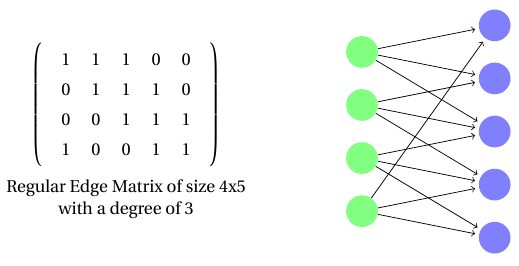
3.2.1 Regular Rotating Edge Construction

In this construction, the deterministic vector of length $m$ is created by simply having $k$ ones followed by $m-k$ zeroes.

$$Adj[i][j]=1\ for\ i\ mod\ m<j<i+k\ mod\ m,\ 0\ otherwise$$

This construction is particularly interesting due to its rigid structure, allowing for a better computing time, and a smaller memory space used. The edge matrix and its related graph is presented in the figure below.

Figure 1: Experiments Results

3.2.2 Long-Short Rotating Edge Construction

In this construction, a deterministic vector of length $m$ is created by having $k/2$ ones followed by $k/2$ ones regularly placed between the $m-k/2$ positions left. The motivation being that connectedness of far away neurons allows for more information mixing and better accuracy than simple regular rotating edge construction.

3.2.3 Fibonnaci Rotating Edge Construction

In this construction, a deterministic vector on length $m$ is created by using the $k$ first Fibonacci numbers. If the $k^{th}$ Fibonacci number is smaller than $m$, we create a connection if the index is in the Fibonacci list. We also fill the zero index with the 1st one of the Fibonacci list. If the $k^{th}$ Fibonacci number is bigger than m, we normalize our list by multiplying it with $m/Fibo(k)$. With this transformation, we get a list of float numbers. To be certain that we will have exactly $k$ ones in the vector, we fill the next element if the current value is already one. This vector is then rotated in a similar fashion as the previous deterministic constructions to produce the edge matrix.

4 Experimental Results

4.1 Experimental Setup

In order to investigate how sparsity impacts performance, we use the canonical MNIST database of 60,000 handwritten digits images as the training set, and an additional 10,000 images as the test set. The neural architecture we use is one hidden layer of size 100, 300, or 500, with the conventional flattened 28*28 input and 10 output layer size. We then train many networks with the varying constructions described above and varying degree k imposed on both the input to hidden layer connection and hidden layer to output, fitting a total of 3000 networks. We train each network for 50 epochs with a fixed batch size of 32. We use mean square error as the loss function, the initialization function is a Glorot Gaussian [24]. A standard stochastic gradient descent optimizer is used with Nesterov momentum of 0.9 and learning rate of 1%. The activation function at all neurons is a regular sigmoid. Implementation was achieved using the python package Keras[25] with Theano[26][27] as a backend. We then modify the update steps to impose sparsity at each step as described previously.

4.2 Sparse Neural Nets Perform Well

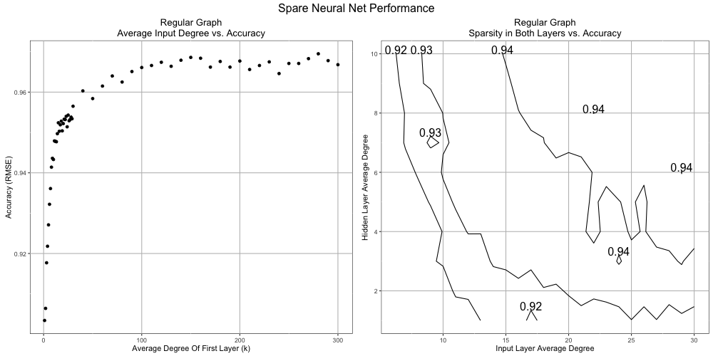
A key finding is that at very low levels of imposed sparsity, SNN can perform as well as their Fully Connected counterparts. In Figure 2, one can see that there is no precipitous drop off of accuracy until well below 10% of the connections remain while varying the expected degree $k$ of the input layer to the hidden layer. This result is consistent with varying the expected degree of the hidden layer as well, as seen in the contour plot of Figure 2. The experiments depicted are with a hidden layer of 300 and with a regular graph construction for simplicity, but the same result holds for all constructions and hidden layer sizes.

Figure 2: Experimental Results of a Regular Graph Construction with Hidden Layer Size 300

4.3 Sparse Constructions Perform Differently

Another key result is that different sparse architectures with the same degree of connection don’t result in the same accuracy. In Figure 3, one can see how constructions vary in performance at very sparse levels on the left, as well as for increasing levels of connectedness on the right. In some cases, such as the structured Regular and Fibonacci constructions, the SNN outperforms its fully connected counterpart, indicating a better fitted model as a result of reducing the parameter space. The reason might be that big fully connected networks are worse at handling the noise because of their very redundant connections. Also, in a subsequent section we discuss how algebraic connectivity could be a possible way to predict this result.

Figure 3: Varying Performance of Neural Net Construction

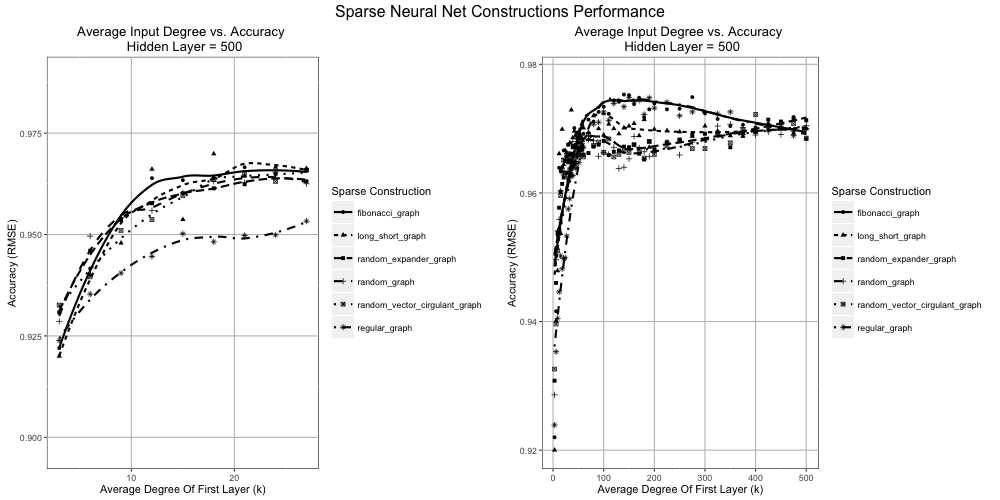
Overall, the Fibonacci SNN seems to be the best choice of structure. Indeed, it’s the only SNN that is both pseudo regular (which gives in good and sometimes better accuracy in the sparse setting) and pseudo random (which avoid sharp drop in accuracy if the network is very sparse). Regular SNN is a good second choice since it provides equivalently good results in most cases with a simpler implementation.

4.4 The Results Hold With Dropout or Deeper Networks

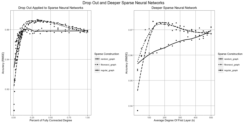
As previously discussed, over fitting is a big issue with neural networks and dropout methodology is extensively used to prevent this problem. We experimented with both sparsifying methods. We augmented our methodology of a SNN architecture which is set from the beginning with [9]methodology of dropping a fixed number of vertices at each learning batch to avoid over fitting. With dropout=0.2 for the input layer and dropout=0.5 for the hidden layer, we show that the two methods are independent in Figure 4. The sparse Fibonacci and Regular networks still have a better accuracy than that of the fully connected equivalent.

As neural networks rarely have only one hidden layer, and are becoming deeper with the increase in computing power we studied SNN with two hidden layers. In this setting, the structured Regular or Fibonacci SNN still performs better than its fully connected network equivalent. In Figure 4, we also present the results for a network of size 784-500-300-10 with the degrees of the two hidden layers varying at the same pace and the last layer being fully connected. In this case, the regular and Fibonacci sparse neural network still perform better than their fully connected equivalent. With only 30% connections in the network, we are able to increase accuracy by 0.15% after the same number of training epochs.

Figure 4: Sparse Constructions in Different Settings

4.5 Graph Properties and Accuracy

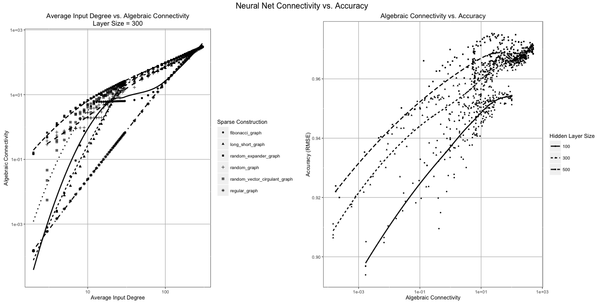
After training these SNN, there is a need to measure what causes the differences between topologies, and how graphical properties are related to the resulting accuracy. Two critical measures we identify are spectral gap and algebraic connectivity, which are defined as the first and second largest non-zero eigen value of the Laplacian matrix respectively. We find that connectivity varies between constructions substantially, particularly in the very sparse regimes, which can bee seen below. Hand in hand with this observation is connectivity is highly correlated with accuracy. When determining how to design a SNN topology, connectivity is a critical parameter to consider when constructing it.

Figure 5: Connectivity of various constructions, and its relationship to accuracy

4.6 Sparse Neural Network Learned Weights

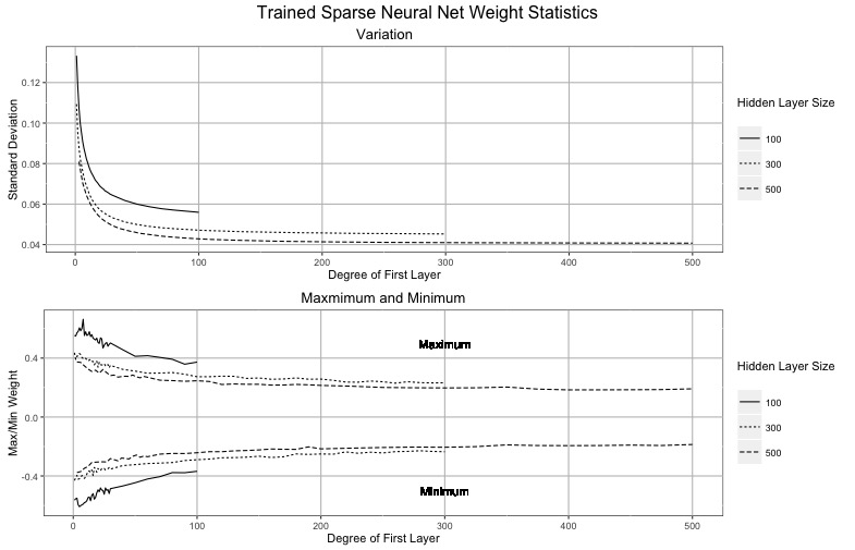
It is also interesting to look at how the learned weights vary with sparsity. While construction doesn’t have a particularly large impact on what the magnitude and distribution of the learned weights are, sparsity does. The more connections there are the more tempered the distributions become, finally leveling off at an equilibrium that reflects the same pattern that the overall accuracy of the SNN follows. The maximum, minimum and standard deviation of the connected weights lower with respect to both hidden layer size and degree connectivity. This follows intuition: the less weights you have, the more critical and high valued they become.

Figure 6: Trained Sparse Neural Net Weight Statistics

5 Conclusion and Future Work

We have shown that SNN (Sparse Neural Network) constructions can be as competitive as, and sometimes outperform their fully connected counterparts with also shorter training time. The SNN can outperform its fully connected equivalent in the case of structured SNN such as a Regular or Fibonacci, with medium sparcity on large hidden layers. Overall, Fibonacci SNN different from Regular SNN as they are more accurate in very sparse setting (less than 10% connections), but regular SNN also provide much simpler implementation.

We empirically verified that the accuracy of the sparse topologies depend on ”expander-like” properties of the matrix such as its algebraic connectivity. Much future work remains to further expand on the findings of this paper, such as applying the same techniques to other neural network architectures (i.e. as CNN, LSTM). This paper opens an orthogonal direction of study that promises interesting advances in neural network’s understanding and adds new tools to the neural network tool kit. It could eventually be employed to fit better models or provide tools for resources constrained applications such as connected and mobile devices.

References

- [1] Alex Graves, Abdel-rahman Mohamed, and Geoffrey E. Hinton. Speech recognition with deep recurrent neural networks. In IEEE International Conference on Acoustics, Speech and Signal Processing, ICASSP 2013, Vancouver, BC, Canada, May 26-31, 2013, pages 6645–6649, 2013.
- [2] Alexander H. Waibel, Toshiyuki Hanazawa, Geoffrey E. Hinton, Kiyohiro Shikano, and Kevin J. Lang. Phoneme recognition using time-delay neural networks. IEEE Trans. Acoustics, Speech, and Signal Processing, 37(3):328–339, 1989.
- [3] Ruhi Sarikaya, Geoffrey E. Hinton, and Anoop Deoras. Application of deep belief networks for natural language understanding. IEEE/ACM Trans. Audio, Speech & Language Processing, 22(4):778–784, 2014.
- [4] Yann LeCun, Patrick Haffner, Léon Bottou, and Yoshua Bengio. Object recognition with gradient-based learning. In Shape, Contour and Grouping in Computer Vision, page 319, 1999.
- [5] Alex Krizhevsky, Ilya Sutskever, and Geoffrey E. Hinton. Imagenet classification with deep convolutional neural networks. In Advances in Neural Information Processing Systems 25: 26th Annual Conference on Neural Information Processing Systems 2012. Proceedings of a meeting held December 3-6, 2012, Lake Tahoe, Nevada, United States., pages 1106–1114, 2012.
- [6] Dan Claudiu Ciresan, Ueli Meier, Luca Maria Gambardella, and Jürgen Schmidhuber. Deep, big, simple neural nets for handwritten digit recognition. Neural Computation, 22(12):3207–3220, 2010.
- [7] Andrej Karpathy, George Toderici, Sanketh Shetty, Thomas Leung, Rahul Sukthankar, and Fei-Fei Li. Large-scale video classification with convolutional neural networks. In 2014 IEEE Conference on Computer Vision and Pattern Recognition, CVPR 2014, Columbus, OH, USA, June 23-28, 2014, pages 1725–1732, 2014.
- [8] Karen Simonyan and Andrew Zisserman. Two-stream convolutional networks for action recognition in videos. In Advances in Neural Information Processing Systems 27: Annual Conference on Neural Information Processing Systems 2014, December 8-13 2014, Montreal, Quebec, Canada, pages 568–576, 2014.
- [9] Nitish Srivastava, Geoffrey E. Hinton, Alex Krizhevsky, Ilya Sutskever, and Ruslan Salakhutdinov. Dropout: a simple way to prevent neural networks from overfitting. Journal of Machine Learning Research, 15(1):1929–1958, 2014.
- [10] V. Sindhwani, T. Sainath, and S. Kumar. Structured transforms for small-footprint deep learning. In NIPS, 2015.
- [11] Yu Cheng, Felix X. Yu, Rogerio S. Feris, Sanjiv Kumar, Alok Choudhary, and Shih-Fu Chang. An exploration of parameter redundancy in deep networks with circulant projections. In arXiv:1502.03436, 2015.
- [12] Vamsi Sashank Kotagiri. Memory capacity of neural networks using a circulant weight matrix. In arXiv:1403.3115, 2014.
- [13] Alexander Novikov, Dmitry Podoprikhin, Anton Osokin, and Dmitry Vetrov. Tensorizing neural networks. CoRR, abs/1509.06569, 2015.
- [14] Tara N. Sainath, Brian Kingsbury, Vikas Sindhwani, Ebru Arisoy, and Bhuvana Ramabhadran. Low-rank matrix factorization for deep neural network training with high-dimensional output targets. In IEEE International Conference on Acoustics, Speech and Signal Processing, ICASSP 2013, Vancouver, BC, Canada, May 26-31, 2013, pages 6655–6659, 2013.
- [15] Jian Xue, Jinyu Li, and Yifan Gong. Restructuring of deep neural network acoustic models with singular value decomposition. In INTERSPEECH 2013, 14th Annual Conference of the International Speech Communication Association, Lyon, France, August 25-29, 2013, pages 2365–2369, 2013.
- [16] Misha Denil, Babak Shakibi, Laurent Dinh, Marc’Aurelio Ranzato, and Nando de Freitas. Predicting parameters in deep learning. In Advances in Neural Information Processing Systems 26: 27th Annual Conference on Neural Information Processing Systems 2013. Proceedings of a meeting held December 5-8, 2013, Lake Tahoe, Nevada, United States., pages 2148–2156, 2013.
- [17] Cheng Tai, Tong Xiao, Xiaogang Wang, and Weinan E. Convolutional neural networks with low-rank regularization. CoRR, abs/1511.06067, 2015.
- [18] Yunchao Gong, Liu Liu, Ming Yang, and Lubomir D. Bourdev. Compressing deep convolutional networks using vector quantization. CoRR, abs/1412.6115, 2014.
- [19] Xavier Glorot, Antoine Bordes, and Yoshua Bengio. Deep sparse rectifier neural networks. In Proceedings of the Fourteenth International Conference on Artificial Intelligence and Statistics, AISTATS 2011, Fort Lauderdale, USA, April 11-13, 2011, pages 315–323, 2011.
- [20] Honglak Lee, Chaitanya Ekanadham, and Andrew Y. Ng. Sparse deep belief net model for visual area V2. In Advances in Neural Information Processing Systems 20, Proceedings of the Twenty-First Annual Conference on Neural Information Processing Systems, Vancouver, British Columbia, Canada, December 3-6, 2007, pages 873–880, 2007.
- [21] Marc’Aurelio Ranzato, Christopher S. Poultney, Sumit Chopra, and Yann LeCun. Efficient learning of sparse representations with an energy-based model. In Advances in Neural Information Processing Systems 19, Proceedings of the Twentieth Annual Conference on Neural Information Processing Systems, Vancouver, British Columbia, Canada, December 4-7, 2006, pages 1137–1144, 2006.
- [22] Li Wan, Matthew D. Zeiler, Sixin Zhang, Yann LeCun, and Rob Fergus. Regularization of neural networks using dropconnect. In Proceedings of the 30th International Conference on Machine Learning, ICML 2013, Atlanta, GA, USA, 16-21 June 2013, pages 1058–1066, 2013.
- [23] Michael Capalbo, Omer Reingold, Salil Vadhan, and Avi Wigderson. Randomness conductors and constant-degree lossless expanders. In Proceedings of the Thiry-fourth Annual ACM Symposium on Theory of Computing, STOC ’02, pages 659–668, New York, NY, USA, 2002. ACM.
- [24] Xavier Glorot and Yoshua Bengio. Understanding the difficulty of training deep feedforward neural networks. In International conference on artificial intelligence and statistics, pages 249–256, 2010.
- [25] Fran ois Chollet. keras. https://github.com/fchollet/keras, 2015.
- [26] James Bergstra, Olivier Breuleux, Frédéric Bastien, Pascal Lamblin, Razvan Pascanu, Guillaume Desjardins, Joseph Turian, David Warde-Farley, and Yoshua Bengio. Theano: a CPU and GPU math expression compiler. In Proceedings of the Python for Scientific Computing Conference (SciPy), June 2010. Oral Presentation.
- [27] Frédéric Bastien, Pascal Lamblin, Razvan Pascanu, James Bergstra, Ian J. Goodfellow, Arnaud Bergeron, Nicolas Bouchard, and Yoshua Bengio. Theano: new features and speed improvements. Deep Learning and Unsupervised Feature Learning NIPS 2012 Workshop, 2012.