Resource Optimization and Power Allocation in In-band Full Duplex (IBFD)-Enabled Non-Orthogonal Multiple Access Networks

Abstract

In this paper, the problem of uplink (UL) and downlink (DL) resource optimization, mode selection and power allocation is studied for wireless cellular networks under the assumption of in-band full duplex (IBFD) base stations, non-orthogonal multiple access (NOMA) operation, and queue stability constraints. The problem is formulated as a network utility maximization problem for which a Lyapunov framework is used to decompose it into two disjoint subproblems of auxiliary variable selection and rate maximization. The latter is further decoupled into a user association and mode selection (UAMS) problem and a UL/DL power optimization (UDPO) problem that are solved concurrently. The UAMS problem is modeled as a many-to-one matching problem to associate users to small cell base stations (SBSs) and select transmission mode (half/full-duplex and orthogonal/non-orthogonal multiple access), and an algorithm is proposed to solve the problem converging to a pairwise stable matching. Subsequently, the UDPO problem is formulated as a sequence of convex problems and is solved using the concave-convex procedure. Simulation results demonstrate the effectiveness of the proposed scheme to allocate UL and DL power levels after dynamically selecting the operating mode and the served users, under different traffic intensity conditions, network density, and self-interference cancellation capability. The proposed scheme is shown to achieve up to 63% and 73% of gains in UL and DL packet throughput, and 21% and 17% in UL and DL cell edge throughput, respectively, compared to existing baseline schemes.

I Introduction and related work

Due to the rapid increase in the demand for wireless data traffic, there has been substantial recent efforts to develop new solutions for improving the capacity of wireless cellular networks, by enhancing the access to the scarce radio spectrum resources [1]. In view of the scarcity of the frequency resources, smart duplexing, resource allocation, and interference management schemes are crucial to utilize the available resources in modern cellular networks and satisfy the needs of their users.

In-band full duplex (IBFD) communication has the potential of doubling the resource utilization of cellular networks through transmitting in the uplink (UL) and downlink (DL) directions using the same time and frequency resources. However, this comes at the cost of experiencing higher levels of interference, not the least of which is the self-interference (SI) leaked from the transmitter to the receiver of a IBFD radio. Moreover, IBFD cellular networks suffer from additional interference generated from having base stations and users transmitting on the same channel. These interference types, namely, DL-to-UL interference and UL-to-DL interference significantly degrade the performance of IBFD networks. Figure 1 (a) illustrates desired and interference signals in a FD-enabled base station.

Recent results have shown significant advances in the SI cancellation of wireless IBFD radios, putting full duplex (FD) operation in wireless cellular networks within reach. By employing a combination of analog and digital cancellation techniques [2, 3], it was shown that as much as $110$ dB of SI cancellation is achieved. Another approach to avoid SI is to emulate a FD base station using two spatially separated and coordinated half duplex (HD) base stations [4]. The performance of FD is investigated in [5, 6] using tools from stochastic geometry. In [5], the combined effect of SI and FD interference is analyzed. Throughput analysis are conducted in [6] with respect to network density, interference and SI levels. A system-level simulation study of the performance of IBFD ultra-dense small cell networks is conducted in [7]. The study concludes that FD may be useful for asymmetric traffic conditions. However, none of these studies take into account user selection and power allocation, which are key factors to mitigate interference in a IBFD environment.

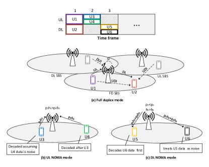
Figure 1: An illustration of (a) FD (b) UL NOMA and (c) DL NOMA operations, UDI: UL-to-DL interference, DUI: DL-to-UL interference and SI: self-interference.

To further increase the utilization of frequency resources, the possibility of multiple users sharing the same channel by exploiting differences in the power domain has recently been proposed in the context of non-orthogonal multiple access (NOMA) [8]. Different from orthogonal multiple access (OMA) schemes, NOMA allows multiple users to occupy the same channel, whereas multi-user detection methods, such as successive interference cancellation (SIC) are used to decode users’ messages [9]. In DL NOMA, users with higher channel gains can decode and cancel messages of users with lower channel gains before decoding their own messages, whereas users with lowest channel gains decode their messages first, treating other users’ messages as noise. In UL NOMA, base station performs successive decoding and cancellation of different users data, ranked by their channel strength. The UL and DL NOMA operation is illustrated for a two-user case in Figure 1 (b) and (c), respectively. The decoding order as well as the power allocation are key factors that affect the performance of NOMA. Since NOMA comes with an additional receiver complexity for the decoding phase, practical limitations on the maximum number of users operating in NOMA must be considered. The combination of UL NOMA and SIC has been shown to also enhance the cell-edge user throughput in [10].

User scheduling and power optimization are crucial factors in achieving the promised gains of both FD and NOMA schemes. Intra-cell and inter-cell cross-link interference occur due to IBFD operation. Therefore, smart resource and interference management schemes are needed to reap the gains of FD and NOMA operation. In [11], a hybrid HD/FD scheduler is proposed that can assign FD resources only when it is advantageous over HD resource assignment. An auction-based algorithm to pair UL and DL users in a single-cell IBFD network is proposed in [12]. User scheduling and power allocation algorithms are presented for IBFD networks in [13] and for DL NOMA networks in [14, 15, 16]. In the proposed approach of [14], a many-to-many matching algorithm is used to assign channel to users in a single cell scenario. The performance of NOMA in the UL is investigated in [17] using an iterative channel allocation algorithm. All of the above works focus on single-cell optimization and hence, avoid handling the inter-cell interference. A distributed sub-optimal algorithm for the problem of user selection and power allocation in a multi-cell full duplex network discussed in [18] showing that IBFD can achieve up to double the throughput of HD in indoor scenarios and $65\%$ in outdoor scenarios. However, the proposed algorithm relies on information exchange between neighboring base stations. It also does not take into account queue state information (QSI), which has a significant impact on the user packet throughput. Several algorithms are proposed in [19, 20, 21] to optimize user pairing/scheduling, and power allocation. These algorithms are either centralized or inter-cell interference is overlooked. In [22], the authors consider a multi-cell UL and DL NOMA system where they propose a user grouping and power optimization framework. The optimal power allocation is derived for a single macro cell and limited number of users. The problem of UL/DL decoupled user association is studied in [23] for multi-tier IBFD networks where many-to-one matching algorithms are proposed to solve the problem. However, dynamic user scheduling and power allocation are not considered in the optimization problem. Studying the operation of both FD and NOMA was first considered in [24], where the problem of subcarrier and power allocation in a multicarrier and single-cell FD-NOMA system is optimized. Taking into account the user traffic dynamic in the optimization problem is also missing in the literature. A summary of the state of the art contributions to FD and NOMA resource and power optimization problems is provided in Table I.

I-A Paper Contribution

The main goal of this paper is to study the problem of user association and power allocation in a multi-cell IBFD-enabled network operating in NOMA. Our objective is to investigate the benefits of operating in HD or FD, as well as in OMA or NOMA modes, depending on traffic conditions, network density, and self-interference cancellation capabilities. We propose a Lyapunov based framework to jointly optimize the duplex mode selection, user association and power allocation. The problem is formulated as a network utility maximization where the main objective is to minimize a Lyapunov drift-plus-penalty function that strikes a balance between maximizing a system utility that is a function of the data rate, and stabilize the system traffic queues. The optimization problem is decomposed into two subproblems that are solved independently per SBS. User association and mode selection (UAMS) is formulated as a many-to-one matching problem. A distributed matching algorithm aided by an inter-cell interference learning mechanism is proposed which is shown to converge to a pairwise stable matching. The matching algorithm allows SBSs to switch their operation between HD and FD and select either OMA or NOMA schemes to serve its users. Following that, UL/DL power optimization (UDPO) is formulated as a sequence of convex problems and an iterative algorithm to allocate the optimal power levels for the matched users and their SBSs is proposed.

Simulation results show that using the proposed matching algorithm, a network can dynamically select when to operate in HD or FD and when to use OMA or NOMA to serve different users. It is also shown that significant gains in UL and DL user throughput and packet throughput can be achieved using the proposed scheme, as compared to different baseline schemes.

The rest of this paper is organized as follows: Section II describes the system model. The optimization problem is formulated and decomposed into disjoint subproblems using the Lyapunov framework in Section III. Section IV discusses the proposed matching algorithm and power allocation scheme. The performance of the proposed framework is analyzed in Section V. Finally, Section VI concludes the paper and outlines future open research lines.

Notations: Lower case symbols represent scalars, boldface symbols represent vectors, whereas upper case calligraphic symbols represent sets. $\mathds{1}_{\{condition\}}$ is the indicator function, which equals to $1$ whenever $condition$ is true and $0$ otherwise, $|\mathcal{X}|$ denotes the cardinality of a set $\mathcal{X}$, ${[x]}^{+}=\max\{x,0\}$, and $\nabla f(\boldsymbol{x})$ is the gradient of the function $f(\boldsymbol{x})$.

Table I: Summary of existing literature in FD and NOMA-based resource allocation problems.

Reference	Network scenario	Implementation	FD scheduling	Power allocation	Queue dynamics
[11]	single-cell	local	HD/FD mode selection	$\times$	$\times$
[12]	single-cell	local	FD user pairing and channel allocation	$\surd$	$\times$
[13]	single-cell	local	OFDMA channel allocation	$\surd$	$\times$
[18]	multi-cell	local	suboptimal HD/FD user selection	$\surd$	$\times$
[19]	multi-cell (subcarrier is reused once)	central	mode selection and subcarrier allocation	$\surd$	$\times$
[20]	multi-cell	central	matching subcarriers to user pairs	$\surd$	$\times$
[21]	multi-cell	local	local scheduling, ignores inter-cell interference	$\surd$	$\times$
[23]	multi-cell	central/local	UL/DL decoupled user association	$\times$	$\times$

(a) FD

Reference	Link scenario	Network scenario	Scheduling and power allocation scheme	Queue dynamics
[14]	DL	single-cell	matching algorithm	$\times$
[17]	UL	single-cell	iterative subcarrier and power allocation	$\times$
[16]	DL	single-cell	subchannel assignment and power allocation	$\times$
[15]	DL	single-cell	user selection and power optimization	$\times$
[22]	UL + DL	multi-cell	optimal power allocation
for limited number of users	$\times$
[25]	DL	multi-cell	matching algorithm and power allocation	$\times$
[26]	UL	heterogeneous	user clustering and power allocation	$\times$
[24]	UL+DL+FD	single-cell	joint subchannel and power allocation	$\times$

(b) NOMA

II System Model

We consider a time division duplexing (TDD) system in a network of small cells, where a set $\mathcal{B}$ of $B$ SBSs operate in either FD or HD mode, with SI cancellation capability of $\zeta$, whereas a set $\mathcal{U}$ of $U$ users are available in the network and are restricted to HD operation. An open-access policy is considered where users associate to any SBS in the UL or DL. Furthermore, we assume that base stations and users can operate in NOMA scheme, where multiple users can share the same time-frequency resource in either UL or DL. To cancel the resulting multi-user interference, SBSs or users operating in NOMA can perform SIC at the receiver side. In this regard, we assume that the decoding ordering is done in an descending order of channel strength in DL NOMA. Moreover, we adopt the ascending order of channel strength in UL NOMA, which was analytically shown in [26] to outperform OMA.

UL and DL service rates of user $u$ are defined as:

$$r_{u}^{\text{UL}}(t) = \sum_{b\in\mathcal{B}}x_{bu}^{\text{UL}}(t)R_{bu}^{\text{UL}}(t),$$ (1)

$$= \sum_{b\in\mathcal{B}}x_{bu}^{\text{UL}}(t)f_{b}\log_{2}(1+\textrm{$\Gamma$}_{bu}^{\textrm{UL}}(t))$$

$$r_{u}^{\text{DL}}(t) = \sum_{b\in\mathcal{B}}x_{bu}^{\text{DL}}(t)R_{u}^{\text{DL}}(t),$$ (2)

$$= \sum_{b\in\mathcal{B}}x_{bu}^{\text{DL}}(t)f_{b}\log_{2}(1+\textrm{$\Gamma$}_{bu}^{\textrm{DL}}(t))$$

where $x_{bu}^{\text{UL}}(t)\in X^{\text{UL}}$, $x_{bu}^{\text{DL}}(t)\in X^{\text{DL}}$ are indicator variables that user $u$ is associated to SBS $b$ at time instant $t$ in UL or DL, respectively, $f_{b}$ is the allocated bandwidth, and $R_{bu}^{\text{UL}}$ and $R_{bu}^{\text{DL}}$ are the UL and DL data rates between SBS $b$ and user $r$. The UL and DL signal to interference plus noise ratios between SBS $b$ and user $u$ at time instant $t$, are given by:

$$\textrm{$\Gamma$}_{bu}^{\textrm{UL}}(t)\negthinspace =\negthinspace\frac{p_{u}^{\text{UL}}(t)h_{bu}(t)}{N_{0}\negthinspace+\negthinspace I_{b}^{\textrm{UL-UL}}(t)\negthinspace+\negthinspace I_{b}^{\textrm{DL-UL}}(t)\negthinspace+\negthinspace I_{bu}^{\textrm{NOMA-UL}}(t)\negthinspace+\negthinspace p_{b}^{\text{DL}}(t)\negthinspace/\negthinspace\zeta},$$ (3)

$$\textrm{$\Gamma$}_{bu}^{\textrm{DL}}(t) \negthinspace=\negthinspace\frac{p_{bu}^{\text{DL}}(t)h_{bu}(t)}{N_{0}+I_{u}^{\textrm{DL-DL}}(t)+I_{u}^{\textrm{UL-DL}}(t)+I_{bu}^{\textrm{NOMA-DL}}(t)},$$ (4)

where $p_{u}^{\text{UL}}$ is the UL transmit power of user $u$, and $p_{b}^{\text{DL}}=\sum_{u\in\mathcal{U}}p_{bu}^{\text{DL}}$ is the total DL transmit power of SBS $b$, $h_{x,y}(t)=|g_{x,y}(t)|^{2}$ is the channel gain between the two nodes $x$ and $y$, $g_{x,y}(t)$ is the propagation channel between the two nodes $x$ and $y$, and the interference terms in (3) and (4) are expressed as follows:

$$I_{b}^{\textrm{UL-UL}}(t) =\sum_{u^{\prime}\in\mathcal{U}\backslash\{u\}}p_{u^{\prime}}^{\text{UL}}(t)h_{bu^{\prime}}(t),$$

$$I_{b}^{\textrm{DL-UL}}(t) =\sum_{b^{\prime}\in\mathcal{B}\backslash\{b\}}p_{b^{\prime}}^{\text{DL}}(t)h_{b^{\prime}b}(t),$$

$$I_{u}^{\textrm{DL-DL}}(t) =\sum_{b^{\prime}\in\mathcal{B}\backslash\{b\}}p_{b^{\prime}}^{\text{DL}}(t)h_{b^{\prime}u}(t),$$

$$I_{u}^{\textrm{UL-DL}}(t) =\sum_{u^{\prime}\in\mathcal{U}}p_{u^{\prime}}^{\text{UL}}(t)h_{u^{\prime},u}(t),$$

$$I_{bu}^{\textrm{NOMA-UL}}(t) =\sum_{\begin{subarray}{c}u^{\prime}:x_{bu^{\prime}}^{\text{UL}}=1,\\ h_{bu^{\prime}}<h_{bu}\end{subarray}}p_{u^{\prime}}^{\text{UL}}(t)h_{bu^{\prime}}(t),$$

$$I_{bu}^{\textrm{NOMA-DL}}(t) =\sum_{\begin{subarray}{c}u^{\prime}:x_{bu^{\prime}}^{\text{DL}}=1,\\ h_{bu^{\prime}}>h_{bu}\end{subarray}}p_{bu^{\prime}}^{\text{DL}}(t)h_{bu}(t),$$

$p_{b}^{\text{DL}}(t)/\zeta$ is the leaked SI and $N_{0}$ is the noise variance. To guarantee a successful NOMA operation in the DL, a user $u^{\prime}$ should decode the data of user $u$ with an SINR level $\textrm{$\Gamma$}_{bu}^{u^{\prime}\textrm{DL}}(t)$ that is at least equal to the user $u$ received SINR $\textrm{$\Gamma$}_{bu}^{\textrm{DL}}(t)$. Otherwise, the data rate of user $u$ is higher than what user $u^{\prime}$ can decode. Accordingly, the inequality $\textrm{$\Gamma$}_{bu}^{u^{\prime}\textrm{DL}}(t)\geq\textrm{$\Gamma$}_{bu}^{\textrm{DL}}(t)$ must hold, where:

$$\textrm{$\Gamma$}_{bu}^{u^{\prime}\textrm{DL}}(t)=\\ \qquad\frac{p_{bu}^{\text{DL}}(t)h_{bu^{\prime}}(t)}{p_{bu^{\prime}}^{\text{DL}}(t)h_{bu^{\prime}}(t)\negthinspace+\negthinspace N_{0}\negthinspace+\negthinspace I_{u^{\prime}}^{\textrm{DL-DL}}(t)\negthinspace+\negthinspace I_{u^{\prime}}^{\textrm{UL-DL}}(t)\negthinspace+\negthinspace I_{bu^{\prime}}^{\textrm{NOMA-DL}}(t)}.$$

Let $\boldsymbol{Q}^{\text{UL}}(t)=[Q_{1}^{\text{UL}}(t),...,Q_{U}^{\text{UL}}(t)]$, and $\boldsymbol{Q}^{\text{DL}}(t)=[Q_{1}^{\text{DL}}(t),...,Q_{U}^{\text{DL}}(t)]$ denote the UL and DL traffic queues at time instant $t$, with $Q_{u}^{l}(t),l\in\{\text{UL},\text{DL}\}$ representing the UL/DL queues of a given user $u$. Then, the queue dynamics for user $u$ are given by:

$$Q_{u}^{l}(t+1)={[Q_{u}^{l}(t)-r_{u}^{l}(t)]}^{+}+A_{u}^{l}(t),$$ (5)

where $A_{u}^{l}$ is the data arrival for user $u$ in the link direction $l$ at time instant $t$, which is assumed to be independent and identically distributed with mean $\lambda_{u}^{l}/\mu_{u}^{l}>0$, and bounded above by the finite value $A_{\max}^{l}$. $\lambda_{u}^{l}$ and $1/\mu_{u}^{l}$ are the mean packet arrival rate and mean packet size, which follow Poisson and exponential distributions, respectively. Here ${[.]}^{+}$ indicates that the actual served rate cannot exceed the amount of traffic in a queue. To satisfy queue stability requirements, SBSs need to ensure that traffic queues are mean rate stable. This is equivalent to ensuring that the average service rate is higher or equal to the average data arrival, i.e., $\bar{A}_{u}^{l}\leq\bar{r}_{u}^{l}$.

III Problem Formulation

In small cell networks, the network utility is affected by various factors such as user association, UL/DL mode selection, OMA/NOMA mode selection, and UL and DL power levels. Let $X^{\text{UL}}=[x_{bu}^{\text{UL}}]$ and $X^{\text{DL}}=[x_{bu}^{\text{DL}}]$ be the UL and DL user association matrices, $\boldsymbol{p}^{\text{UL}}=[p_{1}^{\text{UL}},...,p_{U}^{\text{UL}}]$ be the UL power vector, and $\boldsymbol{p}_{b}^{\text{DL}}=[p_{b1}^{\text{DL}},...,p_{bU}^{\text{DL}}]$ be the DL power vector of SBS $b$. Therefore, a joint optimization problem of user association, mode selection and power allocation to maximize a continuous utility function of time-averaged UL and DL service rates, is cast as follows:

$$\max_{\begin{subarray}{c}X^{\text{UL}},X^{\text{DL}},\\ \boldsymbol{p}^{\text{UL}},\{\boldsymbol{p}_{b}^{\text{DL}}\}\end{subarray}}\quad U\bigl{(}\{\bar{r}_{u}^{\text{UL}}\},\{\bar{r}_{u}^{\text{DL}}\}\bigr{)}$$ (6a)

$$=\sum_{u\in\mathcal{U}}\Bigl{(}f_{{}^{\text{UL}}}(\bar{r}_{u}^{\text{UL}})+f_{{}^{\text{DL}}}(\bar{r}_{u}^{\text{DL}})\Bigr{)}$$

subject to $$\bar{A}_{u}^{\text{UL}}\leq\bar{r}_{u}^{\text{UL}},\;\bar{A}_{u}^{\text{DL}}\leq\bar{r}_{u}^{\text{DL}},\;\forall u\in\mathcal{U},$$ (6b)

$$\bar{p}_{u}^{\text{UL}}\leq\bar{\delta}_{u}^{\text{UL}},\;\bar{p}_{b}^{\text{DL}}\leq\bar{\delta}_{b}^{\text{DL}},\;\forall u\in\mathcal{U},$$ (6c)

$$\delta_{u}^{\text{UL}}\leq P_{\max}^{\text{UL}},\;\forall u\in\mathcal{U},$$ (6d)

$$\delta_{b}^{\text{DL}}\leq P_{\max}^{\text{DL}},\;\forall b\in\mathcal{B},$$ (6e)

$$\sum_{b\in\mathcal{B}}x_{bu}^{\text{UL}}+x_{bu}^{\text{DL}}\leq 1,\;\forall u\in\mathcal{U},$$ (6f)

$$\Bigl{(}\sum_{u\in\mathcal{U}}x_{bu}^{\text{UL}}\Bigr{)}.\Bigl{(}\sum_{u\in\mathcal{U}}x_{bu}^{\text{DL}}\Bigr{)}\leq 1,\;\forall b\in\mathcal{B}.$$ (6g)

$$\sum_{u\in\mathcal{U}}x_{bu}^{l}\leq q,\;\forall b\in\mathcal{B},\;\forall l\in\{\text{UL},\text{DL}\}.$$ (6h)

$$Y_{uu^{\prime}}\geq 0\;\;\forall u,u^{\prime}\in\mathcal{U},$$ (6i)

Constraint (6b) ensures the stability of UL and DL traffic queues. Constraints (6c) limit the effect of aggregate interference by maintaining the average transmit powers of SBSs and users constrained by threshold values $\delta_{b}^{\text{UL}}$ and $\delta_{u}^{\text{DL}}$. Here, $P_{\max}^{\text{UL}}$ and $P_{\max}^{\text{DL}}$ denote the maximum UL and DL powers. Note that maintaining the average transmit power below a threshold value allows SBSs to limit their leaked interference within pre-defined limits without the need to exchange information with others, which, in turn, allows for distributed implementation. Constraint (6i), where $Y_{uu^{\prime}}=\mathds{1}_{h_{bu^{\prime}}>h_{bu}}x_{bu}^{\text{DL}}x_{bu^{\prime}}^{\text{DL}}(\textrm{$\Gamma$}_{bu}^{u^{\prime}\textrm{DL}}-\textrm{$\Gamma$}_{bu}^{\textrm{DL}})$ is to guarantee a successful SIC in the DL. Constraint (6f) states that a user is associated to a single SBS at a time in either UL or DL. (6g) ensures that an SBS cannot operate in both FD and NOMA at the same time instant, i.e., if it serves one user in one direction it can serve at most one user in the other direction. Finally, the number of users an SBS can simultaneously serve in UL or DL NOMA is limited to a quota of $q$ users by constraint (6h). We note that the restriction in (6g) is imposed to avoid high intra-cell interference resulting from operating in both FD and NOMA, in which case assuming that users can perform SIC of multiple users transmitting in both directions might be impractical as the number of users scheduled under NOMA increases.

We define sets of UL and DL auxiliary variables for each user, denoted as $\{\gamma_{u}^{\text{UL}}\},\{\gamma_{u}^{\text{DL}}\},\forall u\in U_{b}$ such that the problem in (6) is transformed from a utility function of time-averaged rates into an equivalent optimization problem with a time-averaged utility function of instantaneous rates. Subsequently, the problem can be solved in an online manner at each time instant without prior knowledge of the statistical information of the network variables. In this regard, we define the equivalent optimization problem as follows:

$$\max_{\begin{subarray}{c}X_{b}^{\text{UL}},X_{b}^{\text{DL}},\boldsymbol{p}^{\text{UL}},\{\boldsymbol{p}_{b}^{\text{DL}}\}\\ \{\gamma_{u}^{\text{UL}}\},\{\gamma_{u}^{\text{DL}}\}\end{subarray}} \overline{U(\{\gamma_{u}^{\text{UL}}\},\{\gamma_{u}^{\text{DL}}\})}\quad$$ (7a)

$$=\overline{\sum_{u\in\mathcal{U}}\Bigl{(}f_{{}^{\text{UL}}}(\gamma_{u}^{\text{UL}})+f_{{}^{\text{DL}}}(\gamma_{u}^{\text{DL}})\Bigr{)}}$$

subject to $$\bar{\gamma}_{u}^{\text{UL}}\leq\bar{r}_{u}^{\text{UL}},\;\bar{\gamma}_{u}^{\text{DL}}\leq\bar{r}_{u}^{\text{DL}},\;\forall u\in\mathcal{U},$$ (7b)

$$\gamma_{u}^{\text{UL}}\leq r_{\max}^{\text{UL}},\;\gamma_{u}^{\text{DL}}\leq r_{\max}^{\text{DL}},\;\forall u\in\mathcal{U},$$ (7c)

$$(\ref{eq:const1})-(\ref{eq:const_feas}).$$ (7d)

The transformed problem in (7) is equivalent to the original problem in (6). To show this [27], suppose that $U_{1}^{*}$ and $U_{2}^{*}$ are the optimal utility values of problems (6) and (7), and $X_{b}^{*\text{UL}},X_{b}^{*\text{DL}},\boldsymbol{p}^{*\text{UL}},\{\boldsymbol{p}_{b}^{*\text{DL}}\}$ are the optimal stationary and randomized configurations that solve (6) and correspond to users’ optimal expected rates $\{\bar{r}_{u}^{*\text{UL}}\},\{\bar{r}_{u}^{*\text{DL}}\}$. Then, $U_{1}^{*}=U\bigl{(}\{\bar{r}_{u}^{*\text{UL}}\},\{\bar{r}_{u}^{*\text{DL}}\}\bigr{)}$.

At all time instants, the values $X_{b}^{*\text{UL}},X_{b}^{*\text{DL}},\boldsymbol{p}^{*\text{UL}},\{\boldsymbol{p}_{b}^{*\text{DL}}\}$ as well as the auxiliary variables $\{\gamma_{u}^{\text{UL}}=\bar{r}_{u}^{*\text{UL}}\},\{\gamma_{u}^{\text{DL}}=\bar{r}_{u}^{*\text{DL}}\}$ satisfy the constraints of problem (7) and correspond to the utility value $\overline{U(\{\gamma_{u}^{\text{UL}}\},\{\gamma_{u}^{\text{DL}}\})}=U_{1}^{*}$. As this value is not necessarily optimal in problem (7), then $U_{2}^{*}\geq U_{1}^{*}$.

Then, let $X_{b}^{\text{UL}},X_{b}^{\text{DL}},\boldsymbol{p}^{\text{UL}},\{\boldsymbol{p}_{b}^{\text{DL}}\}\{\gamma_{u}^{\text{UL}}\},\{\gamma_{u}^{\text{DL}}\}$ be the configurations that solve the transformed problem (7). These values satisfy the original problem (6) and correspond to a utility value that is not greater than $U_{1}^{*}.$ Therefore:

$$U_{1}^{*} \geq U\bigl{(}\{\bar{r}_{u}^{\text{UL}}\},\{\bar{r}_{u}^{\text{DL}}\}\bigr{)}$$

$$\geq U\bigl{(}\{\bar{\gamma}_{u}^{\text{UL}}\},\{\bar{\gamma}_{u}^{\text{DL}}\}\bigr{)}$$

$$\geq\overline{U(\{\gamma_{u}^{\text{UL}}\},\{\gamma_{u}^{\text{DL}}\})}$$

$$=U_{2}^{*},$$

where the second inequality is due to the constraint (7b) and the continuity of the utility function, the third inequality follows from Jensen’s inequality, and the last step is due to the configurations being the optimal solution for (7). Therefore, one gets that $U_{2}^{*}=U_{1}^{*}$ and any solution to (7) is also a solution to (6).

Next, we invoke the framework of Lyapunov optimization [28], the time-average inequality constraints can be satisfied by converting them into virtual queues and maintaining their stability. Therefore, we define the following virtual queues $\boldsymbol{H}^{\text{UL}}(t)=[H_{1}^{\text{UL}}(t),...,H_{U}^{\text{UL}}(t)]$, $\boldsymbol{H}^{\text{DL}}(t)=[H_{1}^{\text{DL}}(t),...,H_{U}^{\text{DL}}(t)]$, $\boldsymbol{Z}^{\text{UL}}(t)=[Z_{1}^{\text{UL}}(t),...,Z_{U}^{\text{UL}}(t)]$, and $\boldsymbol{Z}^{\text{DL}}(t)=[Z_{1}^{\text{DL}}(t),...,Z_{b}^{\text{DL}}(t)]$ that correspond to the constraints over the auxiliary variables and transmit power levels, respectively. Accordingly, the virtual queues are updated as follows:

$$H_{u}^{l}(t+1)={[H_{u}^{l}(t)-r_{u}^{l}(t)]}^{+}+\gamma_{u}^{l}(t),$$ (8)

$$Z_{u}^{\text{UL}}(t+1)={[Z_{u}^{\text{UL}}(t)-\delta_{u}^{\text{UL}}(t)]}^{+}+p_{u}^{\text{UL}}(t),$$ (9)

$$Z_{b}^{\text{DL}}(t+1)={[Z_{b}^{\text{DL}}(t)-\delta_{b}^{\text{DL}}(t)]}^{+}+p_{b}^{\text{DL}}(t).$$ (10)

Let a combination of the queues be $y(t)\triangleq[\boldsymbol{Q}^{\text{UL}}(t),\boldsymbol{Q}^{\text{DL}}(t),\boldsymbol{H}^{\text{UL}}(t),\boldsymbol{H}^{\text{DL}}(t),\boldsymbol{Z}^{\text{UL}}(t),\boldsymbol{Z}^{\text{DL}}(t)]$, we define the Lyapunov function $L\bigl{(}y(t)\bigr{)}$ and the drift-plus-penalty function $\Delta\bigl{(}y(t)\bigr{)}$ as:

$$\negthinspace L\bigl{(}y(t)\bigr{)}=\frac{1}{2}\Bigl{\{}\left\|\boldsymbol{Q}^{\text{UL}}(t)\right\|^{2}+\left\|\boldsymbol{Q}^{\text{DL}}(t)\right\|^{2}\\ \negthinspace+\negthinspace\left\|\boldsymbol{H}^{\text{UL}}(t)\right\|^{2}\negthinspace+\negthinspace\left\|\boldsymbol{H}^{\text{DL}}(t)\right\|^{2}\negthinspace+\negthinspace\left\|\boldsymbol{Z}^{\text{UL}}(t)\right\|^{2}\negthinspace+\negthinspace\left\|\boldsymbol{Z}^{\text{DL}}(t)\right\|^{2}\Bigr{\}},$$ (11)

$$\Delta\bigl{(}y(t)\bigr{)}\negthinspace=\negthinspace\mathds{E}\Bigl{\{}L\bigl{(}y(t+1)\bigr{)}\negthinspace-\negthinspace L\bigl{(}y(t)\bigr{)}\negthinspace-\negthinspace vU(\{\gamma_{u}^{\text{UL}}\},\negthinspace\{\gamma_{u}^{\text{DL}}\})|Y(t)\Bigr{\}},$$ (12)

where $v$ is a non-negative parameter that controls the tradeoff between achieving the optimal utility and ensuring the stability of the queues.

Proposition 1.

At time instant $t$, the Lyapunov drift-plus-penalty satisfies the inequality in (13) under any control strategy and queue state, where $C=\frac{1}{2}\sum_{u\in\mathcal{U}}\Bigl{[}{A_{\max}^{\text{UL}}}^{2}+{A_{\max}^{\text{DL}}}^{2}+2{P_{\max}^{\text{UL}}}^{2}+3{r_{\max}^{\text{UL}}}^{2}+3{r_{\max}^{\text{DL}}}^{2}\Bigr{]}+\sum_{b\in\mathcal{B}}2{P_{\max}^{\text{DL}}}^{2}$ is a finite parameter.

$$\Delta\bigl{(}Y(t)\bigr{)} \leq C$$ (13)

$$+\stackrel{{\scriptstyle\textrm{fixed at time $t$}}}{{\overbrace{\mathds{E}\{\sum_{u\in\mathcal{U}}\Bigl{[}(Q_{u}^{\text{UL}}(t))A_{u}^{\text{UL}}(t)+(Q_{u}^{\text{DL}}(t))A_{u}^{\text{DL}}(t)\Bigr{]}\}}}}$$

$$-\biggr{[}\stackrel{{\scriptstyle\textrm{impact of auxiliary variables and virtual queues }}}{{\overbrace{\mathds{E}\{\sum_{u\in\mathcal{U}}\Bigl{[}v.f_{{}^{\text{UL}}}(\gamma_{u}^{\text{UL}}(t))-H_{u}^{\text{UL}}(t)\gamma_{u}^{\text{UL}}(t)+v.f_{{}^{\text{DL}}}(\gamma_{u}^{\text{DL}}(t))-H_{u}^{\text{DL}}(t)\gamma_{u}^{\text{DL}}(t)\Bigr{]}\}}\biggl{]}_{\#1}}}$$

$$-\biggr{[}\stackrel{{\scriptstyle\textrm{impact of scheduling and QSI }}}{{\overbrace{\mathds{E}\{\sum_{u\in\mathcal{U}}\Bigl{[}(Q_{u}^{\text{UL}}(t)+H_{u}^{\text{UL}}(t))r_{u}^{\text{UL}}(t)+(Q_{u}^{\text{DL}}(t)+H_{u}^{\text{DL}}(t))r_{u}^{\text{DL}}(t)}}}$$

$$\qquad\qquad+\stackrel{{\scriptstyle\textrm{impact of power allocation and power queues}}}{{\overbrace{Z_{u}^{\text{UL}}(t)(\delta_{u}^{\text{UL}}(t)-p_{u}^{\text{UL}}(t))\Bigr{]}\}-\mathds{E}\{\sum_{b\in\mathcal{B}}\Bigl{[}Z_{b}^{\text{DL}}(t)(\delta_{b}^{\text{DL}}(t)-p_{b}^{\text{DL}}(t))\Bigr{]}\}}\biggl{]}_{\#2}}}$$

Proof:

By squaring equations (5), (8), (9) and (10), and from the fact that $({[a-b]}^{+}+c)^{2}\leq a^{2}+b^{2}+c^{2}-2a(b\text{\textminus}c),\forall a,b,c\geq 0$, we can show that:

$${Q_{u}^{l}}^{2}(t+1)-{Q_{u}^{l}}^{2}(t)\negthinspace\leq\negthinspace{A_{u}^{l}}^{2}(t)+{r_{u}^{l}}^{2}(t)-2{Q_{u}^{l}}(t)\negthinspace\Bigl{(}r_{u}^{l}(t)-A_{u}^{l}(t)\Bigr{)},$$

$${H_{u}^{l}}^{2}(t+1)-{H_{u}^{l}}^{2}(t)\negthinspace\leq\negthinspace{\gamma_{u}^{l}}^{2}(t)+{r_{u}^{l}}^{2}(t)-2{H_{u}^{l}}(t)\negthinspace\Bigl{(}r_{u}^{l}(t)-\gamma_{u}^{l}(t)\Bigr{)},$$

$${Z_{u}^{\text{UL}}}^{2}\negthinspace(t+1)\negthinspace-\negthinspace{Z_{u}^{\text{UL}}}^{2}\negthinspace(t)\negthinspace\leq\negthinspace{p_{u}^{\text{UL}}}^{2}\negthinspace(t)\negthinspace+{\delta_{u}^{\text{UL}}}^{2}\negthinspace(t)\negthinspace-\negthinspace 2{Z_{u}^{\text{UL}}}(t)\negthinspace\Bigl{(}\negthinspace\delta_{u}^{\text{UL}}\negthinspace(t)\negthinspace-\negthinspace p_{u}^{\text{UL}}(t)\negthinspace\Bigr{)},$$

$${Z_{b}^{\text{DL}}}^{2}\negthinspace(t+1)\negthinspace-\negthinspace{Z_{b}^{\text{DL}}}^{2}\negthinspace(t)\negthinspace\leq\negthinspace{p_{b}^{\text{DL}}}^{2}\negthinspace(t)\negthinspace+{\delta_{b}^{\text{DL}}}^{2}\negthinspace(t)\negthinspace-\negthinspace 2{Z_{b}^{\text{DL}}}(t)\negthinspace\Bigl{(}\negthinspace\delta_{b}^{\text{DL}}(t)\negthinspace-\negthinspace p_{b}^{\text{DL}}(t)\negthinspace\Bigr{)}.$$

After replacing the squared queue values in the drift-plus-penalty function in (12) by the above inequalities, and given the fact that the variables in the following term $\frac{1}{2}\mathds{E}\{\sum_{u\in\mathcal{U}}\Bigl{[}{A_{u}^{\text{UL}}}^{2}+{A_{u}^{\text{DL}}}^{2}+{\delta_{u}^{\text{UL}}}^{2}+{p_{u}^{\text{UL}}}^{2}+{\gamma_{u}^{\text{UL}}}^{2}+{\gamma_{u}^{\text{DL}}}^{2}+2{r_{u}^{\text{UL}}}^{2}+2{r_{u}^{\text{DL}}}^{2}\Bigr{]}+\sum_{b\in\mathcal{B}}\Bigl{[}{\delta_{b}^{\text{DL}}}^{2}+{p_{b}^{\text{DL}}}^{2}\Bigr{]}\}$ are bounded above by constant values that are independent of $t$, replacing this term by the upper bound constant $C$ yields equation (13). ∎

III-A Problem Decomposition Using the Lyapunov Framework

Next, the problem in (13) is solved by choosing the control action that minimizes the terms in the right-hand side at each time instant $t$. Since the optimization parameters in each of the two terms in (13) are disjoint, each term can be decoupled and solved independently and concurrently based on the observation of the system and virtual queues.

III-A1 Auxiliary variables selection

The term $\#1$ in the drift-plus-penalty equation is related to the auxiliary variable selection. By decoupling the problem per user, the optimal values of the auxiliary variables are selected by solving the following maximization problem:

$$\max_{\gamma_{u}^{\text{UL}},\gamma_{u}^{\text{DL}}} v.f_{{}^{\text{UL}}}(\gamma_{u}^{\text{UL}}(t))-H_{u}^{\text{UL}}(t)\gamma_{u}^{\text{UL}}(t)$$ (14a)

$$\quad\quad+v.f_{{}^{\text{DL}}}(\gamma_{u}^{\text{DL}}(t))-H_{u}^{\text{DL}}(t)\gamma_{u}^{\text{DL}}(t)$$

subject to $$\gamma_{u}^{\text{UL}}(t)\leq r_{\max}^{\text{UL}},\quad\gamma_{u}^{\text{DL}}(t)\leq r_{\max}^{\text{DL}}$$ (14b)

We choose to maximize linear UL and DL utility functions, i.e., $f_{{}^{\text{UL}}}(\gamma_{u}^{\text{UL}})=(\gamma_{u}^{\text{UL}})$ and $f_{{}^{\text{DL}}}(\gamma_{u}^{\text{DL}})=(\gamma_{u}^{\text{DL}})$. In this case, the parameter $v$ balances the tradeoff between maximizing the instantaneous rate and maintaining fairness between users by prioritizing users with higher queue sizes to ensure queue stability. Since (14) is a linear function, the optimal value of the auxiliary variables will equal their maximum value when $v-H_{u}^{\textrm{l}}(t)$ is not negative, and zero when it is negative, i.e.:

$$\gamma_{u}^{l}(t)=\begin{cases}r_{\max}^{l}&H_{u}^{\textrm{l}}(t)\leq v,\\ 0&\text{otherwise}.\end{cases}$$ (15)

III-A2 User scheduling and power allocation problem

By substituting $r_{u}^{\text{UL}}$ and $r_{u}^{\text{DL}}$ from (1) and (2), and $p_{b}^{\text{DL}}=\sum_{u\in\mathcal{U}}x_{bu}^{\text{DL}}p_{bu}^{\text{DL}}$, the term $\#2$ in the drift-plus-penalty equation can be reformulated as:

$$\sum_{u\in\mathcal{U}}\biggr{[}\sum_{b\in\mathcal{B}}\Bigl{[}(Q_{u}^{\text{UL}}(t)+H_{u}^{\text{UL}}(t))x_{bu}^{\text{UL}}(t)R_{bu}^{\text{UL}}(t)$$

$$\qquad\qquad+(Q_{u}^{\text{DL}}(t)+H_{u}^{\text{DL}}(t))x_{bu}^{\text{DL}}(t)R_{bu}^{\text{DL}}(t)\Bigr{]}$$

$$\qquad+Z_{u}^{\text{UL}}(t)(\delta_{u}^{\text{UL}}(t)-p_{u}^{\text{UL}}(t))\biggl{]}$$

$$+\sum_{b\in\mathcal{B}}\Bigl{[}Z_{b}^{\text{DL}}(t)(\delta_{b}^{\text{DL}}(t)-\sum_{u\in\mathcal{U}}x_{bu}^{\text{DL}}(t)p_{bu}^{\text{DL}}(t))\Bigr{]},$$

$$=\sum_{u\in\mathcal{U}}\sum_{b\in\mathcal{B}}\Bigl{[}\Psi_{bu}^{\textrm{UL}}(t)+\Psi_{bu}^{\textrm{DL}}(t)\Bigr{]}+\Omega_{u}^{\textrm{UL}}(t)+\sum_{b\in\mathcal{B}}\Omega_{b}^{\textrm{DL}}(t).$$ (16)

Therefore, the decomposed problem can be expressed as:

$$\max_{X_{b}^{\text{UL}},X_{b}^{\text{DL}},\boldsymbol{p}^{\text{UL}},\{\boldsymbol{p}_{b}^{\text{DL}}\}} \,\sum_{u\in\mathcal{U}}\biggr{[}\sum_{b\in\mathcal{B}}\Bigl{[}\Psi_{bu}^{\textrm{UL}}(t)+\Psi_{bu}^{\textrm{DL}}(t)\Bigr{]}$$

$$\qquad+\Omega_{u}^{\textrm{UL}}(t)\biggl{]}+\sum_{b\in\mathcal{B}}\Omega_{b}^{\textrm{DL}}(t),$$ (17a)

subject to $$\>(\ref{eq:const4})-(\ref{eq:const_feas}),$$ (17b)

The above problem is a combinatorial problem of associating users to SBSs and selecting whether to operate in HD-OMA, HD-NOMA, or FD-OMA mode, and allocating UL and DL power, which has an exponential complexity. To solve this problem, we decouple the user association and mode selection problem from the power allocation problem. First, a low complexity matching algorithm is proposed that matches users to SBSs and selects the transmission mode. Given the outcome of the matching algorithm, a power allocation problem is proposed to optimally allocate UL and DL powers.

IV User Association and Power Allocation

In this section, the proposed solutions for the UAMS and UDPO problems are presented. First, the UAMS problem objective is to solve the user association and mode selection, which is formulated as a matching game between users and SBSs assuming a fixed power allocation. Subsequently, a local matching algorithm inspired from the Gale and Shapley algorithm [29, 30] is proposed. To solve the problem locally, knowledge of inter-cell interference is needed. Therefore, a learning based inter-cell interference estimation method is devised. Subsequently, the UDPO problem of allocating UL and DL powers is formulated as a DC (difference of convex functions) programing problem and is solved iteratively.

IV-A User-SBS Matching

IV-A1 Matching preliminaries

Matching theory is a framework that solves combinatorial problems of matching members of two disjoint sets of players in which each player is interested in matching to one or more player in the other set [30, 31]. Matching is performed on the basis of preference profiles of players. Here, both SBSs and users are assumed to have preferences towards each other to form matching pairs. Preferences of the sets of SBSs and users $(\mathcal{B},\mathcal{U}$), denoted $\succ_{b}$ and $\succ_{u}$, represent each player ranking of the players in the other set.

Definition 2.

A many-to-one matching $\Upsilon$ is defined as a mapping from the set $\mathcal{B}\cup\mathcal{U}$ into the set of all subsets of $\mathcal{B}\cup\mathcal{U}$, where $\mathcal{B}=[1,\ldots,B]$ and $\mathcal{U}=[1,\ldots,U]$ are two disjoint sets of SBSs and users, respectively, such that for each $b\in\mathcal{B}$ and $u\in\mathcal{U}$: 1) $\Upsilon(b)\subseteq\mathcal{U}$; 2) $\Upsilon(u)\in\mathcal{B}$; 3) $\Upsilon(b)\leq q$; 4) $\Upsilon(u)\leq 1$; 5) $\Upsilon(u)=\{b\}\Leftrightarrow u\in\Upsilon(b)$. Note from 3) that an SBS is matched to at most a quota of $q$ users, whereas from 4) that users are matched to at most one SBS.

Definition 3.

Preferences of Both SBSs and users are transitive, such that if $b\succ_{u}b^{\prime}$ and $b^{\prime}\succ_{u}b^{\prime\prime}$, then $b\succ_{u}b^{\prime\prime}$, and similarly, if $u\succ_{b}u^{\prime}$ and $u^{\prime}\succ_{b}u^{\prime\prime}$, then $u\succ_{b}u^{\prime\prime}$.

Definition 4.

Given a matching $\Upsilon$ and a pair $(u,b)$ with $u\notin\Upsilon_{b}$ and $b\notin\Upsilon_{u}$, $(u,b)$ is said to be blocking the matching $\Upsilon$ and form a blocking pair if: 1) $\mathcal{T}\succ_{b}\Upsilon_{b}$, $\mathcal{T}=\{u\}\cup\Upsilon_{b}$, 2) $b\succ_{u}b^{\prime}$, $\Upsilon_{u}=b^{\prime}$.

IV-A2 Preference profiles

Matching allows defining preference profiles that capture the utility function of the players. Accordingly, to construct preference profiles that leads to maximizing the system-wide utility, SBSs and users rank each other with the objective of maximizing the utility function in (17). Notice from (17) that the utility function is a sum of weighted rate maximization terms, i.e., ($\Psi_{bu}^{l}$) and power control terms, that are $\Omega_{u}^{\textrm{UL}}(t)$ and $\Omega_{b}^{\textrm{DL}}(t)$. Essentially, the preference of user $u$ should reflect the user preference to maximize its own UL and DL rate, which is expressed as:

$$b\succ_{u}b^{\prime}\Leftrightarrow\sum_{l\in\{\textrm{UL},\textrm{DL}\}}\Psi_{bu}^{l}>\sum_{l\in\{\textrm{UL},\textrm{DL}\}}\Psi_{b^{\prime}u}^{l}.$$ (18)

On the other hand, each SBS aims to maximize the rate of its serving users as well as maintaining the UL and DL power queues stable through optimizing its user and mode selection. Therefore, SBSs rank the subsets of proposing users (including the individual users). The proposed preference of SBS $b$ over two subsets of users $\mathcal{M\subseteq\mathcal{U}}$ and $\mathcal{M}^{\prime}\subseteq\mathcal{U}$ is defined as:

$$\mathcal{M}\succ_{b}\mathcal{M}^{\prime}\\ \Leftrightarrow\Omega_{b}^{\textrm{DL}}(\mathcal{M})+\sum_{\begin{subarray}{c}u\in\mathcal{M}\\ l\in\{\textrm{UL},\textrm{DL}\}\end{subarray}}\Bigl{[}\Psi_{bu}^{l}(\mathcal{M})+\Omega_{u}^{l}(\mathcal{M})\Bigr{]}>\\ \Omega_{b}^{\textrm{DL}}(\mathcal{M}^{\prime})+\sum_{\begin{subarray}{c}u\in\mathcal{M}^{\prime}\\ l\in\{\textrm{UL},\textrm{DL}\}\end{subarray}}\Bigl{[}\Psi_{bu}^{l}(\mathcal{M}^{\prime})+\Omega_{u}^{l}(\mathcal{M}^{\prime})\Bigr{]}.$$ (19)

IV-A3 Matching algorithm

A matching algorithm to solve the many-to-one matching problem is introduced. The algorithm is a modified version of the deferred acceptance (DA) matching algorithm [30]. In each round of the proposed algorithm, each unmatched user proposes to the top SBS in its preference list, SBSs then accept or reject the offers. Due to the fact that an SBS accepts only users who maximize its own utility and rejects others, it eliminates the possibility of having blocking pairs, since it would have formed blocking pairs with these users otherwise. The detailed matching algorithm is presented in Algorithm 1.

1:  Initialization: all users start unmatched, SBSs initialize empty lists of proposals.

2:  Users construct their own preference lists following (18).

3:  repeat each unmatched user with nonempty preference list propose to its most preferred SBS.

4:  foreach SBS $j$ do.

5:     SBS observes the subset of users that are in its proposal list, denoted as $\mathcal{M}_{j}$.

6:     if $\left|\mathcal{M}_{j}\right|=1$,

7:        The user in $\mathcal{M}_{j}$ is accepted.

8:     elseif $\left|\mathcal{M}_{j}\right|=2$,

9:        Both users in the list are accepted only if $\mathcal{M}_{j}\succ_{b}\mathcal{M}_{j}^{\prime},\forall\mathcal{M}_{j}^{\prime}\subseteq\mathcal{M}_{j}$.

10:        Otherwise, the user in the most preferred $\mathcal{M}_{j}^{\prime}$ is accepted and the other is rejected.

11:     elseif $\left|\mathcal{M}_{j}\right|>2$,

12:        SBS identifies the feasible subsets $\mathcal{M}_{j}^{\prime}\subseteq\mathcal{M}_{j}$ that satisfy constraints (6g), (6h), and (6i).

13:        SBS calculates its preference of all the feasible subsets.

14:        SBS accepts the users in the highest preferred subset, other users are rejected.

15:     end if

16:     An accepted user is marked as matched.

17:     A rejected user removes SBS $j$ from its preference list.

18:  end foreach

19:  until all users are either matched or not having SBSs remaining in their preference lists.

20:  Output: a stable matching $\Upsilon$.

Algorithm 1 User-SBS Matching Algorithm (a modified DA algorithm [30])

Remark 5.

For a fixed preference profile, Algorithm 1 is guaranteed to find a two-sides stable matching between SBSs and users [29].

The above remark states that if the preference profiles of some of the players are not affected by the current matching of other players, the DA-based matching algorithm will converge to a stable matching. However, since the preference profiles are function of the instantaneous service rates, there exist interdependencies between the player’s preferences, which is known as matching externalities. With these externalities, DA-based algorithms are not guaranteed to find a stable matching. Moreover, the dependency of the preference on other players’ current matching makes it necessary for SBSs to communicate with each other to calculate the system-wide utility. The overhead due to this communication grows as the number of users and SBSs increase, rendering the matching algorithm impractical. To this end, a utility estimation procedure through inter-cell interference learning is carried out in the following subsection.

IV-A4 Dealing with externalities

Having the instantaneous rate in the term $\Psi_{bu}$ causes the preferences of players to vary as the matching changes, due to having both the intra-cell and inter-cell interference as per equations (1)-(4). Consequently, externalities are introduced to the matching problem, which makes it a computationally hard task to find a stable matching. Instead, we propose an inter-cell interference learning method that allows SBSs and users to locally estimate their utility at each time instant $t$. Hence, externalities due to varying inter-cell interference are avoided.

Under this procedure, all SBSs and users keep record of the inter-cell interference experienced at each time instant. Let the measured inter-cell interference at SBS $b$ and user $u$ in the time instant $t-1$ be $\tilde{I}_{b,\textrm{inter}}(t-1)$ and $\tilde{J}_{u,\textrm{inter}}(t-1)$, respectively, and $\hat{I}_{b,\textrm{inter}}(t)$ and $\hat{J}_{u,\textrm{inter}}(t)$ are the estimated inter-cell interference at time instant $t$. A time-average estimation of the inter-cell interference is performed as follows:

$$\hat{I}_{b,\textrm{inter}}(t) \negthinspace=\negthinspace\nu_{1}(t)\tilde{I}_{b,\textrm{inter}}(t\negthinspace-\negthinspace 1)\negthinspace+\negthinspace(1\negthinspace-\negthinspace\nu_{1}(t))\hat{I}_{b,\textrm{inter}}(t\negthinspace-\negthinspace 1),$$ (20)

$$\hat{J}_{u,\textrm{inter}}(t) \negthinspace=\negthinspace\nu_{2}(t)\tilde{J}_{u,\textrm{inter}}(t\negthinspace-\negthinspace 1)\negthinspace+\negthinspace(1\negthinspace-\negthinspace\nu_{2}(t))\hat{J}_{u,\textrm{inter}}(t\negthinspace-\negthinspace 1),$$ (21)

where $\nu_{1}$and $\nu_{2}$ are learning parameters.

Once the learning procedure has been established, the preference profiles of players are built using the estimated terms. First, we assume that players build their preference profiles over SBSs using the estimated inter-cell interference to calculate the estimated weighted rate term, denoted as $\hat{\Psi}_{bu}^{l}$. This assumption avoids the complexity of taking into account the intra-cell interference in calculating users’ utility, in which the preference will vary significantly according to the SBS current mode selection as well as the SIC order if NOMA is selected. Hence, the user preference can be expressed as:

$$b\succ_{u}b^{\prime}\Leftrightarrow\sum_{l\in\{\textrm{UL},\textrm{DL}\}}\hat{\Psi}_{bu}^{l}>\sum_{l\in\{\textrm{UL},\textrm{DL}\}}\hat{\Psi}_{b^{\prime}u}^{l}.$$ (22)

On the other hand, as a set of more than one user can propose to an SBS, the preference of a subset of users over another has to take into account the actual intra-cell interference, as well as the estimated inter-cell interference. Therefore, the estimated UL and DL SINR values of user $u$ at SBS $b$ are expressed as:

$$\textrm{$\hat{\Gamma}$}_{bu}^{\textrm{UL}}(t) =\frac{p_{u}^{\text{UL}}(t)h_{bu}(t)}{N_{0}+\hat{I}_{b,\textrm{inter}}(t)+I_{b,\textrm{intra}}(t)+p_{b}^{\text{DL}}(t)\negthinspace/\negthinspace\zeta},$$ (23)

$$\textrm{$\hat{\Gamma}$}_{bu}^{\textrm{DL}}(t) =\frac{p_{bu}^{\text{DL}}(t)h_{bu}(t)}{N_{0}+\hat{J}_{u,\textrm{inter}}(t)+J_{u,\textrm{intra}}(t)},$$ (24)

where $I_{b,\textrm{intra}}$ and $J_{u,\textrm{intra}}$ are the actual intra-cell interference resulting from FD or NOMA operation. Subsequently, the preference of SBS $b$ over two subsets of users $\mathcal{M}$ and $\mathcal{M}^{\prime}$ is defined as:

$$\mathcal{M}\succ_{b}\mathcal{M}^{\prime}\\ \Leftrightarrow\Omega_{b}^{\textrm{DL}}(\mathcal{M})+\sum_{\begin{subarray}{c}u\in\mathcal{M}\\ l\in\{\textrm{UL},\textrm{DL}\}\end{subarray}}\Bigl{[}\hat{\Psi}_{bu}^{l}(\mathcal{M})+\Omega_{u}^{l}(\mathcal{M})\Bigr{]}>\\ \Omega_{b}^{\textrm{DL}}(\mathcal{M}^{\prime})+\sum_{\begin{subarray}{c}u\in\mathcal{M}^{\prime}\\ l\in\{\textrm{UL},\textrm{DL}\}\end{subarray}}\Bigl{[}\hat{\Psi}_{bu}^{l}(\mathcal{M}^{\prime})+\Omega_{u}^{l}(\mathcal{M}^{\prime})\Bigr{]}.$$ (25)

IV-A5 Analysis of matching stability

Definition 6.

Matching $\Upsilon$ is pairwise stable if it is not blocked by any pair that does not exist in $\Upsilon$.

Lemma 7.

Algorithm 1 converges to a pairwise-stable matching $\Upsilon^{*}$.

Proof:

Suppose that there exists an arbitrary pair $(u,b)$ which does not exist in $\Upsilon^{*}$ in which $\mathcal{T}\succ_{b}\Upsilon_{b}^{*}$, $\mathcal{T}=\{u\}\cup\Upsilon_{b}^{*}$, and $b\succ_{u}b^{\prime}$, $\Upsilon_{u}^{*}=b^{\prime}$. Since $b\succ_{u}b^{\prime}$, this implies that user $u$ has proposed to $b$ and got rejected at an intermediate round $i$ before being matched to $b^{\prime}$. Accordingly, $\Upsilon_{b}^{i}\succ_{b}\{u\}\cup\Upsilon_{b}^{i}$. As $\Upsilon_{b}^{*}\succ_{b}\Upsilon_{b}^{i}$, this implies that $u\notin\Upsilon_{b}^{*}$ since the preference lists are transitive, which contradicts our supposition. Therefore, the matching $\Upsilon^{*}$ is not blocked by any pair, i.e., is pairwise-stable. ∎

Theorem 8.

Algorithm 1 converges to a pairwise-stable matching $\Upsilon^{*}$ in a finite number of rounds.

Proof:

Since each user can propose to an SBS only once, removing it from its preference list if it is rejected, it is easy to see that a user $u$ has a preference list of maximum length of $B$. As more rounds are conducted, the preference lists grow smaller. This means that each user performs a maximum of $B$ proposals. After which the algorithm will converge to a pairwise-stable matching $\Upsilon^{*}$. ∎

IV-B UL/DL Power Optimization Problem (UDPO)

After users are associated to SBSs and transmission modes are selected, power allocation is performed to optimize the UL and DL power levels for each scheduled UE and SBS. We assume that a central-controller performs the optimal power allocation. The central-controller requires channel knowledge of only the scheduled users. This substantially reduces the complexity of the channel reporting, as compared to a fully centralized solution. Given the user association obtained from the matching algorithm, equation (16) can be rewritten as follows:

$$\sum_{b\in\mathcal{B}}\sum_{u\in\Upsilon_{b}(t)}\Bigl{[}\Psi_{bu}^{\textrm{UL}}(t)+\Psi_{bu}^{\textrm{DL}}(t)+\Omega_{u}^{\textrm{UL}}(t)\Bigr{]}+\sum_{b\in\mathcal{B}}\Omega_{b}^{\textrm{DL}}(t)$$

$$=\sum_{b\in\mathcal{B}}\biggr{[}\sum_{u\in\Upsilon_{b}(t)}\Bigl{[}w_{u}^{\text{UL}}(t)R_{bu}^{\text{UL}}(t)+w_{u}^{\text{DL}}(t)R_{bu}^{\text{DL}}(t)$$

$$\qquad\qquad\qquad\quad+Z_{u}^{\text{UL}}(t)(\delta_{u}^{\text{UL}}(t)-p_{u}^{\text{UL}}(t))\Bigr{]}$$

$$\quad\quad\quad+Z_{b}^{\text{DL}}(t)(\delta_{b}^{\text{DL}}(t)-\sum_{u\in\Upsilon_{b}(t)}p_{bu}^{\text{DL}}(t))\biggl{]},$$ (26)

where $w_{u}^{l}=Q_{u}^{l}+H_{u}^{\text{l}}$. The power optimization problem is expressed as:

$$\max_{\boldsymbol{p}=\{\boldsymbol{p}^{\text{UL}},\{\boldsymbol{p}_{b}^{\text{DL}}\}\}} \sum_{b\in\mathcal{B}}\sum_{u\in\Upsilon_{b}}\negthinspace\Bigl{[}\Psi_{bu}^{\textrm{UL}}(\boldsymbol{p})\negthinspace+\negthinspace\Psi_{bu}^{\textrm{DL}}(\boldsymbol{p})\negthinspace+\negthinspace\Omega_{u}^{\textrm{UL}}(\boldsymbol{p})\Bigr{]}\negthinspace+\negthinspace\Omega_{b}^{\textrm{DL}}(\boldsymbol{p}),$$ (27a)

$$p_{u}^{\text{UL}}\leq P_{\max}^{\text{UL}},\;\forall u\in\Upsilon,$$ (27b)

$$p_{b}^{\text{DL}}\leq P_{\max}^{\text{DL}},\;\forall b\in\Upsilon.$$ (27c)

$$Y_{uu^{\prime}}\geq 0\;\;\forall u,u^{\prime}\in\Upsilon,$$ (27d)

The above problem is a non-concave utility maximization problem, due to the interference terms in the UL and DL rate expressions. This makes it complex to solve, even with a central controller, with complexity that increases with the number of SBSs and users. To obtain an efficient solution, we transform the problem into a DC programming optimization problem and solve it iteratively [32]. First, we substitute the service rate terms in the objective function:

$$=\sum_{b\in\mathcal{B}}\biggr{[}\sum_{u\in\Upsilon_{b}(t)}\Bigl{[}w_{u}^{\text{UL}}f_{b}\log_{2}(1\!+\!\textrm{$\Gamma$}_{bu}^{\textrm{UL}}(\boldsymbol{p}))$$

$$\qquad\qquad\qquad\;+\!w_{u}^{\text{DL}}f\log_{2}(1\!+\!\textrm{$\Gamma$}_{bu}^{\textrm{DL}}(\boldsymbol{p}))$$

$$\qquad\qquad\qquad\;+\Omega_{bu}^{\textrm{UL}}(\boldsymbol{p})\,\Bigr{]}+\Omega_{b}^{\textrm{DL}}(\boldsymbol{p})\,\biggl{]},$$ (28)

Then, the SINR expressions from (3) and (4) is rewritten as:

$$\textrm{$\Gamma$}_{bu}^{\textrm{UL}}(\boldsymbol{p}) =\frac{p_{u}^{\text{UL}}h_{bu}}{N_{0}+I_{bu,\textrm{UL}}(\boldsymbol{p})},$$ (29)

$$\textrm{$\Gamma$}_{bu}^{\textrm{DL}}(\boldsymbol{p}) =\frac{p_{bu}^{\text{DL}}h_{bu}}{N_{0}+I_{bu,\textrm{DL}}(\boldsymbol{p})},$$ (30)

where $I_{bu,\textrm{UL}}=I_{b}^{\textrm{UL-UL}}+I_{b}^{\textrm{DL-UL}}+I_{bu}^{\textrm{NOMA-UL}}+p_{b}^{\text{DL}}/\zeta$ and $I_{bu,\textrm{DL}}=I_{u}^{\textrm{DL-DL}}+I_{u}^{\textrm{UL-DL}}+I_{bu}^{\textrm{NOMA-DL}}$.

By substituting (29) and (30) in (28), the objective function becomes:

$$=\sum_{b\in\mathcal{B}}\biggr{[}\sum_{u\in\Upsilon_{b}(t)}\Bigl{[}w_{u}^{\text{UL}}f_{b}\Bigl{(}\log_{2}(N_{0}+p_{u}^{\text{UL}}h_{bu}+I_{bu,\textrm{UL}}(\boldsymbol{p}))$$

$$\qquad\qquad\qquad-\log_{2}(N_{0}+I_{bu,\textrm{UL}}(\boldsymbol{p}))\Bigr{)}$$

$$\qquad\qquad\qquad+w_{u}^{\text{DL}}f_{b}\Bigl{(}\log_{2}(N_{0}+p_{b}^{\text{DL}}h_{bu}+I_{bu,\textrm{DL}}(\boldsymbol{p}))$$

$$\qquad\qquad\qquad-\log_{2}(N_{0}+I_{bu,\textrm{DL}}(\boldsymbol{p}))\Bigr{)}$$

$$\qquad\qquad\qquad+\Omega_{u}^{\textrm{UL}}(\boldsymbol{p})\Bigr{]}+\Omega_{b}^{\textrm{DL}}(\boldsymbol{p})\biggl{]},$$ (31)

$$=\sum_{b\in\mathcal{B}}\biggr{[}\sum_{u\in\Upsilon_{b}}\Bigl{[}\stackrel{{\scriptstyle\textrm{concave}}}{{\overbrace{\text{F}_{u}^{\text{UL}}(\boldsymbol{p})}}}+\stackrel{{\scriptstyle\textrm{convex}}}{{\overbrace{\text{G}_{u}^{\text{UL}}(\boldsymbol{p})}}}+\stackrel{{\scriptstyle\textrm{concave}}}{{\overbrace{\text{F}_{u}^{\text{DL}}(\boldsymbol{p})}}}+\stackrel{{\scriptstyle\textrm{convex}}}{{\overbrace{\text{G}_{u}^{\text{DL}}(\boldsymbol{p})}}}$$

$$\qquad\qquad\qquad+\stackrel{{\scriptstyle\textrm{affine}}}{{\overbrace{\Omega_{u}^{\textrm{UL}}(\boldsymbol{p})}}}\Bigr{]}+\stackrel{{\scriptstyle\textrm{affine}}}{{\overbrace{\Omega_{b}^{\textrm{DL}}(\boldsymbol{p})}}}\biggl{]}.$$ (32)

Finally, we use the convex-concave procedure [33] to convexify the above problem. The convex functions are first substituted by their first order linear approximation at iteration $i_{t}$:

$$\tilde{\text{G}_{u}^{\text{l}}}(\boldsymbol{p},\boldsymbol{p}(i_{t}))=G_{u}^{l}(\boldsymbol{p},\boldsymbol{p}(i_{t}))+\nabla G_{u}^{l}(\boldsymbol{p},\boldsymbol{p}(i_{t}))^{T}\left(\boldsymbol{p}-\boldsymbol{p}(i_{t})\right).$$ (33)

1:  Initialization: find an initial feasible point, set $i_{t}=0$.

2:  repeat

3:  calculate $\tilde{\text{G}_{u}^{\text{l}}}(\boldsymbol{p},\boldsymbol{p}(i_{t})),\forall u\in\Upsilon_{b}$ from (33).

4:  solve the convex minimization problem using the interior point method.

5:  update iteration: $i_{t}=i_{t}+1$.

6:  until the utility improvement $\leq\delta$.

7:  Output: optimal power vectors: $\boldsymbol{p}=\{\boldsymbol{p}^{\text{UL}},\{\boldsymbol{p}_{b}^{\text{DL}}\}\}$.

Algorithm 2 Iterative Power Allocation Algorithm (UDPO) at time instant $t$

The problem is then solved iteratively, as depicted in Algorithm 2. The feasibility problem [34] is solved to find a feasible initial starting point. In this problem, the utility function is set to zero such that if the optimal value is zero, the solution fits as an initial point that satisfies the problem constraints. In the subsequent iterations, the initial point is always feasible, as it is the optimal solution of the previous iteration.

Theorem 9.

Algorithm 2 generates a sequence of $\boldsymbol{p}(i_{t})$ that converges to a local optimum $\boldsymbol{p}^{*}$.

Proof:

Let the utility function $f_{p}(\boldsymbol{p})=\stackrel{{\scriptstyle\textrm{concave}}}{{\overbrace{\text{F}_{u}^{l}(\boldsymbol{p})}}}+\stackrel{{\scriptstyle\textrm{convex}}}{{\overbrace{\text{G}_{u}^{\text{l}}(\boldsymbol{p})}}}+\stackrel{{\scriptstyle\textrm{affine}}}{{\overbrace{\Omega_{u}^{\textrm{l}}(\boldsymbol{p})}}}$ be the function to be maximized. At iteration $i_{t}$, the convex function $\text{G}_{u}^{\text{l}}(\boldsymbol{p},)$ is replaced by the affine function $\tilde{\text{G}_{u}^{\text{l}}}(\boldsymbol{p},\boldsymbol{p}(i_{t}))$ to make the objective function concave with respect to the reference point $\boldsymbol{p}(i_{t})$. Accordingly, we have a concave utility function at iteration $i_{t}$, that can be solved efficiently and results in the solution $\boldsymbol{p}^{*}(i_{t})$. At this point, the original utility function can be expressed as $f_{p}(\boldsymbol{p}^{*}(i_{t}))=\text{F}_{u}^{l}(\boldsymbol{p}^{*}(i_{t}))+\text{G}_{u}^{\text{l}}(\boldsymbol{p}^{*}(i_{t}))+\Omega_{u}^{\textrm{l}}(\boldsymbol{p}^{*}(i_{t}))$. Subsequently, the obtained solution is utilized at iteration $i_{t}+1$ such that $\tilde{\text{G}_{u}^{\text{l}}}(\boldsymbol{p},\boldsymbol{p}(i_{t}+1))=\tilde{\text{G}_{u}^{\text{l}}}(\boldsymbol{p},\boldsymbol{p}^{*}(i_{t}))$, in which the optimal solution will be $\boldsymbol{p}^{*}(i_{t}+1)$ and the corresponding utility of the original problem is $f_{p}(\boldsymbol{p}^{*}(i_{t}+1))=\text{F}_{u}^{l}(\boldsymbol{p}^{*}(i_{t}+1))+\text{G}_{u}^{\text{l}}(\boldsymbol{p}^{*}(i_{t}+1))+\Omega_{u}^{\textrm{l}}(\boldsymbol{p}^{*}(i_{t}+1))$.

By comparing the original utility functions in the two subsequent iterations, we can find that:

$$\negthinspace\negthinspace f_{p}(\boldsymbol{p}\negthinspace^{*}(i_{t})\negthinspace)\negthinspace \negthinspace=\negthinspace\text{F}_{u}^{l}(\boldsymbol{p}\negthinspace^{*}(i_{t}))\negthinspace+\negthinspace\text{G}_{u}^{\text{l}}(\boldsymbol{p}\negthinspace^{*}(i_{t}))\negthinspace+\negthinspace\Omega_{u}^{\textrm{l}}(\boldsymbol{p}\negthinspace^{*}(i_{t}))$$

$$\negthinspace=\negthinspace\text{F}_{u}^{l}(\boldsymbol{p}\negthinspace^{*}(i_{t}))\negthinspace+\negthinspace\tilde{\text{G}_{u}^{\text{l}}}(\boldsymbol{p}\negthinspace^{*}(i_{t}),\boldsymbol{p}(i_{t}+1))\negthinspace+\negthinspace\Omega_{u}^{\textrm{l}}(\boldsymbol{p}\negthinspace^{*}(i_{t}))$$

$$\negthinspace\leq\negthinspace\text{F}_{u}^{l}(\boldsymbol{p}\negthinspace^{*}(\negthinspace i_{t}\negthinspace+\negthinspace 1\negthinspace))\negthinspace+\negthinspace\tilde{\text{G}_{u}^{\text{l}}}(\boldsymbol{p}\negthinspace^{*}(\negthinspace i_{t}\negthinspace+\negthinspace 1\negthinspace),\negthinspace\boldsymbol{p}(\negthinspace i_{t}\negthinspace+\negthinspace 1\negthinspace))\negthinspace+\negthinspace\Omega_{u}^{\textrm{l}}\negthinspace(\boldsymbol{p}\negthinspace^{*}\negthinspace(\negthinspace i_{t}\negthinspace+\negthinspace 1\negthinspace))$$

$$\negthinspace\leq\negthinspace\text{F}_{u}^{l}(\boldsymbol{p}\negthinspace^{*}(i_{t}+1))\negthinspace+\negthinspace\text{G}_{u}^{\text{l}}(\boldsymbol{p}\negthinspace^{*}(i_{t}+1))\negthinspace+\negthinspace\Omega_{u}^{\textrm{l}}(\boldsymbol{p}\negthinspace^{*}(i_{t}+1))$$

$$\negthinspace=\negthinspace f_{p}(\boldsymbol{p}\negthinspace^{*}(i_{t}+1)),$$

where the first inequality is due to the lower term being the optimal (maximum) solution to the problem at iteration $i_{t}+1$, and the second inequality is due to the convexity of $\tilde{\text{G}_{u}^{\text{l}}}(\boldsymbol{p},\boldsymbol{p}(i_{t}+1))\leq\text{G}_{u}^{\text{l}}(\boldsymbol{p})$. Therefore, Algorithm 2 will generate a sequence of $\boldsymbol{p}(i_{t})$ that leads to a non-decreasing utility function, i.e., $f_{p}(\boldsymbol{p}^{*}(1))\leq\cdots\leq f_{p}(\boldsymbol{p}^{*}(i_{t}))\leq f_{p}(\boldsymbol{p}^{*}(i_{t}+1))$. Finally, due to the bounded constraints, the utility function is bounded, and will converge to a solution that is local optimal. ∎

A flowchart of the UAMS and the UDPO problems is presented in Figure 2. Next, we analyze the complexity of the proposed scheme in terms of signaling overhead.

IV-C Complexity Analysis

First, to analyze the complexity of Algorithm 1, we investigate the maximum number of request signals coming from users’ proposal to an arbitrary SBS in a time instant. Let $\mathcal{U}_{b}\subseteq\mathcal{U}$ be the set of users under the coverage of SBS $b$. In the worst case scenario, let all the users have SBS $b$ as their most preferred SBS. Hence, the SBS will receive requests from all the users in the first iterations, and it has to accept at most a single user in HD-OMA operation, a pair of users in FD-OMA mode, or a maximum of $q$ users in HD-NOMA mode. The worst case will occur if, at each iteration, the SBS is only accepting one user for HD-OMA operation and rejecting the others. In this case, the maximum number of iterations will be $|\mathcal{U}_{b}|$, and the total number of proposals is $|\mathcal{U}_{b}|+(|\mathcal{U}_{b}|-1)+\cdots+1=|\mathcal{U}_{b}|(|\mathcal{U}_{b}|+1)/2$. Therefore, the complexity of Algorithm 1 is $\mathcal{O}(|\mathcal{U}_{b}|^{2}).$

Next we analyze the complexity of Algorithm 2. Since the power allocation is performed only over the subset of users that are selected using Algorithm 1, the maximum number of users from an SBS will be in the HD-NOMA mode, which is equivalent to the quota $q$. Then, the maximum number of users in the network (assuming all SBSs are in operation) will be $q^{\textrm{tot}}=|\mathcal{B}|q$. Then, an SBS needs to report the channel between its $q$ users and the other $q^{\textrm{tot}}-q$ users. The total amount of signaling will be $=|\mathcal{B}|q(q^{\textrm{tot}}-q)=|\mathcal{B}|q(|\mathcal{B}|q-q)=|\mathcal{B}|q^{2}(|\mathcal{B}|-1)$ which results in a complexity of $\mathcal{O}\bigl{(}(|\mathcal{B}|q)^{2}\bigr{)}.$

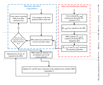
Figure 2: A flowchart illustrating the sequence, implementation and connections between the proposed learning scheme, matching algorithm and power allocation scheme.

V Simulation Results

In this section, we present simulation results and analysis to evaluate the performance of the proposed framework. For benchmarking, we consider the following baseline schemes:

1. HD-OMA scheme: users are associated to the nearest SBS and are allocated orthogonal resources for UL and DL. Requests are served using a round robin (RR) scheduler.

2. HD-NOMA only scheme: users are associated to the nearest SBS and RR scheduler is used to serve UL and DL queues. If there are multiple users in a scheduling queue, they are ranked according to their channel gains, and are served using NOMA if the ratio between their channel gains is at least $2$, otherwise, OMA is used. Power is allocated to NOMA users based on their channel ranking, in uniform descending order for UL NOMA and uniform ascending order for DL NOMA. SBSs operate either in UL or in DL depending on the queue length on each link direction.

3. FD-OMA scheme: users are associated to the nearest SBS and a pair of users is served in FD mode if the channel gain between them is greater than a certain threshold, otherwise users are served in HD mode using RR scheduler.

4. Uncoordinated scheme: in this scheme, users can be served in either HD or FD and in OMA or NOMA modes. The proposed matching algorithm, with inter-cell interference learning, is used for mode selection and user association. Power is assumed to be fixed for OMA and is similar to that of baseline $2$ for NOMA. This baseline represents an uncoordinated version of the proposed scheme.

V-A Simulation setup

We consider an outdoor cellular network where SBSs are distributed uniformly over the network area and users are distributed uniformly within small cells area. An SBS is located at the center of each small cell. SBS operate in TDD HD or in FD. If HD is used, they can operate in NOMA or OMA to serve multiple users. A packet-level simulator is considered and each experiment is run for $4000$ time subframes, which are sufficient for the traffic and virtual queues to get stable. Each result is averaged over $30$ different network topologies. The main simulation parameters are presented in Table II.

Table II: Simulation parameters

Parameter	Value
System bandwidth	10 MHz
Duplex modes	TDD HD/ FD
Multiplexing mode	OMA/NOMA
Sub-frame duration	1 ms
Network size	$500\times 500\>m^{2}$
Small cell radius	$40m$
Max. SBS transmit power	$22$ dBm
Max. user transmit power	$20$ dBm
Path loss model	Multi-cell pico scenario [35]
Shadowing standard deviation	$4$ dB
Penetration loss	$0$ dB
SI cancellation capability	$110$ dB
Max. quota of NOMA users $q$	$5$
Lyapunov parameters
$v$ parameter	$5\times 10^{7}$
UL power threshold $\delta_{u}^{\text{UL}}$	$0.5\times P_{\max}^{\text{UL}}$
DL power threshold $\delta_{b}^{\text{DL}}$	$0.9\times P_{\max}^{\text{DL}}$
Learning parameters
SBS learning parameter $\nu_{1}$	$0.1$
User learning parameter $\nu_{2}$	$0.1$

V-B Performance under different traffic intensity conditions

We start by evaluating the performance of the proposed scheme under different traffic intensity conditions. An average of $10$ users per SBS are distributed within the small cell area, with a user mean packet arrival rate $\lambda_{u}^{\text{total}}=\lambda_{u}^{\text{UL}}+\lambda_{u}^{\text{DL}}$, and $\lambda_{u}^{l}=5$ packet/s. Traffic intensity is varied by changing the mean packet size $1/\mu_{u}^{l}$ between $50$ kb and $400$ kb. In Figure 3, the packet throughput performance is depicted for the different schemes. The packet throughput is defined as the packet size successfully transmitted to the user divided by the delay encountered to complete its transmission. In moderate traffic conditions, the packet throughput increases with increasing traffic intensity, as the packet size increases and not much queuing delay is encountered. As the traffic intensity increases, queuing delay increases, correspondingly decreasing the packet throughput. Figure 3 shows that the proposed scheme outperforms the baseline schemes in packet throughput performance. At higher traffic intensity condition, gains of up to $63\%$ and $73\%$ are observed over HD-NOMA and FD-OMA baseline schemes, respectively. The performance of the uncoordinated scheme with matching is close to the proposed scheme at low traffic conditions. However, as the traffic load increases, the coordination gain reaches up to $31\%$.

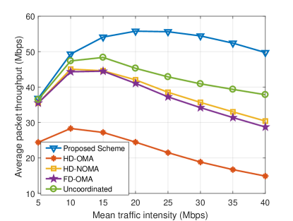
Figure 3: Average packet throughput performance for different schemes as the traffic intensity increases, for a network of $10$ SBSs and an average of $10$ UEs per SBS.

We continue by investigating the effect of traffic intensity on SBS mode selection. To that end, Figure 4 provides the ratio of transmissions carried out in FD or NOMA with respect to all transmissions in different traffic intensity conditions. Notice here that, although not explicitly represented, HD-OMA was the operation mode for the remaining of the transmissions.

The results show an increasing rate of operation in both FD and NOMA as the traffic intensity increases. The use of FD varies from about $3\%$ at low traffic conditions to $13\%$ at high traffic intensity, whereas NOMA operation accounts for up to $10\%$ of the transmissions under high traffic intensity conditions. The rest of transmissions are in HD-OMA mode. These results clearly indicate that an SBS can benefit more from scheduling multiple users simultaneously as traffic intensifies. This is mainly due to the higher request diversity, in which the chances to have subsets of users that benefit from being served simultaneously increase.

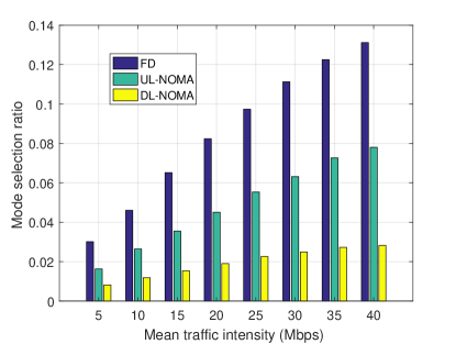
Figure 4: FD and NOMA mode selection ratios at different traffic intensity levels, for a network of $10$ SBSs and an average of $10$ UEs per SBS. Remaining transmissions are in HD-OMA mode.

Next, the impact of traffic intensity on UL/DL user rate throughput performance is analyzed through Figure 5. A close up look into Figure 5(a) and Figure 5(b) shows that results from all baseline schemes fall below HD-OMA for UL whereas for the DL this scheme is outperformed.

The DL-to-UL interference has a significant impact in the uncoordinated schemes due to the higher transmitting power of SBSs and lower pathloss between the SBS and user. In the DL case, the UL-to-DL interference can be partly avoided within each cell by the pairing thresholds used in the FD-OMA and HD-NOMA baselines. As our proposed scheme optimizes the UL and DL power allocation, it achieves UL and DL gains of $9\%$ and $23\%$ over the HD scheme, and of about $12\%$ in both UL and DL over the HD-NOMA and FD-OMA baseline schemes. Moreover, the coordination gain over the FD-NOMA matching scheme is even more evident in the UL ($12\%$) as compared to the DL ($7\%$), which is due to the dominance of DL-to-UL interference in the uncoordinated scenarios.

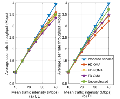
Figure 5: Average (a) UL and (b) DL rate throughput performance for different schemes as the network traffic intensity increases, for a network of $10$ SBSs and an average of $10$ UEs per SBS.

To further analyze the data rate throughput performance in the UL and DL, the cumulative distribution functions (CDFs) of the UL and DL user rate throughput for light and heavy traffic intensity cases are provided in Figure 6. As expected, in the presence of light traffic no significant gains are achieved with respect to HD scheme performance; Light traffic does not enable enough diversity for user scheduling purposes. Accordingly, most of the transmissions are in HD mode, as was also shown in Figure 4 for the proposed scheme. Under heavy traffic conditions, the baseline schemes suffer a degraded cell-edge throughput in the UL due to the DL-to-UL interference, as discussed above. Figure 6 also shows that the proposed scheme power optimization overcomes the cell-edge throughput degradation and achieves gains of at least $21\%$ and $17\%$ in the UL and DL $10$-th percentile throughput.

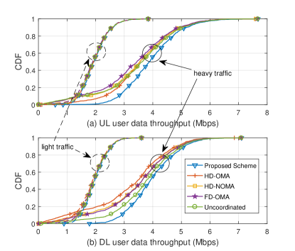
Figure 6: CDFs of UL and DL user throughput at light ($20$ Mbps) and heavy ($40$ Mbps) traffic intensity cases for a network of $10$ SBSs and an average of $10$ UEs per SBS.

V-C Performance under different network densities

We proceed by evaluating the performance of our proposed scheme as the network density increases. Different network densities will be simulated by introducing an increased number of SBSs in the system, while intra-cell user density and traffic influx rates are kept constant. First, we compare the packet throughput performance against the baseline schemes. Figure 7 shows that, at low network density, all schemes achieve almost double the packet throughput of the HD baseline scheme. This is due to multiplexing gain where SBSs are able to serve more than one user simultaneously and with not much inter-cell interference to affect the performance. For the same reason, the uncoordinated scheme performance is close to the proposed scheme, since coordinating the power to avoid inter-cell interference is not crucial in this case. On the other hand, as the network density increases, the coordination gain increases, reaching up to $55\%$ for $14$ SBSs.

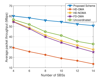
Figure 7: Average packet throughput performance for different schemes as the network density increases for an average of $10$ UEs per SBS and a mean traffic intensity of $3$ Mbps per user.

Next, we investigate the ratio of selecting FD and NOMA modes in the proposed schemes as the network density varies. As Figure 8 shows, as the network density increases, the selection of DL NOMA decreases. The decrease is due to the way power is allocated in DL NOMA, where users with less channel gains (typically cell-edge users) have to be allocated higher power as compared to users with higher channel gains. In that case, user with higher channel gains can decode and cancel others’ data before decoding their own. Therefore, as the network density increases, inter-cell interference levels increase, making it is less likely to benefit from DL NOMA. Instead, SBSs schedule DL users either in HD-OMA or FD modes.

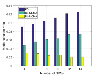
Figure 8: FD and NOMA mode selection ratios as the network density increases for an average of $10$ UEs per SBS and a mean traffic intensity of $3$ Mbps per user. Remaining transmissions are in HD-OMA mode.

V-D Impact of SI cancellation capability

Finally, in this subsection, the effect of the SBS SI cancellation capability on the proposed and baseline schemes is analyzed. Figure 9 compares the average packet throughput performance of the different schemes as the SI cancellation varies from $30$ dB to $110$ dB, which is the highest reported capability level. As Figure 9 shows, the degradation in the proposed scheme performance due to having lower SI cancellation levels is minor compared to the FD-OMA baseline scheme. As the proposed scheme optimizes the mode selection, it can operate more frequently in UL NOMA instead of FD to serve UL users, so that the high interference from the SBS DL signal is avoided.

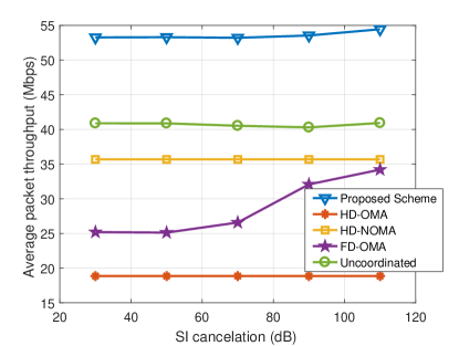
Figure 9: Average packet throughput performance for different schemes as the SBS SI cancellation capability varies, for a network of $10$ SBSs, an average of $10$ UEs per SBS, and a mean traffic intensity rate of $3$ Mbps per user.

Figure 10 shows the selection ratio of FD and NOMA modes in the proposed scheme at different SI cancellation levels. It can be seen that FD mode is selected more frequently at higher SI cancellation levels, whereas the UL NOMA ratio decreases correspondingly. The ratio of DL NOMA selection maintains the same, since SI interference only affects the UL transmissions.

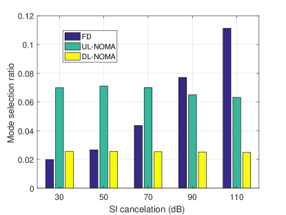
Figure 10: FD and NOMA mode selection ratios at different SBS SI cancellation capability levels, for a network of $10$ SBSs, an average of $10$ UEs per SBS, and a mean traffic intensity rate of $3$ Mbps per user. Remaining transmissions are in HD-OMA mode.

VI Conclusions

In this paper, the problem of mode selection, dynamic user association, and power optimization has been studied for IBFD and NOMA operating networks. The problem of time-averaged UL and DL rate maximization problem under queue stability constraints has been formulated and solved using Lyapunov framework. A many-to-one matching algorithm is proposed that locally select which users to serve and in which transmission mode to operate. Then, a power optimization problem of the matched users has been formulated and solved iteratively. Simulations results show significant gains of up to $63\%$ and $73\%$ in UL and DL packet throughput, and $21\%$ and $17\%$ in UL and DL cell edge throughput, respectively. Possible future research directions are to study the problem in ultra-dense network environments as well as optimizing the network for latency and reliability requirements.

Mohammed S. Elbamby received his B.Sc. degree (honors) in electronics and communications engineering from the Institute of Aviation Engineering and Technology (IAET), Egypt, in 2010, and his M.Sc. degree in Communications engineering from Cairo University, Egypt, in 2013. After receiving his M.Sc. degree, he joined the Centre for Wireless Communications (CWC) at the University of Oulu, where he is working toward his doctoral degree. His research interests include resource optimization, UL/DL configuration, fog networking, and caching in wireless cellular networks. Mohammed S. Elbamby is a recipient of the Best Student Paper Award from the European Conference on Networks and Communications (EuCNC’2017).

Mehdi Bennis (Senior Member, IEEE) received his M.Sc. degree in Electrical Engineering jointly from the EPFL, Switzerland and the Eurecom Institute, France in 2002. From 2002 to 2004, he worked as a research engineer at IMRA-EUROPE investigating adaptive equalization algorithms for mobile digital TV. In 2004, he joined the Centre for Wireless Communications (CWC) at the University of Oulu, Finland as a research scientist. In 2008, he was a visiting researcher at the Alcatel-Lucent chair on flexible radio, SUPELEC. He obtained his Ph.D. in December 2009 on spectrum sharing for future mobile cellular systems. Currently Dr. Bennis is an Adjunct Professor at the University of Oulu and Academy of Finland research fellow. His main research interests are in radio resource management, heterogeneous networks, game theory and machine learning in 5G networks and beyond. He has co-authored one book and published more than 100 research papers in international conferences, journals and book chapters. He was the recipient of the prestigious 2015 Fred W. Ellersick Prize from the IEEE Communications Society, the 2016 Best Tutorial Prize from the IEEE Communications Society and the 2017 EURASIP Best paper Award for the Journal of Wireless Communications and Networks. Dr. Bennis serves as an editor for the IEEE Transactions on Wireless Communication.

Walid Saad (S’07, M’10, SM 15) received his Ph.D degree from the University of Oslo in 2010. Currently, he is an Associate Professor at the Department of Electrical and Computer Engineering at Virginia Tech, where he leads the Network Science, Wireless, and Security (NetSciWiS) laboratory, within the Wireless@VT research group. His research interests include wireless networks, game theory, cybersecurity, unmanned aerial vehicles, and cyber-physical systems. Dr. Saad is the recipient of the NSF CAREER award in 2013, the AFOSR summer faculty fellowship in 2014, and the Young Investigator Award from the Office of Naval Research (ONR) in 2015. He was the author/co-author of five conference best paper awards at WiOpt in 2009, ICIMP in 2010, IEEE WCNC in 2012, IEEE PIMRC in 2015, and IEEE SmartGridComm in 2015. He is the recipient of the 2015 Fred W. Ellersick Prize from the IEEE Communications Society. In 2017, Dr. Saad was named College of Engineering Faculty Fellow at Virginia Tech. From 2015 2017, Dr. Saad was named the Steven O. Lane Junior Faculty Fellow at Virginia Tech. He currently serves as an editor for the IEEE Transactions on Wireless Communications, IEEE Transactions on Communications, and IEEE Transactions on Information Forensics and Security.

M rouane Debbah entered the Ecole Normale Sup rieure Paris-Saclay (France) in 1996 where he received his M.Sc and Ph.D. degrees respectively. He worked for Motorola Labs (Saclay, France) from 1999-2002 and the Vienna Research Center for Telecommunications (Vienna, Austria) until 2003. From 2003 to 2007, he joined the Mobile Communications department of the Institut Eurecom (Sophia Antipolis, France) as an Assistant Professor. Since 2007, he is a Full Professor at CentraleSupelec (Gif-sur-Yvette, France). From 2007 to 2014, he was the director of the Alcatel-Lucent Chair on Flexible Radio. Since 2014, he is Vice-President of the Huawei France R&D center and director of the Mathematical and Algorithmic Sciences Lab. His research interests lie in fundamental mathematics, algorithms, statistics, information & communication sciences research. He is an Associate Editor in Chief of the journal Random Matrix: Theory and Applications and was an associate and senior area editor for IEEE Transactions on Signal Processing respectively in 2011-2013 and 2013-2014. M rouane Debbah is a recipient of the ERC grant MORE (Advanced Mathematical Tools for Complex Network Engineering). He is a IEEE Fellow, a WWRF Fellow and a member of the academic senate of Paris-Saclay. He has managed 8 EU projects and more than 24 national and international projects. He received 17 best paper awards, among which the 2007 IEEE GLOBECOM best paper award, the Wi-Opt 2009 best paper award, the 2010 Newcom++ best paper award, the WUN CogCom Best Paper 2012 and 2013 Award, the 2014 WCNC best paper award, the 2015 ICC best paper award, the 2015 IEEE Communications Society Leonard G. Abraham Prize, the 2015 IEEE Communications Society Fred W. Ellersick Prize, the 2016 IEEE Communications Society Best Tutorial paper award, the 2016 European Wireless Best Paper Award and the 2017 Eurasip Best Paper Award as well as the Valuetools 2007, Valuetools 2008, CrownCom2009, Valuetools 2012 and SAM 2014 best student paper awards. He is the recipient of the Mario Boella award in 2005, the IEEE Glavieux Prize Award in 2011 and the Qualcomm Innovation Prize Award in 2012.

Matti Latva-aho received the M.Sc., Lic.Tech. and Dr. Tech (Hons.) degrees in Electrical Engineering from the University of Oulu, Finland in 1992, 1996 and 1998, respectively. From 1992 to 1993, he was a Research Engineer at Nokia Mobile Phones, Oulu, Finland after which he joined Centre for Wireless Communications (CWC) at the University of Oulu. Prof. Latva-aho was Director of CWC during the years 1998-2006 and Head of Department for Communication Engineering until August 2014. Currently he is Professor of Digital Transmission Techniques at the University of Oulu. He serves as Academy of Finland Professor in 2017 - 2022. His research interests are related to mobile broadband communication systems and currently his group focuses on 5G systems research. Prof. Latva-aho has published 300+ conference or journal papers in the field of wireless communications. He received Nokia Foundation Award in 2015 for his achievements in mobile communications research.

References

- [1] Q. C. Li, H. Niu, A. T. Papathanassiou, and G. Wu, “5G network capacity: Key elements and technologies,” IEEE Vehicular Technology Magazine, vol. 9, pp. 71–78, March 2014.
- [2] M. Duarte and A. Sabharwal, “Full-duplex wireless communications using off-the-shelf radios: Feasibility and first results,” in 2010 Conference Record of the Forty Fourth Asilomar Conference on Signals, Systems and Computers, pp. 1558–1562, Nov 2010.
- [3] M. Jain, J. I. Choi, T. Kim, D. Bharadia, S. Seth, K. Srinivasan, P. Levis, S. Katti, and P. Sinha, “Practical, real-time, full duplex wireless,” in Proceedings of the 17th Annual International Conference on Mobile Computing and Networking, MobiCom ’11, (New York, NY, USA), pp. 301–312, 2011.
- [4] H. Thomsen, P. Popovski, E. d. Carvalho, N. K. Pratas, D. M. Kim, and F. Boccardi, “CoMPflex: CoMP for in-band wireless full duplex,” IEEE Wireless Communications Letters, vol. 5, pp. 144–147, April 2016.
- [5] H. Alves, C. H. M. de Lima, P. H. J. Nardelli, R. D. Souza, and M. Latva-aho, “On the average spectral efficiency of interference-limited full-duplex networks,” in 2014 9th International Conference on Cognitive Radio Oriented Wireless Networks and Communications (CROWNCOM), pp. 550–554, June 2014.
- [6] J. Lee and T. Q. S. Quek, “Hybrid full-/half-duplex system analysis in heterogeneous wireless networks,” IEEE Transactions on Wireless Communications, vol. 14, pp. 2883–2895, May 2015.
- [7] M. Gatnau, G. Berardinelli, N. H. Mahmood, and P. Mogensen, “Can full duplex boost throughput and delay of 5G ultra-dense small cell networks?,” in 2016 IEEE 83st Vehicular Technology Conference (VTC Spring), pp. 1–5, May 2016.
- [8] Y. Saito, Y. Kishiyama, A. Benjebbour, T. Nakamura, A. Li, and K. Higuchi, “Non-orthogonal multiple access (NOMA) for cellular future radio access,” in Vehicular Technology Conference (VTC Spring), 2013 IEEE 77th, pp. 1–5, June 2013.
- [9] Z. Wei, J. Yuan, D. W. K. Ng, M. Elkashlan, and Z. Ding, “A survey of downlink non-orthogonal multiple access for 5G wireless communication networks,” CoRR, vol. abs/1609.01856, 2016.
- [10] T. Takeda and K. Higuchi, “Enhanced user fairness using non-orthogonal access with SIC in cellular uplink,” in Vehicular Technology Conference (VTC Fall), 2011 IEEE, pp. 1–5, Sept 2011.
- [11] S. Goyal, P. Liu, S. Panwar, R. A. DiFazio, R. Yang, J. Li, and E. Bala, “Improving small cell capacity with common-carrier full duplex radios,” in 2014 IEEE International Conference on Communications (ICC), pp. 4987–4993, June 2014.
- [12] J. M. B. da Silva, Y. Xu, G. Fodor, and C. Fischione, “Distributed spectral efficiency maximization in full-duplex cellular networks,” in 2016 IEEE International Conference on Communications Workshops (ICC), pp. 80–86, May 2016.
- [13] P. Tehrani, F. Lahouti, and M. Zorzi, “Resource allocation in OFDMA networks with half-duplex and imperfect full-duplex users,” CoRR, vol. abs/1605.01947, 2016.
- [14] B. Di, S. Bayat, L. Song, and Y. Li, “Radio resource allocation for downlink non-orthogonal multiple access (NOMA) networks using matching theory,” in 2015 IEEE Global Communications Conference (GLOBECOM), pp. 1–6, Dec 2015.
- [15] P. Parida and S. S. Das, “Power allocation in OFDM based NOMA systems: A DC programming approach,” in 2014 IEEE Globecom Workshops (GC Wkshps), pp. 1026–1031, Dec 2014.
- [16] F. Fang, H. Zhang, J. Cheng, and V. C. M. Leung, “Energy-efficient resource allocation for downlink non-orthogonal multiple access network,” IEEE Transactions on Communications, vol. 64, pp. 3722–3732, Sept 2016.
- [17] M. Al-Imari, P. Xiao, M. A. Imran, and R. Tafazolli, “Uplink non-orthogonal multiple access for 5G wireless networks,” in 2014 11th International Symposium on Wireless Communications Systems (ISWCS), pp. 781–785, Aug 2014.
- [18] S. Goyal, P. Liu, and S. Panwar, “User Selection and Power Allocation in Full Duplex Multi-Cell Networks,” ArXiv e-prints arXiv:1604.08937, Apr. 2016.
- [19] R. Sultan, L. Song, K. G. Seddik, Y. Li, and Z. Han, “Mode selection, user pairing, subcarrier allocation and power control in full-duplex OFDMA HetNets,” in 2015 IEEE International Conference on Communication Workshop (ICCW), pp. 210–215, June 2015.
- [20] B. Di, S. Bayat, L. Song, and Y. Li, “Radio resource allocation for full-duplex OFDMA networks using matching theory,” in Computer Communications Workshops (INFOCOM WKSHPS), 2014 IEEE Conference on, pp. 197–198, April 2014.
- [21] I. Atzeni, M. Kountouris, and G. C. Alexandropoulos, “Performance evaluation of user scheduling for full-duplex small cells in ultra-dense networks,” CoRR, vol. abs/1604.05979, 2016.
- [22] M. S. Ali, H. Tabassum, and E. Hossain, “Dynamic user clustering and power allocation for uplink and downlink non-orthogonal multiple access (NOMA) systems,” IEEE Access, vol. PP, no. 99, pp. 1–1, 2016.
- [23] S. Sekander, H. Tabassum, and E. Hossain, “Decoupled uplink-downlink user association in multi-tier full-duplex cellular networks: A two-sided matching game,” IEEE Transactions on Mobile Computing, vol. PP, no. 99, pp. 1–1, 2016.
- [24] Y. Sun, D. W. K. Ng, Z. Ding, and R. Schober, “Optimal joint power and subcarrier allocation for full-duplex multicarrier non-orthogonal multiple access systems,” IEEE Transactions on Communications, vol. 65, pp. 1077–1091, March 2017.
- [25] B. Di, L. Song, and Y. Li, “Sub-channel assignment, power allocation and user scheduling for non-orthogonal multiple access networks,” CoRR, vol. abs/1608.08313, 2016.
- [26] A. Celik, R. M. Radaydeh, F. S. Al-Qahtani, A. H. A. El-Malek, and M.-S. Alouini, “Resource allocation and cluster formation for imperfect NOMA in DL/UL decoupled hetnets,” in IEEE Global Communications Conference (GLOBECOM), pp. 1–7, Dec 2017.
- [27] M. J. Neely, “A Lyapunov optimization approach to repeated stochastic games,” CoRR, vol. abs/1310.2648, 2013.
- [28] M. J. Neely, “Stochastic network optimization with application to communication and queueing systems,” Synthesis Lectures on Communication Networks, vol. 3, no. 1, pp. 1–211, 2010.
- [29] D. Gale and L. S. Shapley, “College admissions and the stability of marriage,” The American Mathematical Monthly, vol. 69, no. 1, pp. 9–15, 1962.
- [30] A. Roth and M. Sotomayor, “Two-sided matching: A study in game-theoretic modeling and analysis,” Cambridge University Press, Cambridge, 1992.
- [31] Y. Gu, W. Saad, M. Bennis, M. Debbah, and Z. Han, “Matching theory for future wireless networks: fundamentals and applications,” IEEE Communications Magazine, vol. 53, pp. 52–59, May 2015.
- [32] A. L. Yuille and A. Rangarajan, “The Concave-convex Procedure,” Neural Comput., vol. 15, pp. 915–936, Apr. 2003.
- [33] T. Lipp and S. Boyd, “Variations and extension of the convex–concave procedure,” Optimization and Engineering, vol. 17, no. 2, pp. 263–287, 2016.
- [34] S. Boyd and L. Vandenberghe, Convex Optimization. Cambridge University Press, 2009.
- [35] 3GPP, “Further Enhancements to LTE TDD for DL-UL Interference Management and Traffic Adaptation,” TR 36.828, 3rd Generation Partnership Project (3GPP), June 2012.