Frame multiplication theory and a vector-valued DFT and ambiguity function

Abstract.

Vector-valued discrete Fourier transforms (DFTs) and ambiguity functions are defined. The motivation for the definitions is to provide realistic modeling of multi-sensor environments in which a useful time-frequency analysis is essential. The definition of the DFT requires associated uncertainty principle inequalities. The definition of the ambiguity function requires a component that leads to formulating a mathematical theory in which two essential algebraic operations can be made compatible in a natural way. The theory is referred to as frame multiplication theory. These definitions, inequalities, and theory are interdependent, and they are the content of the paper with the centerpiece being frame multiplication theory.

The technology underlying frame multiplication theory is the theory of frames, short time Fourier transforms (STFTs), and the representation theory of finite groups. The main results have the following form: frame multiplication exists if and only if the finite frames that arise in the theory are of a certain type, e.g., harmonic frames, or, more generally, group frames.

In light of the complexities and the importance of the modeling of time-varying and dynamical systems in the context of effectively analyzing vector-valued multi-sensor environments, the theory of vector-valued DFTs and ambiguity functions must not only be mathematically meaningful, but it must have constructive implementable algorithms, and be computationally viable. This paper presents our vision for resolving these issues, in terms of a significant mathematical theory, and based on the goal of formulating and developing a useful vector-valued theory.

1. Introduction

1.1. Background

Our background for this work was based in the following program.

• Originally, our problem was to construct libraries of phase-coded waveforms $v:{\mathbb{R}}\longrightarrow{\mathbb{C}},$ parameterized by design variables, for use in communications and radar. A goal was to achieve diverse narrow-band ambiguity function behavior of $v$ by defining new classes of discrete quadratic phase and number theoretic perfect autocorrelation sequences $u:{\mathbb{Z}}/N{\mathbb{Z}}\longrightarrow{\mathbb{C}}$ with which to define $v$ and having optimal autocorrelation behavior in a way to be defined.

• Then, a realistic more general problem was to construct vector-valued waveforms $v$ in terms of vector-valued sequences $u:{\mathbb{Z}}/N{\mathbb{Z}}\longrightarrow{\mathbb{C}}^{d}$ having this optimal autocorrelation behavior. Such sequences are relevant in light of vector sensor capabilities and modeling, e.g., see [63], [77].

In fact, we shall define periodic vector-valued discrete Fourier transforms (DFTs) and narrow-band ambiguity functions. Early-on we understood that the accompanying theory could not just be a matter of using bold-faced letters to recount existing theory, an image used by Joel Tropp for another multi-dimensional situation. Two of us recorded our initial results on the subject at an invited talk at Asilomar (2008), [10], but we did not pursue it then, because there was the fundamental one-dimensional problem, mentioned above in the first bullet, that had to be resolved. Since then, we have made appropriate progress on this one-dimensional problem, see [14, 8, 7].

1.2. Goals and short time Fourier transform (STFT) theme

In 1953, P. M. Woodward [91, 90] defined the narrow-band radar ambiguity function. The narrow-band ambiguity function is a two-dimensional function of delay $t$ and Doppler frequency $\gamma$ that measures the correlation between a waveform $w$ and its Doppler distorted version. The information given by the narrow-band ambiguity function is important for practical purposes in radar. In fact, the waveform design problem is to construct waveforms having “good” ambiguity function behavior in the sense of being designed to solve real problems.

Since we are only dealing with narrow-band ambiguity functions, we shall suppress the words “narrow-band” for the remainder.

Definition 1.1 (Ambiguity function).

a. The ambiguity function $A(v)$ of $v\in L^{2}({\mathbb{R}})$ is

(1) $$A(v)(t,\gamma) =\int_{{\mathbb{R}}}v(s+t)\overline{v(s)}e^{-2\pi is\gamma}\,ds$$

$$=e^{\pi it\gamma}\int_{{\mathbb{R}}}v\left(s+\frac{t}{2}\right)\overline{v\left(s-\frac{t}{2}\right)}e^{-2\pi is\gamma}ds,$$

for $(t,\gamma)\in{\mathbb{R}}^{2}$.

b. We shall only be interested in the discrete version of (1). For an $N$-periodic function $u:{\mathbb{Z}}/N{\mathbb{Z}}\rightarrow{\mathbb{C}}$ the discrete periodic ambiguity function is

(2) $$A_{p}(u)(m,n)=\frac{1}{N}\sum_{k=0}^{N-1}u(m+k)\overline{u(k)}e^{-2\pi ikn/N},$$

for $(m,n)\in{\mathbb{Z}}/N{\mathbb{Z}}\times{\mathbb{Z}}/N{\mathbb{Z}}$.

c. If $v,w\in L^{2}({\mathbb{R}})$, the cross-ambiguity function $A(v,w)$ of $v$ and $w$ is

$$A(v,w)(t,\gamma) =\int_{{\mathbb{R}}}v(s+t)\overline{w(s)}e^{-2\pi is\gamma}\,ds$$

(3) $$=e^{2\pi it\gamma}\int_{{\mathbb{R}}}v(s)\overline{w(s-t)}e^{-2\pi is\gamma}\,ds.$$

Evidently, $A(v)=A(v,v)$, so that the ambiguity function is a special case of the cross-ambiguity function.

d. The short-time Fourier transform (STFT) of $v$ with respect to a window function $w\in L^{2}({\mathbb{R}})\setminus\{0\}$ is

(4) $$V_{w}(v)(t,\gamma)=\int_{{\mathbb{R}}}v(s)\overline{w(s-t)}e^{-2\pi is\gamma}\,ds$$

for $(t,\gamma)\in{\mathbb{R}}^{2},$ see [47] for a definitive mathematical treatment. Thus, we think of the window $w$ as centered at $t$, and we have

(5) $$A(v,w)(t,\gamma)=e^{2\pi it\gamma}\,V_{w}(v)(t,\gamma).$$

e. $A(v,w)$ and $V_{w}(v)$ can clearly be defined for functions $v,w$ on ${\mathbb{R}}^{d}$ and for other function spaces besides $L^{2}({\mathbb{R}}^{d}).$ The quantity $|V_{w}(v)|$ is the spectrogram of $v,$ that is so important in power spectrum analysis, see, e.g., [89], [17], [68], [70], [24], [65], [83].

Our goals are the following.

• Ultimately, we shall establish the theory of vector-valued ambiguity functions of vector-valued functions $v$ on ${\mathbb{R}}^{d}$ in terms of their discrete periodic counterparts on ${\mathbb{Z}}/N{\mathbb{Z}}.$

• To this end, in this paper, we define vector-valued DFTs and discrete periodic vector-valued ambiguity functions on ${\mathbb{Z}}/N{\mathbb{Z}}$ in a natural way.

The STFT is the guide and the theory of frames, especially the theory of DFT, harmonic, and group frames, is the framework (sic) to formulate these goals. The underlying technology that allows us to obtain these goals is frame multiplication theory.

1.3. Outline

We begin with an extended exposition on the theory of frames (Section 2). The reason is that frames are essential for our results, and our results are sometimes not conceived in terms of frames. As such, it made sense to add sufficient background material.

The vector-valued discrete Fourier transform (DFT) is developed in Subsection 3.1. The remaining two subsections of Section 3 conclude with a comparison of relations between Subsection 3.1 and apparently different implications from the Gelfand theory. Subsection 3.1 is required in our vector-valued ambiguity function theory.

Section 4 establishes the basic role of the STFT in achieving the goals listed in Subsection 1.2. In the process, we formulate our idea leading to the notion of frame multiplication, that is used to define the vector-valued ambiguity function. In Section 4 we also give two diverse examples. The first is for DFT frames (Subsection 4.2), that we present in an Abelian setting. The second is for cross-product frames (Subsection 4.4), that is fundamentally non-Abelian and non-group with regard to structure, and that is motivated by the recent applicability of quaternions, e.g., [61]. Subsection 4.3 relates the examples of Subsections 4.2 and 4.4, and formally motivates the theory of frame multiplication presented in Section 5.

In Section 6 we define the harmonic and group frames that are the basis for our Abelian group frame multiplication results of Section 7. Although we present the results in the setting of finite Abelian groups and $d$-dimensional Hilbert spaces, many of them can be generalized; and, in fact, some are more easily formulated and proved in the general setting. As such, some of the theory in these sections is given in infinite and/or non-Abelian terms. The major results are stated and proved in Subsection 7.2. They characterize the existence of frame multiplication in term of harmonic and group frames.

Section 8.2 is devoted to the uncertainty principle in the context of our vector-valued DFT theory.

We close with Appendix 9. Some of this material is used explicitly in Sections 6 and 7, and some provides a theoretical umbrella to cover the theory herein and the transition to the non-Abelian case beginning with [2].

Remark 1.2.

The forthcoming non-Abelian theory is due to Travis Andrews [2]. In fact, if $(G,\bullet)$ is a finite group with representation $\rho:G\rightarrow GL({\mathbb{C}}^{d})$, then we can show that there is a frame $\{x_{n}\}_{n\in G}$ and bilinear multiplication, $\ast:{\mathbb{C}}^{d}\times{\mathbb{C}}^{d}\rightarrow{\mathbb{C}}^{d}$, such that $x_{m}\ast x_{n}=x_{m\bullet n}$.

Further, we are extending the theory to tight frames for finite dimensional Hilbert spaces $H$ over ${\mathbb{C}}$ and finite rings $G$, so that there are meaningful generalizations of the vector-valued $A_{p}^{d}(u)$ theory in the formal but motivated settings of Equations (20) and (21).

It remains to establish the theory in infinite dimensional Hilbert spaces and associated infinite locally compact groups and rings as well as tantalizing non-group cases, see, e.g., our cross product example in Subsection 4.4 and its relationship to quaternion groups.

2. Frames

2.1. Definitions and properties

Frames are a generalization of orthonormal bases where we relax Parseval’s identity to allow for overcompleteness. Frames were first introduced in 1952 by Duffin and Schaeffer [34] and have become the subject of intense study since the 1980s. e.g., see [29], [16], [5], [25], [22]. (In fact, Paley and Wiener gave the technical definition of a frame in [67], but they only developed the completeness properties.)

Definition 2.1 (Frame).

a. Let $H$ be a separable Hilbert space over the field ${\mathbb{F}},$ where ${\mathbb{F}}={\mathbb{R}}$ or ${\mathbb{F}}={\mathbb{C}}.$ A finite or countably infinite sequence, $X=\{x_{j}\}_{j\in J},$ of elements of $H$ is a frame for $H$ if

(6) $$\exists A,B>0\;\text{such that}\;\forall x\in H,\quad A\left\|x\right\|^{2}\leq\sum_{j\in J}|\langle{x},{x_{j}}\rangle|^{2}\leq B\left\|x\right\|^{2}.$$

The optimal constants, viz., the supremum over all such $A$ and infimum over all such $B$, are called the lower and upper frame bounds respectively. When we refer to frame bounds $A$ and $B$, we shall mean these optimal constants.

b. A frame $X$ for $H$ is a tight frame if $A=B.$ If a tight frame has the further property that $A=B=1,$ then the frame is a Parseval frame for $H.$

c. A frame $X$ for $H$ is equal-norm if each of the elements of $X$ has the same norm. Further, a frame $X$ for $H$ is a unit norm tight frame (UNTF) if each of the elements of $X$ has norm $1.$ If $H$ is finite dimensional and $X$ is an UNTF for $H,$ then $X$ is a finite unit norm tight frame (FUNTF).

d. A sequence of elements of $H$ satisfying an upper frame bound, such as $B\left\|x\right\|^{2}$ in (6), is a Bessel sequence.

Remark 2.2.

The series in (6) is an absolutely convergent series of positive numbers; and so, any reordering of the sequence of frame elements or reindexing by another set of the same cardinality will remain a frame. We allow for repetitions of vectors in a frame so that, strictly speaking, the set of vectors, that we also call $X$, is a multi-set. We shall index frames by an arbitrary sequence such as $J$ in the definition, or by specific sequences such as the set ${\mathbb{N}}$ of positive integers or the set ${\mathbb{Z}}^{d},d\geq 2,$ of multi-integers when it is natural to do so.

Let $X=\{x_{j}\}_{j\in J}$ be a frame for $H$. We define the following operators associated with every frame; they are crucial to frame theory and will be used extensively. The analysis operator $L:H\rightarrow\ell^{2}(J)$ is defined by

$$\forall x\in H,\quad Lx=\{\langle{x,x_{j}}\rangle\}_{j\in J}.$$

Inequality $\eqref{eq:framedef}$ ensures that the analysis operator $L$ is bounded. If $H_{1}$ and $H_{2}$ are separable Hilbert spaces and if $T:H_{1}\rightarrow H_{2}$ is a linear operator, then the operator norm $\left\|T\right\|_{op}$ of $T$ is

$$\left\|T\right\|_{op}={\rm sup}_{\left\|x\right\|_{H_{1}}\leq 1}\left\|T(x)\right\|_{H_{2}}.$$

Clearly, we have $\left\|L\right\|_{op}\leq\sqrt{B}$. The adjoint of the analysis operator is the synthesis operator $L^{\ast}:\ell^{2}(J)\rightarrow H$, and it is defined by

$$\forall a\in\ell^{2}(J),\quad L^{\ast}a=\sum_{j\in J}a_{j}x_{j}.$$

From Hilbert space theory, we know that any bounded linear operator $T:H\rightarrow H$ satisfies $\left\|T\right\|_{op}=\left\|T^{\ast}\right\|_{op}.$ Therefore, the synthesis operator $L^{\ast}$ is bounded and $\left\|L^{\ast}\right\|_{op}\leq\sqrt{B}$.

The frame operator is the mapping $S:H\rightarrow H$ defined as $S=L^{\ast}L$, i.e.,

$$\forall x\in H,\quad Sx=\sum_{j\in J}\langle{x,x_{j}}\rangle x_{j}.$$

We shall describe $S$ more fully. First, we have that

$$\forall x\in H,\quad\langle{Sx,x}\rangle=\sum_{j\in J}\left|\langle{x,x_{j}}\rangle\right|^{2}.$$

Thus, $S$ is a positive and self-adjoint operator, and $\eqref{eq:framedef}$ can be rewritten as

$$\forall x\in H,\quad A\left\|x\right\|^{2}\leq\langle{Sx,x}\rangle\leq B\left\|x\right\|^{2},$$

or, more compactly, as

$$AI\leq S\leq BI.$$

It follows that $S$ is invertible ([29], [5]), $S$ is a multiple of the identity precisely when $X$ is a tight frame, and

(7) $$B^{-1}I\leq S^{-1}\leq A^{-1}I.$$

Hence, $S^{-1}$ is a positive self-adjoint operator and has a square root $S^{-1/2}$ (Theorem 12.33 in [74]). This square root can be written as a power series in $S^{-1}$; consequently, it commutes with every operator that commutes with $S^{-1},$ and, in particular, with $S.$ Utilizing these facts we can prove a theorem that tells us that frames share an important property with orthonormal bases, viz., there is a reconstruction formula.

Theorem 2.3 (Frame reconstruction formula).

Let $H$ be a separable Hilbert space, and let $X=\{x_{j}\}_{j\in J}$ be a frame for $H$ with frame operator $S$. Then

$$\forall x\in H,\quad x=\sum_{j\in J}\langle{x,x_{j}}\rangle S^{-1}x_{j}=\sum_{j\in J}\langle{x,S^{-1}x_{j}}\rangle x_{j}=\sum_{j\in J}\langle{x,S^{-1/2}x_{j}}\rangle S^{-1/2}x_{j},$$

where the mapping $S:H\rightarrow H,$ $x\mapsto\sum_{j\in J}\langle{x,x_{j}}\rangle x_{j},$ is a well-defined topological isomorphism.

Proof.

The proof is three computations. From $I=S^{-1}S$, we have

$$\forall x\in H,\quad x=S^{-1}Sx=S^{-1}\sum_{j\in J}\langle{x,x_{j}}\rangle x_{j}=\sum_{j\in J}\langle{x,x_{j}}\rangle S^{-1}x_{j};$$

from $I=SS^{-1}$, we have

$$\forall x\in H,\quad x=SS^{-1}x=\sum_{j\in J}\langle{S^{-1}x,x_{j}}\rangle x_{j}=\sum_{j\in J}\langle{x,S^{-1}x_{j}}\rangle x_{j};$$

and from $I=S^{-1/2}SS^{-1/2}$, it follows that

$$\forall x\in H,\,x=S^{-1/2}SS^{-1/2}x=S^{-1/2}\sum_{j\in J}\langle{S^{-1/2}x,x_{j}}\rangle x_{j}=\sum_{j\in J}\langle{x,S^{-1/2}x_{j}}\rangle S^{-1/2}x_{j}.\qed$$

From the frame reconstruction formula and (7), it follows that $\{S^{-1}x_{j}\}_{j\in J}$ is a frame with frame bounds $B^{-1}$ and $A^{-1}$ and $\{S^{-1/2}x_{j}\}_{j\in J}$ is a Parseval frame.

Definition 2.4 (Canonical dual).

Let $X=\{x_{j}\}_{j\in J}$ be a frame for a separable Hilbert space $H$ with frame operator $S$. The frame $S^{-1}X=\{S^{-1}x_{j}\}_{j\in J}$ is the canonical dual frame of $X$. The frame $S^{-1/2}X=\{S^{-1/2}x_{j}\}_{j\in J}$ is the canonical tight frame of $X$.

The Gramian operator is the mapping $G:\ell^{2}(J)\rightarrow\ell^{2}(J)$ defined as $G=LL^{\ast}$. If $\{x_{j}\}_{j\in J}$ is the standard orthonormal basis for $\ell^{2}(J)$, then

(8) $$\forall a=\{a_{j}\}_{j\in J}\in\ell^{2}(J),\quad\langle{Ga,x_{k}}\rangle=\sum_{j\in J}a_{j}\langle{x_{j},x_{k}}\rangle.$$

2.2. FUNTFs

We shall often deal with FUNTFs $X=\{x_{j}\}_{j=1}^{N}$ for ${\mathbb{C}}^{d}.$

The most interesting setting is for the case when $N>d.$ In fact, frames can provide redundant signal representation to compensate for hardware errors, can ensure numerical stability, and are a natural model for minimizing the effects of noise. Particular areas of a recent applicability of FUNTFs include the following topics:

• Robust transmission of data over erasure channels such as the internet, e.g., see [46], [44], [21];

• Multiple antenna code design for wireless communications, e.g., see [56];

• Multiple description coding, e.g., see [45], [78];

• Quantum detection, e.g., see [40], [18], [12];

• Grassmannian “min-max” waveforms, e.g., see [20], [78], [13].

The following is a consequence of (6).

Theorem 2.5.

If $X=\{x_{j}\}_{j=0}^{N-1}$ is a FUNTF for ${\mathbb{F}}^{d}$, then

$$\forall x\in{\mathbb{F}}^{d},\quad x=\frac{d}{N}\sum_{j=0}^{N-1}\langle x,x_{j}\rangle x_{j}.$$

Remark 2.6.

It is important to understand the geometry of FUNTFs. e.g., at the most elementary level, the vertices of the Platonic solids centered at the origin are FUNTFs. Further, FUNTFs can be characterized as the minima of a potential energy function, see [11] for the details of this result.

Orthonormal bases for $H={\mathbb{F}}^{d}$ are both Parseval frames and FUNTFs. If $X=\{x_{j}\}_{j=0}^{N-1}$ is Parseval for $H$ and each $\|x_{j}\|=1,$ then $N=d$ and $X$ is an ONB for $H$. If $X$ is a FUNTF with frame constant $A,$ then $A\neq 1$ if $X$ is not an ONB. Further, a FUNTF $X$ is not a Parseval frame unless $N=d$ and $X$ is an ONB; and, similarly, a Parseval frame is not a FUNTF unless $N=d$ and $X$ is an ONB.

Let $X=\{x_{j}\}_{j=0}^{N-1}$ be a Parseval frame. Then, each $\|x_{j}\|\leq 1.$ If $X$ is also equiangular, then each $\|x_{j}\|<1,$ whereas we can not conclude that any $\|x_{j}\|$ ever equals an $\|x_{k}\|$ unless $j=k$.

When $H$ is finite dimensional, e.g., $H={\mathbb{F}}^{d}$, and $X=\{x_{j}\}_{j=0}^{N-1}$, then each of the above operators can be realized as multiplication on the left by a matrix. The synthesis operator, $L^{\ast}$, is the $d\times N$ matrix with the frame elements as its columns, i.e.,

$$L^{\ast}=\left[\begin{array}[]{c|c|c|c}x_{0}&x_{1}&\ldots&x_{N-1}\end{array}\right];$$

and the analysis operator, $L$, is the $N\times d$ matrix with the conjugate transposes $x_{j}^{\ast}$ of the frame elements $x_{j}$ as its rows, i.e.,

$$L=\left[\begin{array}[]{c}x_{0}^{\ast}\\ x_{1}^{\ast}\\ \vdots\\ x_{N-1}^{\ast}\end{array}\right].$$

The frame operator and Gramian are the products of these matrices. From direct multiplication of $LL^{\ast}$ or (8) it is apparent that the Gramian, or Gram matrix, has entries

$$G_{jk}=\langle{x_{k},x_{j}}\rangle.$$

2.3. Naimark’s theorem

The following theorem, a weak variant of Naimark’s dilation theorem, tells us every Parseval frame is the projection of an orthonormal basis in a larger space. The general form of Naimark’s dilation theorem is a result for an uncountable family of increasing operators on a Hilbert space satisfying some additional conditions. It states that it is possible to construct an embedding into a larger space such that the dilations of the operators to this larger space commute and are a resolution of the identity. For an excellent description of this dilation problem and an independent geometric proof of a finite version of Naimark’s dilation theorem we recommend an article by C. H. Davis, [30]. To see the connection of this general theorem with the one below, consider the finite sums of the (rank one) projections onto the subspaces spanned by elements of a Parseval frame.

Theorem 2.7 (Naimark’s theorem, e.g., [1], [50]).

A set $X=\{x_{j}\}_{j\in J}$ in a Hilbert space $H$ is a Parseval frame for $H$ if and only if there is a Hilbert space $K$ containing $H$ and an orthonormal basis $\{e_{j}\}_{j\in J}$ for $K$ such that the orthogonal projection $P$ of $K$ onto $H$ satisfies

$$\forall j\in J,\quad Pe_{j}=x_{j}.$$

Proof.

Let $X=\{x_{j}\}_{j\in J}$ be a Parseval frame for $H$, let $K=\ell^{2}(J)$, and let $L$ be the analysis operator of $X$. Since $X$ is a Parseval frame for $H$, we have

$$\left\|Lx\right\|^{2}_{K}=\sum_{j\in J}\left|\langle{x,x_{j}}\rangle\right|^{2}=\left\|x\right\|^{2}_{H}.$$

Thus, $L$ is an isometry, and we can embed $H$ into $K$ by identifying $H$ with $L(H)$. Let $P$ be the orthogonal projection from $K$ onto $L(H)$. Denote the standard orthonormal basis for $K$ by $\{e_{j}\}_{j\in J}$. We claim that $Pe_{n}=Lx_{n}$ for each $n\in J$. To this end, we take any $m\in J$, and make the following computation:

$$\langle{Lx_{m},Pe_{n}}\rangle_{K} =\langle{PLx_{m},e_{n}}\rangle_{K}=\langle{Lx_{m},e_{n}}\rangle_{K}$$

(9) $$=\langle{x_{m},x_{n}}\rangle_{H}=\langle{Lx_{m},Lx_{n}}\rangle_{K}.$$

In (2.7) we use the fact that $P$ is an orthogonal projection for the first equality, that $Lx_{m}$ is in the range of $P$ for the second, the definitions of $L$ and $\{e_{j}\}_{j\in J}$ for the third, and that $L$ is an isometry for the last. Rearranging (2.7) yields

$$\langle{Lx_{m},Pe_{n}-Lx_{n}}\rangle_{K}=0.$$

Since the vectors $Lx_{m}$ span $L(H)$ it follows that $Pe_{n}-Lx_{n}\perp L(H)$, whereas $Pe_{n}-Lx_{n}\in L(H)$. Thus, $Pe_{n}-Lx_{n}=0$ as claimed.

For the converse, assume that $H\subseteq K$, $\{e_{j}\}_{j\in J}$ is an orthonormal basis for $K$, $P$ is the orthogonal projection of $K$ onto $H$, and $Pe_{j}=x_{j}$. We claim that $X=\{x_{j}\}_{j\in J}$ is a Parseval frame for $H$. For any $y\in K$, we have Parseval’s identity

$$\left\|y\right\|^{2}_{K}=\sum_{j\in J}\left|\langle{y,e_{j}}\rangle_{K}\right|^{2}.$$

For $x\in H$, we additionally have $Px=x$. Thus,

$$\forall x\in H,\quad\left\|x\right\|^{2}_{H}=\sum_{j\in J}\left|\langle{x,e_{j}}\rangle_{K}\right|^{2}=\sum_{j\in J}\left|\langle{Px,e_{j}}\rangle_{K}\right|^{2}=\sum_{j\in J}\left|\langle{x,Pe_{j}}\rangle_{H}\right|^{2},$$

i.e., $\{x_{j}\}_{j\in J}=\{Pe_{j}\}_{j\in J}$ is a Parseval frame for $H$. ∎

Remark 2.8.

If $X$ is a Parseval frame, then $L^{\ast}L=S=I$, and so $G^{2}=LL^{\ast}LL^{\ast}=LL^{\ast}=G$. Hence, $G$ is a projection, and since it is self-adjoint it is an orthogonal projection. Furthermore, $Gx_{j}=LL^{\ast}x_{j}=Lx_{j}$. Thus, the orthogonal projection $P$ onto $L(H)$ from Naimark’s theorem is precisely $G$.

2.4. DFT frames

The characters of the Abelian group ${\mathbb{Z}}/N{\mathbb{Z}}$ are the functions $\{\gamma_{n}\},n=0,\ldots,N-1,$ defined by $m\mapsto e^{2\pi imn/N}$, so that the dual $({\mathbb{Z}}/N{\mathbb{Z}}\widehat{)}$ is isomorphic to ${\mathbb{Z}}/N{\mathbb{Z}}$ under the identification $\gamma_{n}\mapsto n.$ Hence, the Fourier transform on $\ell^{2}({\mathbb{Z}}/N{\mathbb{Z}})\simeq{\mathbb{C}}^{N}$ is a linear map that can be expressed as

(10) $$\forall n\in{\mathbb{Z}}/N{\mathbb{Z}},\quad\widehat{x}(n)=\sum_{m=0}^{N-1}x(m)e^{-2\pi imn/N}.$$

It is elementary to see that the Fourier transform is defined by a linear transformation whose matrix representation is

(11) $$D_{N}=(e^{-2\pi imn/N})_{m,n=0}^{N-1}.$$

The Fourier transform on ${\mathbb{C}}^{N}$ is called the discrete Fourier transform (DFT), and $D_{N}$ is the DFT matrix. The DFT has applications in digital signal processing and a plethora of numerical algorithms. Part of the reason why its use is so ubiquitous is that fast algorithms exist for its computation. The Fast Fourier Transform (FFT) allows the computation of the DFT to take place in $O(N\log N)$ operations. This is a significant improvement over the $O(N^{2})$ operations it would take to compute the DFT directly by means of (10). The fundamental paper on the FFT is due to Cooley and Tukey [27], in which they describe what is now referred to as the Cooley-Tukey FFT algorithm. The algorithm employs a divide and conquer method going back to Gauss to break the $N$ dimensional DFT into smaller DFTs that may then be further broken down, computed, and reassembled. For a more extensive description of the DFT, FFT, and their relationship to sampling, sparsity, and the Fourier transform on $\ell^{1}({\mathbb{Z}}),$ see, e.g., [6], [82], and [43].

Definition 2.9 (DFT frame).

Let $N\geq d$, and let $s:{\mathbb{Z}}/d{\mathbb{Z}}\rightarrow{\mathbb{Z}}/N{\mathbb{Z}}$ be injective. For each $m=0,\ldots,N-1,$ set

$$x_{m}=\left(e^{2\pi ims(1)/N},\ldots,e^{2\pi ims(d)/N}\right)\in{\mathbb{C}}^{d},$$

and define the $N\times d$ matrix,

$$\left(e^{2\pi ims(n)/N}\right)_{m,n}.$$

Then $X=\{x_{m}\}_{m=0}^{N-1}$ denotes its $N$ rows, and it is an equal-norm tight frame for ${\mathbb{C}}^{d}$ called a DFT frame.

The name comes from the fact that the elements of $X$ are projections of the rows of the conjugate of the ordinary DFT matrix (11). That $X$ is an equal-norm tight frame follows from Naimark’s theorem (Theorem 2.7) and the fact that the DFT matrix has orthogonal columns. In fact, $(1/\sqrt{N})\,D_{N}$ is a unitary matrix.

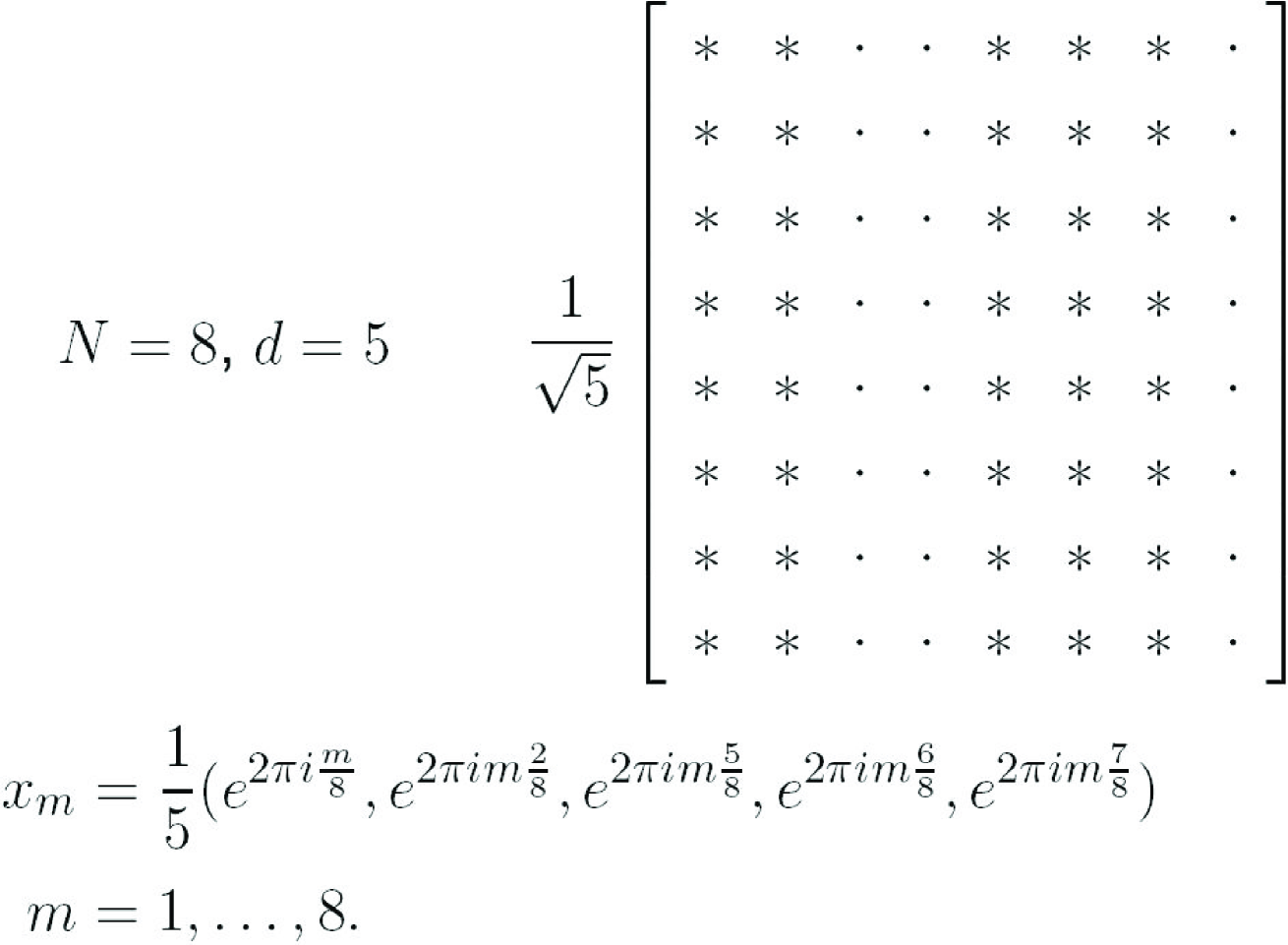
The rows of the $N\times d$ matrix in Definition 2.9, up to multiplication by ${1}/{\sqrt{d}},$ form a FUNTF for ${\mathbb{C}}^{d}.$ For example, see Figure 1, where $d=5$ and $N=8$. The function, $s$ of Definition 2.9 determines the 5 columns of $\ast$s, that, in turn, determine ${\mathbb{C}}^{5}$.

Figure 1. A DFT FUNTF

Also, for a given $N,$ we shall use the notation, $\omega=e_{-1}=e^{-2\pi i/N},$ and so $e_{m}=e^{2\pi im/N}$. Note that $\{e_{m}\}_{m=0}^{N-1}$ is a tight frame for ${\mathbb{C}}.$

3. The vector-valued discrete Fourier transform (DFT)

3.1. Definition and inversion theorem

In order to achieve the goals listed in Subsection 1.2, we shall also have to develop a vector-valued DFT theory to verify, not just motivate, that $A_{p}^{d}(u)$ is an STFT in the case $\{x_{k}\}_{k=0}^{N-1}$ is a DFT frame for ${\mathbb{C}}^{d}$.

We shall use the convention that the juxtaposition of vectors of equal dimension is the pointwise product of those vectors. Thus, for two functions, $u,v:{\mathbb{Z}}/N{\mathbb{Z}}\rightarrow\mathbb{C}^{d},$ we let $uv$ be the coordinate-wise product of $u$ and $v.$ This means that

$$\forall m\in{\mathbb{Z}}/N{\mathbb{Z}},\quad(uv)(m)=u(m)v(m)\in\mathbb{C}^{d},$$

where the product on the right is pointwise multiplication of vectors in $\ell^{2}({\mathbb{Z}}/d{\mathbb{Z}}),$ and so $u(m)(p),v(m)(p),(uv)(m)(p)\in{\mathbb{C}}$ for each $p\in{\mathbb{Z}}/d{\mathbb{Z}},$ i.e., $u(m)(p)$ designates the $p$th coordinate in $\mathbb{C}^{d}$ of the vector $u(m)\in\mathbb{C}^{d}.$

Definition 3.1 (Vector-valued discrete Fourier transform).

Let $\{x_{k}\}_{k=0}^{N-1}$ be a DFT frame for $\mathbb{C}^{d}$ with injective mapping $s.$ Given $u:\mathbb{{\mathbb{Z}}}/N{\mathbb{Z}}\rightarrow\mathbb{C}^{d},$ the vector-valued discrete Fourier transform (vector-valued DFT) $\widehat{u}$ of $u$ is defined by the formula,

(12) $$\forall n\in{\mathbb{Z}}/N{\mathbb{Z}},\quad F(u)(n)=\widehat{u}(n)=\sum_{m=0}^{N-1}u(m)x_{-mn}\in{\mathbb{C}}^{d},$$

where the product $u(m)x_{-mn}$ is pointwise (coordinate-wise) multiplication. Further, the mapping

$$F:\ell^{2}({\mathbb{Z}}/N{\mathbb{Z}}\times{\mathbb{Z}}/d{\mathbb{Z}})\rightarrow\ell^{2}({\mathbb{Z}}/N{\mathbb{Z}}\times{\mathbb{Z}}/d{\mathbb{Z}})$$

is a linear operator.

Remark 3.2.

a. Given $u:{\mathbb{Z}}/N{\mathbb{Z}}\rightarrow{\mathbb{C}}^{d}.$ We write $u\in\ell^{2}({\mathbb{Z}}/N{\mathbb{Z}}\times{\mathbb{Z}}/d{\mathbb{Z}})$ as a function of two arguments so that $u(m)(p)\in{\mathbb{C}}.$ With this notation we can think of $u$ and $\widehat{u}$ as $N\times d$ matrices with entries $u(m)(p)$ and $\widehat{u}(n)(q),$ respectively.

b. Thus, we have

$$\forall q\in{\mathbb{Z}}/d{\mathbb{Z}},\quad\widehat{u}(n)(q) =\left(\sum_{m=0}^{N-1}u(m)x_{-mn}\right)(q)$$

$$=\left(\sum_{m=0}^{N-1}u(m)(q)x_{-mn}(q)\right).$$

From this we see that $\widehat{u}(n)(q)$ depends only on $\{u(m)(q)\}_{m=0}^{N-1}$, i.e., when thought of as matrices the $q$-th column of $\widehat{u}$ depends only on the $q$-th column of $u$.

Theorem 3.3 (Inversion theorem).

The vector-valued DFT is invertible if and only if $s$, the injective function defining the DFT frame, has the property that

$$\forall n\in{\mathbb{Z}}/d{\mathbb{Z}},\quad(s(n),N)=1.$$

In this case, the inverse is given by

$$\forall\ m\in\mathbb{{\mathbb{Z}}}/N{\mathbb{Z}},\quad u(m)=(F^{-1}\widehat{u})(m)=\frac{1}{N}\sum_{p=0}^{N-1}\widehat{u}(p)x_{mp};$$

and we also have that $F^{\ast}F=FF^{\ast}=NI$, where $I$ is the identity operator.

Proof.

We first show the forward direction. Suppose there is $n_{0}\in{\mathbb{Z}}/d{\mathbb{Z}}$ such that $(s(n_{0}),N)\neq 1$. Then there exists $j,l,M\in{\mathbb{N}}$ such that $j>1$, $s(n_{0})=jl$, and $N=jM$. Define a matrix $A$ as

$$A=(e^{2\pi imks(n_{0})/N})_{m,k=0}^{N-1}=(e^{2\pi imkl/M})_{m,k=0}^{N-1}.$$

$A$ has rank strictly less than $N$ since the $0$-th and $M$-th rows are all $1$s. Therefore we can choose a vector $v\in{\mathbb{C}}^{N}$ orthogonal to the rows of $A$. Define $u:{\mathbb{Z}}/N{\mathbb{Z}}\rightarrow{\mathbb{C}}^{d}$ by

$$u(m)(n)=\begin{cases}v(m)&\text{ if }n=n_{0}\\ 0&\text{ otherwise.}\end{cases}$$

Then,

$$\forall n\neq n_{0},\quad\widehat{u}(m)(n) =\sum_{k=0}^{N-1}u(k)(n)x_{-mk}(n)=\sum_{k=0}^{N-1}0\cdot x_{-mk}(n)=0,$$

while, for $n=n_{0}$, we have

$$\widehat{u}(m)(n_{0})=\sum_{k=0}^{N-1}u(k)(n_{0})x_{-mk}(n_{0})=\sum_{k=0}^{N-1}u(k)(n_{0})e^{-2\pi imks(n_{0})/N}$$

$$=\sum_{k=0}^{N-1}u(k)(n_{0})e^{-2\pi imkl/M}=\langle{u(\cdot)(n_{0}),e^{2\pi im(\cdot)l/M}}\rangle=\langle{v,e^{2\pi im(\cdot)l/M}}\rangle=0.$$

The final equality follows from the fact that $v$ is orthogonal to the rows of $A$. Hence, the vector-valued DFT defined by $s$ has non-trivial kernel and is not invertible.

We prove the converse and the formula for the inverse with a direct calculation. We compute

$$\sum_{n=0}^{N-1}\widehat{u}(n)x_{mn} =\sum_{n=0}^{N-1}\left(\sum_{k=0}^{N-1}u(k)x_{-kn}\right)x_{mn}$$

$$=\sum_{k=0}^{N-1}\left(u(k)\left(\sum_{n=0}^{N-1}x_{n(m-k)}\right)\right).$$

The $r$-th component of the last summation is

$$\sum_{n=0}^{N-1}x_{n(m-k)}(r) =\sum_{n=0}^{N-1}e^{2\pi in(m-k)s(r)/N}$$

$$=\begin{cases}N&\text{if }(m-k)s(r)\equiv 0\text{ mod }N\\ 0&\text{if }(m-k)s(r)\not\equiv 0\text{ mod }N.\end{cases}$$

Since $(s(r),N)=1$, the first cases occurs if and only if $k=m$. Continuing with the previous calculation, we have

$$\sum_{k=0}^{N-1}\left(u(k)\left(\sum_{n=0}^{N-1}x_{n(m-k)}\right)\right)=Nu(m).$$

Finally, we compute the adjoint of $F$.

$$\langle{Fu,v}\rangle=\sum_{m=0}^{N-1}\sum_{n=0}^{d-1}\widehat{u}(m)(n)\overline{v(m)(n)}=\sum_{m=0}^{N-1}\sum_{n=0}^{d-1}\left(\sum_{k=0}^{N-1}u(k)(n)x_{-mk}(n)\right)\overline{v(m)(n)}$$

$$=\sum_{m=0}^{N-1}\sum_{n=0}^{d-1}\left(\sum_{k=0}^{N-1}u(k)(n)e^{-2\pi imks(n)/N}\right)\overline{v(m)(n)}=\sum_{k=0}^{N-1}\sum_{n=0}^{d-1}\left(\sum_{m=0}^{N-1}\overline{v(m)(n)e^{2\pi imks(n)/N}}\right)u(k)(n)$$

$$=\sum_{k=0}^{N-1}\sum_{n=0}^{d-1}u(k)(n)\overline{\left(\sum_{m=0}^{N-1}v(m)(n)x_{mk}(n)\right)}=\langle{u,F^{*}v}\rangle.$$

Therefore, $F^{*}$ is defined by

$$(F^{*}v)(k)=\sum_{m=0}^{N-1}v(m)x_{mk},$$

and $F^{*}=NF^{-1}$. ∎

By Theorem 3.3, we can define the unitary vector-valued discrete Fourier transform $\mathcal{F}$ by the formula

$$\mathcal{F}=\frac{1}{\sqrt{N}}F.$$

With this definition, we have

$$\mathcal{F}\mathcal{F}^{\ast}=\mathcal{F}^{\ast}\mathcal{F}=I,$$

and $\mathcal{F}$ is unitary .

Definition 3.4 (Translation and modulation).

Let $u:{\mathbb{Z}}/N{\mathbb{Z}}\rightarrow\mathbb{C}^{d}$, and let $\{x_{k}\}_{k=0}^{N-1}$ be a DFT frame for $\mathbb{C}^{d}$. For each $j\in{\mathbb{Z}}/N{\mathbb{Z}}$, define the translation operators,

$$\tau_{j}:\ell^{2}({\mathbb{Z}}/N{\mathbb{Z}}\times{\mathbb{Z}}/d{\mathbb{Z}})\rightarrow\ell^{2}({\mathbb{Z}}/N{\mathbb{Z}}\times{\mathbb{Z}}/d{\mathbb{Z}}),\quad\tau_{j}u(m)=u(m-j),$$

and the modulation operators,

$$e^{j}:{\mathbb{Z}}/N{\mathbb{Z}}\rightarrow\mathbb{C}^{d},\quad e^{j}(k)=x_{jk}.$$

The usual translation and modulation properties of the Fourier transform hold for the vector-valued transform.

Theorem 3.5.

Let $u:{\mathbb{Z}}/N{\mathbb{Z}}\rightarrow\mathbb{C}^{d}$, and let $\{x_{k}\}_{k=0}^{N-1}$ be a DFT frame for $\mathbb{C}^{d}$ with associated vector-valued discrete Fourier transform $F.$ Then,

$$F(\tau_{j}u)=e^{-j}\widehat{u}$$

and

$$F(e^{j}u)=\tau_{j}\widehat{u}.$$

Proof.

i. We compute

$$\widehat{\tau_{j}u}(n)=\sum_{m=0}^{N-1}\tau_{j}u(m)x_{-mn}=\sum_{m=0}^{N-1}u(m-j)x_{-mn}=\sum_{k=-j}^{N-1-j}u(k)x_{-(k+j)n}$$

$$=\sum_{k=0}^{N-1}u(k)x_{-kn-jn}=x_{-jn}\left(\sum_{k=0}^{N-1}u(k)x_{-kn}\right)=x_{-jn}\widehat{u}(n).$$

The third equality follows by setting $k=m-j$, the fourth by reordering the sum and noting that the index of summation is modulo $N$, and the fifth follows since $x_{j+k}=x_{j}x_{k}$ and by the bilinearity of pointwise products.

ii. We compute

$$\widehat{e^{j}u}(n)=\sum_{m=0}^{N-1}(e^{j}u)(m)x_{-mn}=\sum_{m=0}^{N-1}x_{jm}u(m)x_{-mn}$$

$$=\sum_{m=0}^{N-1}u(m)x_{-m(n-j)}\\ =\widehat{u}(n-j).$$

The third equality follows from commutativity and since $x_{j+k}=x_{j}x_{k}$. ∎

3.2. A matrix formulation of the vector-valued DFT

We now describe a different way of viewing the vector-valued DFT that makes some properties more apparent. Given $N\in{\mathbb{N}}$, define the matrices $\mathcal{D}_{\ell},$

$$\forall\ell\in{\mathbb{Z}}/N{\mathbb{Z}},\quad\mathcal{D}_{\ell}=(e^{-2\pi imn\ell/N})_{m,n=0}^{N-1}.$$

By definition of the vector-valued DFT, we have

$$\widehat{u}(n)(q)=\left(\sum_{m=0}^{N-1}u(m)(q)x_{-mn}(q)\right)$$

$$=\left(\sum_{m=0}^{N-1}u(m)(q)e^{-2\pi imns(q)/N}\right)=\left(\mathcal{D}_{s(q)}u(\cdot)(q)\right)(n),$$

i.e., the vector $\widehat{u}(\cdot)(q)$ is equal to the vector $\mathcal{D}_{s(q)}u(\cdot)(q)$. In other words, we obtain $\widehat{u}$ by applying the matrix $\mathcal{D}_{s(q)}$ to the $q$–th column of $u$ for each $0\leq q\leq d-1$. Therefore, $F$ is invertible if and only if each matrix $\mathcal{D}_{s(q)}$ is invertible.

The rows of $\mathcal{D}_{\ell}$ are a subset of the rows of the DFT matrix, and each row of the DFT matrix is a character of ${\mathbb{Z}}/N{\mathbb{Z}}$. Taken as a collection, the characters form the dual group $({\mathbb{Z}}/N{\mathbb{Z}}\widehat{)}\simeq{\mathbb{Z}}/N{\mathbb{Z}}$ under pointwise multiplication. With this group operation and the fact that

$$\forall m,n\in{\mathbb{Z}}/N{\mathbb{Z}},\quad e^{-2\pi imn\ell/N}=(e^{-2\pi in\ell/N})^{m},$$

we see the rows of $\mathcal{D}_{\ell}$ are the orbit of some element $\gamma\in({\mathbb{Z}}/N{\mathbb{Z}}\widehat{)}$ repeated $|\gamma|/N$ times. Hence, $\mathcal{D}_{\ell}$ is invertible if and only if $\gamma$ generates the entire dual group. From the theory of cyclic groups, $\gamma$ is a generator of $({\mathbb{Z}}/N{\mathbb{Z}}\widehat{)}$ if and only if $\gamma=(e^{-2\pi in\ell/N})_{n=0}^{N-1}$ for some $\ell$ relatively prime to $N$. Therefore, $F$ is invertible if and only if $s(q)$ is relatively prime to $N$ for each $q$.

Example 3.6.

Let $N=4$ and recall that $\omega=e^{-2\pi i/4}$. We compute the matrices $\mathcal{D}_{1},$ $\mathcal{D}_{2},$ and $\mathcal{D}_{3}.$

$$\mathcal{D}_{1}=\left(\begin{array}[]{cccc}1&1&1&1\\ 1&\omega&\omega^{2}&\omega^{3}\\ 1&\omega^{2}&1&\omega^{2}\\ 1&\omega^{3}&\omega^{2}&\omega\\ \end{array}\right)\quad\mathcal{D}_{2}=\left(\begin{array}[]{cccc}1&1&1&1\\ 1&\omega^{2}&1&\omega^{2}\\ 1&1&1&1\\ 1&\omega^{2}&1&\omega^{2}\\ \end{array}\right)\quad\mathcal{D}_{3}=\left(\begin{array}[]{cccc}1&1&1&1\\ 1&\omega^{3}&\omega^{2}&\omega\\ 1&\omega^{2}&1&\omega^{2}\\ 1&\omega^{1}&\omega^{2}&\omega^{3}\\ \end{array}\right)$$

It is easy to see that $\mathcal{D}_{1}$ and $\mathcal{D}_{3}$ are invertible while $\mathcal{D}_{2}$ is not invertible. In each case the matrix $\mathcal{D}_{i}$ is generated by pointwise powers of its second row, which have orders $4$, $2$, and $4$ respectively. In fact, the full vector-valued DFT can be viewed as a block matrix, where the $q$th block is $D_{s(q)}$.

3.3. The Banach algebra of the vector-valued DFT

We now study the vector-valued DFT in terms of Banach algebras. In fact, we shall define a Banach algebra structure on $\mathcal{A}=L^{1}({\mathbb{Z}}/N{\mathbb{Z}}\times{\mathbb{Z}}/d{\mathbb{Z}})$, describe the spectrum $\sigma(\mathcal{A})$ of $\mathcal{A},$ and then prove that the Gelfand transform of $\mathcal{A}$ is the vector-valued DFT.

To this end, first recall that if $G$ is a locally compact Abelian group (LCAG), then $L^{1}(G)$ is a commutative Banach algebra under convolution.

Next, let $\mathcal{B}$ be a commutative Banach $\ast$-algebra over ${\mathbb{C}},$ where $\ast$ indicates the involution satisfying the properties, $(x+y)^{\ast}=x^{\ast}+y^{\ast},(cx)^{\ast}=\overline{c}x^{\ast},(xy)^{\ast}=y^{\ast}x^{\ast},$ and $x^{\ast\ast}=x$ for all $x,y\in\mathcal{B}$ and $c\in{\mathbb{C}}.$ For example, let $\mathcal{B}=L^{1}(G)$ and define $f^{\ast}(t)=\overline{f(-t)}$ for $f\in L^{1}(G).$ The spectrum $\sigma(\mathcal{B})$ of $\mathcal{B}$ is the set of non-zero homomorphisms, $h:\mathcal{B}\rightarrow{\mathbb{C}}.$ $\sigma(\mathcal{B})$ is subset of the weak $\ast$-compact unit ball of the dual space ${\mathcal{B}}^{\prime}$ of the Banach space $\mathcal{B},$ and each $x\in\mathcal{B}$ defines a function $\widehat{x}:\sigma(\mathcal{B})\rightarrow{\mathbb{C}}$ given by

$$\forall h\in\sigma(\mathcal{B}),\quad\widehat{x}(h)=h(x).$$

$\widehat{x}$ is the Gelfand transform of $x.$ We shall use well-known properties of the Gelfand transform, e.g., see [69], [42], [73], [53], [54], [71], [38].

Using the group structure on ${\mathbb{Z}}/N{\mathbb{Z}}\times{\mathbb{Z}}/d{\mathbb{Z}},$ we define the convolution of $u,v\in\mathcal{A}=L^{1}({\mathbb{Z}}/N{\mathbb{Z}}\times{\mathbb{Z}}/d{\mathbb{Z}})$ by the formula,

(13) $$(u\ast v)(m)(n)=\sum_{k=0}^{N-1}\sum_{l=0}^{d-1}u(k)(l)v(m-k)(n-l).$$

This definition is not ideal for our purposes because it treats $u$ and $v$ as functions that take $Nd$ values. Our desire is to view $u$ and $v$ as functions that take $N$ values, that are each $d$ dimensional vectors. The convolution (13) can be rewritten as

$$(u\ast v)(m)(n)=\sum_{k=0}^{N-1}(u(k)\ast v(m-k))(n),$$

where the $\ast$ on the right hand side is $d$-dimensional convolution. Replacing this $d$-dimensional convolution with pointwise multiplication, we arrive at the following new definition of convolution on $\mathcal{A}.$

Definition 3.7 (Vector-valued convolution).

Let $u,v\in\mathcal{A}.$ Define the vector-valued convolution of $u$ and $v$ by the formula

$$(u\ast_{\rm v}v)(m)=\sum_{k=0}^{N-1}u(k)v(m-k).$$

Theorem 3.8.

$\mathcal{A}$ equipped with the vector-valued convolution $\ast_{\rm v}$ is a commutative Banach $\ast$-algebra with unit $e$ defined as

$$e(m)=\begin{cases}\vec{1}&m=0\\ \vec{0}&m\neq 0,\end{cases}$$

where $\vec{1}$ and $\vec{0}$ are the vectors of $1$s and $0$s, respectively, and with involution defined as $u^{\ast}(m)=\overline{u(-m)}.$

Proof.

It is essentially only necessary to verify that $\left\|u\ast_{\rm v}v\right\|_{1}\leq\left\|u\right\|_{1}\left\|v\right\|_{1}$ is valid. We compute

$$\left\|u\ast_{\rm v}v\right\|_{1}=\sum_{m=0}^{N-1}\left\|u\ast v(m)\right\|_{L^{1}({\mathbb{Z}}/d{\mathbb{Z}})}=\sum_{m=0}^{N-1}\left\|\sum_{k=0}^{N-1}u(k)v(m-k)\right\|_{L^{1}({\mathbb{Z}}/d{\mathbb{Z}})}$$

$$\leq\sum_{m=0}^{N-1}\sum_{k=0}^{N-1}\left\|u(k)v(m-k)\right\|_{L^{1}({\mathbb{Z}}/d{\mathbb{Z}})}\leq\sum_{m=0}^{N-1}\sum_{k=0}^{N-1}\left\|u(k)\right\|_{L^{1}({\mathbb{Z}}/d{\mathbb{Z}})}\left\|v(m-k)\right\|_{L^{1}({\mathbb{Z}}/d{\mathbb{Z}})}$$

$$=\sum_{k=0}^{N-1}\left\|u(k)\right\|_{L^{1}({\mathbb{Z}}/d{\mathbb{Z}})}\sum_{m=0}^{N-1}\left\|v(m-k)\right\|_{L^{1}({\mathbb{Z}}/d{\mathbb{Z}})}\\ =\sum_{k=0}^{N-1}\left\|u(k)\right\|_{L^{1}({\mathbb{Z}}/d{\mathbb{Z}})}\left\|v\right\|_{1}\\ =\left\|u\right\|_{1}\left\|v\right\|_{1}.$$

∎

Tying this together with our DFT theory, we have the following desired theorem relating $\mathcal{A}$ to the vector-valued DFT.

Theorem 3.9 (Convolution theorem).

Let $u,v\in\mathcal{A}$. The vector-valued Fourier transform of the convolution of $u$ and $v$ is the vector product of their Fourier transforms, i.e.,

$$F(u\ast_{\rm v}v)=F(u)F(v).$$

Proof.

$$F(u\ast_{\rm v}v)(n)=\sum_{m=0}^{N-1}(u\ast v)(m)x_{-mn}=\sum_{m=0}^{N-1}\left(\sum_{k=0}^{N-1}u(k)v(m-k)\right)x_{-mn}$$

$$=\sum_{k=0}^{N-1}u(k)\left(\sum_{m=0}^{N-1}v(m-k)x_{-mn}\right)=\sum_{k=0}^{N-1}u(k)\left(\sum_{l=0}^{N-1}v(l)x_{-(k+l)n}\right)$$

$$=\left(\sum_{k=0}^{N-1}u(k)x_{-kn}\right)\left(\sum_{l=0}^{N-1}v(l)x_{-ln}\right)\\ =F(u)(n)F(v)(n).$$

∎

We shall now describe the spectrum of $\mathcal{A}$ and the Gelfand transform of $\mathcal{A}$, see Theorem 3.10.

Define functions $\delta_{(i,j)}$ in $\mathcal{A}$ by

$$\delta_{(i,j)}(m)(n)=\begin{cases}1&(m,n)=(i,j)\\ 0&\text{otherwise}.\\ \end{cases}$$

It is easy to see that $\delta_{(1,j)}^{k}=\delta_{(1,j)}\ast\ldots\ast\delta_{(1,j)}\text{ (k factors) }=\delta_{(k,j)}$ so that $\{\delta_{(1,j)}\}_{j=0}^{d-1}$ generate $\mathcal{A}$. We shall find the spectrum of the individual elements of our generating set $\{\delta_{(1,j)}\}_{j=0}^{d-1}$, and with this information describe the spectrum of $\mathcal{A}$.

To find the spectrum of $\delta_{(1,j)}$ we first find necessary conditions on $\lambda$ for $(\lambda e-\delta_{(1,j)})^{-1}$ to exist, and when these conditions are met we compute $(\lambda e-\delta_{(1,j)})^{-1}$ and thereby show the conditions are sufficient as well. To that end, suppose $u=(\lambda e-\delta_{(1,j)})^{-1}$ exists, i.e., $(\lambda e-\delta_{(1,j)})\ast u=e$. Expanding the definitions on the left hand side

$$(\lambda e-\delta_{(1,j)})\ast u(m) =\sum_{k=0}^{N-1}(\lambda e-\delta_{(1,j)})(k)u(m-k)$$

$$=\lambda u(m)-\delta_{(1,j)}(1)u(m-1).$$

Setting the result equal to $e(m)$ and dividing into the cases $m=0$ and $m\neq 0$ yields two equations

(14) $$\forall n\in{\mathbb{Z}}/d{\mathbb{Z}},\quad\lambda u(0)(n)-\delta_{(1,j)}(1)(n)u(N-1)(n)=1$$

and

(15) $$\forall n\in{\mathbb{Z}}/d{\mathbb{Z}}\;{\rm and}\;\forall m\in{{\mathbb{Z}}/N{\mathbb{Z}}}\setminus\{0\},\quad\lambda u(m)(n)-\delta_{(1,j)}(1)(n)u(m-1)(n)=0.$$

Substituting $n=j$ into (14) yields

(16) $$\lambda u(0)(j)-u(N-1)(j)=1,$$

while for $n\neq j$ we have

$$u(0)(n)=\frac{1}{\lambda}.$$

Therefore, we must have $\lambda\neq 0$. Similarly, substituting $n=j$ in (15) gives

(17) $$\forall m\neq 0,\quad\lambda u(m)(j)-u(m-1)(j)=0,$$

while

$$\forall n\neq j,\;\forall m\neq 0,\quad u(m)(n)=0.$$

At this point and for our fixed $j$ we have specified all the values of $u$ except for $u(m)(j)$. Now, iterate (17) $N-1$ times to find

(18) $$\lambda^{N-1}u(N-1)(j)-u(0)(j)=0.$$

Finally, multiplying (18) by $\lambda$ and adding it to equation (16) we obtain

$$(\lambda^{N}-1)u(N-1)(j)=1,$$

and hence $\lambda^{N}\neq 1$. Using (17) we can find the remaining values of $u(m)(j)$:

$$u(m)(j)=\frac{\lambda^{N-m-1}}{\lambda^{N}-1}.$$

This completes the computation of $u$. We have shown that, for $\lambda e-\delta_{(1,j)}$ to be invertible, $\lambda$ must satisfy $\lambda\neq 0$ and $\lambda^{N}\neq 1$. Given that $\lambda$ meets these requirements we found an explicit inverse; therefore $\sigma(\delta_{(1,j)})=\{0,\lambda:\lambda^{N}=1\}.$

By the Riesz representation theorem, a linear functional on $\mathcal{A}$ is given by integration against a function $\gamma\in L^{\infty}({\mathbb{Z}}/N{\mathbb{Z}}\times{\mathbb{Z}}/d{\mathbb{Z}}),$ which we can also view simply as an $N\times d$ matrix. Further, a basic result in the Gelfand theory is that, for a commutative Banach algebra with unit, we have $\widehat{x}(\sigma(\mathcal{A}))=\sigma(x)$ (Theorem 1.13 of [38]). Combining this with our previous calculations, it follows that for a multiplicative linear functional $\gamma$,

$$\overline{\gamma(1)(n)}=\int\delta_{(1,n)}\overline{\gamma}=\gamma(\delta_{(1,n)})\in\sigma(\delta_{(1,n)}).$$

Since $\gamma$ is multiplicative,

$$\overline{\gamma(m)(n)}=\int\delta_{(m,n)}\overline{\gamma}=\int\delta_{(1,n)}^{m}\overline{\gamma}=\gamma(\delta_{(1,n)}^{m})=\gamma(\delta_{(1,n)})^{m},$$

taking the values $0$ or $\lambda^{m}$ where $\lambda^{N}=1.$ Therefore $\gamma(0)(n)$ is $0$ or $1$, and since

$$1=\gamma(e)=\sum_{k=0}^{d-1}\overline{\gamma(0)(k)},$$

we have $\gamma(0)(n)\neq 0$ (and thus $\gamma(1)(n)\neq 0$) for only one $n$. It follows that for this $n$, $\gamma(1)(n)=\overline{\lambda}$ where $\lambda^{N}=1$.

We have everything we need to describe $\sigma(\mathcal{A})$. The multiplicative linear functionals on $\mathcal{A}$ are $N\times d$ matrices of the form

$$\gamma_{\lambda,k}(m)(n)=\begin{cases}\lambda^{-m}&\text{for }n=k,\\ 0&\text{otherwise,}\end{cases}\quad\text{where }\lambda^{N}=1,\quad 0\leq k\leq d-1.$$

Set $\omega=e^{-2\pi i/N}$. If $\lambda^{N}=1$, then $\lambda=\omega^{j}$ for some $0\leq j\leq N-1$, and we can write $\gamma_{\lambda,k}$ as $\gamma_{j,k}$. Thus, we can list all the elements of $\sigma(\mathcal{A})$ as $\{\gamma_{j,k}\}$, $0\leq j\leq N-1$, $0\leq k\leq d-1$, and there are $Nd$ of them.

Let $s:{\mathbb{Z}}/d{\mathbb{Z}}\rightarrow{\mathbb{Z}}/N{\mathbb{Z}}$ be injective and have the property that for every $n\in{\mathbb{Z}}/d{\mathbb{Z}}$, $(s(n),N)=1$, i.e., the vector-valued DFT defined by $s$ is invertible. Using $s$, we can reorder $\sigma(\mathcal{A})$ as follows. For $0\leq p\leq N-1$ and $0\leq q\leq d-1,$ define $\gamma_{p,q}^{\prime}$ by

$$\gamma_{p,q}^{\prime}(m)(n)=\begin{cases}\omega^{-pms(q)}&\text{for }n=q,\\ 0&\text{otherwise}.\end{cases}$$

We claim $\{\gamma_{p,q}^{\prime}\}_{p,q}$ is a reordering of $\{\gamma_{j,k}\}_{j,k}$. To show this, first note that $\{\gamma_{p,q}^{\prime}\}_{p,q}\subseteq\{\gamma_{j,k}\}_{j,k}$. To demonstrate the reverse inclusion, for each $q\in{\mathbb{Z}}/d{\mathbb{Z}}$ find a multiplicative inverse to $s(q)$ in ${\mathbb{Z}}/N{\mathbb{Z}}$. This may be done because $(s(q),N)=1$ for every $q$. Writing this inverse as $s(q)^{-1},$ it follows that

$$\gamma_{js(k)^{-1},k}^{\prime}=\gamma_{j,k},$$

and therefore $\{\gamma_{j,k}\}_{j,k}\subseteq\{\gamma_{p,q}^{\prime}\}_{p,q}$.

We summarize all of these calculations as the following theorem.

Theorem 3.10 (Spectrum and Gelfand transform of $\mathcal{A}$).

The spectrum, $\sigma(\mathcal{A})$, of $\mathcal{A}$ is identified with ${\mathbb{Z}}/N{\mathbb{Z}}\times{\mathbb{Z}}/d{\mathbb{Z}}$ by means of the mapping $\gamma_{p,q}^{\prime}\leftrightarrow(p,q).$ Under this identification, the Gelfand transform, $\widehat{x}\in C(\sigma(\mathcal{A}))$, of $x\in\mathcal{A}$, is the $N\times d$ matrix,

$$\widehat{x}(p)(q)=\widehat{x}(\gamma_{p,q}^{\prime})=\gamma_{p,q}^{\prime}(x) =\sum_{m=0}^{N-1}x(m)(q)\omega^{pms(q)}$$

$$=\sum_{m=0}^{N-1}x(m)(q)e^{-2\pi ipms(q)/N}.$$

In particular, under the identification, $\gamma_{p,q}^{\prime}\leftrightarrow(p,q)$, the Gelfand transform of $\mathcal{A}$ is the vector-valued DFT.

While this shows that the transform we have defined is itself not new, it also shows that a classical transform can be redefined in the context of frame theory.

4. Formulation of generalized scalar- and vector-valued ambiguity functions

4.1. Formulation

Given $u:{\mathbb{Z}}/N{\mathbb{Z}}\rightarrow{\mathbb{C}}^{d}.$ A periodic vector-valued ambiguity function $A_{p}^{d}(u):{\mathbb{Z}}/N{\mathbb{Z}}\times{\mathbb{Z}}/N{\mathbb{Z}}\rightarrow{\mathbb{C}}^{d}$ was defined in [10] by observing the following. If $d=1$, then $A_{p}(u)$ in Equation (2) can be written as

$$A_{p}(u)(m,n) =\frac{1}{N}\sum_{k=0}^{N-1}\langle u(m+k),u(k)e_{kn}\rangle$$

(19) $$=\frac{1}{N}\sum_{k=0}^{N-1}\langle\tau_{-m}u(k),F^{-1}(\tau_{n}\widehat{u})(k)\rangle,$$

where $\tau_{-m}$ is the translation operator of Definition 3.4 and where $F^{-1}$ is the inverse DFT on ${\mathbb{Z}}/N{\mathbb{Z}}$. In particular, we see that $A_{p}(u)$ has the form of a STFT, see Example 4.3. This is central to our approach.

If $d>1$, then, motivated by the calculation $(\ref{eq:discreteambiguityrewrite}),$ it turns out that we can define both a ${\mathbb{C}}$-valued ambiguity function $A_{p}^{1}(u)$ and a ${\mathbb{C}}^{d}$-valued function $A_{p}^{d}(u).$

First, we consider the case of a ${\mathbb{C}}$-valued ambiguity function. Inspired by (4.1), and for $u:{\mathbb{Z}}/N{\mathbb{Z}}\rightarrow{\mathbb{C}}^{d}$, we wish to construct a sequence $\{x_{n}\}_{n=0}^{N-1}\subseteq{\mathbb{C}}^{d}$ and define a vector multiplication $\ast$ in ${\mathbb{C}}^{d}$ so that the mapping, $A_{p}^{1}(u):{\mathbb{Z}}/N{\mathbb{Z}}\times{\mathbb{Z}}/N{\mathbb{Z}}\rightarrow{\mathbb{C}},$ given by

(20) $$A_{p}^{1}(u)(m,n)=\frac{1}{N}\sum_{k=0}^{N-1}\langle u(m+k),u(k)\ast x_{kn}\rangle$$

is a meaningful ambiguity function. The product, $kn,$ is modular multiplication in ${\mathbb{Z}}/N{\mathbb{Z}}.$ In Subsections 4.2 and 4.4, we shall see that in quite general circumstances, for the proper $\{x_{n}\}_{n=0}^{N-1}$ and $\ast,$ Equation (20) can be made compatible with that of $A_{p}(u)$ in (4.1).

Second, we consider the case of a ${\mathbb{C}}^{d}$-valued ambiguity function. In the context of our definition of $A_{p}^{1}(u),$ we formulate the vector-valued version, $A_{p}^{d}(u),$ of the periodic ambiguity function as follows. Let $u:{\mathbb{Z}}/N{\mathbb{Z}}\rightarrow{\mathbb{C}}^{d}$, and define the mapping, $A_{p}^{d}(u):{\mathbb{Z}}/N{\mathbb{Z}}\times{\mathbb{Z}}/N{\mathbb{Z}}\rightarrow{\mathbb{C}}^{d},$ by

(21) $$A_{p}^{d}(u)(m,n)=\frac{1}{N}\sum_{k=0}^{N-1}u(m+k)\ast\overline{u(k)}\ast\overline{x_{kn}},$$

where $\{x_{n}\}_{n=0}^{N-1}$ and $\ast$ must also be constructed and defined, respectively. In Example 4.3, we shall see that this definition is compatible with that of $A_{p}(u)$ in (4.1).

To this end of defining $A_{p}^{d}(u),$ and motivated by the facts that $\{e_{n}\}_{n=0}^{N-1}$ is a tight frame for ${\mathbb{C}}$ (as noted in Subsection 2.4) and $e_{m}e_{n}=e_{m+n}$, the following frame multiplication assumptions were made in [10].

• There is a sequence $X=\{x_{n}\}_{n=0}^{N-1}\subseteq{\mathbb{C}}^{d}$ and a multiplication $\ast:{\mathbb{C}}^{d}\times{\mathbb{C}}^{d}\rightarrow{\mathbb{C}}^{d}$ such that

  (22) $$\forall m,n\in{\mathbb{Z}}/N{\mathbb{Z}},\quad x_{m}\ast x_{n}=x_{m+n};$$

• $X=\{x_{n}\}_{n=0}^{N-1}$ is a tight frame for ${\mathbb{C}}^{d};$

• The multiplication $\ast$ is bilinear, in particular,

  $$\left(\sum_{j=0}^{N-1}c_{j}x_{j}\right)\ast\left(\sum_{k=0}^{N-1}d_{k}x_{k}\right)=\sum_{j=0}^{N-1}\sum_{k=0}^{N-1}c_{j}d_{k}x_{j}\ast x_{k}.$$

There exist tight frames satisfying these assumptions, e.g., DFT frames. We shall characterize such tight frames and multiplications in Sections 5, 6, and 7.

A reason we developed our vector-valued DFT theory of Section 3 was to verify, not just motivate, that $A_{p}^{d}(u)$ is a STFT in the case $\{x_{k}\}_{k=0}^{N-1}$ is a DFT frame for ${\mathbb{C}}^{d}$. Let $X=\{x_{n}\}_{n=0}^{N-1}$ be a DFT frame for ${\mathbb{C}}^{d}$. We can leverage the relationship between the bilinear product pointwise multiplication and the operation of addition on the indices of $X$, i.e., $x_{m}x_{n}=x_{m+n}$, to define the periodic vector-valued ambiguity function $A_{p}^{d}(u)$ as in Equation (21). In this case, the DFT frame is acting as a high dimensional analog to the roots of unity $\{\omega_{n}=e^{2\pi in/N}\}_{n=0}^{N-1}$, that appear in the definition of the usual periodic ambiguity function.

Example 4.1 (Multiplication problem).

Given $u:{\mathbb{Z}}_{N}\longrightarrow{\mathbb{C}}^{d}$. If $d=1$ and $x_{n}=e^{2\pi in/N}$, then Equations (2) and (4.1) can be written as

$$A_{p}(u)(m,n)=\frac{1}{N}\sum_{k=0}^{N-1}\langle u(m+k),u(k)x_{nk}\rangle.$$

The multiplication problem for $A_{p}^{1}(u)$ is to characterize sequences $\{x_{k}\}\subseteq{\mathbb{C}}^{d}$ and multiplications $\ast$ so that

$$A_{p}^{1}(u)(m,n)=\frac{1}{N}\sum_{k=0}^{N-1}\langle u(m+k),u(k)\ast x_{nk}\rangle\in{\mathbb{C}}$$

is a meaningful and well-defined ambiguity function. This formula is clearly motivated by the STFT. It is for this reason that we made the frame multiplication assumptions.

In fact, suppose $\{x_{j}\}_{j=0}^{N-1}\subseteq{\mathbb{C}}^{d}$ satisfies the three frame multiplication assumptions. If we are given $u,v:{\mathbb{Z}}/N{\mathbb{Z}}\longrightarrow{\mathbb{C}}^{d}$ and $m,n\in{\mathbb{Z}}/N{\mathbb{Z}},$ then we can make the calculation,

$$u(m)*v(n) = \frac{d}{N}\sum_{j=0}^{N-1}\langle u(m),x_{j}\rangle x_{j}*\frac{d}{N}\sum_{s=0}^{N-1}<v(n),x_{s}>x_{s}$$

$$= \frac{d^{2}}{N^{2}}\sum_{j=0}^{N-1}\sum_{s=0}^{N-1}<u(m),x_{j}><v(n),x_{s}>x_{j}*x_{s}$$

$$= \frac{d^{2}}{N^{2}}\sum_{j=0}^{N-1}\sum_{s=0}^{N-1}\langle u(m),x_{j}\rangle\langle v(n),x_{s}\rangle x_{j+s}.$$

This allows us to formulate $A_{p}^{1}(u),$ as written in Equation (20), see Subsection 4.2.

4.2. $A_{1}^{d}(u)$ and $A_{p}^{d}(u)$ for DFT frames

Example 4.2 (STFT formulation of $A_{p}^{1}(u)$).

Given $u,v:{\mathbb{Z}}/N{\mathbb{Z}}\rightarrow\mathbb{C}^{d}$, and let $X=\{x_{k}\}_{k=0}^{N-1}\subseteq{\mathbb{C}}^{d}$ be a DFT frame for $\mathbb{C}^{d}$. Suppose $\ast$ denotes pointwise (coordinatewise) multiplication times a factor of $\sqrt{d}$. Then, the frame multiplication assumptions are satisfied. To see this, and without loss of generality, choose the first $d$ columns of the $N\times N$ DFT matrix, and let $r$ designate a fixed column. Then, we can verify the first of the frame multiplication assumptions by the following calculation, where the first step is a consequence of Equation (4.1):

$$x_{m}\ast x_{n}(r)=\frac{d^{2}}{N^{2}}\sum_{j=0}^{N-1}\sum_{s=0}^{N-1}\langle x_{m},x_{j}\rangle\langle x_{n},x_{s}\rangle x_{j+s}(r).$$

$$=\frac{1}{N^{2}\sqrt{d}}\sum_{j=0}^{N-1}\sum_{s=0}^{N-1}\sum_{t=0}^{d-1}\sum_{k=0}^{d-1}x_{(m-j)t}x_{(n-s)k}x_{(j+s)r}$$

$$=\frac{1}{N^{2}\sqrt{d}}\sum_{t=0}^{d-1}\sum_{k=0}^{d-1}x_{mt+nk}\sum_{j=0}^{N-1}x_{(r-t)j}\sum_{s=0}^{N-1}x_{(r-k)s}$$

$$=\frac{1}{N^{2}\sqrt{d}}\sum_{t=0}^{d-1}\sum_{k=0}^{d-1}x_{mt+nk}N\delta(r-t)N\delta(r-k)$$

$$=\frac{x_{(m+n)r}}{\sqrt{d}}=x_{m+n}(r).$$

The second and third frame multiplication assumptions follow since $X$ is a DFT frame and by a straightforward calculation (already used in Equation (4.1)), respectively.

Thus, in this case, $A_{p}^{1}(u)$ is well-defined for $u:\mathbb{{\mathbb{Z}}}/N{\mathbb{Z}}\rightarrow\mathbb{C}^{d}$ by Equation (24) since its right side exists:

(24) $$A_{p}^{1}(u)(m,n)=\frac{1}{N}\sum_{k=0}^{N-1}\langle u(m+k),u(k)\ast x_{nk}\rangle$$

$$=\frac{1}{N}\sum_{k=0}^{N-1}\left<u(m+k),\frac{d}{N}\sum_{j=0}^{N-1}<u(k),x_{j}>x_{j}*x_{nk}\right>$$

$$=\frac{d}{N^{2}}\sum_{k=0}^{N-1}\sum_{j=0}^{N-1}\langle x_{j},u(k)\rangle\langle u(m+k),x_{j+nk}\rangle.$$

Example 4.3 (STFT formulation of $A_{p}^{d}(u)$).

Given $u,v:{\mathbb{Z}}/N{\mathbb{Z}}\rightarrow\mathbb{C}^{d}$, and let $X=\{x_{k}\}_{k=0}^{N-1}\subseteq{\mathbb{C}}^{d}$ be a DFT frame for $\mathbb{C}^{d}$. Suppose $\ast$ denotes pointwise (coordinatewise) multiplication with a factor of $\sqrt{d}$. Then, the frame multiplication assumptions are satisfied. Utilizing the modulation functions, $e^{j},$ defined in Definition 3.4, we compute the right side of Equation (21) to obtain

(25) $$A_{p}^{d}(u)(m,n)=\frac{1}{N}\sum_{k=0}^{N-1}\tau_{-m}u(k)\overline{u(k)e^{n}(k)}.$$

Furthermore, the modulation and translation properties of the vector-valued DFT allow us to write Equation (25) as

$$A_{p}^{d}(u)(m,n)=\frac{1}{N}\sum_{k=0}^{N-1}(\tau_{m}u(k))\ast\overline{F^{-1}(\tau_{n}\hat{u})(k)};$$

and, notationally, we write the right side as the generalized inner product,

$$\frac{1}{N}\sum_{k=0}^{N-1}\{\tau_{m}u(k),F^{-1}(\tau_{n}\hat{u})(k)\},$$

where $\{u,v\}=u\overline{v}$ is coordinatewise multiplication for $u,v\in{\mathbb{C}}^{d}.$ Because of the form of Equation (21), we reiterate that $A_{p}^{d}(u)$ is compatible with the point of view of defining a vector-valued ambiguity function in the context of the STFT.

4.3. A generalization of the frame multiplication assumptions

In the previous DFT examples, $\ast$ is intrinsically related to modular addition defined on the indices of the frame elements, viz., $x_{m}\ast x_{n}=x_{m+n}$. Suppose we are given $X$ and $\ast,$ that satisfy the frame multiplication assumptions. It is not pre-ordained that the operation on the indices of the frame $X$, induced by the bilinear vector multiplication, be addition mod $N$, as is the case for DFT frames. We are interested in finding tight frames whose behavior is similar to that of DFT frames and whose index sets are Abelian groups, non-Abelian groups, or more general non-group sets and operations.

Hence, and being formulaic, we could have ${x}_{m}\ast{{x}_{n}}={x}_{m\bullet n}$ for some function $\bullet:{\mathbb{Z}}/N{\mathbb{Z}}\times{\mathbb{Z}}/N{\mathbb{Z}}\rightarrow{\mathbb{Z}}/N{\mathbb{Z}},$ and, thereby, we could use non-DFT frames or even non-FUNTFs for ${\mathbb{C}}^{d}$. Further, $\bullet$ could be defined on index sets, that are more general than ${\mathbb{Z}}/N{\mathbb{Z}}.$ Thus, a particular case could have the setting of bilinear mappings of frames for Hilbert spaces that are indexed by groups.

For the purpose of Subsection 4.4, we continue to consider the setting of ${\mathbb{Z}}/N{\mathbb{Z}}$ and ${\mathbb{C}}^{d}$, but replace the first frame multiplication assumption, Equation (22), by the formula,

(26) $$\forall m,n\in{\mathbb{Z}}/N{\mathbb{Z}},\quad x_{m}\ast x_{n}=x_{m\bullet n},$$

where $X=\{x_{k}\}_{k=0}^{N-1}$ is still a tight frame for ${\mathbb{C}}^{d}$ and where $\ast$ continues to be bilinear.

The formula, Equation (26), not only hints at generalization by the cross-product example of Subsection 4.4, but is the formal basis of the theory of frame multiplication in Sections 5, 6, and 7.

4.4. Frame multiplication assumptions for cross product frames

Let $\ast:\mathbb{C}^{3}\times\mathbb{C}^{3}\rightarrow{\mathbb{C}}^{3}$ be the cross product on $\mathbb{C}^{3}$ and let $\{i,j,k\}$ be the standard basis, e.g., $i=(1,0,0)\in{\mathbb{C}}^{3}.$ Therefore, we have

(27) $$i\ast j=k,j\ast i=-k,k\ast i=j,i\ast k=-j,j\ast k=i,k\ast j=-i,$$

$$i\ast i=j\ast j=k\ast k=0.$$

The union of two tight frames and the zero vector is a tight frame, so if we let $X=\{x_{n}\}_{n=0}^{6},$ where $x_{0}=0,x_{1}=i,x_{2}=j,x_{3}=k,x_{4}=-i,x_{5}=-j,x_{6}=-k,$ then it is straightforward to check that $X$ is a tight frame for ${\mathbb{C}}^{3}$ with frame bound $2.$

The index operation corresponding to the frame multiplication is

(28) $$\bullet:{\mathbb{Z}}/7{\mathbb{Z}}\times{\mathbb{Z}}/7{\mathbb{Z}}\longrightarrow{\mathbb{Z}}/7{\mathbb{Z}},$$

where $\bullet$ is the non-Abelian, non-group operation defined by the following table:

$1\bullet 2=3$,	$1\bullet 3=5$	$1\bullet 4=0$,	$1\bullet 5=6$,	$1\bullet 6=2$,
$2\bullet 1=6$,	$2\bullet 3=1$,	$2\bullet 4=3$,	$2\bullet 5=0$,	$2\bullet 6=4$,
$3\bullet 1=2$,	$3\bullet 2=4$,	$3\bullet 4=5$,	$3\bullet 5=1$,	$3\bullet 6=0$,
$n\bullet n=0$,		$n\bullet 0=0\bullet n=0$.

We have chosen this definition of $\bullet$ for the following reasons. As we saw in Example 4.1, the three frame multiplication assumptions are essential for defining a meaningful ambiguity function. In Subsection 4.1, these assumptions were based on the formula, $x_{m}\ast x_{n}=x_{m+n},$ used in Equation (22). However, in order to generalize this point of view, we shall consider the formula, $x_{m}\ast x_{n}=x_{m\bullet n},$ as indicated in Subsection 4.3. provided the corresponding three frame multiplication assumptions can be verified. In fact, for this cross product example, it is easily checked that the frame multiplication assumptions of Equation (22) are valid when $+$ is replaced by the $\bullet$ operation defined above in (28) and the corresponding table.

Consequently,we can write the cross product as

(29) $$\forall u,v\in{\mathbb{C}}^{3},\quad u\times v=u\ast v=\frac{1}{2^{2}}\sum_{s=1}^{6}\sum_{t=1}^{6}\langle u,x_{s}\rangle\langle v,x_{t}\rangle x_{s\bullet t}.$$

$$=\frac{1}{4}\sum_{n=1}^{6}\left(\sum_{j\bullet k=n}\langle{u,x_{j}}\rangle\langle{v,x_{k}}\rangle\right)x_{n}.$$

One possible application of the above is that, given frame representations for $u,v\in{\mathbb{C}}^{3},$ Equation (29) allows us to compute the frame representation of $u\times v$ without the process of going back and forth between the frame representations and their standard orthogonal representations.

There are five non-isomorphic groups of order 8: the Abelians (${\mathbb{Z}}/8{\mathbb{Z}},{\mathbb{Z}}/4{\mathbb{Z}}\times{\mathbb{Z}}/2{\mathbb{Z}},{\mathbb{Z}}/2{\mathbb{Z}}\times{\mathbb{Z}}/2{\mathbb{Z}}\times{\mathbb{Z}}/2{\mathbb{Z}}$), the dihedral, cf. Example 6.10, and the quaternion group $Q=\{\pm 1,\pm i,\pm j,\pm k\}.$ The unit of $Q$ is $1,$ the products $ij,$ etc. are the cross product as in Equation (27), and $ii=jj=kk=1.$ Clearly, $Q$ is closely related to $X=\{x_{n}\}_{n=0}^{6},$

5. Frame multiplication

We now define the notion of a frame multiplication, that is connected with a bilinear product on the frame elements, and we analyze its properties.

Definition 5.1 (Frame multiplication).

Let $X=\{x_{j}\}_{j\in J}$ be a frame for a $d-$dimensional Hilbert space $H$ over ${\mathbb{F}}$, and let $\bullet:J\times J\rightarrow J$ be a binary operation. The mapping $\bullet$ is a frame multiplication for $X$ or, by abuse of language, a frame multiplication for $H$, if it extends to a bilinear product $\ast$ on all of $H$, i.e., if there exists a bilinear product $\ast:H\times H\rightarrow H$ such that

$$\forall j,k\in J,\quad x_{j}\ast x_{k}=x_{j\bullet k}.$$

If $(G,\bullet)$ is a group, where $G=J$ and $\bullet$ is a frame multiplication for $X$, then we shall also say that $G$ defines a frame multiplication for $X.$

To fix ideas, we shall only deal with frame multiplication for finite dimensional Hilbert spaces, but our theory clearly extends, and many of the results are valid for infinite dimensional Hilbert spaces.

Let $X=\{x_{j}\}_{j\in J}$ be a frame for a $d-$dimensional Hilbert space $H.$ By definition, a binary operation $\bullet:J\times J\rightarrow J$ is a frame multiplication for $X$ when it extends to a bilinear product by bilinearity to the entire space $H$. Conversely, if there is a bilinear product $\ast:H\times H\rightarrow H$ which agrees with $\bullet$ on $X,$ i.e., $x_{j}\ast x_{k}=x_{j\bullet k}$, then it must be the unique extension given by bilinearity since $X$ spans $H$. Therefore, $\bullet$ defines a frame multiplication for $X$ if and only if for every $x=\sum_{i}a_{i}x_{i}\in H$ and $y=\sum_{i}b_{i}x_{i}\in H$,

(30) $$x\ast y=\sum_{i\in J}\sum_{j\in J}a_{i}b_{j}x_{i\bullet j}$$

is defined and independent of the frame representations used for $x$ and $y$.

Remark 5.2.

Whether or not a particular binary operation is a frame multiplication depends not just on the elements of the frame but on the indexing of the frame. For clarity of definitions and later theorems, we make no attempt to define a notion of frame multiplication for multi-sets of vectors that is independent of the index set.

A distinction that must be kept in mind is that $\bullet$ is a set operation on the indices of a frame while $\ast$ is a bilinear vector product defined on all of $H$.

We shall investigate the interplay between bilinear vector products on $H$, frames for $H$ indexed by $J$, and binary operations on $J$. For example, if we fix a binary operation $\bullet$ on $J$, then for what sort of frames indexed by $J$ do we obtain a frame multiplication? Conversely, if we fix a frame $X=\{x_{j}\}_{j\in J}$ for $H,$ then what sort of binary operations on $J$ are frame multiplications for $H$?

Proposition 5.3.

Let $X=\{x_{j}\}_{j\in J}$ be a frame for a $d$-dimensional Hilbert space $H,$ and let $\bullet:J\times J\rightarrow J$ be a binary operation. Then, $\bullet$ is a frame multiplication for $X$ if and only if

(31) $$\forall\{a_{i}\}_{i\in J}\subseteq{\mathbb{F}}\;{\rm and}\;\forall j\in J,\quad\sum_{i\in J}a_{i}x_{i}=0\,{\rm implies}\,\sum_{i\in J}a_{i}x_{i\bullet j}=0\,{\rm and}\,\sum_{i\in J}a_{i}x_{j\bullet i}=0.$$

Proof.

Suppose $\ast$ is the bilinear product defined by $\bullet$ and $\{a_{i}\}_{i\in J}$ is a sequence of scalars. If $\sum_{i\in J}a_{i}x_{i}=0$, then

$$\sum_{i\in J}a_{i}x_{i\bullet j}=\sum_{i\in J}a_{i}\left(x_{i}\ast x_{j}\right)=\left(\sum_{i\in J}a_{i}x_{i}\right)\ast x_{j}=0\ast x_{j}=0.$$

Similarly, by multiplying on the left by $x_{j}$, we see that $\sum_{i\in J}a_{i}x_{j\bullet i}=0.$

For the converse, suppose that statement (31) holds and $x=\sum_{i}a_{i}x_{i}=\sum_{i}c_{i}x_{i}$, $y=\sum_{j}b_{j}x_{j}=\sum_{j}d_{j}x_{j}$ $\in H$. By (31), we have

(32) $$\forall j\in J,\quad\sum_{i\in J}(a_{i}-c_{i})x_{i\bullet j}=0$$

and

(33) $$\forall i\in J,\quad\sum_{j\in J}(b_{j}-d_{j})x_{i\bullet j}=0.$$

Therefore, using (33) and (32), we obtain

$$\sum_{i\in J}\sum_{j\in J}a_{i}b_{j}x_{i\bullet j}=\sum_{i\in J}a_{i}\sum_{j\in J}b_{j}x_{i\bullet j}=\sum_{i\in J}a_{i}\sum_{j\in J}d_{j}x_{i\bullet j}$$

$$=\sum_{j\in J}d_{j}\sum_{i\in J}a_{i}x_{i\bullet j}=\sum_{j\in J}d_{j}\sum_{i\in J}c_{i}x_{i\bullet j}=\sum_{i\in J}\sum_{j\in J}c_{i}d_{j}x_{i\bullet j},$$

and, hence, $\ast$ is well-defined by (30). ∎

Definition 5.4 (Similarity).

Frames $X=\{x_{j}\}_{j\in J}$ and $Y=\{y_{j}\}_{j\in J}$ for a $d$-dimensional Hilbert space $H$ are similar if there exists an invertible linear operator $A\in\mathcal{L}(H)$ (see Appendix 9) such that

$$\forall j\in J,\quad Ax_{j}=y_{j}.$$

Proposition 5.5.

Suppose $X=\{x_{j}\}_{j\in J}$ and $Y=\{y_{j}\}_{j\in J}$ are frames for a $d$-dimensional Hilbert space $H,$ and that $X$ is similar to $Y$. Then, a binary operation $\bullet:J\times J\rightarrow J$ is a frame multiplication for $X$ if and only if it is a frame multiplication for $Y$.

Proof.

Because $A^{-1}y_{j}=x_{j}$ and $A^{-1}$ is also an invertible operator, we need only prove one direction of the proposition. Suppose $\bullet$ is a frame multiplication for $X$ and that $\sum_{i}a_{i}y_{i}=0$. We have

$$0=\sum_{i\in J}a_{i}y_{i}=\sum_{i\in J}a_{i}Ax_{i}=A\left(\sum_{i\in J}a_{i}x_{i}\right),$$

and since $A$ is invertible it follows that $\sum_{i}a_{i}x_{i}=0$. By Proposition 5.3, and because $\bullet$ is a frame multiplication for $X$, we can assert that

$$\forall j\in J,\quad\sum_{i\in J}a_{i}x_{i\bullet j}=0\text{ and }\sum_{i\in J}a_{i}x_{j\bullet i}=0.$$

Applying $A$ to both of these equations yields:

$$\forall j\in J,\quad\sum_{i\in J}a_{i}y_{i\bullet j}=0\text{ and }\sum_{i\in J}a_{i}y_{j\bullet i}=0.$$

Therefore, by Proposition 5.3, $\bullet$ is a frame multiplication for $Y$. ∎

Definition 5.6 (Multiplications of a frame).

Let $X=\{x_{j}\}_{j\in J}$ be a frame for a $d$-dimensional Hilbert space $H$. The multiplications of $X$ are defined and denoted by

$${\rm mult}(X)=\{{\rm frame}\,{\rm multiplications}\;\bullet:J\times J\rightarrow J\;{\rm for}\,X\}.$$

${\rm mult}(X)$ can be all functions (for example when $X$ is a basis), empty, or somewhere in-between.

Example 5.7.

Let $\alpha,\beta>0$, $\alpha\neq\beta$, and $\alpha+\beta<1$. Define $X_{\alpha,\beta}=\{x_{1}=(1,0)^{t},x_{2}=(0,1)^{t},x_{3}=\left(\alpha,\beta\right)^{t}\}$. Notationally, the superscript $t$ denotes the transpose of a vector. Then, $X_{\alpha,\beta}$ is a frame for ${\mathbb{C}}^{2}$ and ${\rm mult}(X_{\alpha,\beta})=\emptyset$. A straightforward way to prove that ${\rm mult}(X_{\alpha,\beta})=\emptyset$ is to show that there are no bilinear operations on ${\mathbb{C}}^{2}$ which leave $X_{\alpha,\beta}$ invariant. Suppose $\ast$ were such a bilinear operation. We shall obtain a contradiction.

First, we have the linear relation $x_{3}=\alpha x_{1}+\beta x_{2}$. Hence, by the bilinearity of $\ast$,

(34) $$x_{1}\ast x_{3}=\alpha x_{1}\ast x_{1}+\beta x_{1}\ast x_{2}.$$

Second, $\left\|x_{1}\right\|_{2}=\left\|x_{2}\right\|_{2}=1$ and $\left\|x_{3}\right\|_{2}<1$, where the inequality follows from the facts that $\left\|x_{3}\right\|_{2}=(\alpha^{2}+\beta^{2})^{1/2}$ and

$$0<\alpha^{2}+\beta^{2}=(\alpha+\beta)^{2}-2\alpha\beta<(\alpha+\beta)^{2}<1.$$

By the properties of $\alpha,\,\beta$, and using Equation (34), we have that

(35) $$\exists\,m,\,n\;{\rm such}\,{\rm that}\;\left\|x_{1}\ast x_{3}\right\|_{2}=\left\|\alpha x_{1}\ast x_{1}+\beta x_{1}\ast x_{2}\right\|_{2}$$

$$=\left\|\alpha x_{m}+\beta x_{n}\right\|_{2}\leq\alpha\left\|x_{m}\right\|_{2}+\beta\left\|x_{n}\right\|_{2}<1.$$

Thus, since $\ast$ leaves $X_{\alpha,\beta}$ invariant, we obtain that $x_{1}\ast x_{3}=x_{3}$ by (35). Furthermore, substituting $x_{3}$ for $x_{1}\ast x_{3}$ in Equation (34) and using the assumption that $\alpha\neq\beta$, yield $x_{1}\ast x_{1}=x_{1}$ and $x_{1}\ast x_{2}=x_{2}$. Performing the analogous calculation on $x_{3}\ast x_{2},$ in place of $x_{1}\ast x_{3}$ above, shows that $x_{2}\ast x_{2}=x_{2}$ and $x_{1}\ast x_{2}=x_{1},$ the desired contradiction.

Figure 2. The frame $X_{\alpha,\beta}$ from Example 5.7 for $\alpha=1/2$ and $\beta=1/4$. This frame has no frame multiplications.

Of particular interest, Proposition 5.5 tells us that the canonical dual frame $\{S^{-1}x_{j}\}_{j\in J}$ and the canonical tight frame $\{S^{-1/2}x_{j}\}_{j\in J}$ share the same frame multiplications as the original frame $X$. Because of this, we shall focus our attention on tight frames. An invertible element $V\in\mathcal{L}(H)$ mapping an $A$-tight frame $X=\{x_{j}\}$ (frame constant $A$) to an $A^{\prime}$-tight frame $Y=\{y_{j}\}$, as in Proposition 5.5, is a positive multiple of some $U\in\mathcal{U}(H),$ the space of unitary operators on $H,$ see Appendix 9. Indeed, we have

$$A\left\|V^{\ast}x\right\|^{2}=\sum_{j\in J}\left|\langle{V^{\ast}x,x_{j}}\rangle\right|^{2}=\sum_{j\in J}\left|\langle{x,Vx_{j}}\rangle\right|^{2}=\sum_{j\in J}\left|\langle{x,y_{j}}\rangle\right|^{2}=A^{\prime}\left\|x\right\|^{2}.$$

This leads us to a notion of equivalence for tight frames that sounds stronger than similarity but is actually just the restriction of similarity to the class of tight frames.

Definition 5.8 (Equivalence of tight frames).

Tight frames $X=\{x_{j}\}_{j\in J}$ and $Y=\{y_{j}\}_{j\in J}$ for a separable Hilbert space $H$ are unitarily equivalent if there is $U\in\mathcal{U}(H)$ and a positive constant $c$ such that

$$\forall j\in J,\quad x_{j}=cUy_{j}.$$

Whenever we speak of equivalence classes for tight frames we shall mean under unitary equivalence. For finite frames unitary equivalence can be stated in terms of Gramians:

Proposition 5.9 ([84]).

Let $H$ be a $d$-dimensional Hilbert space, and let $X=(x_{1},\ldots,x_{N})$ and $Y=(y_{1},\ldots,y_{N})$ be sequences of vectors. Suppose ${\rm span}(X)=H,$ and so $X$ is a frame for $H.$ There exists $U\in\mathcal{U}(H)$ such that $Ux_{i}=y_{i}$,for every $i=1,\ldots,n$, if and only if

$$\forall i,j\in\{1,\ldots,N\}\quad\langle{x_{i},x_{j}}\rangle=\langle{y_{i},y_{j}}\rangle,$$

i.e., the Gram matrices of $X$ and $Y$ are equal.

Thus, from Proposition 5.9, tight frames $X$ and $Y$ are unitarily equivalent if and only if one of their Gramians is a scaled version of the other. In the case where both $X$ and $Y$ are equivalent Parseval frames their Gramians are equal.

We are using Deguang Han and David Larson’s [50] definition of similarity and unitary equivalence. In particular, the ordering of the frame, and not just the unordered set of frame elements, is important. This choice is in concert with the way in which we have defined frame multiplication, i.e., with a fixed index for our frame. Also, we have made no attempt to define equivalence for frames indexed by different sets. This can be done, and results can then proven about the correspondence of frame multiplications between similar or equivalent frames under this new definition. However, allowing frames with two different index sets of the same cardinality to be considered similar only obfuscates our results.

Theorem 5.10 (Multiplications of equivalent frames).

Let $X=\{x_{j}\}_{j\in J}$ and $Y=\{y_{j}\}_{j\in J}$ be finite tight frames for a $d$-dimensional Hilbert space $H$. If $X$ is unitarily equivalent to $Y$, then ${\rm mult}(X)={\rm mult}(Y)$.

Proof.

Since $X$ and $Y$ are unitarily equivalent they are similar. Therefore, by Lemma 5.5, $\bullet:J\times J\rightarrow J$ defines a frame multiplication on $X$ if and only if it defines a frame multiplication on $Y$, that is, ${\rm mult}(X)={\rm mult}(Y)$. ∎

The converse of Theorem 5.10 is not valid. The multiplications of a tight frame provide a coarser equivalence relation than unitary equivalence. In fact, as Example 5.11 demonstrates, we may have uncountably many equivalence classes of tight frames, that have the same multiplications.

Example 5.11.

Let $\{\alpha_{i}\}_{i=1,2}$ and $\{\beta_{i}\}_{i=1,2}$ be real numbers such that $\alpha_{1}>\beta_{1}>\alpha_{2}>\beta_{2}>0$, $\alpha_{1}+\beta_{1}<1$, and $\alpha_{2}+\beta_{2}<1$. Define $X_{\alpha_{1},\beta_{1}}$ and $X_{\alpha_{2},\beta_{2}}$ as in Example 5.7. Then ${\rm multi}(X_{\alpha_{1},\beta_{1}})={\rm multi}(X_{\alpha_{2},\beta_{2}})=\emptyset$. It can be easily shown, by checking the six cases of where to map $(1,0)^{t}$ and $(0,1)^{t}$, that there is no invertible operator $A$ such that $AX_{\alpha_{1},\beta_{1}}=X_{\alpha_{2},\beta_{2}}$ as sets. Therefore, there are no $c>0$ and $U\in\mathcal{U}({\mathbb{R}}^{2})$ such that $cU$ maps between the canonical tight frames $S_{1}^{-1/2}X_{\alpha_{1},\beta_{1}}$ and $S_{2}^{-1/2}X_{\alpha_{2},\beta_{2}}$ (for any reordering of the elements) and $S_{1}^{-1/2}X_{\alpha_{1},\beta_{1}}$ and $S_{2}^{-1/2}F_{\alpha_{2},\beta_{2}},$ are not unitarily equivalent. Hence, there are uncountably many equivalence classes of tight frames, that have the same empty set of frame multiplications.

In contrast to Example 5.11, we shall see in Section 7 that if a tight frame has a particular frame multiplication in terms of a group operation, then it belongs to one of only finitely many equivalence classes of tight frames, that share the same group operation as a frame multiplication. With this goal, we close this subsection with a characterization of bases in terms of their multiplications, once we exclude the degenerate one case where one can have a frame consisting of a single repeated vector).

Proposition 5.12.

Let $X=\{x_{j}\}_{j\in J}$ be a finite frame for a $d$-dimensional Hilbert space $H,$ and suppose $dim(H)>1.$ If ${\rm multi}(X)=\{{\rm all}\,{\rm functions}\,\bullet:J\times J\rightarrow J\}$, then $X$ is a basis for $H.$ If, in addition, $X$ is a tight, respectively, Parseval frame for $H,$ then $X$ is an orthogonal, respectively, orthonormal basis for $H.$

Proof.

Suppose that $\sum_{i}a_{i}x_{i}=0$, $j_{0}\in J$, and $x_{j_{1}},x_{j_{2}}\in X$ are linearly independent. Let $\bullet:J\times J\rightarrow J$ be the function sending all products to $j_{2}$ except that

$$\forall j\in J,\quad j_{0}\bullet j=j_{1}.$$

By assumption, $\bullet\in{\rm multi}(X)$. Therefore, by Proposition 5.3, we have

$$\forall j\in J,\quad 0=\sum_{i\in J}a_{i}x_{i\bullet j}=a_{j_{0}}x_{j_{1}}+\sum_{i\neq j_{0}}a_{i}x_{j_{2}}.$$

Since $x_{j_{1}}$ and $x_{j_{2}}$ are linearly independent, $a_{j_{0}}=0$, and since $j_{0}$ was arbitrary, $X$ is a linearly independent set. The last statement of the proposition follows from the elementary fact that a basis, that satisfies Parseval’s identity or a scaled version of it, is an orthogonal set. ∎

6. Harmonic frames and group frames

6.1. Background

The central part of our theory in Section 7 depends on the well-established setting of harmonic frames and group frames. We review that material here. We shall see that harmonic frames are group frames.

These are two of several related classes of frames and codes that have been the object of recent study. Bölcskei and Eldar [18] (2003) define geometrically uniform frames as the orbit of a generating vector under an Abelian group of unitary matrices. A signal space code was called geometrically uniform by Forney [40] (1991) or a group code by Slepian [75] (1968) if its symmetry group (a group of isometries) acts transitively. Harmonic frames are projections of the rows or columns of the character table (Fourier matrix) of an Abelian group. Georg Zimmermann [92] and Götz Pfander [unpublished] independently introduced and provided substantial properties of harmonic frames at Bommerholz in 1999, cf. [50] (2000), [21] (2003), [78] (2003), [84] (2005), [55] (2010), [86] (2010), [23] (2011). In [84] it was shown that harmonic frames and geometrically uniform tight frames are equivalent and can be characterized by their Gramian.

Let us both expand and focus on of the definition of a harmonic frame in the previous paragraph. It is a well known result that the rows and columns of the character table of an Abelian group are orthogonal. This fact combined with the direction of Naimark’s theorem, Theorem 2.7, asserting that the orthogonal projection of an orthogonal basis is a tight frame, motivates considering the class of equal-norm frames $X$ of $N$ vectors for a $d$-dimensional Hilbert space $H$ that arise from the character table of an Abelian group, i.e., equal norm frames given by the columns of a submatrix obtained by taking $d$ rows of the character table of an Abelian group of order $N$.

With more precision, we state the following definition.

Definition 6.1 (Harmonic frame for an Abelian group).

Let $(G,\bullet)=\{g_{1},\ldots,g_{N}\}$ be a finite Abelian group with dual group $\{\gamma_{1},\ldots,\gamma_{N}\}.$ The $N\times N$ matrix with $(j,k)$ entry $\gamma_{k}(g_{j})$ is the character table of $G.$ Let $K\subseteq\{1,\ldots,N\},$ where $|K|=d\leq N,$ and with columns indexed by $k_{1},\ldots,k_{d}.$ Let $U\in\mathcal{U}({\mathbb{C}}^{d}).$ The harmonic frame $X=X_{G,K,U}$ for ${\mathbb{C}}^{d}$ is

$$X=\{U(\gamma_{k_{1}}(g_{j}),\ldots,\gamma_{k_{d}}(g_{j})):j=1,\ldots,N\}.$$

Given $G,K,$ and $U=I.$ Then, $X$ is the DFT - FUNTF on $G$ for ${\mathbb{C}}^{d}.$ In this case, if $G={\mathbb{Z}}/N{\mathbb{Z}},$ then $X$ is the usual DFT - FUNTF for ${\mathbb{C}}^{d}.$

A fundamental characterization of harmonic frames is due to Vale and Waldron [84] (2005), and the intricate evaluation of the number of harmonic frames of prime order is due to Hirn [55] (2010.

6.2. Group frames

We begin with the first definition of a group frame from Han [49] (1997), where the associated representation $\pi$ is called a frame representation, also see [50] by Han and Larson (2000).

Definition 6.2.

Let $(G,\bullet)$ be a finite group. A finite frame $X$ for a $d$-dimensional Hilbert space $H$ is a group frame if there exists $\pi:G\rightarrow\mathcal{U}(H)$, a unitary representation of $G$, and $x\in H$ such that

$$X=\{\pi(g)x\}_{g\in G}.$$

If $X$ is a group frame, then $X$ is generated by the orbit of any one of its elements under the action of $G$, and if $X$ contains $N$ unique vectors, then each element of $X$ is repeated $|G|/N$ times. If $e$ is the group identity, then we fix an “identity” element $x_{e}$ of $X,$ and write $X=\{x_{g}\}_{g\in G},$ where $x_{g}=\pi(g)x_{e}$. From this we see that group frames are frames for which there exists an indexing by the group $G$ such that

$$\pi(g)x_{h}=\pi(g)\pi(h)x_{e}=\pi(g\bullet h)x_{e}=x_{g\bullet h}.$$

This leads to a second, essentially equivalent, definition of a group frame for a frame already indexed by $G$. This is the definition used by Vale and Waldron in [85].

Definition 6.3 (Group frame).

Let $(G,\bullet)$ be a finite group, and let $H$ be a $d$-dimensional Hilbert space. A finite tight frame $X=\{x_{g}\}_{g\in G}$ for $H$ is a group frame if there exists

$$\pi:G\longrightarrow\mathcal{U}(H),$$

a unitary representation of $G,$ such that

$$\forall g,h\in G,\quad\pi(g)\,x_{h}=x_{g\bullet h}.$$

Example 6.4.

The difference between Definitions 6.2 and 6.3 is that in Definition 6.3 we begin with a frame as a sequence indexed by $G,$ and then ask whether a particular type of representation exists. In the first definition we began with only a multi-set of vectors and asked whether an indexing exists such that the second definition holds. For example, let $G={\mathbb{Z}}/4{\mathbb{Z}}=(\{0,1,2,3\},+)$ and consider the frame $X=\{x_{0}=1,x_{1}=-1,x_{2}=i,x_{3}=-i\}$ for ${\mathbb{C}}$. $X$ would be a group frame under Definition 6.2, because there are two one-dimensional representations of $G$ that generate $X.$ This is clear from the Fourier matrix of ${\mathbb{Z}}/4{\mathbb{Z}}$. However, it would not qualify as a group frame under Definition 6.3, because the representation $\pi$ would have to satisfy $\pi(1)x_{0}=x_{1},$ i.e., $\pi(1)1=-1.$ There is one one-dimensional representation of ${\mathbb{Z}}/4{\mathbb{Z}}$ which satisfies this, but it does not generate $X$. Indeed, it is defined by $\pi(0)=1,\pi(1)=-1,\pi(2)=1,\pi(3)=-1$.

In keeping with our view that a frame is a sequence with a fixed index set, we shall use the second definition.

Example 6.5.

Harmonic frames are group frames.

Vale and Waldron noted in [85] that if $X=\{x_{g}\}_{g\in G}$ is a group frame, then its Gramian matrix $(G_{g,h})=(\langle{x_{h},x_{g}}\rangle)$ has a special form:

(36) $$\langle{x_{h},x_{g}}\rangle=\langle{\pi(h)x_{g},\pi(g)x_{g}}\rangle=\langle{x_{g},\pi(h^{-1}\bullet g)x_{g}}\rangle,$$

i.e., the $g$-$h$-entry is a function of $h^{-1}\bullet g$.

Definition 6.6 (G-matrix).

Let $G$ be a finite group. A matrix $A=(a_{g,h})_{g,h\in G}$ is called a G-matrix if there exists a function $\nu:G\rightarrow{\mathbb{C}}$ such that

$$\forall g,h\in G,\quad a_{g,h}=\nu(h^{-1}\bullet g).$$

Vale and Waldron [85] were then able to prove essentially the following theorem using an argument that hints at a connection to frame multiplication. We include a version of their proof and highlight the connections to our theory.

Theorem 6.7.

Let $G$ be a finite group. A frame $X=\{x_{g}\}_{g\in G}$ for a $d$-dimensional Hilbert space $H$ is a group frame if and only if its Gramian is a G-matrix.

Proof.

If $X$ is a group frame, then Equation (36) implies its Gramian is the G-matrix defined by $\nu(g)=\langle{x_{e},\pi(g)x_{e}}\rangle$.

For the converse, suppose the Gramian of $X$ is a G-matrix. Let $S$ be the frame operator, and let $\widetilde{x}_{g}=S^{-1}x_{g}$ be the canonical dual frame elements. Each $x\in H$ has the frame decomposition

(37) $$x=\sum_{h\in G}\langle x,\widetilde{x}_{h}\rangle x_{h}.$$

For each $g\in G$, define a linear operator $U_{g}:H\rightarrow H$ by

$$\forall x\in H,\quad U_{g}(x)=\sum_{h\in G}\langle x,\widetilde{x}_{h}\rangle x_{g\bullet h}.$$

Since the Gramian of $X$ is a G-matrix, we have

(38) $$\forall g,h,k\in G,\quad\langle{x_{g\bullet h},x_{g\bullet k}}\rangle=\nu((g\bullet h)^{-1}g\bullet k)=\nu(h^{-1}\bullet k)=\langle{x_{h},x_{k}}\rangle.$$

The following calculation shows that $U_{g}$ is unitary, and the calculation itself follows from (37) and (38):

$$\langle{U_{g}(x),U_{g}(y)}\rangle=\langle{\sum_{h\in G}\langle x,\widetilde{x}_{h}\rangle x_{g\bullet h},\sum_{k\in G}\langle y,\widetilde{x}_{k}\rangle x_{g\bullet k}}\rangle$$

$$=\sum_{h\in G}\sum_{k\in G}\langle x,\widetilde{x}_{h}\rangle\overline{\langle y,\widetilde{x}_{k}\rangle}\langle{x_{g\bullet h},x_{g\bullet k}}\rangle=\sum_{h\in G}\sum_{k\in G}\langle x,\widetilde{x}_{h}\rangle\overline{\langle y,\widetilde{x}_{k}\rangle}\langle{x_{h},x_{k}}\rangle$$

$$=\langle{\sum_{h\in G}\langle x,\widetilde{x}_{h}\rangle x_{h},\sum_{k\in G}\langle y,\widetilde{x}_{k}\rangle x_{k}}\rangle=\langle{x,y}\rangle.$$

Also, for every $h,k\in G,$ we compute

$$\langle{U_{g}(x_{h})-x_{g\bullet h},x_{g\bullet k}}\rangle=\langle{U_{g}(x_{h}),x_{g\bullet k}}\rangle-\langle{x_{g\bullet h},x_{g\bullet k}}\rangle$$

$$=\langle{\sum_{m\in G}\langle{x_{h},\widetilde{x}_{m}}\rangle x_{g\bullet m},x_{g\bullet k}}\rangle-\langle{x_{g\bullet h},x_{g\bullet k}}\rangle$$

$$=\sum_{m\in G}\langle{x_{h},\widetilde{x}_{m}}\rangle\langle{x_{g\bullet m},x_{g\bullet k}}\rangle-\langle{x_{g\bullet h},x_{g\bullet k}}\rangle=\sum_{m\in G}\langle{x_{h},\widetilde{x}_{m}}\rangle\langle{x_{m},x_{k}}\rangle-\langle{x_{h},x_{k}}\rangle$$

$$=\langle{\sum_{m\in G}\langle{x_{h},\widetilde{x}_{m}}\rangle x_{m},x_{k}}\rangle-\langle{x_{h},x_{k}}\rangle\\ =\langle{x_{h},x_{k}}\rangle-\langle{x_{h},x_{k}}\rangle=0.$$

Letting $k$ vary over all of $G,$ it follows that $U_{g}(x_{h})=x_{g\bullet h}$. This implies that $\pi:g\mapsto U_{g}$ is a unitary representation, since

$$\forall g_{1},g_{2},h\in G,\quad U_{g_{1}\bullet g_{2}}x_{h}=x_{g_{1}\bullet g_{2}\bullet h}=U_{g_{1}}x_{g_{2}\bullet h}=U_{g_{1}}U_{g_{2}}x_{h}$$

and since $\{x_{h}\}_{h\in G}$ spans $H$. Hence, $\pi$ is a unitary representation of $G$ for which $\pi(g)x_{h}=x_{g\bullet h}$, i.e., $X$ is a group frame for $H$. ∎

Remark 6.8.

The operators $U_{g},g\in G,$ defined in the proof of Theorem 6.7 are essentially frame multiplication on the left by $x_{g},$ but there may not exist a bilinear product on all of $H$ which agrees with or properly joins the sequence $\{U_{g}\}_{g\in G}$. We shall prove in Proposition 7.1 that when these operators do arise from a frame multiplication defined by $G$, then they are unitary when the Gramian is a G-matrix. In fact, we shall see in Section 7 that, if $G$ is an Abelian group and if the Gramian of $X=\{x_{g}\}_{g\in G}$ is a G-matrix, or by Theorem 6.7 if $X$ is a group frame, then $G$ defines a frame multiplication for $X.$

Example 6.9.

If $G$ a cyclic group, a G-matrix is a circulant matrix. To illustrate this, we consider $G={\mathbb{Z}}/4{\mathbb{Z}}=(\{0,1,2,3\},+)$ with the natural ordering. Then all G-matrices, corresponding to this choice of $G,$ are of the form

$$\left(\begin{array}[]{cccc}\nu(0)&\nu(3)&\nu(2)&\nu(1)\\ \nu(1)&\nu(0)&\nu(3)&\nu(2)\\ \nu(2)&\nu(1)&\nu(0)&\nu(3)\\ \nu(3)&\nu(2)&\nu(1)&\nu(0)\\ \end{array}\right)$$

for some $\nu:G\rightarrow{\mathbb{C}}$, and this is a $4\times 4$ circulant matrix.

Example 6.10.

For a non-circulant example of a G-matrix, let $G=D_{3}$, the dihedral group of order $6$. If we use the presentation,

$$D_{3}=<r,s:r^{3}=e,s^{2}=e,rs=sr^{2}>,$$

and order the elements $e,r,r^{2},s,sr,sr^{2}$, then every G-matrix has the form

$$\bordermatrix{\text{}&e&r&r^{2}&s&sr&sr^{2}\cr e&\nu(e)&\nu(r^{2})&\nu(r)&\nu(s)&\nu(sr)&\nu(sr^{2})\cr r&\nu(r)&\nu(e)&\nu(r^{2})&\nu(sr)&\nu(sr^{2})&\nu(s)\cr r^{2}&\nu(r^{2})&\nu(r)&\nu(e)&\nu(sr^{2})&\nu(s)&\nu(sr)\cr s&\nu(s)&\nu(sr)&\nu(sr^{2})&\nu(e)&\nu(r^{2})&\nu(r)\cr sr&\nu(sr)&\nu(sr^{2})&\nu(s)&\nu(r)&\nu(e)&\nu(r^{2})\cr sr^{2}&\nu(sr^{2})&\nu(s)&\nu(sr)&\nu(r^{2})&\nu(r)&\nu(e)}$$

for some $\nu:D_{3}\rightarrow{\mathbb{C}}$.

7. Frame multiplication for group frames

7.1. Frame multiplication defined by groups

We now deal with the special case of frame multiplications defined by binary operations $\bullet:J\times J\rightarrow J$ that are group operations, i.e., when $J=G$ is a group and $\bullet$ is the group operation. Recall that if $X=\{x_{g}\}_{g\in G}$ is a frame for a Hilbert space $H$ and the group operation of $G$ is a frame multiplication for $X$, then we say that $G$ defines a frame multiplication for $X$.

We state and prove Proposition 7.1 in some generality to illustrate the basic idea and its breadth. We use it to prove Theorem 7.3.

Proposition 7.1.

Let $(G,\bullet)$ be a countable group, and let $H$ be a separable Hilbert space. Assume $X=\{x_{g}\}_{g\in G}$ is a tight frame for $H.$ If $G$ defines a frame multiplication for $X$ with continuous extension $\ast$ to all of $H,$ then the functions $L_{g}:H\rightarrow H,$ defined by

$$L_{g}(x)=x_{g}\ast x,$$

and $R_{g}:H\rightarrow H,$ defined by

$$R_{g}(x)=x\ast x_{g},$$

are unitary linear operators for every $g\in G$.

Proof.

Let $x\in H$, $g\in G$, and $A$ be the frame constant for $X$. Linearity and continuity of $L_{g}$ follow from the bilinearity and continuity of $\ast$. To show that $L_{g}$ is unitary, we first compute

$$A\left\|L_{g}^{\ast}(x)\right\|^{2}=\sum_{h\in G}\left|\langle{L_{g}^{\ast}(x),x_{h}}\rangle\right|^{2}=\sum_{h\in G}\left|\langle{x,L_{g}(x_{h})}\rangle\right|^{2}$$

$$=\sum_{h\in G}\left|\langle{x,x_{g}\ast x_{h}}\rangle\right|^{2}=\sum_{h\in G}\left|\langle{x,x_{gh}}\rangle\right|^{2}=\sum_{h\in G}\left|\langle{x,x_{h}}\rangle\right|^{2}=A\left\|x\right\|^{2}.$$

Therefore, $L_{g}^{\ast}$ is an isometry. If $H$ is finite dimensional, this is equivalent to $L_{g}^{\ast}$ and $L_{g}$ being unitary.

For the infinite dimensional case, we also need that $L_{g}$ is an isometry, this being one of the equivalent characterizations of unitary operators.

To prove that $L_{g}$ is an isometry, we first show it is invertible and that $L_{g}^{-1}=L_{g^{-1}}$. To this end, we begin by defining

$$D=\left\{\sum_{h}a_{h}x_{h}:|\{a_{h}:a_{h}\neq 0\}|<\infty\right\},$$

i.e., $D$ is the set of all finite linear combinations of frame elements from $X$. It follows from the frame reconstruction formula that $D$ is dense in $H$. Now, for any $g\in G$, $L_{g}$ maps $D$ onto $D$, and for every $x=\sum_{h\in G}a_{h}x_{h}\in D,$ we compute

$$L_{g^{-1}}L_{g}(x)=L_{g^{-1}}L_{g}\left(\sum_{h\in G}a_{h}x_{h}\right)$$

$$=L_{g^{-1}}\left(\sum_{h\in G}a_{h}x_{g\bullet h}\right)\\ =\sum_{h\in G}a_{h}x_{h}=x.$$

In short, $L_{g^{-1}}L_{g}$ is linear, bounded, and is the identity on a dense subspace of $H$. Therefore, $L_{g^{-1}}L_{g}$ is the identity on all of $H$.

We can now verify that $L_{g}$ is an isometry. From general operator theory, we have the equalities

$$\left\|L_{g}^{-1}\right\|_{op}=\left\|L_{g^{-1}}\right\|_{op}=\left\|L_{g^{-1}}^{\ast}\right\|_{op}=1,$$

and

$$\left\|L_{g}\right\|_{op}=\left\|L_{g}^{\ast}\right\|_{op}=1.$$

Invoking these and the definition of the operator norm, we obtain

$$\left\|L_{g}(x)\right\|\leq\left\|x\right\|\quad\text{and}\quad\left\|x\right\|=\left\|L_{g}^{-1}L_{g}(x)\right\|\leq\left\|L_{g}^{-1}\right\|_{op}\left\|L_{g}(x)\right\|=\left\|L_{g}(x)\right\|.$$

Therefore, $\left\|L_{g}(x)\right\|=\left\|x\right\|,$ the desired isometry.

The same calculations prove that $R_{g}$ is unitary. ∎

In contrast to the generality of Proposition 7.1, we next give a specific example providing direction that led to our main results in Subsection 7.2.

Example 7.2.

Let $X=\{x_{k}\}_{k=0}^{N-1}\subseteq{\mathbb{C}}^{d}$ be a linearly dependent frame for ${\mathbb{C}}^{d},$ and so $N>d.$ Suppose $\ast:{\mathbb{C}}^{d}\times{\mathbb{C}}^{d}\rightarrow{\mathbb{C}}^{d}$ is a bilinear product such that $x_{m}\ast x_{n}=x_{m+n}$, i.e., ${\mathbb{Z}}/N{\mathbb{Z}}$ defines a frame multiplication for $X$. By linear dependence, there exists a sequence $\{a_{k}\}_{k=0}^{N-1}\subseteq{\mathbb{C}}$ of coefficients, not all zero, such that

$$\sum_{k=0}^{N-1}a_{k}x_{k}=0.$$

Multiplying on the left by $x_{m}$ and utilizing the aforementioned properties of $\ast$ yield

(39) $$\forall m\in{\mathbb{Z}}/N{\mathbb{Z}},\quad 0=x_{m}\ast\left(\sum_{k=0}^{N-1}a_{k}x_{k}\right)=\sum_{k=0}^{N-1}a_{k}\left(x_{m}\ast x_{k}\right)=\sum_{k=0}^{N-1}a_{k}x_{m+k}.$$

It is convenient to rewrite (39) with the index on the coefficients varying with $m:$

(40) $$\forall m\in{\mathbb{Z}}/N{\mathbb{Z}},\quad\sum_{k=0}^{N-1}a_{k-m}x_{k}=0.$$

Let $\mathbf{a}=(a_{k})_{k=0}^{N-1}$, let $A$ be the $N\times N$ circulant matrix generated by the vector $\mathbf{a}$ and with eigenvalues $\lambda_{j},j=0,\ldots,N-1,$ and let $X$ be the $N\times d$ matrix with vectors $x_{k}$ as its rows. In symbols,

$$A=\left(\begin{array}[]{ccccc}a_{0}&a_{1}&a_{2}&\ldots&a_{N-1}\\ a_{N-1}&a_{0}&a_{1}&\ldots&a_{N-2}\\ \vdots&\vdots&\vdots&\ddots&\vdots\\ a_{1}&a_{2}&a_{3}&\ldots&a_{0}\\ \end{array}\right)\quad\mbox{and}\quad X=\left(\begin{array}[]{c}x_{0}\\ x_{1}\\ \vdots\\ x_{N-1}\\ \end{array}\right).$$

In matrix form, Equation (40) is

$$AX=0.$$

Thus, the columns of $X$ are in the nullspace of the circulant matrix $A.$ A consequence of this and of the fact that the DFT diagonalizes circulant matrices is that the columns of $X$ are linear combinations of some subset of at least $d$ (the rank of $X$ is $d$) columns of the DFT matrix. Further, if $\omega_{j}=e^{2\pi ij/N}$, then

$$a_{0}+a_{N-1}\omega_{j}+a_{N-2}\omega_{j}^{2}+\ldots+a_{1}\omega_{j}^{N-1}=\lambda_{j},$$

is zero for at least $d$ choices of $j\in\{0,1,\ldots,N-1\}.$ Hence, assuming that ${\mathbb{Z}}/N{\mathbb{Z}}$ defines a frame multiplication for a frame $X$ for ${\mathbb{C}}^{d},$ we obtain a condition involving the DFT.

7.2. Abelian frame multiplications

Theorem 7.3 (Abelian frame multiplications for group frames).

Let $(G,\bullet)$ be a finite Abelian group, and let $H$ be a $d$-dimensional Hilbert space. Assume that $X=\{x_{g}\}_{g\in G}$ is a tight frame for $H$. $G$ defines a frame multiplication for $X$ if and only if $X$ is a group frame.

Proof.

i. Suppose $G$ defines a frame multiplication for $X$ and the bilinear product given on $H$ is $\ast$. For each $g\in G$ define an operator $U_{g}:H\rightarrow H$ by the formula

$$U_{g}(x)=x_{g}\ast x.$$

By Proposition 7.1, $\{U_{g}\}_{g\in G}$ is a family of unitary operators on $H$. Define the mapping $\pi:g\mapsto U_{g}$. $\pi$ is a unitary representation of $G$ because

$$U_{g}U_{h}x_{k}=U_{g}(x_{h}\ast x_{k})=U_{g}(x_{h\bullet k})=x_{g}\ast x_{h\bullet k}=x_{g\bullet h\bullet k}=U_{g\bullet h}x_{k},$$

and since $\{x_{k}\}_{k\in G}$ spans $H.$ Further, we have $\pi(g)x_{h}=x_{g\bullet h},$ thereby proving $X$ is a group frame.

ii. Conversely, suppose $X=\{x_{g}\}_{g\in G}$ is a group frame. Then, there exists a unitary representation $\pi$ of $G$ such that $\pi(g)x_{h}=x_{g\bullet h}$. It follows from the facts, $\pi(g)$ is unitary and $G$ is Abelian, that

(41) $$\forall g,h_{1},h_{2}\in G,\quad\langle{x_{h_{1}},x_{h_{2}}}\rangle=\langle{\pi(g)x_{h_{1}},\pi(g)x_{h_{2}}}\rangle=\langle{x_{g\bullet h_{1}},x_{g\bullet h_{2}}}\rangle=\langle{x_{h_{1}\bullet g},x_{h_{2}\bullet g}}\rangle.$$

iii. If $\sum_{g\in G}a_{g}x_{g}=0$, then for any $j,k\in G$ we have

$$0 =\langle{\sum_{g\in G}a_{g}x_{g},x_{j}}\rangle=\sum_{g\in G}a_{g}\langle{x_{g},x_{j}}\rangle$$

$$=\sum_{g\in G}a_{g}\langle{x_{g\bullet k},x_{j\bullet k}}\rangle=\langle{\sum_{g\in G}a_{g}x_{g\bullet k},x_{j\bullet k}}\rangle.$$

Allowing $j$ to vary over all of $G$ shows that $\sum_{g\in G}a_{g}x_{g\bullet k}=0$. Similarly, we can use the fact that $\langle{x_{g},x_{j}}\rangle=\langle{x_{k\bullet g},x_{k\bullet j}}\rangle$ to show $\sum_{g\in G}a_{g}x_{k\bullet g}=0$. Hence, by Proposition 5.3, $\bullet$ is a frame multiplication for $X$. ∎

If $(G,\bullet)$ is a finite Abelian group and $H={\mathbb{C}}^{d},$ then we can describe the form of frame multiplications defined by $G$ in the following way.

Theorem 7.4 (Abelian frame multiplications for harmonic frames).

Let $(G,\bullet)$ be a finite Abelian group. Assume that $X=\{x_{g}\}_{g\in G}$ is a tight frame for ${\mathbb{C}}^{d}.$ If $G$ defines a frame multiplication for $X$, then $X$ is unitarily equivalent to a harmonic frame, and there exists $U\in\mathcal{U}({\mathbb{C}}^{d})$ and $c>0$ such that

(42) $$cU\left(x_{g}\ast x_{h}\right)=cU\left(x_{g}\right)cU\left(x_{h}\right),$$

where the product on the right is vector pointwise multiplication and $\ast$ is the frame multiplication defined by $(G,\bullet),$ i.e., $x_{g}\ast x_{h}=x_{g\bullet h}$.

Proof.

i. For each $g\in G$ define an operator $U_{g}:{\mathbb{C}}^{d}\rightarrow{\mathbb{C}}^{d}$ by the formula

$$U_{g}(x)=x_{g}\ast x.$$

By Theorem 7.3, $\{U_{g}\}_{g\in G}$ is an Abelian group of unitary operators, that generates

$$X=\{U_{g}(x_{e}):g\in G\},$$

where $e$ is the unit of $G.$ Furthermore, since the $U_{g}$ are unitary, we have

$$\forall g\in G,\quad\left\|x_{e}\right\|_{2}=\left\|U_{g}(x_{e})\right\|_{2}=\left\|x_{g}\right\|_{2},$$

which shows that $X$ is equal-norm.

ii. For the next step we use a technique found in the proof of Theorem 5.4 of [84]. A commuting family of diagonalizable operators, such as $\{U_{g}\}_{g\in G}$, is simultaneously diagonalizable, i.e., there is a unitary operator $V$ for which

$$\forall g\in G,\quad D_{g}=VU_{g}V^{\ast}$$

is a diagonal matrix, see [57] Theorem 6.5.8, cf. [58] Theorem 2.5.5.

This is a also consequence of Schur’s lemma and Maschke’s theorem, see Appendix 9. Since $\{U_{g}\}_{g\in G}$ is an Abelian group of operators, all the invariant subspaces are one dimensional, and so, orthogonally decomposing ${\mathbb{C}}^{d}$ into the invariant subspaces of $\{U_{g}\}_{g\in G},$ simultaneously diagonalizes the operators $U_{g}$. The operators $D_{g}$ are unitary, and consequently, they have diagonal entries of modulus $1$.

iii. Define a new frame, $Y,$ generated by the diagonal operators $D_{g}$, as

$$Y=\{D_{g}y:g\in G\},\;\text{where}\;y=V(x_{e}).$$

Since $V^{\ast}D_{g}V=U_{g}$, we have

$$X=\{U_{g}(x_{e}):g\in G\}=V^{\ast}Y,$$

or

$$VX=Y.$$

Let $(D_{g}y)_{j}$ be the $j$-th component of the vector $D_{g}y$. Form the $d\times|G|$ matrix with columns the elements of $Y$, i.e., if we write $G=\{g_{1},\ldots,g_{N}\}$, then we form

(43) $$\left(\begin{array}[]{ccc}(D_{g_{1}}y)_{0}&\ldots&(D_{g_{N}}y)_{0}\\ (D_{g_{1}}y)_{1}&\ldots&(D_{g_{N}}y)_{1}\\ \vdots&\ddots&\vdots\\ (D_{g_{1}}y)_{d-1}&\ldots&(D_{g_{N}}y)_{d-1}\\ \end{array}\right).$$

Since $Y$ is the image of $X$ under $V$, it is an equal-norm tight frame, and the synthesis operator matrix (43) has orthogonal rows of equal length. We compute the norm of row $j$ to be

$$\left(\sum_{g}|(D_{g})(y)_{j}|^{2}\right)^{1/2}=\sqrt{|G|}|(y)_{j}|.$$

Therefore, the components of $y$ have equal modulus, and, so, If we let $W^{\ast}$ be the diagonal matrix with the entries of $y$ on its diagonal, then there exists $c>0$ such that $cW^{\ast}$ is a unitary matrix.

iv. Now, we have

$$X=\frac{1}{c}U^{\ast}\{D_{g}\mathbb{1}:g\in G\},\quad\text{where }\mathbb{1}=(1,1,\ldots,1)^{t}\text{ and }U^{\ast}=cV^{\ast}W^{\ast}\text{ is unitary}.$$

It is important to note that we have more than just the equality of sets of vectors as stated above. In fact, the $g$’s on both sides coincide under the transformation, i.e.,

$$\frac{1}{c}U^{\ast}(D_{g}\mathbb{1}) =V^{\ast}W^{\ast}D_{g}(\mathbb{1})=V^{\ast}D_{g}(y)$$

$$=U_{g}V^{\ast}(y)=U_{g}(x_{e})=x_{g}.$$

Thus, we have found a unitary operator $U$ and $c>0$ such that $cUx_{g}=D_{g}\mathbb{1}$.

v. It remains to show that $\{D_{g}\mathbb{1}:g\in G\}$ is a harmonic frame and that the product $\ast$ behaves as claimed. Proving $\{D_{g}\mathbb{1}:g\in G\}$ is harmonic amounts to showing, for $j=0,1,\ldots,d-1$, that the mapping,

$$\gamma_{j}:G\rightarrow{\mathbb{C}},$$

defined by

$$\gamma_{j}(g)=(D_{g}\mathbb{1})_{j}=(D_{g})_{jj}$$

is a character of the group $G$. This follows since

$$\forall j=0,\ldots,d-1,\quad\gamma_{j}(gh)=(D_{gh})_{jj}=(D_{g})_{jj}(D_{h})_{jj}=\gamma_{j}(g)\gamma_{j}(h).$$

and $|(D_{g})_{jj}|=1.$

Finally, because $cU(x_{g})=D_{g}\mathbb{1},$ we can compute

$$cU(x_{g}\ast x_{h})=cU(x_{gh})$$

$$=D_{gh}\mathbb{1}\\ =(D_{g}\mathbb{1})(D_{h}\mathbb{1})\\ =cU(x_{g})cU(x_{h}).\qed$$

Remark 7.5.

Strictly speaking, we could have canceled $c$ from both sides of Equation (42). We left them in place because, as we saw in the proof, $cU$ maps the tight frame $X$ to a harmonic frame. Therefore, it is made clearer what (42) means when each $c$ is in place, i.e., performing the frame multiplication defined by $G$ and then mapping to the harmonic frame is the same as first mapping to the harmonic frame and then multiplying pointwise.

In much of our discussion motivating this material, we assumed there was a bilinear product on ${\mathbb{C}}^{d}$ and a frame $X$ such that $x_{m}\ast x_{n}=x_{m+n}$, i.e., our underlying group was ${\mathbb{Z}}/N{\mathbb{Z}}$. By strengthening our assumptions on $X$ to be a tight frame, we can apply Theorem 7.3 to show that $X$ is a group frame for the Abelian group ${\mathbb{Z}}/N{\mathbb{Z}}$, and furthermore, by Theorem 7.4, $X$ is unitarily equivalent to a DFT frame, i.e., a harmonic frame with $G={\mathbb{Z}}/N{\mathbb{Z}}.$ Therefore, we have the following corollary.

Corollary 7.6.

Let $X=\{x_{n}\}_{n\in{\mathbb{Z}}/N{\mathbb{Z}}}\subseteq{\mathbb{C}}^{d}$ be a tight frame for ${\mathbb{C}}^{d}.$ If ${\mathbb{Z}}/N{\mathbb{Z}}$ defines a frame multiplication for $X$, then $X$ is unitarily equivalent to a DFT frame.

Example 7.7.

Consider the group ${\mathbb{Z}}/4{\mathbb{Z}}$, and let

$$X=\left\{x_{0}=\left(\begin{array}[]{c}1+i\\ 1-i\end{array}\right),x_{1}=\left(\begin{array}[]{c}0\\ 2\end{array}\right),x_{2}=\left(\begin{array}[]{c}1-i\\ 1+i\end{array}\right),x_{3}=\left(\begin{array}[]{c}2\\ 0\end{array}\right)\right\}.$$

$X=\{x_{g}\}_{g\in{\mathbb{Z}}/4{\mathbb{Z}}}$ is a tight frame for ${\mathbb{C}}^{2}$, and the Gramian of $X$ is

$$G=\left(\begin{array}[]{cccc}4&2+2i&0&2-2i\\ 2-2i&4&2+2i&0\\ 0&2-2i&4&2+2i\\ 2+2i&0&2-2i&4\\ \end{array}\right).$$

It is straightforward to check that $G$ is a G-matrix for ${\mathbb{Z}}/4{\mathbb{Z}}$, and therefore, by Theorems 6.7 and 7.3, ${\mathbb{Z}}/4{\mathbb{Z}}$ defines a frame multiplication for $X$. Hence, by Theorem 7.4, there exists a unitary matrix $U$ and positive constant $c$ such that $cUX$ is a harmonic frame. Indeed, if we let

$$c=\frac{1}{\sqrt{2}},\quad U=\frac{1}{\sqrt{2}}\left(\begin{array}[]{cc}1&1\\ -i&i\end{array}\right),$$

then

$$Y=cUX=\left\{y_{\overline{0}}=\left(\begin{array}[]{c}1\\ 1\end{array}\right),y_{\overline{1}}=\left(\begin{array}[]{c}1\\ i\end{array}\right),y_{\overline{2}}=\left(\begin{array}[]{c}1\\ -1\end{array}\right),y_{\overline{3}}=\left(\begin{array}[]{c}1\\ -i\end{array}\right)\right\}$$

is a harmonic frame, and

$$\forall g,h\in{\mathbb{Z}}/4{\mathbb{Z}},\quad cU(x_{gh})=cU(x_{g})cU(x_{h}).$$

8. Uncertainty Principles

8.1. Background

Uncertainty principle inequalities abound in harmonic analysis, e.g., see [72], [31], [35], [37], [28], [36], [19], [33], [76], [32], [5], [51], [26], [39], [47], [9]. The classical Heisenberg uncertainty principle is deeply rooted in quantum mechanics , see [52], [88], [87], [41]. The classical mathematical uncertainty principle inequality was first stated and proved in the setting of $L^{2}(\mathbb{R})$ in 1924 by Norbert Wiener at a Gottingen seminar [3], also see [59]. This is Theorem 8.1.

Theorem 8.1 (Heisenberg uncertainty principle inequality).

If $f\in L^{2}({\mathbb{R}})$ and $x_{0},\gamma_{0}\in\mathbb{R}$, then

(44) $$\left\|f\right\|_{2}^{2}\leq 4\pi\left(\int(x-x_{0})^{2}|f(x)|^{2}\,dx\right)^{1/2}\left(\int(\gamma-\gamma_{0})^{2}|\widehat{f}(\gamma)|^{2}\,d\gamma\right)^{1/2},$$

and there is equality if and only if

$$f(x)=Ce^{2\pi ix\gamma_{0}}e^{-s(x-x_{0})^{2}},$$

for some $C\in\mathbb{C}$ and $s>0$.

The proof of the basic inequality, (44), in Theorem 8.1 is a consequence of the following calculation for $(x_{0},\gamma_{0})=(0,0)$ and for $f\in\mathcal{S}(\mathbb{R})$, the Schwartz class of infinitely differentiable rapidly decreasing functions defined on $\mathbb{R}$.

(45) $$||f||_{2}^{4}=\left(\int_{\mathbb{R}}x|f(x)^{2}|^{\prime}dx\right)^{2}\leq\left(\int_{\mathbb{R}}|x||f(x)^{2}|^{\prime}dx\right)^{2}$$

$$\leq\,4\left(\int_{\mathbb{R}}|x\overline{f(x)}f^{\prime}(x)|dx\right)^{2}\\$$

$$\leq\,4||xf(x)||_{2}^{2}||f^{\prime}(x)||_{2}^{2}=16\pi^{2}||xf(x)||_{2}^{2}||\gamma\widehat{f}(\gamma)||_{2}^{2}.$$

Integration by parts gives the first equality and the Plancherel theorem gives the second equality; the third inequality of (45) is a consequence of Hölder’s inequality, cf. the proof of (44) in Subsection 8.2. For more complete proofs, see, for example, [88], [4], [39], [47]. Integration by parts and Plancherel’s theorem can be generalized significantly by means of Hardy inequalities and weighted Fourier transform norm inequalities, respectively, to yield extensive weighted generalizations of Theorem 8.1, see [9] for a technical outline of this program by one of the authors in his long collaboration with Hans Heinig and Raymond Johnson.

8.2. The classical uncertainty principle and self-adjoint operators

Let $A$ and $B$ be linear operators on a Hilbert space $H.$ The commutator $[A,B]$ of $A$ and $B$ is defined as

$$[A,B]=AB-BA.$$

Let $D(A)$ denote the domain of $A.$ The expectation or expected value of a self-adjoint operator $A$ in a state $x\in H$ is defined by the expression

$$E_{x}(A)=\langle A\rangle=\langle Ax,x\rangle;$$

and, since $A$ is self-adjoint, we have

$$\langle A^{2}\rangle=\langle Ax,Ax\rangle=\left\|Ax\right\|^{2}.$$

The variance of a self-adjoint operator $A$ at $x\in D(A^{2})$ is defined by the expression

$$\Delta^{2}_{x}(A)=E_{x}(A^{2})-\{E_{x}(A)\}^{2}.$$

$\langle A\rangle$ and $\langle A^{2}\rangle$ depend on a state $x\in H,$ but traditionally $x$ is often not explicitly mentioned.

We begin with the following Hilbert space uncertainty principle inequality.

Theorem 8.2 ([5], Theorem 7.2).

Let $A$, $B$ be self-adjoint operators on a complex Hilbert space $H$ ($A$ and $B$ need not be continuous). If

$$x\in D(A^{2})\cap D(B^{2})\cap D(i[A,B])$$

and $\left\|x\right\|\leq 1$, then

(46) $$\{E_{x}(i[A,B])\}^{2}\leq 4\Delta_{x}^{2}(A)\Delta_{x}^{2}(B).$$

Proof.

By self-adjointness, we first compute

(47) $$E_{x}(i[A,B])= i\left(\langle Bx,Ax\rangle-\langle Ax,Bx\rangle\right)$$

$$= 2\textrm{Im}\langle Ax,Bx\rangle.$$

Also note that $D(A^{2})\subseteq D(A)$.

Since $||x||\leq 1$ and $\langle Ax,x\rangle$, $\langle Bx,x\rangle\in\mathbb{R}$ by self-adjointness, we have

(48) $$||(B+iA)x||^{2}-|\langle(B+iA)x,x\rangle|^{2}\geq 0$$

and

(49) $$|\langle(B+iA)x,x\rangle|^{2}=\langle Bx,x\rangle^{2}+\langle Ax,x\rangle^{2}.$$

By the definition of $||\cdot||$, we compute

(50) $$||(B+iA)x||^{2}=||Bx||^{2}+||Ax||^{2}-2\textrm{Im}\ \langle Ax,Bx\rangle.$$

Substituting (49) and (50) into (48) yields the inequality,

(51) $$||Ax||^{2}-\langle Ax,x\rangle^{2}+||Bx||^{2}-\langle Bx,x\rangle^{2}$$

$$\geq 2\textrm{Im}\ \langle Ax,Bx\rangle.$$

Letting $r,s\in\mathbb{R}$, so that $rA$ and $sB$ are also self-adjoint, (51) becomes

(52) $$r^{2}\left(||Ax||^{2}-\langle Ax,x\rangle^{2}\right) +s^{2}\left(||Bx||^{2}-\langle Bx,x\rangle^{2}\right)$$

$$\geq 2rs\textrm{Im}\ \langle Ax,Bx\rangle.$$

Setting $r^{2}=||Bx||^{2}-\langle Bx,x\rangle^{2}$ and $s^{2}=||Ax||^{2}-\langle Ax,x\rangle^{2}$, substituting into (52), squaring both sides and dividing, we obtain

$$\left(||Ax||^{2}-\langle Ax,x\rangle^{2}\right)\left(||Bx||^{2}-\langle Bx,x\rangle^{2}\right)\geq\left(\textrm{Im}\langle Ax,Bx\rangle\right)^{2}.$$

From this inequality and (47) the uncertainty principle inequality (46) follows. ∎

In the same vein, and with the same dense domain of definition constraints as in Theorem 8.2, we have –

Theorem 8.3.

Let $A$ and $B$ be self-adjoint operators on a Hilbert space $H$. Define the self-adjoint operators $T=AB+BA$ (the anti-commutator) and $S=-i\,[A,B].$ Then, for a given state $x\in H,$ we have

(53) $$\left(\langle{x,Tx}\rangle^{2}+\langle{x,Sx}\rangle^{2}\right)\leq 4\langle A^{2}\rangle\langle B^{2}\rangle.$$

Equality holds in (53) if and only if there exists $z_{0}\in{\mathbb{C}}$ such that $Ax=z_{0}Bx$.

Proof.

Applying the Cauchy-Schwarz inequality and self-adjointness of $A$ we obtain

(54) $$\langle A^{2}\rangle\langle B^{2}\rangle=\left\|Ax\right\|^{2}\left\|Bx\right\|^{2}\geq\left|\langle{Ax,Bx}\rangle\right|^{2}=\left|\langle{x,ABx}\rangle\right|^{2}.$$

By definition of $T$ and $S$, we have $AB=\frac{1}{2}T+\frac{i}{2}S$. Therefore,

(55) $$|\langle x,ABx\rangle|^{2}=\frac{1}{4}\left|\langle{x,(T+iS)x}\rangle\right|^{2}$$

$$=\frac{1}{4}\left|\langle{x,Tx}\rangle-i\langle{x,Sx}\rangle\right|^{2}\\ =\frac{1}{4}\left(\langle{x,Tx}\rangle^{2}+\langle{x,Sx}\rangle^{2}\right).$$

The final equality holds because $\langle{x,Tx}\rangle$ and $\langle{x,Sx}\rangle$ are real, and (53) follows from (54) and (55).

Last, equality holds if and only if we have equality in the application of Cauchy-Schwarz, and this occurs when $Ax$ and $Bx$ are linearly dependent. ∎

Example 8.4.

The uncertainty principle inequalities (46) and (53) can be compared quantitatively by substituting the definitions of expected value and variance into the inequalities themselves. As such, (46) becomes

$$\left({\rm Im}\langle BA\rangle\right)^{2}\;\leq\;\left(\langle A^{2}\rangle-\langle A\rangle^{2}\right)\,\left(\langle B^{2}\rangle-\langle B\rangle^{2}\right),$$

and (53) becomes

$$\left({\rm Re}\langle BA\rangle\right)^{2}-\left({\rm Im}\langle BA\rangle\right)^{2}\;\leq\;\langle A^{2}\rangle\,\langle B^{2}\rangle.$$

Theorem 8.3 implies the more frequently used inequality for self-adjoint operators $A$ and $B,$ viz.,

(56) $$\left|\langle{[A,B]x,x}\rangle\right|\leq 2\left\|Ax\right\|\left\|Bx\right\|.$$

Indeed, dropping the anti-commutator term from the right side of (53) leaves

$$\langle{x,Sx}\rangle^{2}=\left|\langle{[A,B]x,x}\rangle\right|^{2}.$$

We have equality in (56) when $Ax$ and $Bx$ are linearly dependent (as above) and $\langle{x,Tx}\rangle=0$, i.e., when $\langle{Ax,Bx}\rangle$ is completely imaginary. This weaker form of (53) is enough to prove Theorem 8.1, and thus the full content of Theorem 8.3 is usually neglected; however, we shall make use of it in Subsection 8.3.

Define the position and momentum operators respectively by

$$Qf(x)=xf(x),\quad Pf(x)=\frac{1}{2\pi i}f^{\prime}(x).$$

$Q$ and $P$ are densely defined linear operators on $L^{2}({\mathbb{R}}).$ When employing Hilbert space operator inequalities, such as (53) and (56), they are valid only for $x\in H$ in the domains of all the operators in question, i.e., $A$, $B$, $AB$, and $BA$. We are now ready to prove Theorem 8.1 using the self-adjoint operator approach of this subsection, see [9] for other examples.

Proof of Theorem 8.1.

Let $Q$ and $P$ be as defined above. Then, for $f,g\in D(Q)$, we have

$$\langle{Qf,g}\rangle=\int xf(x)\overline{g(x)}\,dx=\int f(x)\overline{xg(x)}\,dx=\langle{f,Qg}\rangle,$$

and for $f,g\in D(P)$,

$$\langle{Pf,g}\rangle=\frac{1}{2\pi i}\int f^{\prime}(x)\overline{g(x)}\,dx=-\frac{1}{2\pi i}\int f(x)\overline{g^{\prime}(x)}\,dx=\langle{f,Pg}\rangle.$$

Therefore $Q$ and $P$ are self-adjoint. The operators $Q-x_{0}$ and $P-\gamma_{0}$ are also self-adjoint and $[Q-x_{0},P-\gamma_{0}]=[Q,P]$. Thus, (56) implies that for every $f$ in the domain of $Q$, $P$, $QP$, and $PQ$, e.g., $f$ a Schwartz function,

(57) $$\frac{1}{2}\left|\langle{[Q,P]f,f}\rangle\right|\leq\left\|(Q-x_{0})f\right\|\left\|(P-\gamma_{0})f\right\|.$$

For the commutator term we obtain

(58) $$[Q,P]f(x)=\frac{1}{2\pi i}(xf^{\prime}(x)-(f^{\prime}(x)+xf^{\prime}(x)))=-\frac{1}{2\pi i}f(x).$$

Combining (57) and (58) yields

$$\frac{1}{4\pi}\left\|f\right\|_{2}^{2}\leq\left\|(Q-x_{0})f\right\|\left\|(P-\gamma_{0})f\right\|.$$

It is an elementary fact from Fourier analysis that $(\frac{d}{dx}f\widehat{)}(\gamma)=2\pi i\gamma\widehat{f}(\gamma)$; applying this and Plancherel’s theorem to the second term yields

$$\left\|(P-\gamma_{0})f\right\|=\left(\int(\gamma-\gamma_{0})^{2}|\widehat{f}(\gamma)|^{2}\,d\gamma\right)^{1/2},$$

and Heisenberg’s inequality (44) follows. ∎

8.3. An uncertainty principle for the vector-valued DFT

The uncertainty principle we prove for the vector-valued DFT is an extension of an uncertainty principle inequality proved by Grünbaum for the DFT in [48]. We begin by defining two operators meant to represent the position and momentum operators defined on ${\mathbb{R}}$ in Subsection 8.2.

Define

$$P:\ell^{2}({\mathbb{Z}}/N{\mathbb{Z}}\times{\mathbb{Z}}/d{\mathbb{Z}})\rightarrow\ell^{2}({\mathbb{Z}}/N{\mathbb{Z}}\times{\mathbb{Z}}/d{\mathbb{Z}})$$

by the formula,

(59) $$\forall m\in{\mathbb{Z}}/N{\mathbb{Z}},\quad P(u)(m)=i(u(m+1)-u(m-1));$$

and, given a fixed real valued $q\in\ell^{2}({\mathbb{Z}}/N{\mathbb{Z}}\times{\mathbb{Z}}/d{\mathbb{Z}})$, define

$$Q:\ell^{2}({\mathbb{Z}}/N{\mathbb{Z}}\times{\mathbb{Z}}/d{\mathbb{Z}})\rightarrow\ell^{2}({\mathbb{Z}}/N{\mathbb{Z}}\times{\mathbb{Z}}/d{\mathbb{Z}})$$

by the formula

(60) $$\forall m\in{\mathbb{Z}}/N{\mathbb{Z}},\quad Q(u)(m)=q(m)u(m).$$

Proposition 8.5.

The operators $P$ and $Q$ defined by (59) and (60) are linear and self-adjoint.

Proof.

The linearity of $P$ and $Q$ and self-adjointness of $Q$ are clear. To show that $P$ is self-adjoint, let $u,v\in\ell^{2}({\mathbb{Z}}/N{\mathbb{Z}}\times{\mathbb{Z}}/d{\mathbb{Z}})$. We compute

$$\langle{Pu,v}\rangle=\sum_{m=0}^{N-1}\langle{P(u)(m),v(m)}\rangle=\sum_{m=0}^{N-1}\langle{i(u(m+1)-u(m-1)),v(m)}\rangle$$

$$=\sum_{m=0}^{N-1}i\langle{u(m+1),v(m)}\rangle-i\langle{u(m-1),v(m)}\rangle\\ =\sum_{m=0}^{N-1}i\langle{u(m),v(m-1)}\rangle-i\langle{u(m),v(m+1)}\rangle$$

$$=\sum_{m=0}^{N-1}\langle{u(m),i(v(m+1)-v(m-1))}\rangle\\ =\langle{u,Pv}\rangle.\qed$$

Define the anti-commutator $T=QP+PQ$ and $S=-i[Q,P]$. Because the Hilbert space $H=\ell^{2}({\mathbb{Z}}/N{\mathbb{Z}}\times{\mathbb{Z}}/d{\mathbb{Z}})$ is finite dimensional, $T$ and $S$ are linear self-adjoint operators defined on all of $H.$ Applying Theorem 8.3 gives an uncertainty principle inequality for the operators $Q$ and $P$:

(61) $$\forall u\in\ell^{2}({\mathbb{Z}}/N{\mathbb{Z}}\times{\mathbb{Z}}/d{\mathbb{Z}}),\quad\left(\langle{u,Tu}\rangle^{2}+\langle{u,Su}\rangle^{2}\right)\leq 4\langle Q^{2}\rangle\langle P^{2}\rangle.$$

In this form, (61) does not appear to be related to the vector-valued DFT. We shall make the connection by finding appropriate expressions for each of the terms in (61), thereby yielding a form of the Heisenberg inequality for the vector-valued DFT.

The expected values of $Q$ and $P$ are

$$\langle Q^{2}\rangle=\langle{Qu,Qu}\rangle\\ =\sum_{m=0}^{N-1}\langle{Q(u)(m),Q(u)(m)}\rangle$$

$$=\sum_{m=0}^{N-1}\langle{q(m)u(m),q(m)u(m)}\rangle\\ =\sum_{m=0}^{N-1}\left\|q(m)u(m)\right\|_{\ell^{2}({\mathbb{Z}}/d{\mathbb{Z}})}^{2}=\left\|qu\right\|^{2}$$

and

$$\langle P^{2}\rangle=\langle{Pu,Pu}\rangle=\left\|Pu\right\|^{2}=\left\|i(\tau_{-1}u-\tau_{1}u)\right\|^{2}$$

$$=\left\|\mathcal{F}(\tau_{-1}u-\tau_{1}u)\right\|^{2}=\left\|e^{1}\widehat{u}-e^{-1}\widehat{u}\right\|^{2}=\left\|(e^{1}-e^{-1})\widehat{u}\right\|^{2}.$$

In the computation of $\langle P^{2}\rangle$ we use the unitarity of the vector-valued DFT mapping $\mathcal{F}$ and the fact that $e^{1}$ and $e^{-1}$ are the modulation functions $e^{j}(m)=x_{jm},$ for a given DFT frame $\{x_{k}\}_{k=0}^{N-1}$ for $\mathbb{C}^{d},$ see Definition 3.4.

We restate these expected values:

(62) $$\langle Q^{2}\rangle=\left\|qu\right\|^{2}\text{ and}\quad\langle P^{2}\rangle=\left\|(e^{1}-e^{-1})\widehat{u}\right\|^{2}.$$

We now seek expressions for the terms $\langle{u,Tu}\rangle^{2}$ and $\langle{u,Su}\rangle^{2}$. Computing the commutator and anti-commutator of $Q$ and $P$ gives

$$i\,Su(m)=[Q,P]u(m)=i(q(m)-q(m+1))u(m+1)-i(q(m)-q(m-1))u(m-1)$$

and

$$Tu(m)=(QP+PQ)u(m)=i(q(m)+q(m+1))u(m+1)-i(q(m)+q(m-1))u(m-1).$$

Therefore,

(63) $$\langle{u,Tu}\rangle=\sum_{m=0}^{N-1}\langle{u(m),T(u)(m)}\rangle$$

$$=\sum_{m=0}^{N-1}\langle{u(m),i(q(m)+q(m+1))u(m+1)-i(q(m)+q(m-1))u(m-1)}\rangle$$

$$=i\sum_{m=0}^{N-1}\langle{u(m),(q(m)+q(m-1))u(m-1)}\rangle-\langle{u(m),(q(m)+q(m+1))u(m+1)}\rangle\\$$

$$=i\sum_{m=0}^{N-1}\langle{(q(m)+q(m-1))u(m),u(m-1)}\rangle-\langle{u(m),(q(m)+q(m+1))u(m+1)}\rangle\\$$

$$=i\sum_{m=0}^{N-1}\langle{(q(m+1)+q(m))u(m+1),u(m)}\rangle-\langle{u(m),(q(m)+q(m+1))u(m+1)}\rangle\\$$

$$=2\sum_{m=0}^{N-1}\text{Im}\langle{u(m),(q(m)+q(m+1))u(m+1)}\rangle,$$

and

(64) $$\langle{u,Su}\rangle=\sum_{m=0}^{N-1}\langle{u(m),S(u)(m)}\rangle$$

$$=\sum_{m=0}^{N-1}\langle{u(m),(q(m)-q(m+1))u(m+1)-(q(m)-q(m-1))u(m-1)}\rangle\\$$

$$=\sum_{m=0}^{N-1}\langle{u(m),(q(m)-q(m+1))u(m+1)}\rangle-\langle{u(m),(q(m)-q(m-1))u(m-1)}\rangle\\$$

$$=\sum_{m=0}^{N-1}\langle{u(m),(q(m)-q(m+1))u(m+1)}\rangle-\langle{(q(m+1)-q(m))u(m+1),u(m)}\rangle\\$$

$$=2\sum_{m=0}^{N-1}\text{Re}\langle{u(m),(q(m)-q(m+1))u(m+1)}\rangle.$$

Combining (62), (63), and (64) with inequality (61) gives the following general uncertainty principle for the vector-valued DFT.

Theorem 8.6 (General uncertainty principle for the vector-valued DFT).

(65) $$\left(\sum_{m=0}^{N-1}{\rm Im}\langle{u(m),(q(m)+q(m+1))u(m+1)}\rangle\right)^{2}$$

$$+\left(\sum_{m=0}^{N-1}{\rm Re}\langle u(m),(q(m)-q(m+1))u(m+1)\rangle\right)^{2}\leq\left\|qu\right\|^{2}\left\|(e^{1}-e^{-1})\widehat{u}\right\|^{2}.$$

Theorem 8.6 holds for any real valued $q$, but, to complete the analogy with that of the classical uncertainty principle, we desire that the operators $Q$ and $P$ be unitarily equivalent through the Fourier transform, in this case, the vector-valued DFT. Indeed, setting $q=i(e^{1}-e^{-1})$, we have $q(m)(n)=-2\sin(2\pi ms(n)/N)$ ($q$ is real-valued) and $\mathcal{F}P=Q\mathcal{F}$ as desired. With this choice of $Q$ we have proven the following version of the classical uncertainty principle for the vector-valued DFT.

Theorem 8.7 (Classical uncertainty principle for the vector-valued DFT).

Let $q=i(e^{1}-e^{-1})$. For every $u$ in $\ell^{2}({\mathbb{Z}}/N{\mathbb{Z}}\times{\mathbb{Z}}/d{\mathbb{Z}})$ we have

(66) $$\left(\sum_{m=0}^{N-1}{\rm Im}\langle{u(m),(q(m)+q(m+1))u(m+1)}\rangle\right)^{2}$$

$$+\left(\sum_{m=0}^{N-1}{\rm Re}\langle{u(m),(q(m)-q(m+1))u(m+1)}\rangle\right)^{2}\leq\left\|(e^{1}-e^{-1})u\right\|^{2}\left\|(e^{1}-e^{-1})\widehat{u}\right\|^{2}.$$

Remark 8.8.

It is natural to extend the technique of Theorem 8.6 to vector-valued versions of recent uncertainty principle inequalities for finite frames [62], graphs [15], and cyclic groups and beyond [81], [66].

9. Appendix: Unitary representations of locally compact groups

9.1. Unitary representations

Besides the references [69], [42], [73], [53], [54], [71], [38] cited in Subsection 3.3, fundamental and deep background for this Appendix can also be found in [79], [64], [80].

Let $H$ be a Hilbert space over ${\mathbb{C}},$ and let $\mathcal{L}(H)$ be the space of bounded linear operators on $H.$ $\mathcal{L}(H)$ is a $\ast-$Banach algebra with unit. In fact, one takes composition of operators as multiplication, the identity map $I$ is the unit, the operator norm gives the topology, and the involution $\ast$ is defined by the adjoint operator.

$\mathcal{U}(H)\subseteq\mathcal{L}(H)$ denotes the subalgebra of unitary operators $T$ on $H,$ i.e., $T\,T^{\ast}=T^{\ast}\,T=I.$

Definition 9.1 (Unitary representation).

Let $G$ be a locally compact group. A unitary representation of $G$ is a Hilbert space $H$ over ${\mathbb{C}}$ and a homomorphism $\pi:G\rightarrow\mathcal{U}(H)$ from $G$ into the group $\mathcal{U}(H)$ of unitary operators on $H,$ that is continuous with respect to the strong operator topology on $\mathcal{U}(H).$ (The strong operator topology is explicitly defined below. It is weaker than the norm topology, and coincides with the weak operator topology on $\mathcal{U}(H).$) We spell-out these properties here for convenience:

1. $\forall g,h\in G,$ $\pi(gh)=\pi(g)\pi(h);$

2. $\forall g\in G,$ $\pi(g^{-1})=\pi(g)^{-1}=\pi(g)^{\ast},$ where $\pi(g)^{\ast}$ is the adjoint of $\pi(g);$

3. $\forall x\in H,$ the mapping $G\rightarrow H,$ $g\mapsto\pi(g)(x),$ is continuous.

The dimension of $H$ is called the dimension of $\pi$. When $G$ is a finite group, then $G$ is given the discrete topology and the continuity of $\pi$ is immediate. We denote a representation by $(H,\pi)$ or, when $H$ is understood by $\pi$.

Definition 9.2 (Equivalence of representations).

Let $(H_{1},\pi_{1})$ and $(H_{2},\pi_{2})$ be representations of $G$. A bounded linear map $T:H_{1}\rightarrow H_{2}$ is an intertwining operator for $\pi_{1}$ and $\pi_{2}$ if

$$\forall g\in G,\quad T\pi_{1}(g)=\pi_{2}(g)T.$$

$\pi_{1}$ and $\pi_{2}$ are said to be unitarily equivalent if there is a unitary intertwining operator $U$ for $\pi_{1}$ and $\pi_{2}$.

More generally, we could consider non-unitary representations, where $\pi$ is a homomorphism into the space of invertible operators on a Hilbert space. We do not do that here for two reasons. First, we are mainly interested in the regular representations (see Example 9.3) and these are unitary, and, second, every finite dimensional representation of a finite group is unitarizable. That is, if $(H,\pi)$ is a finite dimensional representation (not necessarily unitary) of $G$ and $|G|<\infty$, then there exists an inner product on $H$ such that $\pi$ is unitary. See Theorem 1.5 of [60] for a proof of this fact.

Example 9.3.

Let $G$ be a finite group, and let $\ell^{2}=\ell^{2}(G)$. The action of $G$ on $\ell^{2}$ by left translation is a unitary representation of $G$. More concretely, let $\{x_{h}\}_{h\in G}$ be the standard orthonormal basis for $\ell^{2}$, and define $\lambda:G\rightarrow\mathcal{U}(\ell^{2})$ by the formula,

$$\forall g,h\in G,\quad\lambda(g)x_{h}=x_{gh}.$$

$\lambda$ is called the left regular representation of $G$. The right regular representation, which we denote by $\rho$, is defined as translation on the right, i.e.,

$$\forall g,h\in G,\quad\rho(g)x_{h}=x_{hg^{-1}}.$$

The construction is similar for general locally compact groups and takes place on $L^{2}(G)$.

9.2. Irreducible Representations

Definition 9.4 (Invariant subspace).

An invariant subspace of a unitary representation $(H,\pi)$ is a closed subspace $S\subseteq H$ such that $\pi(g)S\subseteq S$ for all $g\in G$. The restriction of $\pi$ to $S$ is a unitary representation of $G$ called a subrepresentation. If $\pi$ has a nontrivial subrepresentation, i.e., nonzero and not equal to $\pi$, or equivalently, if it has a nontrivial invariant subspace, then $\pi$ is reducible. If $\pi$ has no nontrivial subrepresentations or, equivalently, has no nontrivial invariant subspaces, then $\pi$ is irreducible.

Definition 9.5 (Direct sum of representations).

Let $(H_{1},\pi_{1})$ and $(H_{2},\pi_{2})$ be representations of $G$. Then,

$$(H_{1}\oplus H_{2},\pi_{1}\oplus\pi_{2}),$$

where $(\pi_{1}\oplus\pi_{2})(g)(x_{1},x_{2})=(\pi_{1}(g)(x_{1}),\pi_{2}(g)(x_{2})),$ for $g\in G,x_{1}\in H_{1},x_{2}\in H_{2},$ is a representation of $G$ called the direct sum of the representations $(H_{1},\pi_{1})$ and $(H_{2},\pi_{2})$.

More generally, for a positive integer $m$, we recursively define the direct sum of $m$ representations $\pi_{1}\oplus\ldots\oplus\pi_{m}$. If $(H,\pi)$ is a representation of $G$, we denote by $m\pi$ the representation that is the product of $m$ copies of $\pi$, i.e.,

$$(H\oplus\ldots\oplus H,\pi\oplus\ldots\oplus\pi),$$

where each sum has $m$ terms. Clearly, a direct sum of nontrivial representations cannot be irreducible, e.g., $(H_{1}\oplus H_{2},\pi_{1}\oplus\pi_{2})$ will have invariant subspaces $H_{1}\oplus\{0\}$ and $\{0\}\oplus H_{2}$.

Definition 9.6 (Complete reducibility).

A representation $(H,\pi)$ is called completely reducible if it is the direct sum of irreducible representations.

Two classical problems of harmonic analysis on a locally compact group $G$ are to describe all the unitary representations of $G$ and to describe how unitary representations can be built as direct sums of smaller representations. For finite groups, Maschke’s theorem, Theorem 9.8, tells us that the irreducible representations are the building blocks of representation theory that enable these descriptions.

Lemma 9.7.

Let $(H,\pi)$ be a unitary representation of $G$. If $S\subseteq H$ is invariant under $\pi$, then $S^{\perp}=\{y\in H:\forall x\in S,\langle{x,y}\rangle=0\}$ is also invariant under $\pi$.

Proof.

Let $y\in S^{\perp}$. Then, for any $x\in S$ and $g\in G$, we have $\langle{x,\pi(g)y}\rangle=\langle{\pi(g^{-1})x,y}\rangle=0$; and, therefore, $\pi(g)y\in S^{\perp}$. ∎

Theorem 9.8 (Maschke’s theorem).

Every finite dimensional unitary representation of a finite group $G$ is completely reducible.

Proof.

Let $(H,\pi)$ be a representation of a finite group $G$ with dimension $n<\infty$. If $\pi$ is irreducible, then we are done. Otherwise, let $S_{1}$ be a nontrivial invariant subspace of $\pi$. By Lemma 9.7, $S_{2}=S_{1}^{\perp}$ is also an invariant subspace of $\pi$. Letting $\pi_{1}$ and $\pi_{2}$ be the restrictions of $\pi$ to $S_{1}$ and $S_{2}$ respectively, we have $\pi=\pi_{1}\oplus\pi_{2}$, $\dim S_{1}<n$, and $\dim S_{2}<n$. Proceeding inductively, we obtain a sequence of representations of strictly decreasing dimension, which must terminate and yield a decomposition of $\pi$ into a direct sum of irreducible representations. ∎

If $(H,\pi)$ is a unitary representation, we let $\mathcal{C}_{\pi}\subseteq\mathcal{L}(H)$ denote the algebra of operators on $H$ such that

$$\forall g\in G\;{\rm and}\;\forall T\in\mathcal{C}_{\pi},\quad T\,\pi(x)=\pi(x)\,T.$$

$\mathcal{C}_{\pi}$ is closed under taking weak limits and under taking adjoints, and, hence, it is a von Neumann algebra. $\mathcal{C}_{\pi}$ is the commutant of $\pi,$ and it is generated by $\{\pi(g)\}_{g\in G}$. If $G$ is a finite group, then

$$\mathcal{C}_{\pi}=\left\{\sum_{g}a_{g}\pi(g):\{a_{g}\}_{g\in G}\subseteq{\mathbb{C}}\right\}.$$

Schur’s lemma describes the commutants of irreducible unitary representations.

Lemma 9.9 (Schur’s lemma, e.g., Lemma 3.5 of [38]).

Let $G$ be a locally compact group.

1. Let $(H,\pi)$ be a unitary representation of $G.$ $(H,\pi)$ is irreducible if and only if $\mathcal{C}_{\pi}$ contains only scalar multiples of the identity.

2. Assume $T$ is an intertwining operator for irreducible unitary representations $(H_{1},\pi_{1})$ and $(H_{2},\pi_{2})$ of $G$. If $\pi_{1}$ and $\pi_{2}$ are inequivalent, then $T=0$.

3. If $G$ is Abelian, then every irreducible unitary representation of $G$ is one-dimensional.

References

- [1] N. I. Akhiezer and I. M. Glazman, Theory of Linear Operators in Hilbert Spaces, vol. 1, Frederick Ungar, 1966.
- [2] Travis D. Andrews, Frame multiplication theory for non-abelian groups, in preparation, 2017.
- [3] J. Barnes, Laplace-Fourier transformation, the foundation for quantum information theory and linear physics, Problems in Analysis, Gunning, R., Ed., Princeton University Press, Princeton (1970).
- [4] John J. Benedetto, Uncertainty principle inequalities and spectrum estimation, Recent Advances in Fourier Analysis and Its Applications (J.S. Byrnes and J.L. Byrnes, ed.) Kluwer Acad. Publ., Dordrecht 10 (1990).
- [5] by same author, Frame decompositions, sampling, and uncertainty principle inequalities, Wavelets: Mathematics and Applications (John J. Benedetto and Michael W. Frazier, eds.), CRC Press, Boca Raton, FL, 1994, pp. 247–304.
- [6] John J. Benedetto, Harmonic Analysis and Applications, Studies in Advanced Mathematics, CRC Press, Boca Raton, FL, 1997. MR MR1400886 (97m:42001)
- [7] John J. Benedetto, Robert L. Benedetto, and Joseph T. Woodworth, Optimal ambiguity functions and Weil’s exponential sum bound, Journal of Fourier Analysis and Applications 18 (2012), no. 3, 471–487.
- [8] John J. Benedetto and Somantika Datta, Construction of infinite unimodular sequences with zero autocorrelation, Advances in Computational Mathematics 32 (2010), 191–207.
- [9] John J. Benedetto and Matthew Dellatorre, Uncertainty principles and weighted norm inequalities, Amer. Math. Soc. Contemporary Mathematic, to appear (2016).
- [10] John J. Benedetto and Jeffrey J. Donatelli, Frames and a vector-valued ambiguity function, Asilomar Conference on Signals, Systems, and Computers, invited, October 2008.
- [11] John J. Benedetto and Matthew Fickus, Finite normalized tight frames, Adv. Comp. Math. 18 (2003), no. 2-4, 357–385.
- [12] John J. Benedetto and Andrew Kebo, The role of frame force in quantum detection, J. Fourier Analysis and Applications 14 (2008), 443–474.
- [13] John J. Benedetto and Joseph D. Kolesar, Geometric properties of Grassmannian frames in and , EURASIP Journal on Applied Signal Processing (2006).
- [14] John J. Benedetto, Ioannis Konstantinidis, and Muralidhar Rangaswamy, Phase-coded waveforms and their design, IEEE Signal Processing Magazine, invited 26 (2009), no. 1, 22–31.
- [15] John J. Benedetto and Paul J. Koprowski, Graph theoretic uncertainty principles, SampTA, Washington, D.C. (2015), 5 pages.
- [16] John J. Benedetto and David Walnut, Gabor frames for L2 and related spaces, Wavelets: Mathematics and Applications, edited by J.J. Benedetto and M. Frazier, CRC (1994), 97–162.
- [17] R. B. Blackman and J. W. Tukey, The Measurement of Power Spectra, Dover Publications, New York, 1959.
- [18] Helmut Bölcskei and Yonina C. Eldar, Geometrically uniform frames, IEEE Transactions on Information Theory 49 (2003), no. 4, 993–1006.
- [19] Jean Bourgain, A remark on the uncertainty principle for Hilbertian bases, J. Funct. Analysis 79 (1988), 136–143.
- [20] Robert Calderbank, R. H. Hardin, E. M. Rains, P. W. Shor, and N. J. A. Sloane, A group theoretic framework for the construction of packings in grassmannian spaces, J. Algebraic Combin. 9 (1999), no. 2, 129–140.
- [21] Peter G. Casazza and Jelena Kovačević, Equal-norm tight frames with erasures, Adv. Comput. Math. 18 (2003), no. 2-4, 387–430.
- [22] Peter G. Casazza and Gitta Kutyniok (eds.), Finite Frames: Theory and Applications, Springer-Birkhäuser, New York, 2013.
- [23] Tuan-Yow Chien and Shayne Waldron, A classification of the harmonic frames up to unitary equivalence, Applied and Computational Harmonic Analysis 30 (2011), no. 3, 307–318.
- [24] D. G. Childers (ed.), Modern Spectrum Analysis, IEEE Press, Piscatawy, NJ, 1978.
- [25] Ole Christensen, An Introduction to Frames and Riesz Bases, 2nd edition, Springer-Birkhäuser, New York, 2016 (2003).
- [26] Leon Cohen, Time-Frequency Analysis: Theory and Applications, Prentice-Hall, Inc., 1995.
- [27] J. W. Cooley and J. W. Tukey, An algorithm for the machine calculation of complex Fourier series, Mathematics of Computation 19 (1965), 297–301 (English).
- [28] M. G. Cowling and J. F Price, Generalizations of Heisenberg’s inequality, Harmonic Analysis (G. Mauceri, F. Ricci, and G. Weiss, eds., Springer Lecture Notes 992 (1983), 443–449.
- [29] Ingrid Daubechies, Ten Lectures on Wavelets, CBMS-NSF Regional Conference Series in Applied Mathematics, Society for Industrial and Applied Mathematics, 1992.
- [30] Chandler H. Davis, Geometric approach to a dilation theorem, Linear Algebra and its Applications 18 (1977), no. 1, 33 – 43.
- [31] N. G. de Bruijn, Uncertainty principles in Fourier analysis, Inequalities (O. Shisha, ed.), Academic Press, New York (1967), 55–77.
- [32] A. Dembo, T. M. Cover, and J. A. Thomas, Information theoretic inequalities, IEEE Trans. Inf. Theory 37(6) (1991), 1501–1518.
- [33] David L. Donoho and Philip B. Stark, Uncertainty principles and signal recovery, SIAM Journal on Applied Mathematics 49 (1989), no. 3, 906–931.
- [34] Richard James Duffin and Albert Charles Schaeffer, A class of nonharmonic Fourier series, Trans. Amer. Math. Soc. 72 (1952), 341–366.
- [35] William. G. Faris, Inequalities and uncertainty principles, J. Math. Phys. 19 (1978), 461–466.
- [36] Charles Fefferman, The uncertainty principle, Bull. Amer. Math. Soc. 9 (1983), 129–206.
- [37] Charles Fefferman and D. H. Phong, The uncertainty principle and sharp gårding inequalities, Comm. Pure. Appl. Math. 34 (1981), 285–331.
- [38] Gerald B. Folland, A Course in Abstract Harmonic Analysis, Studies in Advanced Mathematics, CRC Press, Boca Raton, Florida, 1995.
- [39] Gerald B. Folland and Alladi Sitaram, The uncertainty principle: A mathematical survey, The Journal of Fourier Analysis and Applications 3 (1997), no. 3, 207–238.
- [40] G. David Forney, Geometrically uniform codes, Information Theory, IEEE Transactions on 37 (1991), no. 5, 1241–1260.
- [41] Dennis Gabor, Theory of communication, J.IEE London 93 (1946), 429–457.
- [42] I. Gelfand, D. Raikov, and G. Shilov, Commutative Normed Rings, Chelsea Publishing Co., New York, 1964 (1960).
- [43] Anna C. Gilbert, Piotr Indyk, Mark Iwen, and Ludwig Schmidt, Recent developments in the sparse Fourier transform, IEEE Signal Processing Magazine (2014), no. September, 91–100.
- [44] V. K. Goyal, J. Kovac̆ević, and J. A. Kelner, Quantized frame expansions with erasures, Appl. Comput. Harmon. Anal. 10 (2001), no. 3, 203–233.
- [45] Vivek K. Goyal, Jelena Kovac̆ević, and M. Vetterli, Multiple description transform coding: Robustness to erasures using tight frame expansions, Proc. IEEE Int. Symp. on Inform. Theory (1998).
- [46] Vivek K. Goyal, Jelena Kovac̆ević, and Martin Vetterli, Quantized frame expansions as source-channel codes for erasure channels, Proc. IEEE Data Compression Conf. (1999), 326–335.
- [47] Karlheinz H. Gröchenig, Foundations of Time-Frequency Analysis.
- [48] F. Alberto Grünbaum, The Heisenberg inequality for the discrete Fourier transform, Applied and Computational Harmonic Analysis 15 (2003), no. 2, 163–167.
- [49] Deguang Han, Unitary systems, wavelets, and operator algebras, Ph.d. thesis, Texas A&M University, College Station, TX, 1997.
- [50] Deguang Han and David Larson, Frames, bases and group representations, Mem. Amer. Math. Soc. 147 (2000), no. 697.
- [51] Victor Havin and Burglind Jöricke, The Uncertainty Pprinciple in Harmonic Analysis, Springer-Verlag, New York, 1994.
- [52] Werner Heisenberg, Über den anschaulichen inhalt der quantentheoretischen kinematik und mechanik, Zeitschrift für Physik 43 (1927), no. 3-4, 172–198.
- [53] Edwin Hewitt and Kenneth A. Ross, Abstract Harmonic Analysis, Volume I, Springer-Verlag, New York, 1963.
- [54] by same author, Abstract Harmonic Analysis, Volume II, Springer-Verlag, New York, 1970.
- [55] Matthew J. Hirn, The number of harmonic frames of prime order, Linear Algebra and its Applications 432 (2010), no. 5, 1105–1125.
- [56] B. M. Hochwald, T. L. Marzetta, T. J. Richarson, W. Sweldens, and R. L. Urbanke, Systematic design of unitary space-time constellations, IEEE Trans. Inform. Theory 46 (2000), no. 6, 1962–1973.
- [57] Kenneth Hoffman and R.A. Kunze, Linear Algebra, Prentice-Hall Mathematics Series, Prentice-Hall, 1971.
- [58] R. A. Horn and C. R. Johnson, Matrix Analysis, Cambridge University Press, Cambridge, 1990 ( corrected reprint of 1985 original).
- [59] E. H. Kennard, Zur quantentheoretischen einfacher bewegungstypen, Zeit. Physik 44 (1927), 326–352.
- [60] Y. Kosmann-Schwarzbach and S.F. Singer, Groups and Symmetries: From Finite Groups to Lie Groups, Universitext, Springer, New York, 2009.
- [61] R. Kristiansen, P. J. Nicklasson, and J. T. Gravdahl, Satellite attitude control by quaternion-based backstepping, IEEE Trans. Control Systems Technology 17 (2009), 227–232.
- [62] Mark Lammers and A. Maeser, An uncertainty principle for finite frames, Journal of Mathematical Analysis and Applications 373 (2011), no. 1, 242–247.
- [63] J. Li and P. Stoica (eds.), MIMO Radar Signal Processing, John Wiley & Sons, Inc., Hoboken, NJ, 2008.
- [64] George W. Mackey, Unitary Group Representations, The Benjamin Cummings Publishing Co., Reading, MA, 1978.
- [65] James McClellan, Multidimensional spectral estimation, Proc. IEEE 70 (1982), 1029–1039.
- [66] M. Ram Murty and Junho Peter Whang, The uncertainty principle and a generalization of a theorem of Tao, Linear Algebra and its Applications 437 (2012), no. 1, 214–220.
- [67] Raymond E. A. C. Paley and Norbert Wiener, Fourier Transforms in the Complex Domain, Amer. Math. Society Colloquium Publications, vol. XIX, American Mathematical Society, Providence, RI, 1934.
- [68] Athanasios Papoulis, Signal Analysis, McGraw-Hill Book Company, New York, 1977.
- [69] Lev Lemenovich Pontryagin, Topological Groups, 2nd edition, Gordon and Breach, Science Publishers, Inc., New York, 1966, Translated from the Russian by Arlen Brown.
- [70] M. B. Priestley, Spectral Analysis and Time Series, Volumes 1 and 2, Academic Press, New York, 1981.
- [71] Hans Reiter, Classical Harmonic Analysis and Locally Compact Groups, Oxford University Press, 1968.
- [72] H. P. Robertson, The uncertainty principle, Phys. Rev. 34 (1929), 163–164.
- [73] Walter Rudin, Fourier Analysis on Groups, John Wiley and Sons, New York, 1962.
- [74] by same author, Functional Analysis, second edition, McGraw-Hill, 1991 (1973).
- [75] David Slepian, Group codes for the Gaussian channel, Bell System Technical Journal 47 (1968), no. 4, 575–602.
- [76] Robert S. Strichartz, Uncertainty principles in harmonic analysis, J. Funct. Analysis 84 (1989), 97–114.
- [77] Thomas Strohmer and Benjamin Friedlander, Analysis of sparse MIMO radar, Appl. Comp. Harm. Analysis 37 (2014), 361–388.
- [78] Thomas Strohmer and Robert W. Heath Jr., Grassmannian frames with applications to coding and communications, Appl. Comp. Harm. Anal. 14 (2003), 257–275.
- [79] Mitsuo Sugiura, Unitary Representations and Harmonic Analysis, John Wiley and Sons, New York, 1975.
- [80] V.S. Sunder, An Invitation to von Neumann algebras, Universitext Series, Springer-Verlag, 1987.
- [81] Terence Tao, An uncertainty principle for cyclic groups of prime order, Mathematics Research Letters 12 (2005), 121–127.
- [82] Audrey Terras, Fourier Analysis on Finite Groups and Applications, no. 43, Cambridge University Press, 1999.
- [83] D. J. Thompson, Spectrum estimation and harmonic analysis, Proc. IEEE 70 (1982), 1055–1096.
- [84] Richard Vale and Shayne Waldron, Tight frames and their symmetries, Constructive Approximation 21 (2005), no. 1, 83–112.
- [85] by same author, Tight frames generated by finite nonabelian groups, Numerical Algorithms 48 (2008), no. 1-3, 11–27.
- [86] Richard Vale and Shayne Waldron, The symmetry group of a finite frame, Linear Algebra and its Applications 433 (2010), no. 1, 248 – 262.
- [87] John von Neumann, Mathematical Foundations of Quantum Mechanics, Princeton University Press, Princeton, 1955 (1932).
- [88] Hermann Weyl, The theory of groups and quantum mechanics, Dover, New York, 1950 (1928).
- [89] Norbert Wiener, Generalized harmonic analysis, Acta Math. (1930), no. 55, 117–258.
- [90] Philip M. Woodward, Probability and Iinformation Theory, with Aapplications to Radar, Pergamon Press, Oxford.
- [91] by same author, Theory of radar information, IEEE Transactions on Information Theory 1 (1953), no. 1, 108–113.
- [92] Georg Zimmermann, Normalized tight frames in finite dimensions, Recent Progress in Multivariate Approximation (K. J. W. Haussmann and M. Reimer, eds.), Springer-Birkhäuser, New York, 2001, pp. 249–252.